Observations of excitation and damping of transversal oscillation in coronal loops by AIA/SDO

1 Introduction

Coronal seismology was first introduced in the 20th century by Uchida (1968, 1970). Then, it has been successfully used to probe of physical parameters in the solar corona. There are now many studies on observations and the theory of solar coronal seismology (see, e.g. $\rm{Erd\acute{e}lyi}$ et al. 2003; Wang  2004; Aschwanden 2004, 2006; Roberts 2004; Nakariakov and Verwichte 2005; Andries et al. 2009; Taroyan and $\rm{Erd\acute{e}lyi}$  2009; Ruderman and $\rm{Erd\acute{e}lyi}$  2009). Observations of solar corona with space telescopes such as Hinode, Yohkoh, Transition Region And Coronal Explorer (TRACE), Solar Terrestrial Relations Observatory (STEREO), Solar and Heliospheric Observatory (SoHO) and SDO have helped us to study in detail transverse oscillations of coronal loops. Today, there are many observations of transverse motions of coronal loops. For example, Nakariakov et al. (1999), Aschwanden et al. (1999) and Verwichte et al. (2004) observed fast kink mode in coronal loops by TRACE. Roberts et al. (1984), Asai et al. (2001), Melnikov et al. (2005) and Aschwanden et al. (2004) observed fast sausage mode oscillations in radio wavelengths. Morton et al. (2011) observed symmetric sausage mode in a coronal loop with Rapid Oscillations in the Solar Atmosphere (ROSA) instrument. Kohutova and Verwichte  (2016) studied the kinematics and oscillations of the coronal rain by, SOT/ Hinode, Interface Region Imaging Spectrograph (IRIS) and AIA/SDO. They detected two distinct transverse oscillations regimes: large-scale oscillations and small-scale oscillations. The large-scale and small-scale oscillations were exited by a transient mechanism and a continuous drive mechanism, respectively. Goddard et al. (2016) estimated the physical parameters of 120 individual kink oscillations of coronal loops and found that period of oscillation scales with the coronal loop length, and the initial amplitude of oscillation is determined by the initial displacement of coronal loop. Also, they found that the magnitude of kink speed of coronal loops are in the range $\rm{C_{k}=(800-3300)~{}kms^{-1}}$. Nakariakov et al. (1999), Aschwanden and Schrijver  2002, and Aschwanden et al. (2002) observed an important characteristic of transversal coronal loop oscillations that the amplitude of oscillations were damped strongly. A large number of theoretical studies investigating the damping time of the transverse oscillations in a coronal loop have focused on the effects of phase mixing, resonant absorption, gravitational stratification, magnetic field divergence (see, e.g. Aschwanden et al. 2003; Safari et al. 2007; Ebrahimi and Karami  2016). In general, phase mixing and resonant absorption are shown to be the main physical mechanisms for damping of the standing transverse oscillations of coronal loops. The majority of previous studies on transversal coronal loop oscillations assumed that coronal loop is in a stationary state. In addition, dynamics of a coronal loop mainly were determined by the normal modes (see,e.g.  Edwin and Roberts 1982; 1983; Spruit 1982; Cally 1986,  2003). However, the normal modes of a coronal loop are not the full picture of the loop dynamics. Only a few limited studies have been done about the time-dependent problem of the excitation and damping of coronal loop oscillations. For example, Murawski and Roberts (1993a) studied the time evolution of driven waves in coronal loops which were approximated by smoothed slabs, and they investigated some properties of sausage and kink modes of these loops. Also, they studied the temporal signatures of impulsively generated fast waves in the solar coronal loops by means of numerical simulations (1993b, 1993c). Rae and Roberts (1982), Uralov  (2003) and Terradas et al. (2005) investigated the role of a traveling pulse generated by a localized event on coronal loop oscillations. These authors claimed that the wake of the propagating pulse could be responsible for decay of the observed oscillations. Many continuous observations of coronal loops with satellite telescopes reveal that the transversal coronal loop oscillations are accompanied by a nearby flare in an active region (see, e.g. Schrijver and Brown  2002; Hudson and Warmuth 2004; Aschwanden et al.  1999, 2002; Aschwanden and Schrijver  2011; Nisticò et al. 2013; Verwichte et al.  2013; Anfinogentov et al.  2015; Hindman and Jain 2014; Pascoe et al.  2016). As a result, some authors claimed that excitation and damping of transversal oscillation of coronal loops may be caused by the wake of a traveling disturbance from nearby flares (see, e.g. Terradas et al. 2005). Recently, Zimovets and Nakariakov (2015) studied the excitation of kink oscillations of coronal loops by flares and lower coronal eruptions/ejections (LCEs) of some unstable configuration of coronal magnetised plasma, such as a filament, a system of coronal loops, a magnetic flux rope and a coronal mass ejection from a nearby flare site by analyzing 169 kink oscillation loops in 58 events. In this analysis, it was established that nearby lower coronal eruptions is the most probable mechanism for exciting decaying kink oscillations of coronal loops compared to a blast shock wave from a flare. In this paper, I attempted to provide more insight into the excitation, damping and temporal evolution of transversal oscillations in solar coronal loops, and also made an attempt to deduce a quantitative relation between damping time, damping quality, oscillation amplitude, dissipation mechanism and the wake phenomenon that is produced by a traveling disturbance in solar coronal loops. For this purpose, the nature of transversal coronal loop oscillations (as observed with AIA/SDO) is analyzed by histogram equalization technique and Lomb-Scargle periodgram algorithm that shows a clearly better detection accuracy and efficiency for analysis of noisy time series data. The magnitude values of physical parameters of transversal coronal loop oscillations such as period of oscillation, decay time and damping quality are extracted in 171 $\rm{\AA}$ passband. Moreover, both observationally and theoretically the quantitative dependence of damping of transversal coronal loop oscillation on dissipation mechanisms and the wake phenomenon are studied. The rest of this paper is organized as follows. In Section 2 the observations are presented, in Section 3 the method of data analysis are described, in Section 4 the physical parameters of transversal coronal loop oscillation are estimated, and the theoretical considerations are given in Section 5. Finally, discussion and conclusions are presented in Section 6.

2 Observations

The data used for this study are EUV images of the solar coronal loops, taken by AIA/SDO 171$\rm{\AA}$. The initial raw images had to be cleaned and calibrated before using. The images used here are at level 1.5. For images with level 1.5, co-alignment, flat-fielding,vignetting, filter and bad-pixel/cosmic-ray corrections have already been applied. Also, these images have been centered, rotated so that Sun’s North Pole is up in the image and rescaled down to a plate scale of 0.6 arcsec/pixel. Additionally, the differential rotation effect is also corrected.

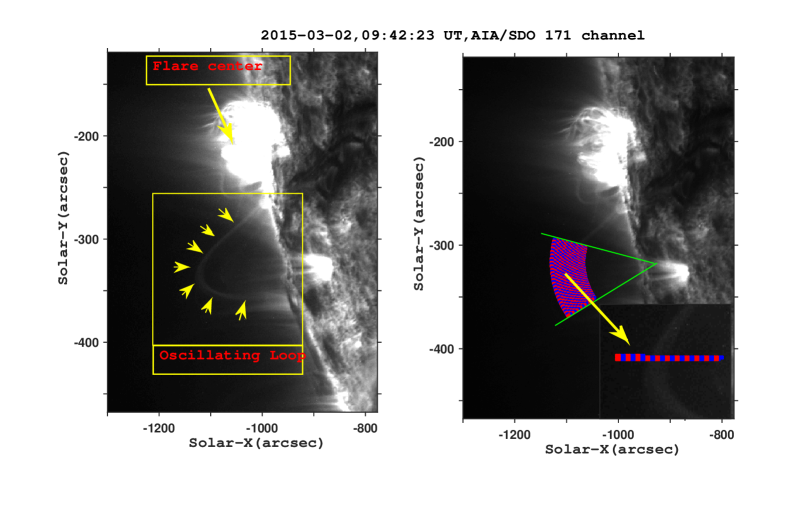
Figure 1.: A snapshot of the flare and near-by loop, like a semi circle, observed by AIA/SDO in 171$\rm{\AA}$ on 2015 March 2, 09:42:23 UT. The locations of the flare and loop are shown with yellow arrows in the left panel. To obtain the transversal coronal loop oscillations, the part of area between two circular arcs containing the loop is subdivided into 30 sectorials that are perpendicular to the visible loop strands. These sectorial areas are then joined by successive cross sections, three pixels wide (see one of these sectorials (zoomed) in the bottom of the right panel).

fig1

The data under analysis here is taken on 2015 March 2, from 09:00:00 UT until 10:30:00 UT and it consists of a series of $1100\times 600$ pixels, sun-centered, subfield images on the 171$\rm{\AA}$ (Fe IX) passband with a time cadence of 12 seconds. The continuous observations of the selected active region loop and its environment monitored with Helioviewer, JHelioviewer, Large Angle and Spectrometric Coronagraph (LASCO) onboard the SoHO, CME catalogue and CACTus CME list show that there is a flare and a LCE in the same parental active region. The solar flare that has been located at position $\rm{(x_{flare},y_{flare})=(-960^{\prime\prime},-192^{\prime\prime})}$ near the loop is started around 2015 March 2, 09:09:00 UT and ended around 2015 March 2, 09:31:12 UT with a peak flux of 1182.3 $\rm{erg/(cm^{2}s)}$ that is occurred at 09:17:12 UT. Also, the LCE that has been located at position $\rm{(x_{LCE},y_{LCE})=(-1006.8^{\prime\prime},-195.6^{\prime\prime})}$ near the loop started around 2015 March 2, 08:21:07 UT and ended around 2015 March 2, 09:01:07 UT. The left panel of Figure fig1 shows a snapshot of the flare and a nearby loop in 171$\rm{\AA}$ on 2015 March 2, 09:24:23 UT that we are analyzing in this paper. The locations of the flare and loop are shown with yellow arrows. To obtain the transversal coronal loop oscillations, the part of area between two circular arcs containing the semi circle-like loop is subdivided many distinct sectorials that are perpendicular to the visible loop strands (Figure fig1, right panel). These sectorial areas are then joined by successive cross sections, three pixels wide. Also, one of the sectorial segments is zoomed in the lower part of the right panel. Figure fig1 shows thirty distinct sectorial areas that are analyzed in detail in the next sections.

3 Data Analysis

Dataa In order to extract the oscillatory nature of transversal coronal loop oscillation, the histogram of images is equalized into histogram of first image by Image Processing Toolbox of Matlab. Histogram equalization is a technique for adjusting image intensities to enhance contrast.

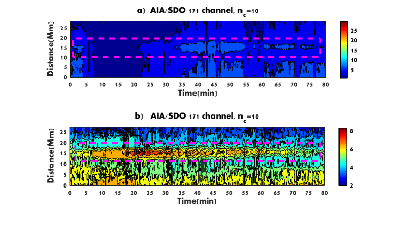
Figure 2.: Typical examples of time$-$distance plot of original intensity (a) for sectorial 10 are shown in the top panel before histogram equalization. Enhanced time$-$distance plot of intensity (b) for sectorial 10 are shown in the bottom panel after histogram equalization. Location of loop enclosed by a red rectangle in the panels.

Fig2

Typical examples of time$-$distance plots of original (a) and histogram equalization (b) intensities time series of images for sectorial 10 are shown in the top and bottom panels of Figure Fig2, respectively. Location of the loop enclosed by a red rectangle in the panels. The part of area between two circular arcs containing the semi circle-like loop is subdivided into 30 sectorial areas that are perpendicular to the visible loop strands. Moreover, each of these sectorial areas are joined by successive cross sections, about three pixels wide. The mean intensity of cross sections as function of time is calculated by dividing the total intensity of cross sections into the number of pixels at each cross sections. A background intensity must be subtracted from the original intensity of cross sections to enhance the contrast of time$-$distance plot and loop axis displacement. Different enhancement algorithms are used to remove the background for an improved visualization of transversal displacements of the loop axis in a time$-$distance plot (see, e.g. Aschwanden and Schrijver 2011; Yuan and Nakariakov  2012; Threlfall et al.  2013; Abedini  2016). Here, following Aschwanden and Schrijver (2011), a running-minimum difference in the form

$$i(n_{c},s_{k},t_{i})=I(n_{c},s_{k},t_{i})-I_{b},$$ (1)

$$I_{b}={\rm{min}}[I(n_{c},s_{k},t_{i-j}),...,I(n_{c},s_{k},t_{i+j})],$$

is used to remove the background intensity of the time$-$distance plots. This running-minimum algorithm subtracts a running-minimum obtained within a time interval with a length of $2j$ from intensity time series of macropixels that are located in the time$-$distance plots of the sectorial areas. Where $n_{c}$ is the number of sectorial areas, $s_{k}$ is the location of the $k$th macropixel at a specific sectorial area, $t_{i}$ is time of ith frame and $t_{i-j},...,t_{i+j}$ represent a time interval of $2j$ frames that symmetrically are placed around $i$th frame in every time slice ($n_{c}=1,k=7,i=2$ corresponds to the seventh macropixel along the sectorial 1 at $t=12s$). The width of selected arcs on the loop are varied between three to six macropixels. An appropriate background is subtracted from the original intensities. Sufficiently enhanced time$-$distance plots of sectorial areas are found by setting the $j=9,...,12$. For example, time$-$distance plots of normalized background-subtracted intensities after histogram equalization ($i_{n}(s_{k},t_{i})=i(s_{k},t_{i})/max[i(s_{1},t_{i}),...,i(s_{end},t_{i})]$) for thirty sectorial areas by running-minimum algorithm are shown in Figures fig3 and fig4. In order to improve visualization of transversal loop oscillation, low oscillation periods ($\rm{P}\leq 36s$) are filtered from intensities after running-minimum subtraction in the thirty time$-$distance plots. The time$-$distance plots of intensities along the sectorial areas show that transversal coronal loop oscillations are occurred in the range of 13 to 43 minutes. Clearly, the enhanced time$-$distance plots of sectorial areas are found by setting the $j=9,...,12$. From Figures fig3 and fig4 it can be seen that the histogram equalization technique has enhanced the contrast of transverse displacements of loop compared to the previous studies (see, e.g. Aschwanden and Schrijver 2011; Goddard et al. 2016). Moreover, in these figures damping and the start times of transverse displacements are clearly visible.

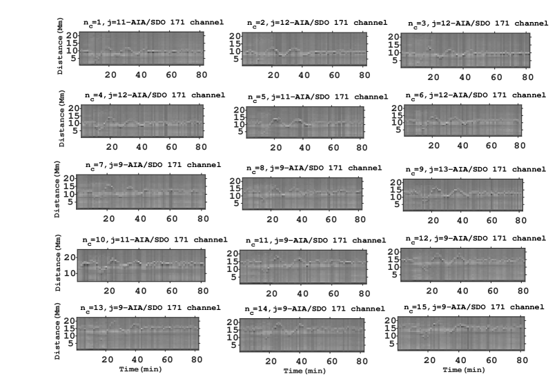
Figure 3.: Running-minimum algorithm to visualize the transversal coronal loop oscillations in time$-$distance plots of intensities ($i_{n}(s_{k},t_{i})=i(s_{k},t_{i})/max[i(s_{1},t_{i}),...,i(s_{end},t_{i})]$) in 171$\AA$ channel of AIA for the sectorial areas 1-15 (time range is 2015 March 2, 9:00:00-10:30:00 UT). In order to improve visualization of transverse displacements of loop low oscillation periods ($\rm{P}\leq 36~{}s$) are filtered from intensities after running-minimum subtraction in the time$-$distance plots. Clearly, transversal coronal loop oscillations is occurred in the panels in the range of 15 to 45 minutes. The number of sectorial area ($n_{c}$) and magnitude value of $j$ are shown on top of each panel.

fig3

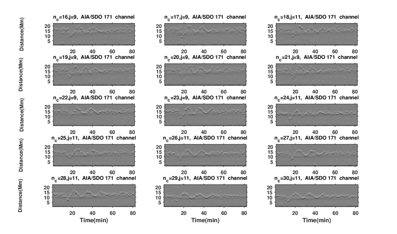
Figure 4.: The same as in Figure 3 but for sectorial areas 16-30.

fig4

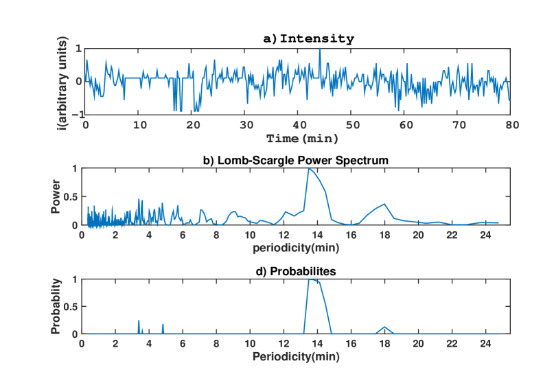
Figure 5.: a) Temporal variation of histogram-equalized and background-subtracted intensity time series of macropixel (13,10) are shown as function of time. b) Lomb-Scargle power spectral density of time series intensity is shown as function of oscillation periods. c) The true-alarm probability of peaks in the Lomb-Scargle power spectra are shown as function of oscillation periods.

fig5

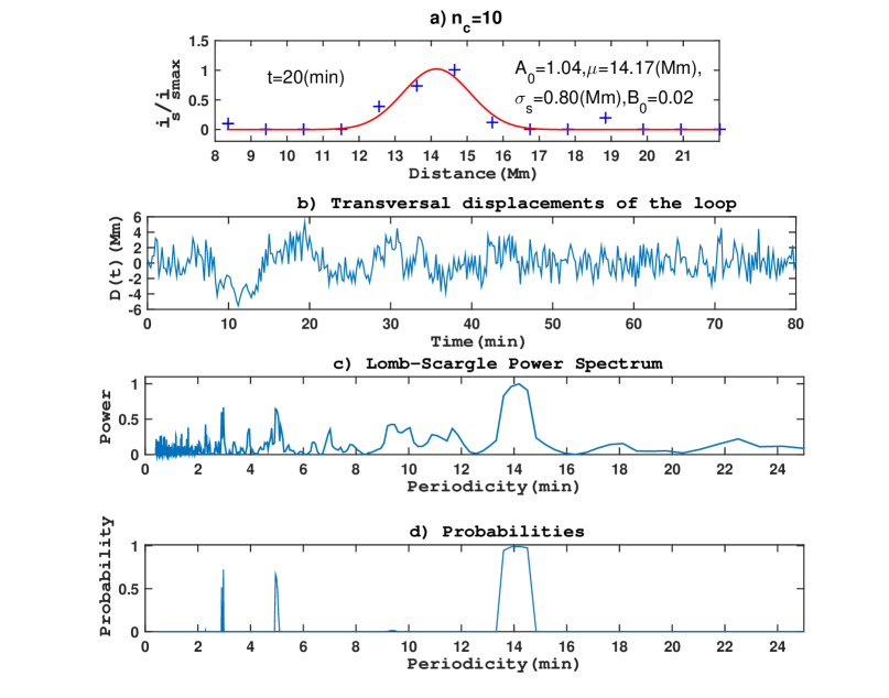
Figure 6.: a) Histogram-equalized, background-subtracted and normalized intensity profile after running-minimum subtraction ($i_{s}(s,t)/i_{smax}(s,t))$ along the sectorial 10 at t=20 min are plotted versus the projected distance. This profile is fitted by an Gaussian function, $G(s,t)=A_{0}(t)\exp(-\frac{(s-\mu(t))^{2}}{2\sigma_{s}(t)^{2}})+B_{0}(t)$ (red line), and fit parameters are shown on the top part of the panel. b) Transversal displacements of the loop axis $D(t)=(\mu(t)-<\mu(t)>$) for sectorial 10 are shown as function of oscillation periods. c) Lomb-Scargle power spectral density of $D(t)$ is shown as function of oscillation periods. d) The true-alarm probability of peaks in the Lomb-Scargle power spectra are shown as function of oscillation periods.

fig6

4 Estimation of the physical parameters of transversal coronal loop oscillation

A coronal loop can be oscillated in various directions. A basic type of coronal loop oscillation is called transverse oscillation. The transverse oscillation can be caused by sausage and kink type modes or it can be caused by the wake of a traveling disturbance from nearby flares. Here, the physical parameters of transversal coronal loop oscillations that are powerful diagnostic tools for coronal seismology are estimated.

4.1 The measurement of transversal coronal loop oscillation periods

In this subsection, oscillation periods of transversal motion of loop segments are estimated. Transversal displacements of the loop have been interpreted in terms of the transverse standing kink mode or the wake of a traveling disturbance of nearby events, since they trigger transversal displacements in the loop axis. In the Figure fig5, intensity time series, Lomb-Scargle power spectral and probability of power spectral of macropixel (13,10) are displayed in the panels a), b) and c), respectively. Intensities of macropixels may be varied by the transversal and/or the longitudinal oscillations. So, in order to infer the transversal coronal loop oscillations as function of time in each time$-$distance plots, a Gaussian function of the form

temp $$G(s,t)=A_{0}(t)\exp[-\frac{(s-\mu(t))^{2}}{2\sigma_{s}(t)^{2}}]+B_{0}(t),$$ (2)

is fitted to the histogram-equalized, background-subtracted and normalized intensities along the paths by Matlab Statistics Toolbox Curve Fitting and Distribution Fitting. This fitting yields the peak of intensity profile $A_{0}(t)$, location of the loop axis $\mu(t)$, standard deviation $\sigma_{s}(t)$, and mean background intensity $B_{0}(t)$ along a specific path in each time, respectively. The oscillation periods of loop axis are calculated by Lomb-Scargle power spectral densities of $D(t)=(\mu(t)-<\mu(t)>$) time series. For example, histogram-equalized, background-subtracted and normalized intensity profile relative to the peak of intensity profile ($i_{s}(s,t)/i_{smax}(s,t)$) for sectorial 10 at $t=20$ minutes are plotted versus the projected distance in the panel a) of Figure fig6. The normalized intensity profiles (blue plus signs) is fitted by an Gaussian function (red line), and fit parameters are displayed in the top part of the panel. Transversal displacements of the loop axis ($D(t)$) for sectorial 10 are shown as function of oscillation periods in the panel b) of Figure fig6. There are a number of techniques that allow to estimate the statistical significance of the detected periodicity, for example the well-known Lomb-Scargle method. This periodgram algorithm gives a better detection accuracy and efficiency for analysis of noisy time series data. Also, the probability of peaks in the power spectral density of noisy time series data happening by chance can be calculated. Furthermore, this algorithm avoids possible incorrect results that may occur from replacement of missing time series data by interpolation methods. For example, the Lomb-Scargle power spectral densities of transversal displacements for sectorial 10 are shown as function of oscillation periods in the panel c) of Figure fig6. Lomb-Scargle power spectral densities of transversal displacements show that there are indeed several statistically dominant peaks of power spectra in the range of P = $2-20$ minutes. The true-alarm probability of significant peaks of power spectra in the panel d) show that only $\rm{P}\approx 3,5$ and 14 minutes are significant oscillation period. Comparisons of probability of peaks before (panel c) of Figure fig5) and after running-minimum subtraction (panel d) of Figure fig6) reveal that significant peaks are quite similar. Furthermore, probability of significant peaks in 30 different sectorial areas reveal three or four significant oscillation periods. One dominant peak around $\rm{P}=14$ minutes is present in all Lomb-Scargle power spectral densities of sectorial areas. But, other peaks are completely different in the power spectral densities.

4.2 The measurement of the damping of transversal loop oscillation

Here, damping times of transversal loop oscillation are measured. Also, the dependence of damping times on amplitude and also on its periodicity are investigated. Lomb-Scargle power spectral densities of $D(t)$ show that spectral components of the transversal displacement along the thirty different sectorial areas are significant at some specified oscillation periods in the range of P = $2-20$ minutes. But, oscillation periods around the $\rm{P}=14$ minutes are almost dominant in all power spectra. Accordingly, the damping time of loop oscillation along the 30 different segments of coronal loop are measured only for common dominant oscillation periods. So, in the Lomb-Scargle power spectral density dominant components of loop axis displacement at each sectorial areas are selected by multiplying each of the components into the Gaussian filter of

temp $$a^{{}^{\prime}}_{j}=\sum_{i=1}^{N_{f}}a_{i}\exp[-\frac{(\nu_{i}-\nu_{j})^{2}}{2\sigma_{\nu}^{2}}],$$ (3)

where the indices $i$ and $j$ are the rank of the harmonics, $N_{f}$ is the total number of the spectral components, $\sigma_{\nu}$ is standard deviation, $\nu_{i}$ and $\nu_{j}$ are the frequency of the $i$th and $j$th harmonics, $a_{i}$ and $a^{{}^{\prime}}_{j}$ are the $i$th and $j$th Fourier coefficient before and after transformation, respectively. Two different kinds of theoretical damping mechanisms have been proposed for transversal coronal loop oscillation: (1) The damping of transversal coronal loop oscillations may be produced by the dissipation mechanism. Generally, resonant absorption is found to be the dominant damping mechanism compared to the other dissipation mechanism (see, e.g. Aschwanden et al. 2003). (2) The damping may be produced by the wake of the traveling disturbance (see, e.g. Rae and Roberts  1982; Uralov  2003; Terradas, Oliver, and Ballester 2005). A localized disturbance from a solar flare propagates toward the loop. As a consequence, coronal loop axis oscillates transversally at the external cutoff frequency, and it is damped approximately with time as $t^{-1/2}$ by the wake of the traveling disturbance. To investigate the damping nature of transversal coronal loop oscillation, the variation of filtered displacement ($D(t)$) with time are fitted by two different forms of damped sine function, $\rm{f_{1}(t)=a_{1}\exp(-(t-t_{0})/\tau_{d})\sin(2\pi(t-t_{0})/P_{1}-\phi_{10})}$ and $\rm{f_{2}(t)=a_{2}(t-t_{0})^{-\alpha}\sin(2\pi(t-t_{0})/P_{2}-\phi_{02})}$.

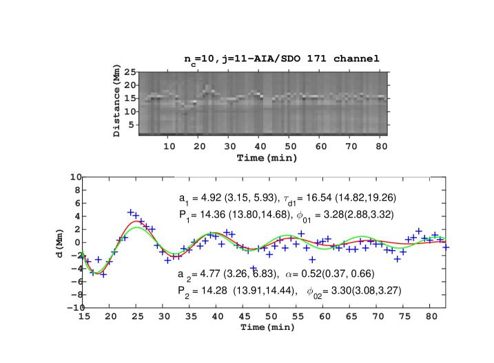
Figure 7.: Template time$-$distance plot for sectorial 10 is shown in the top panel. The variation of filtered transversal displacement ($D(t)$) with time for sectorial 10 at a dominant oscillation period $\rm{P}=14$ min is shown as function of time in the bottom panel. Also, amplitudes are fitted by two different forms of damped sine function, $\rm{f_{1}(t)=a_{1}\exp(-(t-t_{0})/\tau_{d})\sin(2\pi(t-t_{0})/P_{1}-\phi_{01})}$ (red line), $\rm{f_{2}(t)=a_{2}(t-t_{0})^{-\alpha}\sin(2\pi(t-t_{0})/P_{2}-\phi_{02})}$ (green line), and fit parameters are shown on the top and bottom parts of panel, respectively.

fig7

For example, time$-$distance plot for sectorial 10 is displayed in the top panel of Figure fig7. Also, the extracted amplitudes (blue plus signs) at a dominant oscillation period ($\rm{P}=14$ min) are fitted by two different forms of damped sine functions and fit parameters are written in the top and bottom part of panel of Figure fig7, respectively.

Table 1.: Intensity profiles along 30 different sectorial areas of the coronal loop for 400 images are fitted with two different forms of damped sine function, $\rm{f_{1}(t)=a_{1}\exp(-(t-t_{0})/\tau_{d})\sin(2\pi(t-t_{0})/P_{1}-\phi_{10})}$ and $\rm{f_{2}(t)=a_{2}(t-t_{0})^{-\alpha}\sin(2\pi(t-t_{0})/P_{2}-\phi_{02})}$. Magnitudes of fit parameters, such as periodicity, damping time ($\rm{\tau_{d}}$), damping quality ($\rm{\tau_{d}/P}$), magnitude values of $\alpha$ and phase angle ($\phi$) of 30 sectorial areas that they are perpendicular to the visible loop strands observed in the AIA/SDO 171 Å passband.

$\rm{n_{c}}$	$\rm{a_{1}}$	$\rm{\tau_{d1}}$	$\rm{P_{1}}$	$\rm{\tau_{d1}/P_{1}}$	$\rm{\phi_{01}}$	$\rm{a_{2}}$	$\rm{\alpha}$	$\rm{P_{2}}$	$\rm{\phi_{02}}$
	$\rm{(Mm)}$	$\rm{(min)}$	$\rm{(min)}$		$\rm{(rad)}$	$\rm{(Mm)}$		$\rm{(min)}$	$\rm{(rad)}$
1	3.06	18.40	13.86	1.33	3.05	3.23	0.55	13.26	3.04
2	3.98	16.99	14.59	1.17	3.19	4.40	0.69	14.45	3.14
3	3.86	20.06	13.02	1.54	3.04	4.25	0.59	13.31	3.10
4	3.42	21.46	14.68	1.460	3.32	4.45	0.67	14.05	3.24
5	3.35	18.58	15.15	1.22	3.26	4.40	0.65	15.13	3.17
6	4.46	16.67	14.32	1.16	3.22	5.44	0.75	14.16	3.18
7	4.64	19.65	13.16	1.49	3.07	5.01	0.62	13.25	3.14
8	5.10	18.09	13.85	1.31	3.09	5.17	0.59	14.27	3.13
9	5.11	14.94	14.43	1.03	3.21	5.14	0.64	15.03	3.14
10	4.92	16.54	14.36	1.15	3.29	4.77	0.52	14.28	3.30
11	6.24	13.52	14.36	0.91	3.13	7.58	0.75	14.67	3.14
12	6.32	12.16	14.14	0.86	3.05	7.44	0.72	15.02	3.12
13	6.76	15.58	14.58	1.07	3.09	6.70	0.60	14.27	3.14
14	6.36	14.63	15.20	0.96	3.01	6.57	0.62	15.43	3.12
15	5.65	18.65	15.73	1.18	3.19	6.90	0.64	15.75	3.16
16	6.98	15.70	15.20	1.03	3.29	6.45	0.63	14.49	3.14
17	6.60	16.26	14.33	1.13	3.23	6.17	0.65	12.99	3.14
18	-	-	-	-	-	-	-	-	-
19	-	-	-	-	-	-	-	-	-
20	5.64	16.97	12.29	1.38	3.18	6.18	0.58	12.81	3.15
21	5.73	12.34	12.38	0.99	3.12	5.32	0.66	12.25	3.14
22	5.73	15.48	13.97	1.11	3.29	6.25	0.70	13.93	3.24
23	6.17	11.76	12.25	0.87	3.16	6.24	0.67	12.12	3.14
24	6.80	15.00	12.56	1.17	3.22	5.90	0.62	12.39	3.13
25	6.13	17.63	15.80	1.16	3.33	5.51	0.64	15.13	3.14
26	6.16	16.30	13.92	1.17	3.06	5.74	0.65	14.99	3.14
27	6.66	13.40	13.65	0.98	3.14	5.55	0.61	14.13	3.14
28	4.23	16.39	13.91	1.18	3.26	3.20	0.51	13.16	3.14
29	4.44	20.12	14.51	1.39	3.23	4.26	0.61	14.20	3.14
30	4.64	20.29	13.91	1.46	3.28	3.80	0.63	14.32	3.14

results2

The extracted physical quantities such as period of oscillation ($\rm{P}$), damping time ($\rm{\tau_{d}}$), damping quality ($\rm{\tau_{d}/P}$), phase angle ($\phi$) and magnitude values of $\alpha$, for filtered background-subtracted intensity at a sequence of 400 images with a time cadence of 12 seconds are listed in Table results2 for 30 different segments of the coronal loop. The results of this analysis reveal that the magnitude of damping time and damping quality for dominant oscillation periods of segments ($\rm{P}=12.25-15.80$ ) along the coronal loop are within the range of $\rm{\tau_{d}}\simeq 11.76-21.46~{}~{}\rm{min}$. Oscillation of loop segments attenuates with time roughly as $t^{-\alpha}$ that the magnitude of $\alpha$ change from 0.55 to 0.75. The damping quality of loop segments are in the range of $\rm{\tau_{d}/P}\simeq 0.86-1.49$ which clearly indicates that the damping regime is strong for oscillations. Also, these results show that damping times increase with increasing oscillation period. Damping properties decrease slowly with increasing amplitude, but they are not sensitive to the oscillation periods. This range of oscillation periods and damping times of loop segments are in good agreement with previous findings (see, e.g. Nakariakov et al.  1999; Aschwanden et al.  2002; Verwichte et al. 2004; Wang and Solanki  2004)

4.3 The measurement of speed of the flare-generated disturbance and the lower coronal eruption/ejection

Association of transversal coronal loop oscillations with a hypothetical driver of loop oscillations such as a flare, an LCE or a CMEs must be investigated in order to identify a relationship between the excitation and damping of transversal coronal loop oscillations with these phenomena. For this purpose, the possible solar flare, LCE, or CME associated with the oscillating loop were checked using Helioviewer, JHelioviewer, XRS/GOES, LASCO/SoHO, CME catalogue and CACTus CME list. By using these tools, a flare was found near the selected loop at position $\rm{(x_{flare},y_{flare})=(-960^{\prime\prime},-192^{\prime\prime})}.$ It started around 2015 March 2, 09:09:00 UT and ended around 2015 March 2, 09:31:12 UT with a peak flux of 1182.3 $\rm{erg/(cm^{2}s)}$ at 09:17:12 UT. Also, an LCE was detected near the limb at position $\rm{(x_{LCE},y_{LCE})=(-1006.8^{\prime\prime},-195.6^{\prime\prime})}.$ This LCE started around 2015 March 2, 08:21:07 UT and ended around 2015 March 2, 09:01:07 UT. Moreover, in the vicinity of the loop, flare and LCE, CME was not detected one hour before and after of these events start times. Only one CME was found near the oscillating loop with LASCO/SoHO. It started around 2015 March 2, 12:09:05 UT having a radial velocity 269 $\rm{km~{}s^{-1}}$, an angular width 20 degree and a position angle 118 degree, respectively. So, the speeds required for a hypothetical driver of transversal loop oscillations to reach the oscillation loop segments sites from the starting point were estimated. Following Zimovets and Nakariakov (2015), these travel speeds were found in the range of $\rm{v_{flare}=195-520\rm{km~{}s^{-1}}}$ and $\rm{v_{LCE}=14-35\rm{km~{}s^{-1}}}$ by the ratio of the distances between the oscillating loop segments and sites of these events to the time differences between the starting times of LCE and flare with the oscillation loop segments. This result shows that oscillation in a coronal loop cannot be excited by a low-speed shock wave of flare, since the values of the Alfvén speed are mostly more than $800~{}\rm{kms^{-1}}$ (see, e.g. Nakariakov and Ofman 2001; Stepanov et al. 2012; De Moortel and Nakariakov 2012; Zimovets and Nakariakov 2015).

5 Theoretical considerations

Recently, space-based telescope observations have shown that transversal coronal loop oscillations are strongly damped, with damping times of only 1-2 oscillation periods. Theoretically, two different kinds of physical mechanisms have been offered for damping of transversal coronal loop oscillations: damping by dissipation mechanism, and damping by the wake of a traveling disturbance.

5.1 Dissipation mechanism

Several dissipation mechanisms have been proposed for damping of transversal coronal loop oscillations. Theoretical studies investigating the decay of transverse oscillations of coronal loops have concentrated on the effects of phase mixing, resonant absorption, lateral and foot point wave leakage, gravitational stratification and magnetic field divergence. Generally, resonant absorption is found to be the relevant dispassion mechanism for decay of kink mode oscillations (see, e.g. Aschwanden et al.  2003 and references therein). The damping quality of a kink mode oscillating loop with a thin boundary layer due to resonant absorption is given by (see,e.g. Goossens et al.  2002; Ruderman and Roberts  2002; Van Doorsselaere et al. 2004)

$${{\tau_{d}}/\rm{P}=C(\frac{r_{loop}}{l_{skin}})(\frac{1+\frac{\rho_{e}}{\rho_{i}}}{1-\frac{\rho_{e}}{\rho_{i}}})},$$ (4)

where $\rm{C}$ is a constant that depends on the radial density profile, $\rm{r_{loop}}$ is the loop radius, $\rm{l_{skin}}$ is the skin depth of the coronal loop, $\rm{P}$ is the mode period ${2L/(2n-1)C_{K}}$, $n$ is harmonic number of the $n$th harmonic, $\rm{\rho_{i}}$ and $\rm{\rho_{e}}$ are the internal and external plasma density of corona loop, respectively.

5.2 Wake of the traveling disturbance

Uralov (2003) and Terradas et al. (2005) studied the effect of a localized disturbance from a solar flare on transverse motion of a loop. In the zero-$\beta$ plasma limit, they found that dynamics of coronal loop and its environment is governed by the Klein-Gordon equation with cutoff frequency $\omega_{c}=2\pi c_{A}/2L$ by assuming that loop and its environment with a uniform magnetic field is extended between $z=\pm L/2$. These authors pointed out that transversal displacement of coronal loop decays approximately with time as $t^{-1/2}$ by the wake of a traveling disturbance. The wakefield model does not take into account the field-aligned structuring of the corona, in other words, it does not have loops. But, the structuring could affect the wave behaviour quite significantly, as it was shown by Yuan et al. (2015). Decay of transversal loop oscillations due to the wake of a disturbance is not related to any dissipation mechanism such as resonant absorption, phase mixing, etc. Also, these transversal displacement of coronal loops are not necessarily related to the kink mode oscillations, although standing kink oscillations can occur after the decay process by means of the wave packet energy.

6 Discussion and Conclusions

In this paper, it is attempted to provide more insight into the excitation, damping and temporal evolution of transversal displacements of the loop axis near flares, and also an attempt is made to deduce a quantitative relation between oscillation period, damping time, damping quality, oscillation amplitude, dissipation mechanism, lower coronal eruption of some unstable coronal magnetic field configuration and the wake phenomena that is produced by a traveling disturbance in solar coronal loops. For this purpose, the nature of transversal oscillation of a coronal loop ( as observed with AIA/SDO) is analyzed by the histogram-equalization method and Lomb-Scargle periodgram algorithm method that reveal a clearly better detection accuracy and efficiency for analysis of noisy time series data. The values of physical parameters of transversal corona loop segments are extracted in the 171 $\rm{\AA}$ passband. Observational results obtained can be summarized in the following main points:

$\bullet$

The observational results of this study show that histogram equalization technique has enhanced the contrast of transversal coronal loop oscillations in the time$-$distance plots (s ee Figures fig3 and fig4) compared to the previous studies (see, e.g. Aschwanden and Schrijver 2011; Goddard et al. 2016).

$\bullet$

The values of the physical parameters of transversal displacements of the loop segments that have been estimated in this analysis are in good agreement with previous findings (see, e.g. Nakariakov et al.  1999; Aschwanden and Schrijver  2002; Aschwanden et al. 2002; Verwichte et al. 2004; Wang and Solanki  2004; Goddard and Nakariakov 2016).

$\bullet$

The Lomb-Scargle algorithm shows that spectral components of the transversal displacement along the 30 different sectorial areas measured are dominant at some specified oscillation period in the range of P =$2-20$ minutes. But, probability of the observed peaks in the power spectral densities reveal that oscillation periods around the $\rm{P}=14$ minutes are the most dominant component in all power spectral densities of segments.

$\bullet$

The magnitude of damping times and damping qualities of the dominant oscillation period of loop segments ($\rm{P=12.25-15.80}$ minutes) that were determined for the exponential damping are measured in the range of $\rm{\tau_{d}=11.76-21.46}$ minutes and $\rm{\tau_{d}/P=0.86-1.49},$ respectively.

$\bullet$

The magnitude of damping qualities clearly indicate that damping regime is strong for oscillations. Also, the observational results of this analysis reveal that damping qualities decrease slowly with increasing amplitude of the oscillation, but they are not sensitive to the oscillation periods.

$\bullet$

Oscillation of loop segments attenuate with time roughly as that $t^{-\alpha}$ values of $\alpha$ for 30 different segments change from 0.51 to 0.76. These values are in good agreement with theoretical predictions. But, the estimated probability of peaks in Lomb-Scargle power spectral densities of oscillation segments reveal that there is indeed only one dominant peak in each power spectral density. So, considering that the damping of transversal coronal loop oscillation is induced by the wake of a traveling disturbance is not physically compatible with the dissipation mechanism.

$\bullet$

Finally, considering that decaying kink oscillations are excited by a lower coronal eruption of some unstable configuration of coronal magnetised plasma is acceptable as it is compatible with a blast shock wave due to a nearby flare.

Acknowledgments

The author thanks the anonymous referee for the very helpful comments and suggestions. This work was carried out with the support of the University of Qom.
Disclosure of Potential Conflicts of Interest The authors declare that they have no conflicts of interest.

References

- Abedini (2016) Abedini, A.: 2016, Ap&SS 361, 133. DOI. ADS.
- Andries (2009) Andries, J., van Doorsselaere, T., Robedrts, B., Verth, G., Verwichte, E., , R.: 2009, Space Sci. Rev. 149, 3. DOI. ADS.
- Anfinogentov2015 (2015) Anfinogentov, S. A., Nakariakov, V. M., Nisticò, G.: 2015, A&A 583, A136. DOI. ADS.
- Asai (2001) Asai, A., Shimojo, M., Isobe, H., Morimoto, T., Yokoyama, T., Shibasaki, K., Nakajima, H.: 2001, ApJ 562, L103. DOI. ADS.
- Aschwanden (1999) Aschwanden, M. J., Fletcher, L., Schrijver, C. j., Alexander, D .: 1999, ApJ 520, 880. DOI. ADS.
- Aschwanden (2002) Aschwanden, M. J., De Pontieu, B., Schrijver, C. J., Title, A. M.: 2002, Sol. Phys. 206, 99. DOI. ADS.
- Aschwanden (2003) Aschwanden, M. J., Nightingale, R. W., Andries, J., Goossens, M., Van Doorsselaere, T.: 2003, ApJ 598, 1375. DOI. ADS.
- Aschwanden (2004) Aschwanden, M. J.: 2004, Physics of the Solar Corona-An Introduction (New York: Springer) 892. ADS.
- Aschwanden (2004) Aschwanden, M. J., Nakariakov, V. M., Melnikov, V. F.: 2004, ApJ 600, 458. DOI. ADS.
- Aschwanden (2006) Aschwanden, M. J.: 2006, Phil. Trans. R. Soc. 364, 417. DOI. ADS.
- Aschwanden (2011) Aschwanden, M. J. Schrijver, C. J.: 2011, ApJ 736, 102. DOI. ADS.
- Cally (1986) Cally, P. S.: 1986, Sol. Phys. 103, 277. DOI. ADS.
- Cally (2003) Cally, P. S.: 2003, Sol. Phys. 217, 95. DOI. ADS.
- De Moortel (2012) De Moortel, I., Nakariakov, V. M.: 2012, Roy. Soc. London Philos. Trans. Ser. A, 370, 3193. DOI. ADS.
- Ebrahimi (2016) Ebrahimi, Z., Karami, K.: 2016, MNRAS 462, 1002. DOI. ADS.
- Edwin (1982) Edwin, P. M., Roberts, B.: 1982, Sol. Phys. 76, 239. DOI. ADS.
- Edwin (1983) Edwin, P. M., Roberts, B.: 1983, Sol. Phys. 88, 179. DOI. ADS.
- Erdelyi (2003) , R., Petrovay, K., Roberts, B., Aschwanden, M. J.: 2003, Turbulence, Waves and Instabilities in the Solar Plasma (NATO Series II; Dordrecht: Kluwer) ADS.
- Goossens (2002) Goossens, M., Andries, J., Aschwanden, M. J.: 2002, A&A 394, L39. DOI. ADS.
- Goddard (2016) Goddard, C. R., Nisticò, G,. Nakariakov, V. M., Zimovets, I. V.: 2016, A&A 585, L137. DOI. ADS.
- Goddardn (2016) Goddard, C. R., Nakariakov, V. M.: 2016, A&A 590, L5. DOI. ADS.
- Hindman (2014) Hindman, B. W., Jain, R.: 2014, ApJ 784, 103. DOI. ADS.
- Hudson (2004) Hudson, H. S., Warmuth, A.: 2004, ApJ 614, L85. DOI. ADS.
- Kohutova (2016) Kohutova, P., Verwichte, E.: 2016, ApJ 827, L39. DOI. ADS.
- Melnikov (2005) Melnikov, V. F., Reznikova, V. E., Shibasaki, K., Nakariakov, V. M.: 2005, A&A 439, 727. DOI. ADS.
- Morton (2011) Morton, R. J., , R., Jess, D. B., Mathioudakis, M.: 2011, ApJ 729, L18. DOI. ADS.
- Murawski (1993a) Murawski, K., Roberts, B.: 1993a, Sol. Phys. 143, 89. DOI. ADS.
- Murawski (1993b) Murawski, K., Roberts, B.: 1993b, Sol. Phys. 144, 101. DOI. ADS.
- Murawski (1993c) Murawski, K., Roberts, B .:1993c, Sol. Phys. 144, 255. DOI. ADS.
- Nakariakov (1999) Nakariakov, V. M., Ofman, L., DeLuca, E. E., Roberts, B., Davila, J. M.: 1999, Science. 285, 862. DOI. ADS.
- Nakariakov (2001) Nakariakov, V. M., Ofman, L.: 2001, A&A 372, L53. DOI. ADS.
- Nakariakov (2005) Nakariakov, V. M., Verwichte, E.: 2005, Living Rev. Sol. Phys. 2, 3. DOI. ADS.
- Nistico (2013) Nisticò, G., Nakariakov, V. M., Verwichte, E.: 2013, A&A 552, A57. DOI. ADS.
- Pascoe (2016) Pascoe, D. J., Goddard, C. R., Nisticò, G., Anfinogentov, S., Nakariakov, V. M.: 2016, A&A 558, L6. DOI. ADS.
- Rae (1982) Rae, I.C., Roberts, B.: 1982, ApJ 256, 761. DOI. ADS.
- Roberts (1984) Roberts, B., Edwin, P. M., Benz, A. O.: 1984, ApJ 279, 857. DOI. ADS.
- Roberts (2004) oberts, B .: 2004, MHD Waves in the Solar Atmosphere, ed. H. Lacoste (ESA SP-547; Noordwijk: ESA, ESTEC), 1. ADS,
- Ruderman (2002) Ruderman, M.S., Roberts, B.: 2002, ApJ 577, 475. DOI. ADS.
- Ruderman (2009) Ruderman, M. S., , R.: 2009, Space Sci. Rev. 149, 199. DOI. ADS.
- Safari (2007) Safari, H., Nasiri, S., Sobouti, Y.: 2007, A&A 470, 1111. DOI. ADS.
- Schrijver (2002) Schrijver, C. J., Brown, D. S.: 2000, ApJ 537, L69. DOI. ADS.
- Spruit (1982) Spruit, H. C.: 1982, Sol. Phys. 75, 3. DOI. ADS.
- Stepanov (2012) Stepanov, A. V., Zaitsev, V. V., Nakariakov, V. M.: 2012, Coronal Seismology. Physics Uspekhi. 55, A4. DOI. ADS.
- Taroyan (2009) Taroyan, Y., , R.: 2009, Space Sci. Rev. 149, 229. DOI. ADS.
- Terradas (2005) Terradas, J., Oliver, R., Ballester, J. L.: 2005, ApJ 618, L149. DOI. ADS.
- Threlfall (2013) Threlfall, J., De Moortel, I., McIntosh, S. W., Bethge, C.: 2013, A&A 556, A124. DOI. ADS.
- Uchida (1968) Uchida, Y.: 1968, Sol. Phys. 4, 30. DOI. ADS.
- Uchida (1970) Uchida, Y.: 1970, PASJ22, 341. ADS.
- Uralov (2003) Uralov, A. M.: 2003, Astron. Lett. 29, 486. DOI. ADS.
- VanDoorsselaere (2004) Van Doorsselaere, T., Andries, J., Poedts, S., Goossens, M.: 2004, ApJ 606, 1223. DOI. ADS.
- Verwichte (2004) Verwichte, E., Nakariakov, V. M., Ofman, L., DeLuca, E. E.: 2004, Sol. Phys. 223, 77. DOI. ADS.
- Verwichte (2013) Verwichte, E., Van Doorsselaere, T., Foullon, C., White, R. S.: 2013, ApJ 767, 16. DOI. ADS.
- Wangs (2004) Wang, T. J., Solanki, S. K.: 2004, A&A 421, L33. DOI. ADS.
- Yuan (2012) Yuan, D., Nakariakov, V. M.: 2012, A&A 543, A9. DOI. ADS.
- Yuan (2015) Yuan, D., Pascoe, D. J., Nakariakov, V. M., Li, B., Keppens, R.: 2015, A&A 799, 221. DOI. ADS.
- Wang (2004) Wang, T. J.: 2004, SOHO 13 Waves, Oscillations and Small-Scale Transients Events in the Solar Atmosphere, ed. H. Lacoste (ESA SP-547; Noordwijk: ESA, ESTEC). ADS.
- Zimovets (2015) Zimovets, I. V., Nakariakov, V. M.: 2015, A&A 577, A4. DOI. ADS.