Constant-roll tachyon inflation and observational constraints

Abstract

For the constant-roll tachyon inflation, we derive the analytical expressions for the scalar and tensor power spectra, the scalar and tensor spectral tilts and the tensor to scalar ratio to the first order of $\epsilon_{1}$ by using the method of Bessel function approximation. The derived $n_{s}$-$r$ results are compared with the observations, we find that only the constant-roll inflation with $\eta_{H}$ being a constant is consistent with the observations and observations constrain the constant-roll inflation to be slow-roll inflation. The tachyon potential is also reconstructed for the constant-roll inflation which is consistent with the observations.

1 Introduction

The temperature and polarization measurements on the cosmic microwave background anisotropy gave the constraints $n_{s}=0.9645\pm 0.0049$ (68% C.L.) and $r_{0.002}<0.10$ (95% C.L.) [1]. If we take the number of $e$-folds before the end of inflation when a pivotal scale such as $k_{*}=0.002$ Mpc^-1 crosses out the horizon, $N=60$, the observational results suggest that $n_{s}=1-2/N$. This attractor behavior can be realized in chaotic inflation with the quadratic potential [2], the T model with the potential $V(\phi)\sim\tanh^{2n}(\phi/\sqrt{6})$ [3], the E model with the potential $V(\phi)\sim\tanh^{2n}(\phi/\sqrt{6})$ [4], the Starobinsky $R+R^{2}$ model [5], Higgs inflation with the nonminimal coupling $\xi\phi^{2}R$ in the strong coupling limit $\xi\gg 1$ [6, 7], and a class of inflationary models with nonminimal coupling to gravity [8, 9, 10]. The attractor behavior also motivates the parametrization of $n_{s}$ and $r$ by $N$ and the reconstruction of the inflationary potential with the parametrization by neglecting higher order corrections [11, 12, 13, 14, 15, 16, 17, 18, 19, 20, 21, 22, 23, 24, 25, 26, 27, 28, 29, 30, 31].

If the potential of the inflaton is very flat, then the inflaton almost stops rolling and the ultra slow-roll inflation is reached [32, 33]. In the ultra slow-roll inflation, a large curvature perturbation at small scales may be generated to seed primordial black holes [34, 35]. More generally, the constant-roll inflation which includes the slow-roll inflation with small rate of roll and the ultra slow-roll inflation was proposed [36, 37]. In constant-roll inflation, there exists exact solutions, the curvature perturbation may evolve on super-horizon scales and the non-Gaussianity consistency relation may be violated, so the constant-roll inflation has richer physics than the slow-roll inflation does. For the constant-roll or ultra slow-roll inflation, the slow-roll condition is violated, the curvature perturbation may not remain to be a constant outside the horizon [38, 39, 36, 37], so the slow-roll results cannot be applied [33, 40, 36, 37, 41]. For more discussion on constant-roll inflation and its reconstruction, please see [42, 43, 44, 45, 46, 47, 48, 49, 50, 51, 52].

Apart from a canonical scalar field to drive inflation, an effective scalar field with nonlinear kinetic term which describes the tachyon condensate in the string theory [53, 54] also drives inflation and gives the almost scale invariant power spectrum [55, 56, 57, 58, 59, 60, 61, 62]. The reconstruction of the tachyon potential with the help of the parametrization of $n_{s}$ and $r$ in terms of $N$ was discussed in [63, 64, 65]. The rolling tachyon on unstable D-branes in bosonic and superstring theories may behave as dark matter at late time [54], so it naturally leads the transition from early time inflation to late time matter domination. Since the current observation is still unable to address the nature of scalar field, it is interesting to study tachyon inflation and its physical implications. In previous studies, tachyon inflation was considered under the slow-roll condition. The slow-roll condition is violated in the constant-roll inflation when the constant rate of roll is not small, the power spectra for both the scalar and tensor perturbations derived under the slow-roll approximation cannot be applied to the constant-roll inflation. In this paper, we discuss the constant-roll tachyon inflation and derive the analytical formulae for the power spectra . We then use the observational data to constrain the constant-roll tachyon inflationary models. The reconstruction of the tachyon potential is also discussed.

The paper is organized as follows. In section 2, we first review the slow-roll tachyon inflation and introduce four different definitions of slow-roll parameters. The scalar and tensor perturbations for constant-roll tachyon inflation are then derived. In section 3, we derive the formulae for the scalar spectral tilt $n_{s}$ and the tensor-to-scalar ratio $r$ for the four constant-roll inflationary models, and use the observational data to constrain the models. The reconstruction of the tachyon potential for the model with constant $\eta_{H}$ is presented in section 4. The conclusions are drawn in section 5.

2 Tachyon inflation

We start with the effective action for the rolling tachyon

$$S_{T}=-\int d^{4}x\sqrt{-g}\,V(T)\sqrt{1+g^{\mu\nu}\partial_{\mu}T\partial_{\nu}T}.$$ (2.1)

The string motivated potential $V(T)$ has a global maximum at $T=T_{0}$ and a minimum $V\rightarrow 0$ as $T\rightarrow\infty$. Applying the Friedmann-Robertson-Walker metric for the homogeneous and isotropic spacetime, we get the background equations of motion

$$H^{2}=\frac{1}{3}\frac{V}{\sqrt{1-\dot{T}^{2}}},$$ (2.2)

$$\frac{\ddot{T}}{1-\dot{T}^{2}}+3H\dot{T}+\frac{V_{,T}}{V}=0.$$ (2.3)

where $V_{,T}=dV/dT$, and we set $M_{pl}=1/\sqrt{8\pi G}=1$. Combining eqs. (2.2) and (2.3), we get

$$\dot{H}=-\frac{3}{2}H^{2}\dot{T}^{2}.$$ (2.4)

From eq. (2.4), we obtain the acceleration

$$\frac{\ddot{a}}{a}=\dot{H}+H^{2}=H^{2}\left(1-\frac{3}{2}\dot{T}^{2}\right).$$ (2.5)

So the occurrence of inflation $\ddot{a}>0$ is equivalent to $\dot{T}^{2}<2/3$.

2.1 Slow-roll inflation

Under the slow-roll approximations,

$$\dot{T}^{2}\ll 1,$$ (2.6)

$$\quad|\ddot{T}|\ll 3H|\dot{T}|,$$ (2.7)

the background equations (2.2) and (2.3) for the tachyon become

$$H^{2}\approx\frac{V}{3},$$ (2.8)

$$3H\dot{T}\approx-V_{,T}/V.$$ (2.9)

2.2 Slow-roll parameters

In this subsection, we introduce several different definitions of the slow-roll parameters. First, we introduce the horizon flow slow-roll parameters [67]

$$\epsilon_{0}=\frac{H_{o}}{H},$$ (2.10)

$$\epsilon_{i+1}=-\frac{d\ln|\epsilon_{i}|}{dN},$$ (2.11)

where $H_{o}$ is an arbitrary constant. For the tachyon field, the first two slow-roll parameters are [61]

$$\epsilon_{1}=-\frac{\dot{H}}{H^{2}}=\frac{3}{2}\dot{T}^{2},$$ (2.12)

$$\epsilon_{2}=-\frac{d\ln\epsilon_{1}}{dN}=2\frac{\ddot{T}}{H\dot{T}}.$$ (2.13)

By using these slow-roll parameters, the slow-roll conditions (2.6) and (2.7) are expressed as $\epsilon_{1}\ll 1$ and $|\epsilon_{2}|\ll 1$, and inflation ends when $\epsilon_{1}=1$. Under the slow-roll approximations, we also get

$$\epsilon_{1}\approx\frac{1}{2}\frac{V^{2}_{,T}}{V^{3}},$$ (2.14)

$$\epsilon_{2}\approx-2\frac{V_{,TT}}{V^{2}}+3\frac{V^{2}_{,T}}{V^{3}}.$$ (2.15)

The remaining number of $e$-folds $N(t)=\ln(a_{f}/a)$ before the end of inflation is

$$N(t)=\int_{t}^{t_{f}}H(t)dt=\pm\sqrt{\frac{3}{2}}\,\int_{T}^{T_{f}}\frac{H}{\sqrt{\epsilon_{1}}}dT\approx\int^{T}_{T_{f}}\frac{V^{2}}{V_{,T}}dT,$$ (2.16)

where the subscript $f$ denotes the end of inflation, and the $\pm$ sign is the same as the sign of $\dot{T}$. The last approximation is only valid under the slow-roll conditions.

Next, we introduce the Hubble flow slow-roll parameters [68]

$$^{n}\beta_{H}=\frac{2}{3H^{2}}\left(\frac{(H_{,T})^{n-1}H^{(n+1)}}{H^{n}}\right)^{1/n},$$ (2.17)

where $H^{(n)}=d^{n}H/dT^{n}$ and extra $1/H^{2}$ factor is added for the tachyon field. In terms of the Hubble flow slow-roll parameters, the two first order slow-roll parameters are

$$\epsilon_{H}=\frac{2}{3H^{2}}\left(\frac{H_{,T}}{H}\right)^{2}=\epsilon_{1},$$ (2.18)

$$\eta_{H}=\frac{2H_{,TT}}{3H^{3}}=2\epsilon_{1}-\frac{1}{2}\epsilon_{2}.$$ (2.19)

In terms of the slow-roll parameter $\eta_{H}$, the slow-roll condition (2.7) becomes $|\eta_{H}|\ll 1$. Under the slow-roll condition,

$$\eta_{H}\approx-\frac{1}{2}\frac{V_{,T}^{2}}{V^{3}}+\frac{V_{,TT}}{V^{2}}.$$ (2.20)

In analogy with the canonical scalar field, we can also use $\ddot{H}$ to define the slow-roll parameter

$$\epsilon_{2H}=-\frac{\ddot{H}}{2H\dot{H}}=\epsilon_{1}-\frac{1}{2}\epsilon_{2}.$$ (2.21)

In terms of the slow-roll parameter $\epsilon_{2H}$, the slow-roll condition (2.7) becomes $|\epsilon_{2H}|\ll 1$. Under the slow-roll condition,

$$\epsilon_{2H}\approx-\frac{V_{,T}^{2}}{V^{3}}+\frac{V_{,TT}}{V^{2}}.$$ (2.22)

Finally, we introduce the slow-roll parameter

$$\epsilon_{2T}=-\frac{\ddot{T}}{H\dot{T}(1-\dot{T}^{2})}=-\frac{\epsilon_{2}}{2(1-2\epsilon_{1}/3)}.$$ (2.23)

In terms of the slow-roll parameter $\epsilon_{2T}$, the slow-roll condition (2.7) becomes $|\epsilon_{2T}|\ll 1$. For a very flat potential with $V_{,T}\approx 0$, we get the ultra slow-roll inflation and $\epsilon_{2T}\approx 3$, so this slow-roll parameter is useful for the discussion of the ultra slow-roll inflation. Note that when slow-roll condition is satisfied, all the slow-roll parameters introduced above are small.

2.3 The scalar perturbation

In the flat gauge $\delta T(x,t)=0$, the gravitational action $\int d^{4}x\sqrt{-g}R$ plus the action (2.1) for the curvature perturbation $\delta g_{ij}=a^{2}(1+2\zeta)\delta_{ij}$ becomes

$$S=-\frac{3}{2}\int d^{4}x\left[a\dot{T}^{2}(\partial_{i}\zeta)^{2}-a^{3}\frac{\dot{T}^{2}}{1-\dot{T}^{2}}\dot{\zeta}^{2}\right].$$ (2.24)

Using the canonically normalized field $v=z\zeta$, the action (2.24) becomes

$$S=\int d^{3}xd\tau\frac{1}{2}\left[v{{}^{\prime 2}}-c_{s}^{2}(\partial_{i}v)^{2}+\frac{z^{\prime\prime}}{z}v^{2}\right],$$ (2.25)

where the prime denotes the derivative with respect to the conformal time $\tau=\int dt/a$, the effective sound speed is $c_{s}^{2}=1-\dot{T}^{2}=1-2\epsilon_{1}/3$ [59], and

$$z=\frac{\sqrt{3}a\dot{T}}{\sqrt{1-\dot{T}^{2}}}.$$ (2.26)

Now we introduce the quantum operator

$$\hat{v}(\tau,\vec{x})=\int\frac{d^{3}k}{(2\pi)^{3}}\left[v_{k}(\tau)\hat{a}_{k}e^{i\vec{k}\cdot\vec{x}}+v_{k}^{*}(\tau)\hat{a}_{k}^{\dagger}e^{-i\vec{k}\cdot\vec{x}}\right],$$ (2.27)

with the creation and annihilation operators satisfying the standard commutation relations

$$\begin{split}\left[\hat{a}_{k},\ \hat{a}_{k^{\prime}}^{\dagger}\right]=(2\pi)^{3}\delta^{3}(\vec{k}-\vec{k^{\prime}}),\\ \left[\hat{a}_{k},\ \hat{a}_{k^{\prime}}\right]=\left[\hat{a}_{k}^{\dagger},\ \hat{a}_{k^{\prime}}^{\dagger}\right]=0,\end{split}$$ (2.28)

By choosing the Bunch-Davies vacuum $\hat{a}_{k}|0\rangle=0$ [69], the mode function $v_{k}$ obeys the normalization condition

$$v_{k}^{\prime}v_{k}^{*}-v_{k}{v_{k}^{*}}^{\prime}=-i.$$ (2.29)

Varying the action (2.25), we obtain the Mukhanov-Sasaki equation for the mode function $v_{k}(\tau)$ [61],

$$v_{k}^{\prime\prime}+\left(c_{s}^{2}k^{2}-\frac{z^{\prime\prime}}{z}\right)v_{k}=0.$$ (2.30)

To solve the Mukhanov-Sasaki equation (2.30), we need the expression for $z^{\prime\prime}/z$. In terms of the slow-roll parameters, from the definition (2.26) we get [61]

$$\dot{z}=Hz\left[1+\frac{\epsilon_{2}}{2\left(1-\frac{2}{3}\epsilon_{1}\right)}\right],$$ (2.31)

$$\frac{\ddot{z}}{z}=-H^{2}\epsilon_{1}\left[1+\frac{\epsilon_{2}}{2\left(1-\frac{2}{3}\epsilon_{1}\right)}\right]+H^{2}\left[1+\frac{\epsilon_{2}}{2\left(1-\frac{2}{3}\epsilon_{1}\right)}\right]^{2}+\frac{H^{2}\epsilon_{2}^{2}\epsilon_{1}}{3\left(1-\frac{2}{3}\epsilon_{1}\right)^{2}}+\frac{H\dot{\epsilon_{2}}}{2\left(1-\frac{2}{3}\epsilon_{1}\right)},$$ (2.32)

$$z^{\prime}=\frac{dz}{d\tau}=a\dot{z}=aHz\left[1+\frac{\epsilon_{2}}{2\left(1-\frac{2}{3}\epsilon_{1}\right)}\right],$$ (2.33)

$$\frac{z^{\prime\prime}}{z}=a^{2}H^{2}\left[1+\frac{\epsilon_{2}}{2\left(1-\frac{2}{3}\epsilon_{1}\right)}\right]+\frac{a^{2}\ddot{z}}{z}.$$ (2.34)

From the relation

$$\frac{d}{d\tau}\left(\frac{1}{aH}\right)=-1+\epsilon_{1},$$ (2.35)

we get

$$\frac{1}{aH}=-\tau+\int\epsilon_{1}d\tau=\tau(\epsilon_{1}-1)-\int\tau\frac{\epsilon_{1}}{d\tau}d\tau,$$ (2.36)

Since

$$\dot{\epsilon_{1}}=H\epsilon_{1}\epsilon_{2},$$ (2.37)

so

$$\int\tau\frac{\epsilon_{1}}{d\tau}d\tau=\int aH\tau\epsilon_{1}\epsilon_{2}d\tau.$$ (2.38)

If $\epsilon_{2}$ is a constant, to the first order of $\epsilon_{1}$, we get

$$\int\tau\frac{\epsilon_{1}}{d\tau}d\tau=-\epsilon_{2}\int\epsilon_{1}d\tau.$$ (2.39)

Combining eqs. (2.36) and (2.39), to the first order of $\epsilon_{1}$, for constant $\epsilon_{2}$ we obtain [41]

$$\frac{1}{aH}\approx\left(\frac{\epsilon_{1}}{1-\epsilon_{2}}-1\right)\tau.$$ (2.40)

Because we derive the above result with the relation (2.37), so the result (2.40) does not apply to the case with $\epsilon_{1}$ being a constant or large. Since we need the relation (2.40), we assume $\epsilon_{2}$ is a constant and $\epsilon_{1}$ is small in this section for the convenience of discussion. Substituting eq. (2.40) into (2.34), we can express $z^{\prime\prime}/z$ in terms of a function of the slow-roll parameters $\epsilon_{1}$ and $\epsilon_{2}$ divided by $\tau^{2}$, and we rewrite eq. (2.30) as

$$v_{k}^{\prime\prime}+\left(c_{s}^{2}k^{2}-\frac{\nu^{2}-1/4}{\tau^{2}}\right)v_{k}=0,$$ (2.41)

where

$$\nu^{2}=\frac{1}{4}+\frac{z^{\prime\prime}}{z}\tau^{2}$$ (2.42)

depends on the slow-roll parameters $\epsilon_{1}$ and $\epsilon_{2}$ only. For the slow-roll inflation, $\epsilon_{1}$ and $\epsilon_{2}$ changes slowly, $\nu$ can be approximated as a constant. For the constant-roll inflation, $\nu$ can also be approximated as a constant. For either case, $\nu$ is almost a constant, the solution to eq. (2.41) for the mode function $v_{k}$ is the Hankel function of order $\nu$. If $\epsilon_{2}$ is too large, then from eq. (2.37), we see that $\dot{\epsilon}_{1}$ may not small, and the Bessel function approximation may break down [41]. Here we don’t consider this issue and leave it for future discussion. By matching the Hankel function to the asymptotic plane wave solution with $k\rightarrow\infty$ which is consistent with the normalization condition (2.29), we get the curvature perturbation on super-horizon scales,

$$|\zeta_{k}|=\frac{|v_{k}|}{z}=2^{\nu-2}\frac{\Gamma(\nu)}{\Gamma(3/2)}\left[\frac{1}{aH}\left(1+\frac{\epsilon_{1}}{1-\epsilon_{2}}\right)\right]^{\frac{1}{2}-\nu}(c_{s}k)^{-\nu}/z.$$ (2.43)

On super-horizon scales, $k\rightarrow 0$, the curvature perturbation $\zeta$ may not remain to be a constant. In this paper, we focus on the usual situation that the curvature perturbation remains constant. Therefore, the power spectrum of the scalar perturbation is

$$P_{\zeta}=\frac{k^{3}}{2\pi^{2}}|\zeta_{k}|^{2}=\left.\frac{2^{2\nu-3}}{2c_{s}\epsilon_{1}}\left[\frac{\Gamma(\nu)}{\Gamma(3/2)}\right]^{2}\left(1+\frac{\epsilon_{1}}{1-\epsilon_{2}}\right)^{1-2\nu}\left(\frac{H}{2\pi}\right)^{2}\left(\frac{c_{s}k}{aH}\right)^{3-2\nu}\right|_{c_{s}k=aH}.$$ (2.44)

The amplitude of the scalar perturbation is

$$A_{s}=\left.\frac{2^{2\nu-3}}{c_{s}}\left[\frac{\Gamma(\nu)}{\Gamma(3/2)}\right]^{2}\left(\frac{1-\epsilon_{2}+\epsilon_{1}}{1-\epsilon_{2}}\right)^{1-2\nu}\frac{H^{2}}{8\pi^{2}\epsilon_{1}}\right|_{c_{s}k=aH}.$$ (2.45)

The scalar spectral tilt is

$$n_{s}-1=\frac{d\ln P_{\zeta}}{d\ln k}=3-2\nu.$$ (2.46)

2.4 The tensor perturbation

For the tensor perturbation $\delta g_{ij}=a^{2}\gamma_{ij}$, to the second order, the gravitational action plus the action (2.1) becomes

$$S=\frac{1}{8}\int d^{4}x\left[a^{3}(\dot{\gamma}_{ij})^{2}-a(\gamma_{ij,k})^{2}\right],$$ (2.47)

where $\gamma_{ij}=\sum_{s=+,\times}e_{ij}^{s}\gamma^{s}$. Following the same procedure as that in the scalar perturbation, we introduce the normalized field $u=a\gamma/\sqrt{2}$, and get eq. (2.41) with $v$ replaced by $u$, and $\nu$ replaced by $\mu$, where

$$\mu^{2}=\frac{1}{4}+\frac{a^{\prime\prime}}{a}\tau^{2},$$ (2.48)

and

$$\frac{a^{\prime\prime}}{a}=a^{2}H^{2}(2-\epsilon_{1}),$$ (2.49)

so the tensor spectrum is

$$P_{T}=2^{2\mu}\left[\frac{\Gamma(\mu)}{\Gamma(3/2)}\right]^{2}\left(1+\frac{\epsilon_{1}}{1-\epsilon_{2}}\right)^{1-2\mu}\left(\frac{H}{2\pi}\right)^{2}\left(\frac{k}{aH}\right)^{3-2\mu}.$$ (2.50)

The tensor spectral tilt is

$$n_{T}=\frac{d\ln P_{T}}{d\ln k}=3-2\mu.$$ (2.51)

Combining eqs. (2.45) and (2.50), to the first order of $\epsilon_{1}$, we get the tensor to scalar ratio

$$r=2^{2(\mu-\nu)+4}\left[\frac{\Gamma(\mu)}{\Gamma(\nu)}\right]^{2}\epsilon_{1}.$$ (2.52)

3 The constant-roll inflationary models

3.1 Constant $\epsilon_{2}$

In this subsection, we consider the case that $\epsilon_{2}$ is a constant and derive the formulae for $n_{s}$ and $r$ to the first order of $\epsilon_{1}$. From eq. (2.40), to the first order of $\epsilon_{1}$, we get

$$aH\approx-\frac{1}{\tau}\left(1+\frac{\epsilon_{1}}{1-\epsilon_{2}}\right).$$ (3.1)

Using $\dot{\epsilon}_{2}=0$ and combining eqs. (2.32), (2.34), (2.42) and (3.1), to the first order of $\epsilon_{1}$, we obtain

$$\nu\approx\frac{1}{2}|3+\epsilon_{2}|+\frac{(4\epsilon_{2}^{3}-4\epsilon_{2}^{2}-27\epsilon_{2}-18)\epsilon_{1}}{6|3+\epsilon_{2}|(\epsilon_{2}-1)},$$ (3.2)

$$\mu\approx\frac{3}{2}+\frac{3+\epsilon_{2}}{3(1-\epsilon_{2})}\epsilon_{1}.$$ (3.3)

Substituting eqs. (3.2) and (3.3) into eqs. (2.46) and (2.52), to the first order of $\epsilon_{1}$, we derive that

$$n_{s}\approx 4-|3+\epsilon_{2}|+\frac{(18-4\epsilon_{2}^{3}+4\epsilon_{2}^{2}+27\epsilon_{2})\epsilon_{1}}{3|3+\epsilon_{2}|(\epsilon_{2}-1)},$$ (3.4)

$$r\approx 2^{3-|3+\epsilon_{2}|}\left(\frac{\Gamma[3/2]}{\Gamma[|3+\epsilon_{2}|/2]}\right)^{2}\,16\epsilon_{1}.$$ (3.5)

If the slow-roll condition is satisfied, $|\epsilon_{2}|\ll 1$, the results become $n_{s}=1-2\epsilon_{1}-\epsilon_{2}$ and $r=16\epsilon_{1}$ [59, 60, 61, 64], so the results for the slow-roll tachyon inflation are recovered. To the first order of $\epsilon_{1}$, the result (3.4) is different from that for the canonical scalar field found in [70].

Since $\epsilon_{2}$ is a constant, from the definition (2.13), we get

$$\epsilon_{1}(N)=C\exp(-\epsilon_{2}N),$$ (3.6)

where $C$ is an integration constant. At the end of inflation, $N=0$, $\epsilon_{1}(N)=1$, so $C=1$. Substituting eq. (3.6) into eqs. (3.4) and (3.5), we can calculate $n_{s}$ and $r$ for the model with constant $\epsilon_{2}$, and the results along with the Planck 2015 constraints [1] are shown in figure 1. In figure 1, we plot the results by varying $\epsilon_{2}$ with $N=50$ and $N=60$, and the black lines denote the results for the model with constant $\epsilon_{2}$. From figure 1, we see that the model is ruled out by observations at the $3\sigma$ C.L.

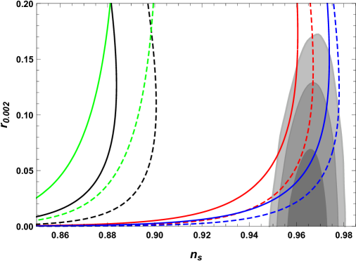
Figure 1: The marginalized 68%, 95% and 99.8% confidence level contours for $n_{s}$ and $r$ from Planck 2015 data [1] and the observational constraints on $n_{s}-r$ for different constant-roll inflationary models. The solid and dashed lines represent $N=50$ and $N=60$, respectively. The green lines denote the model with constant $\epsilon_{2T}$, the black lines denote the model with constant $\epsilon_{2}$, the red lines denote the model with constant $\epsilon_{2H}$, and the blue lines denote the model with constant $\eta_{H}$.

3.2 Constant $\epsilon_{2H}$

In this subsection, we consider the case that $\epsilon_{2H}$ is a constant and derive the formulae for $n_{s}$ and $r$ to the first order of $\epsilon_{1}$. From eq. (2.21), we have

$$\epsilon_{2}=2(\epsilon_{1}-\epsilon_{2H}),$$ (3.7)

$$\dot{\epsilon}_{2}=4H\epsilon_{1}(\epsilon_{1}-\epsilon_{2H}).$$ (3.8)

Replacing $\epsilon_{2}$ with $\epsilon_{2H}$ by the relation (3.7) and using the result (3.8) for $\dot{\epsilon}_{2}$, to the first order of $\epsilon_{1}$, we get

$$aH\approx-\frac{1}{\tau}\left(1+\frac{\epsilon_{1}}{1+2\epsilon_{2H}}\right),$$ (3.9)

$$\nu\approx\frac{1}{2}|3-\epsilon_{2H}|+\frac{(16\epsilon_{2H}^{3}-16\epsilon_{2H}^{2}-21\epsilon_{2H}+18)\epsilon_{1}}{3|3-\epsilon_{2H}|(2\epsilon_{2H}+1)},$$ (3.10)

$$\mu\approx\frac{3}{2}+\frac{3-2\epsilon_{2H}}{3(1+2\epsilon_{2H})}\epsilon_{1}.$$ (3.11)

Substituting eqs. (3.10) and (3.11) into eqs. (2.46) and (2.52), to the first order of $\epsilon_{1}$, we obtain

$$n_{s}\approx 4-|3-2\epsilon_{2H}|+\frac{(-32\epsilon_{2H}^{3}+32\epsilon_{2H}^{2}+42\epsilon_{2H}-36)\epsilon_{1}}{3|3-2\epsilon_{2H}|(2\epsilon_{2H}+1)},$$ (3.12)

$$r\approx 2^{3-|3-2\epsilon_{2H}|}\left(\frac{\Gamma[3/2]}{\Gamma[|3-2\epsilon_{2H}|/2]}\right)^{2}16\epsilon_{1}.$$ (3.13)

In the slow-roll limit, $|\epsilon_{2H}|\ll 1$, we get $n_{s}=1-4\epsilon_{1}+2\epsilon_{2H}$ and $r=16\epsilon_{1}$ which are consistent with slow-roll results.

Since $\epsilon_{2H}$ is a constant, from the definition (2.13) and the condition $\epsilon_{1}(N=0)=1$, we derive that

$$\epsilon_{1}(N)=\frac{\epsilon_{2H}\exp(2\epsilon_{2H}N)}{\exp(2\epsilon_{2H}N)+\epsilon_{2H}-1},$$ (3.14)

Substituting eq. (3.14) into eqs. (3.12) and (3.13), we can calculate $n_{s}$ and $r$ for the model with constant $\epsilon_{2H}$, and the results along with the Planck 2015 constraints [1] are shown in figure 1. In figure 1, we plot the results by varying $\epsilon_{2H}$ with $N=50$ and $N=60$, and the red lines denote the results for the model with constant $\epsilon_{2H}$. From figure 1, we see that the model is inconsistent with the observations at the $1\sigma$ C.L.

3.3 Constant $\eta_{H}$

For the model with constant $\eta_{H}$, from eqs. (2.19) and (2.37) we get

$$\epsilon_{2}=2(2\epsilon_{1}-\eta_{H}),$$ (3.15)

$$\dot{\epsilon}_{2}=8H\epsilon_{1}(2\epsilon_{1}-\eta_{H}).$$ (3.16)

Replacing $\epsilon_{2}$ with $\eta_{H}$ by the relation (3.15) and using the result (3.16) for $\dot{\epsilon}_{2}$, to the first order of $\epsilon_{1}$, we have

$$aH\approx-\frac{1}{\tau}\left(1+\frac{\epsilon_{1}}{1+2\eta_{H}}\right),$$ (3.17)

$$\nu\approx\frac{1}{2}|3-2\eta_{H}|+\frac{(16\eta_{H}^{3}-40\eta_{H}^{2}-15\eta_{H}+27)\epsilon_{1}}{3|3-2\eta_{H}|(2\eta_{H}+1)},$$ (3.18)

$$\mu\approx\frac{3}{2}+\frac{3-2\eta_{H}}{3(1+2\eta_{H})}\epsilon_{1}.$$ (3.19)

Substituting eqs. (3.18) and (3.19) into eqs. (2.46) and (2.52), to the first order of $\epsilon_{1}$, we obtain

$$n_{s}\approx 4-|3-2\eta_{H}|+\frac{(-32\eta_{H}^{3}+80\eta_{H}^{2}+30\eta_{H}-54)\epsilon_{1}}{3|3-2\eta_{H}|(2\eta_{H}+1)},$$ (3.20)

$$r\approx 2^{3-|3-2\eta_{H}|}\left(\frac{\Gamma[3/2]}{\Gamma[|3-2\eta_{H}|/2]}\right)^{2}\,16\epsilon_{1}.$$ (3.21)

In the slow-roll limit, $|\eta_{H}|\ll 1$, we get $n_{s}=1-6\epsilon_{1}+2\eta_{H}$ and $r=16\epsilon_{1}$ which are consistent with the slow-roll results. The slow-roll results are the same as those for the canonical scalar field with $\eta_{V}$.

Since $\eta_{H}$ is a constant, from the definition (2.13) and the condition $\epsilon_{1}(N=0)=1$, we get

$$\epsilon_{1}(N)=\frac{\eta_{H}\exp(2\eta_{H}N)}{2\exp(2\eta_{H}N)+\eta_{H}-2},$$ (3.22)

Plugging eq. (3.22) into eqs. (3.20) and (3.21), we express $n_{s}$ and $r$ in terms of $N$ and $\eta_{H}$. By choosing $N=50$ and $N=60$, and varying the value of $\eta_{H}$, we plot the $n_{s}$-$r$ results for the model with constant $\eta_{H}$ along with the Planck 2015 constraints [1] in figure 1. The blue lines denote the $n_{s}$-$r$ results for the model with constant $\eta_{H}$. From figure 1, we see that the model with constant $\eta_{H}$ is consistent with the observations at $1\sigma$ C.L. For $N=50$, the $1\sigma$ constraint is $-0.0135<\eta_{H}<-0.0036$, the $2\sigma$ constraint is $-0.0184<\eta_{H}<0.006$, and the $3\sigma$ constraint is $-0.0207<\eta_{H}<0.0146$. For $N=60$, the $1\sigma$ constraint is $-0.018<\eta_{H}<-0.006$, the $2\sigma$ constraint is $-0.0212<\eta_{H}<0.0013$, and the $3\sigma$ constraint is $-0.023<\eta_{H}<0.007$. If we take $\eta_{H}=-0.009$ and $N=60$, we get $\epsilon_{1}=0.0023$, $n_{s}=0.968$, $r=0.036$. Since observations require that $\epsilon_{1}$ and $\eta_{H}$ are both small, so the slow-roll condition is satisfied and this constant-roll inflation with constant $\eta_{H}$ is also a slow-roll inflation. If we use the slow-roll formulae to fit the observations, the $1\sigma$ constraint is $-0.014<\eta_{H}<-0.0039$, the $2\sigma$ constraint is $-0.018<\eta_{H}<0.0068$, and the $3\sigma$ constraint is $-0.02<\eta_{H}<0.0168$ for $N=50$. For $N=60$, the $1\sigma$ constraint is $-0.018<\eta_{H}<-0.0067$, the $2\sigma$ constraint is $-0.021<\eta_{H}<0.0015$, and the $3\sigma$ constraint is $-0.023<\eta_{H}<0.01$. The $2\sigma$ and $3\sigma$ upper bounds given by the slow-roll formulae are larger than those given by the constant-roll formulae, so even in the slow-roll regime, the results are not exactly the same, but the constant-roll formulae (3.20) and (3.21) are more accurate.

3.4 Constant $\epsilon_{2T}$

For the model with constant $\epsilon_{2T}$, from eqs. (2.23) and (2.37) we get

$$\epsilon_{2}=-2\epsilon_{2T}\left(1-\frac{2}{3}\epsilon_{1}\right),$$ (3.23)

$$\dot{\epsilon}_{2}=-\frac{8}{3}H\epsilon^{2}_{2T}\epsilon_{1}\left(1-\frac{2}{3}\epsilon_{1}\right).$$ (3.24)

Replacing $\epsilon_{2}$ with $\epsilon_{2T}$ by the relation (3.23) and using the result (3.24) for $\dot{\epsilon}_{2}$, to the first order of $\epsilon_{1}$, we obtain

$$aH\approx-\frac{1}{\tau}\left(1+\frac{\epsilon_{1}}{1+2\epsilon_{2T}}\right),$$ (3.25)

$$\nu\approx\frac{1}{2}|3-2\epsilon_{2T}|+\frac{(4\epsilon_{2T}^{2}-7\epsilon_{2T}+3)\epsilon_{1}}{|3-2\epsilon_{2T}|(2\epsilon_{2T}+1)},$$ (3.26)

$$\mu\approx\frac{3}{2}+\frac{3-2\epsilon_{2T}}{3(1+2\epsilon_{2T})}\epsilon_{1}.$$ (3.27)

Plugging the results (3.26) and (3.27) into eqs. (2.46) and (2.52), we have

$$n_{s}\approx 4-|3-2\epsilon_{2T}|+\frac{2(4\epsilon_{2T}^{2}-7\epsilon_{2T}+3)\epsilon_{1}}{3|3-2\epsilon_{2T}|(2\epsilon_{2T}+1)},$$ (3.28)

$$r\approx 2^{3-|3-2\epsilon_{2T}|}\left(\frac{\Gamma[3/2]}{\Gamma[|3-2\epsilon_{2T}|/2]}\right)^{2}\,16\epsilon_{1}.$$ (3.29)

In the slow-roll limit, we get $|\epsilon_{2T}|\ll 1$, $n_{s}=1+2\epsilon_{1}/3+2\epsilon_{2T}$.

For constant $\epsilon_{2T}$, from the definition (2.13) and the condition $\epsilon_{1}(N=0)=1$, we derive that

$$\epsilon_{1}(N)=\frac{3}{\exp(-2\epsilon_{2T}N)+2}.$$ (3.30)

Substituting eq. (3.30) into eqs. (3.28) and (3.29), we express $n_{s}$ and $r$ in terms of $N$ and $\epsilon_{2T}$. By choosing $N=50$ and $N=60$, and varying the value of $\epsilon_{2T}$, we plot the $n_{s}$-$r$ results for the model with constant $\epsilon_{2T}$ along with the Planck 2015 constraints [1] in figure 1. The green lines denote the results for the model with constant $\epsilon_{2T}$. From figure 1, we see that the model with constant $\epsilon_{2T}$ is excluded by the observations at the $3\sigma$ C.L.

4 The reconstruction of the potential

From the analysis in the previous section, we see that only the model with constant $\eta_{H}$ is consistent with the observations and it is constrained to be a slow-roll inflation. In this section, we follow the procedure presented in [64] for the slow-roll inflation to reconstruct the tachyon potential with constant $\eta_{H}$. Combining eqs. (2.14) and (2.16), we get

$$\epsilon_{1}\approx\frac{V_{,N}}{2V},$$ (4.1)

where $V_{,N}=dV/dN$. Substituting eq. (3.22) into (4.1), we obtain

$$V(N)\approx V_{0}\left|\eta_{H}+2\exp(2\eta_{H}N)-2\right|^{\frac{1}{2}},$$ (4.2)

and

$$A_{s}\approx\frac{V}{24\pi^{2}\epsilon_{1}}=\frac{V_{0}|\eta_{H}+2\exp(2\eta_{H}N)-2|}{24\pi^{2}\epsilon_{1}}.$$ (4.3)

If we take $\eta_{H}=-0.009$, $A_{s}=2.2\times 10^{-9}$ and $N=60$, we get $V_{0}=1.0386\times 10^{-9}$. From the relation

$$dT\approx\pm\frac{\sqrt{V_{,N}}}{V}dN,$$ (4.4)

we get

$$T-T_{0}\approx\sqrt{\frac{2}{|\eta_{H}|V_{0}}}\frac{\exp(\eta_{H}N)}{|\eta_{H}-2|^{3/4}}\,_{2}F_{1}\left(\frac{1}{2},\frac{3}{4};\frac{3}{2};\frac{2\exp(\eta_{H}N)}{2-\eta_{H}}\right).$$ (4.5)

If we take $\eta_{H}=-0.009$, $A_{s}=2.2\times 10^{-9}$ and $N=60$, we find that the field excursion is $\Delta T=T_{*}-T_{f}=1.76\times 10^{5}$ and this result is consistent with the lower bound on the field excursion derived in [64]. Combining eqs. (4.2) and (4.5), we can obtain the potential $V(T)$ and the reconstructed potential for $\eta_{H}=-0.009$ is shown in figure 2. From figure 2, we see that $V(T)$ has a maximum at $T=T_{0}$ and $V(T)\rightarrow 0$ as $T\rightarrow 0$, this property is consistent with that of the string inspired potential. Because it is difficult to obtain an analytical expression for $N$ in terms of $T$ from eq. (4.5) in general, here we give the analytical behavior of $V(T)$ around $T=T_{0}$. As $T\rightarrow T_{0}$, from eq. (4.5), we get

$$e^{2\eta_{H}N}\approx\frac{1}{2}|2-\eta_{H}|^{3/2}|\eta_{H}|V_{0}(T-T_{0})^{2}.$$ (4.6)

Substituting eq. (4.6) into eq. (4.2), we obtain the potential around $T=T_{0}$,

$$V(T)\approx|2-\eta_{H}|^{1/2}V_{0}\left[1-\frac{1}{2}|2-\eta_{H}|^{1/2}|\eta_{H}|V_{0}(T-T_{0})^{2}\right].$$ (4.7)

Figure 2: The reconstructed potential normalized by $V_{0}=1.0386\times 10^{-9}$.

5 Conclusions

We introduce four different definitions for the slow-roll parameters. For these four different constant-roll inflationary models, we derive the analytical expressions for the scalar and tensor power spectra, the scalar and tensor spectral tilts and the tensor to scalar ratio to the first order of $\epsilon_{1}$ by using the method of Bessel function approximation. These results reduce to those for slow-roll inflation if slow-roll conditions are satisfied. We also use the observational data to constrain the constant-roll inflationary models, and we find that the constant-roll inflationary models with constant $\epsilon_{2}$ or constant $\epsilon_{2T}$ are ruled out by the observations at the $3\sigma$ C.L. The model with constant $\epsilon_{2H}$ is inconsistent with the observations at the $1\sigma$ C.L. The model with constant $\eta_{H}$ is consistent with the observations, and the 1$\sigma$ constraint is $-0.0135<\eta_{H}<-0.0036$ if we take $N=50$; the 1$\sigma$ constraint is $-0.018<\eta_{H}<-0.006$ if we take $N=60$. Since the observational constraints tell us that $|\eta_{H}|\ll 1$, so the slow-roll conditions are satisfied and the constant-roll inflation is also a slow-roll inflation. Following the reconstruction procedure for the slow-roll inflation, we reconstruct the tachyon potential for the model with constant $\eta_{H}$. The reconstructed tachyon potential satisfies the property for the string inspired potential, but the possible origin of the potential from string theory needs further study. If we choose $\eta_{H}=-0.009$, $A_{s}=2.2\times 10^{-9}$ and $N=60$, we get $\epsilon_{1}=0.0023$, $n_{s}=0.968$, $r=0.036$, $V_{0}=1.0386\times 10^{-9}$ and $\Delta T=T_{*}-T_{f}=1.76\times 10^{5}$. The field excursion for the tachyon is consistent with the general lower bound. Although $\eta_{H}$ is constrained to be small and slow-roll inflation applies, the results for constant-roll inflation are more general and have broad applications.

References

- [1] Planck collaboration, P. A. R. Ade et al., Planck 2015 results. XX. Constraints on inflation, Astron. Astrophys. 594 (2016) A20, [1502.02114].
- [2] A. D. Linde, Chaotic Inflation, Phys. Lett. B 129 (1983) 177–181.
- [3] R. Kallosh and A. Linde, Universality Class in Conformal Inflation, JCAP 1307 (2013) 002, [1306.5220].
- [4] R. Kallosh and A. Linde, Non-minimal Inflationary Attractors, JCAP 1310 (2013) 033, [1307.7938].
- [5] A. A. Starobinsky, A New Type of Isotropic Cosmological Models Without Singularity, Phys. Lett. B. 91 (1980) 99–102.
- [6] D. I. Kaiser, Primordial spectral indices from generalized Einstein theories, Phys. Rev. D 52 (1995) 4295–4306, [astro-ph/9408044].
- [7] F. L. Bezrukov and M. Shaposhnikov, The Standard Model Higgs boson as the inflaton, Phys. Lett. B 659 (2008) 703–706, [0710.3755].
- [8] R. Kallosh, A. Linde and D. Roest, A universal attractor for inflation at strong coupling, Phys. Rev. Lett. 112 (2014) 011303, [1310.3950].
- [9] Z. Yi and Y. Gong, Nonminimal coupling and inflationary attractors, Phys. Rev. D 94 (2016) 103527, [1608.05922].
- [10] S. Nojiri, S. D. Odintsov and V. K. Oikonomou, Modified Gravity Theories on a Nutshell: Inflation, Bounce and Late-time Evolution, Phys. Rept. 692 (2017) 1–104, [1705.11098].
- [11] Q.-G. Huang, Constraints on the spectral index for the inflation models in string landscape, Phys. Rev. D 76 (2007) 061303, [0706.2215].
- [12] V. Mukhanov, Quantum Cosmological Perturbations: Predictions and Observations, Eur. Phys. J. C 73 (2013) 2486, [1303.3925].
- [13] D. Roest, Universality classes of inflation, JCAP 1401 (2014) 007, [1309.1285].
- [14] J. Garcia-Bellido and D. Roest, Large- running of the spectral index of inflation, Phys. Rev. D 89 (2014) 103527, [1402.2059].
- [15] J. Garcia-Bellido, D. Roest, M. Scalisi and I. Zavala, Lyth bound of inflation with a tilt, Phys. Rev. D 90 (2014) 123539, [1408.6839].
- [16] J. Garcia-Bellido, D. Roest, M. Scalisi and I. Zavala, Can CMB data constrain the inflationary field range?, JCAP 1409 (2014) 006, [1405.7399].
- [17] P. Creminelli, S. Dubovsky, D. López Nacir, M. Simonović, G. Trevisan, G. Villadoro et al., Implications of the scalar tilt for the tensor-to-scalar ratio, Phys. Rev. D 92 (2015) 123528, [1412.0678].
- [18] L. Boubekeur, E. Giusarma, O. Mena and H. Ramírez, Phenomenological approaches of inflation and their equivalence, Phys. Rev. D 91 (2015) 083006, [1411.7237].
- [19] P. Binetruy, E. Kiritsis, J. Mabillard, M. Pieroni and C. Rosset, Universality classes for models of inflation, JCAP 1504 (2015) 033, [1407.0820].
- [20] L. Barranco, L. Boubekeur and O. Mena, A model-independent fit to Planck and BICEP2 data, Phys. Rev. D 90 (2014) 063007, [1405.7188].
- [21] M. Galante, R. Kallosh, A. Linde and D. Roest, Unity of Cosmological Inflation Attractors, Phys. Rev. Lett. 114 (2015) 141302, [1412.3797].
- [22] R. Gobbetti, E. Pajer and D. Roest, On the Three Primordial Numbers, JCAP 1509 (2015) 058, [1505.00968].
- [23] T. Chiba, Reconstructing the inflaton potential from the spectral index, Prog. Theor. Exp. Phys. 2015 (2015) 073E02, [1504.07692].
- [24] F. Cicciarella and M. Pieroni, Universality for quintessence, JCAP 1708 (2017) 010, [1611.10074].
- [25] J. Lin, Q. Gao and Y. Gong, The reconstruction of inflationary potentials, Mon. Not. Roy. Astron. Soc. 459 (2016) 4029–4037, [1508.07145].
- [26] S. Nojiri and S. D. Odintsov, Unified cosmic history in modified gravity: from F(R) theory to Lorentz non-invariant models, Phys. Rept. 505 (2011) 59–144, [1011.0544].
- [27] S. D. Odintsov and V. K. Oikonomou, Inflationary -attractors from gravity, Phys. Rev. D 94 (2016) 124026, [1612.01126].
- [28] S. Choudhury, COSMOS-- soft Higgsotic attractors, Eur. Phys. J. C 77 (2017) 469, [1703.01750].
- [29] Q. Gao and Y. Gong, Reconstruction of extended inflationary potentials for attractors, 1703.02220.
- [30] R. Jinno and K. Kaneta, Hill-climbing inflation, Phys. Rev. D 96 (2017) 043518, [1703.09020].
- [31] Q. Gao and Y. Gong, The challenge for single field inflation with BICEP2 result, Phys. Lett. B 734 (2014) 41–43, [1403.5716].
- [32] N. C. Tsamis and R. P. Woodard, Improved estimates of cosmological perturbations, Phys. Rev. D 69 (2004) 084005, [astro-ph/0307463].
- [33] W. H. Kinney, Horizon crossing and inflation with large eta, Phys. Rev. D 72 (2005) 023515, [gr-qc/0503017].
- [34] C. Germani and T. Prokopec, On primordial black holes from an inflection point, Phys. Dark Univ. 18 (2017) 6–10, [1706.04226].
- [35] Y. Gong, Primordial black holes and the number of -folds, 1707.09578.
- [36] J. Martin, H. Motohashi and T. Suyama, Ultra Slow-Roll Inflation and the non-Gaussianity Consistency Relation, Phys. Rev. D 87 (2013) 023514, [1211.0083].
- [37] H. Motohashi, A. A. Starobinsky and J. Yokoyama, Inflation with a constant rate of roll, JCAP 1509 (2015) 018, [1411.5021].
- [38] R. K. Jain, P. Chingangbam and L. Sriramkumar, On the evolution of tachyonic perturbations at super-Hubble scales, JCAP 0710 (2007) 003, [astro-ph/0703762].
- [39] M. H. Namjoo, H. Firouzjahi and M. Sasaki, Violation of non-Gaussianity consistency relation in a single field inflationary model, EPL 101 (2013) 39001, [1210.3692].
- [40] S. Chongchitnan and G. Efstathiou, Accuracy of slow-roll formulae for inflationary perturbations: implications for primordial black hole formation, JCAP 0701 (2007) 011, [astro-ph/0611818].
- [41] Z. Yi and Y. Gong, On the constant-roll inflation, JCAP 1803 (2018) 052, [1712.07478].
- [42] H. Motohashi and A. A. Starobinsky, constant-roll inflation, Eur. Phys. J. C 77 (2017) 538, [1704.08188].
- [43] H. Motohashi and A. A. Starobinsky, Constant-roll inflation: confrontation with recent observational data, Europhys. Lett. 117 (2017) 39001, [1702.05847].
- [44] V. K. Oikonomou, Reheating in Constant-roll Gravity, Mod. Phys. Lett. A 32 (2017) 1750172, [1706.00507].
- [45] S. D. Odintsov and V. K. Oikonomou, Inflation with a Smooth Constant-Roll to Constant-Roll Era Transition, Phys. Rev. D 96 (2017) 024029, [1704.02931].
- [46] S. Nojiri, S. D. Odintsov and V. K. Oikonomou, Constant-roll Inflation in Gravity, Class. Quant. Grav. 34 (2017) 245012, [1704.05945].
- [47] Q. Gao, Reconstruction of constant slow-roll inflation, Sci. China Phys. Mech. Astron. 60 (2017) 090411, [1704.08559].
- [48] K. Dimopoulos, Ultra slow-roll inflation demystified, Phys. Lett. B 775 (2017) 262–265, [1707.05644].
- [49] A. Ito and J. Soda, Anisotropic Constant-roll Inflation, Eur. Phys. J. C 78 (2018) 55, [1710.09701].
- [50] A. Karam, L. Marzola, T. Pappas, A. Racioppi and K. Tamvakis, Constant-Roll (Quasi-)Linear Inflation, 1711.09861.
- [51] F. Cicciarella, J. Mabillard and M. Pieroni, New perspectives on constant-roll inflation, JCAP 1801 (2018) 024, [1709.03527].
- [52] L. Anguelova, P. Suranyi and L. C. R. Wijewardhana, Systematics of Constant Roll Inflation, JCAP 1802 (2018) 004, [1710.06989].
- [53] A. Sen, Rolling tachyon, JHEP 0204 (2002) 048, [hep-th/0203211].
- [54] A. Sen, Tachyon matter, JHEP 0207 (2002) 065, [hep-th/0203265].
- [55] A. Mazumdar, S. Panda and A. Perez-Lorenzana, Assisted inflation via tachyon condensation, Nucl. Phys. B 614 (2001) 101–116, [hep-ph/0107058].
- [56] G. W. Gibbons, Cosmological evolution of the rolling tachyon, Phys. Lett. B 537 (2002) 1–4, [hep-th/0204008].
- [57] T. Padmanabhan, Accelerated expansion of the universe driven by tachyonic matter, Phys. Rev. D 66 (2002) 021301, [hep-th/0204150].
- [58] A. V. Frolov, L. Kofman and A. A. Starobinsky, Prospects and problems of tachyon matter cosmology, Phys. Lett. B 545 (2002) 8–16, [hep-th/0204187].
- [59] J. Garriga and V. F. Mukhanov, Perturbations in k-inflation, Phys. Lett. B 458 (1999) 219–225, [hep-th/9904176].
- [60] J.-c. Hwang and H. Noh, Cosmological perturbations in a generalized gravity including tachyonic condensation, Phys. Rev. D 66 (2002) 084009, [hep-th/0206100].
- [61] D. A. Steer and F. Vernizzi, Tachyon inflation: Tests and comparison with single scalar field inflation, Phys. Rev. D 70 (2004) 043527, [hep-th/0310139].
- [62] S. Choudhury and S. Panda, COSMOS-e’-GTachyon from string theory, Eur. Phys. J. C 76 (2016) 278, [1511.05734].
- [63] N. Barbosa-Cendejas, J. De-Santiago, G. German, J. C. Hidalgo and R. R. Mora-Luna, Tachyon inflation in the Large- formalism, JCAP 1511 (2015) 020, [1506.09172].
- [64] Q. Fei, Y. Gong, J. Lin and Z. Yi, The reconstruction of tachyon inflationary potentials, JCAP 1708 (2017) 018, [1705.02545].
- [65] N. Barbosa-Cendejas, J. De-Santiago, G. German, J. C. Hidalgo and R. R. Mora-Luna, Theoretical and observational constraints on Tachyon Inflation, JCAP 1803 (2018) 015, [1711.06693].
- [66] A. Mohammadi, K. Saaidi and T. Golanbari, Tachyon constant-roll inflation, Phys. Rev. D 97 (2018) 083006, [1801.03487].
- [67] D. J. Schwarz, C. A. Terrero-Escalante and A. A. Garcia, Higher order corrections to primordial spectra from cosmological inflation, Phys. Lett. B 517 (2001) 243–249, [astro-ph/0106020].
- [68] A. R. Liddle, P. Parsons and J. D. Barrow, Formalizing the slow roll approximation in inflation, Phys. Rev. D 50 (1994) 7222–7232, [astro-ph/9408015].
- [69] T. Bunch and P. Davies, Quantum Field Theory in de Sitter Space: Renormalization by Point Splitting, Proc. Roy. Soc. Lond. A360 (1978) 117–134.
- [70] Q. Gao, The observational constraint on constant-roll inflation, Sci. China Phys. Mech. Astron. 61 (2018) 070411, [1802.01986].