Noise-induced Mixing and Multimodality

in Reaction Networks

Tomislav Plesa   Radek Erban^∗    Hans G. Othmer

Abstract: We analyze a class of chemical reaction networks under mass-action kinetics and involving multiple time-scales, whose deterministic and stochastic models display qualitative differences. The networks are inspired by gene-regulatory networks, and consist of a slow-subnetwork, describing conversions among the different gene states, and fast-subnetworks, describing biochemical interactions involving the gene products. We show that the long-term dynamics of such networks can consist of a unique attractor at the deterministic level (unistability), while the long-term probability distribution at the stochastic level may display multiple maxima (multimodality). The dynamical differences stem from a novel phenomenon we call noise-induced mixing, whereby the probability distribution of the gene products is a linear combination of the probability distributions of the fast-subnetworks which are ‘mixed’ by the slow-subnetworks. The results are applied in the context of systems biology, where noise-induced mixing is shown to play a biochemically important role, producing phenomena such as stochastic multimodality and oscillations.

1 Introduction

Biochemical processes in living systems, such as molecular transport, gene expression and protein synthesis, often involve low copy-numbers of the molecular species involved. For example, gene transcription - a process of transferring information encoded on a DNA segment to a messenger RNA (mRNA), and gene translation - a process by which ribosomes utilize the information on an mRNA to produce proteins, typically involve interactions between $1$ to $3$ promoters which control transcription, on the order of ten polymerase holoenzyme units or copies of repressor proteins, and on the order of a thousand RNA polymerase molecules and ribosomes [1]. At such low copy-numbers of some of the species, the observed dynamics of the processes are dominated by stochastic effects, which have been demonstrated experimentally for single cell gene expression events [2, 3, 4]. An example of this arises in the context of a simple pathway switch comprising two mutually-repressible genes, each of which produces a protein that inhibits expression of its antagonistic gene. Stochastic fluctuations present in the low copy-numbers lead to random choices of the prevailing pathway in a population of cells, and thus to two distinct phenotypes [5, 6]. Said otherwise, the probability distribution of the phenotypes is bimodal, even in a genotypically-homogeneous population. Two major sources of intrinsic noise in gene-regulatory networks are transcriptional and translational bursting, which have been directly linked to DNA dynamics [5, 7, 8]. Transcriptional bursting results from slow transitions between active and inactive promoter states, which produces bursts of mRNA production, while translational bursting, resulting from the random fluctuations in low copy-numbers of mRNA, leads to bursts in protein numbers.

Most signal transduction and gene-regulatory networks are highly interconnected, and involve numerous protein-protein interactions, feedback, and cross-talk at multiple levels. Analyzing the deterministic model of such complicated networks, which neglects the stochastic effects, may be challenging on its own. Even more difficult is determining when there are significant differences between the less-detailed deterministic, and the more-detailed stochastic models. Such differences have been called ‘deviant’ in the literature [9], and some attempts at understanding them in terms of the underlying network architecture have been made [10], but there is no general understanding of when the deviations arise. Of particular interest are the qualitative differences between the long-term solutions of the deterministic and stochastic models [11, 12]. Central to such differences is a relationship between multiple coexisting stable equilibria at the deterministic level (multistability) and coexisting maxima (modes) of the stationary probability distribution at the stochastic level (multimodality). In general, mutistability and multimodality, for both transient and long-term dynamics, do not imply each other for finite reactor volumes (such as in living cells) [13, 14]. For example, even feedback-free gene-regulatory networks, involving only first-order reactions, which are deterministically unistable, may be stochastically mutimodal under a suitable time-scale separation between the gene switching and protein dynamics [15, 16]. Long-term solutions of the deterministic model are not necessarily time-independent, which further complicates the analysis. For example, in Section 5.2 we study relationships between a deterministic limit cycle (time-dependent long-term solution) and the corresponding stationary probability mass function.

The objective of this paper is to identify a class of chemical reaction networks which display the ‘deviant’ behaviours, and analyze the origin of such behaviours. To this end, we consider a class of reaction networks with two time-scales, which consist of fast-subnetworks involving catalytic reactions, and a slow-subnetwork involving conversions among the catalysts (genes). It is shown that a subset of such reaction networks are deterministically unistable, but stochastically multimodal. We demonstrate that the cause for the observed qualitative differences is a novel phenomenon we call noise-induced mixing, where the probability distribution of the gene products is a linear combination of the probability distributions of suitably modified fast-subnetworks, which are mixed together by the slow-subnetworks.

The rest of the paper is organized as follows. In Section 2, we introduce the mathematical background regarding chemical reaction networks. In Section 3, we introduce the class of networks studied in this paper, which are then analyzed in Section 4. The results derived are then applied to a variety of examples in Section 5. Finally, we provide summary and conclusion in Section 6.

2 Chemical reaction networks

In this section, chemical reaction networks are defined [14, 17, 18, 19], which are used to model the biochemical processes considered in this paper, together with their deterministic and stochastic dynamical models. We begin with some notation.

Definition 2.1

Set $\mathbb{R}$ is the space of real numbers, $\mathbb{R}_{\geq}$ the space of nonnegative real numbers, and $\mathbb{R}_{>}$ the space of positive real numbers. Similarly, $\mathbb{Z}$ is the space of integer numbers, $\mathbb{Z}_{\geq}$ the space of nonnegative integer numbers, and $\mathbb{Z}_{>}$ the space of positive integer numbers. Euclidean vectors are denoted in boldface, $\mathbf{x}=(x_{1},x_{2},\ldots,x_{m})\in\mathbb{R}^{m}$. The support of $\mathbf{x}$ is defined by $\mathrm{supp}(\mathbf{x})=\{i\in\{1,2,\ldots,m\}|x_{i}\neq 0\}$. Given a finite set $\mathcal{S}$, we denote its cardinality by $|\mathcal{S}|$.

Definition 2.2

A chemical reaction network is a triple $\{\mathcal{S},\mathcal{C},\mathcal{R}\}$, where

1. $\mathcal{S}=\{S_{1},S_{2},\ldots,S_{m}\}$ is the set of species of the network.

2. $\mathcal{C}$ is the finite set of complexes of the network, which are nonnegative linear combinations of the species, i.e. complex $C\in\mathcal{C}$ reads $\sum_{i=1}^{m}\nu_{i}S_{i}$, where $\boldsymbol{\nu}=(\nu_{1},\nu_{2}\ldots,\nu_{m})\in\mathbb{Z}_{\geq}^{m}$ is called the stoiochiometric vector of $C$.

3. $\mathcal{R}=\{\sum_{i=1}^{m}\nu_{i}S_{i}\to\sum_{i=1}^{m}\bar{\nu}_{i}S_{i}|\sum_{i=1}^{m}\nu_{i}S_{i},\sum_{i=1}^{m}\bar{\nu}_{i}S_{i}\in\mathcal{C},\boldsymbol{\nu}\neq\bar{\boldsymbol{\nu}}\}$ is the finite set of reactions, with $\sum_{i=1}^{m}\nu_{i}S_{i}$ and $\sum_{i=1}^{m}\bar{\nu}_{i}S_{i}$ called the reactant and product complexes, respectively.

For simplicity, we denote chemical reaction networks in this paper by $\mathcal{R}$, with the species and complexes understood in the context. Furthermore, abusing the notation slightly, we denote complex $\sum_{i=1}^{m}\nu_{i}S_{i}$ by $\boldsymbol{\nu}$, when convenient. A complex which may appear in reaction networks is the zero-complex, $\boldsymbol{\nu}=\mathbf{0}$, which is denoted by $\varnothing$ in the networks. Reaction $\mathbf{0}\to\bar{\boldsymbol{\nu}}$ then represents an inflow of the species, while reaction $\boldsymbol{\nu}\to\mathbf{0}$ represents an outflow of the species [18].

The order of reaction $(\boldsymbol{\nu}\to\bar{\boldsymbol{\nu}})\in\mathcal{R}$ is given by $\sum_{i=1}^{m}\nu_{i}\geq 0$, while the order of chemical reaction network $\mathcal{R}$ is then given by the order of its highest-order reaction. We now define a special class of first-order networks, called single species complexes networks [19] (also known as compartmental networks [14], and first-order conversion networks [20]), which play an important role in this paper.

Definition 2.3

First-order reaction networks $\mathcal{R}$ such that $(\boldsymbol{\nu}\to\bar{\boldsymbol{\nu}})\in\mathcal{R}$ implies $\sum_{i=1}^{m}\nu_{i}\leq 1$ and $\sum_{i=1}^{m}\bar{\nu}_{i}\leq 1$ are called the single species complexes (SSC) networks. Such networks contain only the complexes which are either a single species, or the zero-complex. SSC networks which contain the zero-complex are said to be open, otherwise they are closed.

A reaction network $\mathcal{R}$ can be encoded as a directed graph by identifying complexes $\mathcal{C}$ with the nodes of the graph, and identifying each reaction $(\boldsymbol{\nu}\to\bar{\boldsymbol{\nu}})\in\mathcal{R}$ with the edge directed from the node corresponding to $\boldsymbol{\nu}$ to the node corresponding to $\bar{\boldsymbol{\nu}}$. A connected component of the graph is a connected subgraph which is maximal with respect to the inclusion of edges. Each connected component is called a linkage class, and we denote their total number by $\ell$.

Definition 2.4

A reaction network $\mathcal{R}$ is said to be weakly-reversible if the associated graph is strongly connected, i.e. if for any reaction $(\boldsymbol{\nu}\to\bar{\boldsymbol{\nu}})\in\mathcal{R}$ there is a sequence of reactions, starting with a reaction containing $\bar{\boldsymbol{\nu}}$ as the reactant complex, and ending with a reaction containing $\boldsymbol{\nu}$ as the product complex. A reaction network is called reversible if $(\boldsymbol{\nu}\to\bar{\boldsymbol{\nu}})\in\mathcal{R}$ implies $(\bar{\boldsymbol{\nu}}\to\boldsymbol{\nu})\in\mathcal{R}$.

Thus, weakly-reversible networks induce a directed graph that contains only strongly connected components. When $(\boldsymbol{\nu}\to\bar{\boldsymbol{\nu}})\in\mathcal{R}$, and $(\bar{\boldsymbol{\nu}}\to\boldsymbol{\nu})\in\mathcal{R}$, we denote the two irreversible reactions jointly by $(\boldsymbol{\nu}\xrightleftharpoons{}\bar{\boldsymbol{\nu}})\in\mathcal{R}$, for convenience.

Before stating the last definition in this section, we define $\Delta\mathbf{x}=(\bar{\boldsymbol{\nu}}-\boldsymbol{\nu})\in\mathbb{Z}_{\geq}^{m}$ to be the reaction vector of reaction $(\boldsymbol{\nu}\to\bar{\boldsymbol{\nu}})\in\mathcal{R}$. It quantifies the net change in the species counts caused by a single occurrence (‘firing’) of the reaction. Set $\mathbb{S}=\mathrm{span}_{\{\boldsymbol{\nu}\to\bar{\boldsymbol{\nu}}\in\mathcal{R}\}}\{\Delta\mathbf{x}=(\bar{\boldsymbol{\nu}}-\boldsymbol{\nu})\}$ is called the stoichiometric subspace of reaction network $\mathcal{R}$, where $\mathrm{span}\{\cdot\}$ denotes the span of a set of vectors, and its dimension is denoted by $\mathrm{dim}(\mathbb{S})=s$.

Definition 2.5

The deficiency of a reaction network $\mathcal{R}$ is given by $\delta=|\mathcal{C}|-\ell-s$, where $|\mathcal{C}|$ is the number of complexes, $\ell$ is the number of linkage classes, and $s$ is the dimension of the stoichiometric subspace of network $\mathcal{R}$.

Network deficiency is a nonnegative integer, $\delta\in\mathbb{Z}_{\geq}$, which may be interpreted as the difference between the number of independent reactions based on the reaction graph and actual number when stoichiometry is taken into account [17, 18]. Note that SSC networks are zero-deficient [19], which it exploited in Section 2.2.

2.1 The deterministic model

Let $\mathbf{x}=(x_{1},x_{2},\ldots,x_{m})\in\mathbb{R}_{\geq}^{m}$ be the vector with element $x_{i}$ denoting the continuous concentration of species $S_{i}\in\mathcal{S}$. Furthermore, let us assume reactions from $\mathcal{R}$ fire according to the deterministic mass-action kinetics [14], i.e. reaction $(\boldsymbol{\nu}\to\bar{\boldsymbol{\nu}})\in\mathcal{R}$ fires at the rate $k\,\mathbf{x}^{\boldsymbol{\nu}}$, where $k\in\mathbb{R}_{\geq}$ is known as the rate coefficient, and $\mathbf{x}^{\boldsymbol{\nu}}=\prod_{i=1}^{m}x_{i}^{\nu_{i}}$, with $0^{0}=1$. The deterministic model for chemical reaction network $\mathcal{R}$, describing time-evolution of the concentration vector $\mathbf{x}=\mathbf{x}(t)$, where $t\in\mathbb{R}_{\geq}$ is the time-variable, is given by the system of autonomous first-order ordinary differential equations (ODEs), called the reaction-rate equations (RREs) [14, 19], which under mass-action kinetics read as

$$\frac{\mathrm{d}\mathbf{x}}{\mathrm{d}t}=\mathbf{f}(\mathbf{x};\,\mathbf{k}) =\sum_{j=1}^{r}k_{j}\mathbf{x}^{\boldsymbol{\nu}_{j}}\Delta\mathbf{x}_{j}.$$ (1)

Here, $|\mathcal{R}|=r$ is the total number of reactions, $\Delta\mathbf{x}_{j}=(\bar{\boldsymbol{\nu}}_{j}-\boldsymbol{\nu}_{j})$ is the reaction vector of reaction $(\boldsymbol{\nu}_{j}\to\bar{\boldsymbol{\nu}}_{j})\in\mathcal{R}$, and $\mathbf{k}=(k_{1},k_{2},\ldots,k_{r})\in\mathbb{R}_{\geq}^{r}$ is the vector of rate coefficients. Note that, as a consequence of the mass-action kinetics, ODE system (1) has a polynomial right-hand side (RHS).

A concentration vector $\mathbf{x}^{*}\in\mathbb{R}_{\geq}^{m}$, solving (1) with the left-hand side (LHS) set to zero, $\mathbf{f}(\mathbf{x}^{*};\,\mathbf{k})=\mathbf{0}$, is called an equilibrium of the RREs. An equilibrium $\mathbf{x}^{*}$ is said to be complex-balanced [17, 18] if the following condition, expressing a ‘balancing of reactant and product complexes’ at the equilibrium, is satisfied

$$\sum_{\{j\in\{1,2,\ldots,r\}|\boldsymbol{\nu}_{j}=\mathbf{c}\}}k_{j}(\mathbf{x}^{*})^{\boldsymbol{\nu}_{j}} =\sum_{\{j\in\{1,2,\ldots,r\}|\bar{\boldsymbol{\nu}}_{j}=\mathbf{c}\}}k_{j}(\mathbf{x}^{*})^{\boldsymbol{\nu}_{j}},\;\;\;\forall\mathbf{c}\in\mathcal{C}.$$ (2)

For fixed rate coefficients, RREs which have a positive complex-balanced equilibrium are called complex-balanced RREs. Such equations have exactly one positive equilibrium for each positive initial condition, and every such equilibrium is complex-balanced [17]. Furthermore, given a positive initial condition, the complex-balanced equilibrium is globally asymptotically stable, a result recently proved in [21]. Any equilibrium on the boundary of $\mathbb{R}_{\geq}^{m}$ is thus unstable, so that complex-balanced RREs have a unique stable equilibrium for each initial condition, i.e. they are unistable. We conclude this section by stating a theorem which relates weak-reversibility, deficiency and complex-balanced equilibria.

Theorem 2.1

(Feinberg [17]) Let $\mathcal{R}$ be a chemical reaction network under mass-action kinetics. If the network is zero-deficient, $\delta=0$, then the underlying RREs have a positive complex-balanced equilibrium $\mathbf{x}^{*}\in\mathbb{R}_{>}^{m}$ if and only if network $\mathcal{R}$ is weakly-reversible.

2.2 The stochastic model

With a slight abuse of notation, we also use $\mathbf{x}=(x_{1},x_{2},\ldots,x_{m})\in\mathbb{Z}_{\geq}^{m}$ to denote the state vector of the stochastic model, where element $x_{i}$ now denotes the discrete copy-number of species $S_{i}\in\mathcal{S}$. Furthermore, assume reactions from $\mathcal{R}$ fire according to the stochastic mass-action kinetics [18, 19], i.e. reaction $(\boldsymbol{\nu}\to\bar{\boldsymbol{\nu}})\in\mathcal{R}$ fires with propensity (intensity) $k\,\mathbf{x}^{\underline{\boldsymbol{\nu}}}$, where $k\in\mathbb{R}_{\geq}$ is the rate coefficient, and $\mathbf{x}^{\underline{\boldsymbol{\nu}}}=\prod_{i=1}^{m}x_{i}^{\underline{\nu_{i}}}$, where $x_{i}^{\underline{\nu_{i}}}$ is the $\nu_{i}$th factorial power of $x_{i}$: $x_{i}^{\underline{\nu_{i}}}=x_{i}(x_{i}-1)\ldots(x_{i}-\nu_{i}+1)$ for $\nu_{i}>0$, and $x_{i}^{\underline{0}}=1$ for $x_{i}\in\mathbb{Z}_{\geq}$. Let $p(\mathbf{x},t)$ be the probability mass function (PMF), i.e. the probability that the copy-number vector at time $t\in\mathbb{R}_{\geq}$ is given by $\mathbf{x}\in\mathbb{Z}_{\geq}^{m}$. The stochastic model for chemical reaction network $\mathcal{R}$, describing the time-evolution of the PMF $p(\mathbf{x},t)$, is given by the partial difference-differential equation, called the chemical master equation (CME) [22, 18], which under mass-action kinetics reads as

$$\frac{\partial}{\partial t}p(\mathbf{x},t)=\mathcal{L}p(\mathbf{x},t)=\sum_{j=1}^{r}(E_{\mathbf{x}}^{-\Delta\mathbf{\mathbf{x}}_{j}}-1)\big{[}k\,\mathbf{x}^{\underline{\boldsymbol{\nu}}_{j}}p(\mathbf{x},t)\big{]},$$ (3)

where, as in the deterministic setting, $|\mathcal{R}|=r$ is the total number of reactions. Here, the shift-operator $E_{\mathbf{x}}^{-\Delta\mathbf{\mathbf{x}}}=\prod_{i=1}^{m}E_{x_{i}}^{-\Delta x_{i}}$ is such that $E_{\mathbf{x}}^{-\Delta\mathbf{\mathbf{x}}}[p(\mathbf{x},t)]=p(\mathbf{x}-\Delta\mathbf{x},t)$, while the linear difference operator $\mathcal{L}$ is called the forward operator.

Function $p(\mathbf{x})$, solving (3) with the LHS set to zero, $\mathcal{L}p(\mathbf{x})=0$, is called the stationary PMF, and it describes the stochastic behaviour of chemical reaction networks in the long-run. It exists and is unique for the reaction networks considered in this paper. In general, the stationary PMF cannot be obtained analytically (but computational algorithms for doing so are known [12, 23, 24, 25]). However, in the special case when the underlying RREs are complex-balanced, the stationary PMF can be obtained analytically. Before stating the precise result, let us note that the stationary solution of (3) may be written as [26]

$$p(\mathbf{x}) =\sum_{\Gamma}a_{\Gamma}\,p_{\Gamma}(\mathbf{x}),$$ (4)

where $\{\Gamma\}$ are closed and irreducible subsets of the state-space, $a_{\Gamma}\geq 0$, $\sum_{\{\Gamma\}}a_{\Gamma}=1$, and $p_{\Gamma}(\mathbf{x})$ is the unique stationary PMF on the subset $\Gamma$, satisfying $p_{\Gamma}(\Gamma)=1$.

Theorem 2.2

(Anderson, Craciun, Kurtz [26]) Let $\mathcal{R}$ be a chemical reaction network under mass-action kinetics, with the rate coefficient vector fixed to $\mathbf{k}$ in both the RREs and the CME. Assume the underlying RREs have a positive complex-balanced equilibrium $\mathbf{x}^{*}\in\mathbb{R}_{>}^{m}$. Then, the stationary PMF of the underlying CME, given by (4), consists of the product-form functions

$$p_{\Gamma}(\mathbf{x}) =A_{\Gamma}\frac{(\mathbf{x}^{*})^{\mathbf{x}}}{\mathbf{x}!},\;\;\;\forall\mathbf{x}\in\Gamma,$$ (5)

and $p_{\Gamma}(\mathbf{x})=0$ otherwise, where $\mathbf{x}!=x_{1}!\,x_{2}!\ldots x_{m}!$, and $A_{\Gamma}>0$ is a normalizing constant.

Note that Theorem 2.2 is applicable for any choice of rate coefficients with $\mathrm{supp}(\mathbf{k})$ fixed, provided a reaction network is both zero-deficient and weakly-reversible, by Theorem 2.1. In this paper, we utilize two specific instances of Theorem 2.2.

State-space: $\Gamma=\mathbb{Z}_{\geq}^{m}$. If the state-space is given by all nonnegative integers, and it is irreducible, then Theorem 2.2 implies that the stationary PMF is given by the Poissonian product-form

$$p(\mathbf{x}) =\prod_{i=1}^{m}\mathcal{P}(x_{i};\,x_{i}^{*}),\;\;\;\forall\mathbf{x}\in\mathbb{Z}_{\geq}^{m},$$ (6)

where $\mathcal{P}(x_{i};\,x_{i}^{*})$ is the Poissonian with parameter $x_{i}^{*}$,

$$\mathcal{P}(x_{i};\,x_{i}^{*}) =\exp(-x_{i}^{*})\frac{(x_{i}^{*})^{x_{i}}}{x_{i}!}.$$

If an open SSC network is weakly-reversible, then the underlying stationary PMF is of the form (6) [26, 20].

State-space: $\Gamma=\pi_{m}^{N}$. If the state-space is given by set $\pi_{m}^{N}=\{\mathbf{x}=(x_{1},x_{2},\ldots,x_{m})\in\mathbb{Z}_{\geq}^{m}|\sum_{i=1}^{m}x_{i}=N\}\subset\mathbb{Z}_{\geq}^{m}$, where $N\in\mathbb{Z}_{>}$, and if the set is irreducible, then Theorem 2.2 implies that the stationary PMF is given by the multinomial product-form

$$p(\mathbf{x}) =N!\frac{(\mathbf{x}^{*})^{\mathbf{x}}}{\mathbf{x}!},\;\;\;\forall\mathbf{x}\in\pi_{m}^{N}.$$ (7)

Here, $\mathbf{x}^{*}$ is the unique positive complex-balanced equilibrium normalized according to $\sum_{i=1}^{m}x_{i}^{*}=M=1$, i.e. the deterministic conservation constant, which we denote by $M\in\mathbb{R}_{>}$, is set to unity. If a closed SSC network is weakly-reversible, then the underlying stationary PMF is of the form (7) [26, 20].

3 Fast-slow catalytic reaction networks

In this section, we introduce a class of chemical reaction networks central to this paper. Before doing so, let us briefly adapt the generic notation from Section 2 to the specific networks studied in this section. In what follows, the set of species is partitioned according to $\mathcal{S}=\mathcal{P}\cup\mathcal{G}$, where $\mathcal{P}=\{P_{1},P_{2},\ldots,P_{m}\}$ (‘proteins’) and $\mathcal{G}=\{G_{1},G_{2},\ldots,G_{n}\}$ (‘genes’). We also suitably partition the set of reactions, and denote the rate coefficients appearing in a subnetwork using the same letter as the network subscript. For example, assuming network $\mathcal{R}_{\alpha}$ has $r$ reactions, vector $\boldsymbol{\alpha}=(\alpha_{1},\alpha_{2},\ldots,\alpha_{r})\in\mathbb{R}_{\geq}^{r}$ contains the rate coefficients $\alpha_{j}$ appearing in the network, and ordered in a particular way. Let us stress that we allow rate coefficients, introduced in Sections 2.1 and 2.2, to be nonnegative, $\mathbf{k}\in\mathbb{R}_{\geq}^{m}$. In the degenerate case when a rate coefficient is set to zero, we take the convention that the corresponding reaction is deleted (‘switched-off’) from the network, so that a new reaction network is obtained. For this reason, structural properties of reaction networks (such as those introduced in Definitions 2.4 and 2.5), are stated for $\mathbf{k}$ with a fixed support. Finally, when convenient, dependence of a reaction network on species of interest is indicated, e.g. to emphasize that $\mathcal{R}$ involves species $\mathcal{P}$, we write $\mathcal{R}=\mathcal{R}(\mathcal{P})$.

Definition 3.1

Consider mass-action reaction networks $\mathcal{R}=\mathcal{R}(\mathcal{P},\mathcal{G})$, depending on $m$ biochemical species $\mathcal{P}=(P_{1},P_{2},\ldots,P_{m})$, and $n$ catalytic species $\mathcal{G}=(G_{1},G_{2},\ldots,G_{n})$, taking the following form

$$\mathcal{R}(\mathcal{P},\mathcal{G})=\mathcal{R}_{\alpha,\beta}(\mathcal{P},\mathcal{G})\cup\mathcal{R}_{\gamma}^{\varepsilon}(\mathcal{P},\mathcal{G}),$$ (8)

with

$$\mathcal{R}_{\alpha,\beta}(\mathcal{P},\mathcal{G})=\mathcal{R}_{\alpha}(\mathcal{P};\,\mathcal{G})\cup\mathcal{R}_{\beta}(\mathcal{P}).$$ (9)

All the reactions in $\mathcal{R}_{\alpha}=\mathcal{R}_{\alpha}(\mathcal{P};\,\mathcal{G})$ are catalysed by (a subset of) catalysts $\mathcal{G}$, and the network is called the catalysed network. On the other hand, all the reactions in $\mathcal{R}_{\beta}=\mathcal{R}_{\beta}(\mathcal{P})$ are independent of the catalysts $\mathcal{G}$, and the network is called the uncatalysed network. Network $\mathcal{R}_{\gamma}^{\varepsilon}=\mathcal{R}_{\gamma}^{\varepsilon}(\mathcal{P},\mathcal{G})$ is called the catalysing network. If all the reactions in the catalysing network depend only on the catalysts $\mathcal{G}$, then the network is said to be unregulated, otherwise, if at least one reaction depends on some of the species $\mathcal{P}$, the network is said to be regulated.

Let network $\mathcal{R}_{\delta}=\mathcal{R}_{\delta}(\mathcal{P})$, obtained by removing the catalysts $\mathcal{G}$ from the reactions underlying $\mathcal{R}_{\alpha}$, be called the decatalysed network. We call catalyst-independent network

$$\mathcal{R}_{\delta,\beta}(\mathcal{P})=\mathcal{R}_{\delta}(\mathcal{P})\cup\mathcal{R}_{\beta}(\mathcal{P}),$$ (10)

the auxiliary network corresponding to (8).

To facilitate the analysis of network (8), we introduce several assumptions concerning its structure and dynamics, starting with assumptions about catalysed and auxiliary networks.

Assumption 3.1 (Catalysed network)

Structurally, the catalysed network $\mathcal{R}_{\alpha}$, given in (9) is assumed to take the following separable form

$$\mathcal{R}_{\alpha}(\mathcal{P};\,\mathcal{G})=\mathop{\bigcup}_{i=1}^{n}\mathcal{R}_{\alpha_{i}}(\mathcal{P};\,G_{i}),$$ (11)

where $\boldsymbol{\alpha}=(\boldsymbol{\alpha}_{1},\boldsymbol{\alpha}_{2}\ldots,\boldsymbol{\alpha}_{n})$, with vector $\boldsymbol{\alpha}_{i}$ containing the rate coefficients appearing in the $i$-th catalysed network $\mathcal{R}_{\alpha_{i}}$. Each subnetwork $\mathcal{R}_{\alpha_{i}}$ is first-order catalytic in exactly one species $G_{i}$, with the $j$-th reaction given by

$$r_{ij}:G_{i}+\left(\sum_{k=1}^{m}\nu_{ij}^{k}P_{k}\right)\xrightarrow[]{\alpha_{ij}}G_{i}+\left(\sum_{k=1}^{m}\bar{\nu}_{ij}^{k}P_{k}\right),\qquad\mbox{for}\quad i\in\{1,2,\ldots,n\}.$$ (12)

Dynamically, the CME underlying auxiliary network (10), which, considering (11), reads as

$$\mathcal{R}_{\delta,\beta}(\mathcal{P})=\left(\mathop{\bigcup}_{i=1}^{n}\mathcal{R}_{\delta_{i}}(\mathcal{P})\right)\cup\mathcal{R}_{\beta}(\mathcal{P}),$$ (13)

is assumed to have a unique stationary PMF for any choice of the underlying rate coefficients $(\boldsymbol{\delta},\boldsymbol{\beta})=(\boldsymbol{\delta}_{1},\boldsymbol{\delta}_{2},\ldots,\boldsymbol{\delta}_{n},\boldsymbol{\beta})$, and we call it the auxiliary PMF. In other words, the stochastic process induced by the network is unconditionally ergodic. Here, the $j$-th reaction in the $i$-th decatalysed network $\mathcal{R}_{\delta_{i}}$ reads

$$r_{ij}:\sum_{k=1}^{m}\nu_{ij}^{k}P_{k}\xrightarrow[]{\delta_{ij}}\sum_{k=1}^{m}\bar{\nu}_{ij}^{k}P_{k},\qquad\mbox{for}\quad i\in\{1,2,\ldots,n\}.$$ (14)

The following assumptions are made on the structural properties of the catalysing network underlying (8), where Definitions 2.3 and 2.4 are used.

Assumption 3.2 (Catalysing network)

The catalysing network $\mathcal{R}_{\gamma}^{\varepsilon}=\mathcal{R}_{\gamma}^{\varepsilon}(\mathcal{G})$, given in (8), is assumed to be unregulated. Furthermore, it is assumed to be a closed SSC network which is weakly-reversible, with the reactions taking the following form

$$r_{ij}:G_{i}\xrightarrow[]{\varepsilon\gamma_{ij}}G_{j},\;\;\;\;i,j\in\{1,2,\ldots,n\},\;\;\;i\neq j.$$ (15)

The final assumption involves the rate coefficients appearing in (8).

Assumption 3.3 (Time-scale separation)

Consider the nonnegative rate coefficient vectors $\boldsymbol{\alpha}=(\boldsymbol{\alpha}_{1},\boldsymbol{\alpha}_{2}\ldots,\boldsymbol{\alpha}_{n})$, $\boldsymbol{\beta}$ and $\varepsilon\boldsymbol{\gamma}$, appearing in the catalysed network $\mathcal{R}_{\alpha}=\cup_{i=1}^{n}\mathcal{R}_{\alpha_{i}}$, uncatalysed network $\mathcal{R}_{\beta}$ and catalysing network $\mathcal{R}_{\gamma}^{\varepsilon}$, respectively. It is assumed that $0<\varepsilon\ll 1$, while the positive elements in $\boldsymbol{\alpha}$, $\boldsymbol{\beta}$ and $\boldsymbol{\gamma}$ are of order one, $\mathcal{O}(1)$, with respect to $\varepsilon$. In other words, the catalysed and uncatalysed networks, jointly denoted $\mathcal{R}_{\alpha,\beta}$, are fast, while the catalysing network $\mathcal{R}_{\gamma}^{\varepsilon}$ is slow.

Network (8), under three Assumptions 3.1–3.3, describes feedback-free gene-regulatory networks [15]. In particular, species $\mathcal{G}$ may be seen as different gene expressions (gene with different operator occupancy), while $\mathcal{P}$ can represent suitable gene products (such as mRNAs and proteins) and species which can interact with the products. Under this interpretation, the unregulated catalysing network $\mathcal{R}_{\gamma}^{\varepsilon}(\mathcal{G})$, with reactions (15), describes the gene which slowly switches between $n$ different states, independently of the gene products. Catalysed network $\mathcal{R}_{\alpha_{i}}(\mathcal{P};\,G_{i})$, with reactions (12), describes the action of the gene in state $G_{i}$ on the products $\mathcal{P}$. Finally, the uncatalysed network $\mathcal{R}_{\beta}(\mathcal{P})$ describes interactions between gene products (and possibly other molecules), such as formations of dimers and higher-order oligomers, which take place independently of the gene state.

Example 3.1

Consider the following fast-slow network

$$\mathcal{R}_{\alpha_{1}}:\; G_{1} \xrightleftharpoons[\alpha_{12}]{\alpha_{11}}G_{1}+P_{1},$$

$$\mathcal{R}_{\alpha_{2}}:\; G_{2} \xrightarrow[]{\alpha_{21}}G_{2}+P_{1},$$ (16)

$$\mathcal{R}_{\beta}:\; P_{1} \xrightarrow[]{\beta_{1}}\varnothing,$$

$$\mathcal{R}_{\gamma}^{\varepsilon}:\; G_{1} \xrightleftharpoons[\varepsilon\gamma_{21}]{\varepsilon\gamma_{12}}G_{2},\;\;\;\;\;0<\varepsilon\ll 1,$$

involving species $\mathcal{P}=(P_{1})$ and catalysts $\mathcal{G}=(G_{1},G_{2})$, with rate coefficients (all assumed to be positive) $\boldsymbol{\alpha}_{1}=(\alpha_{11},\alpha_{12})$, $\boldsymbol{\alpha}_{2}=(\alpha_{21})$, $\boldsymbol{\beta}=(\beta_{1})$, $\boldsymbol{\gamma}=(\gamma_{12},\gamma_{21})$. Here, $\xrightleftharpoons{}$ denotes a reversible reaction (see also Section 2).

There are two catalysed networks of the form (12) embedded in (16): network $\mathcal{R}_{\alpha_{1}}=\mathcal{R}_{\alpha_{1}}(P_{1};\,G_{1})$, describing a production and degradation of $P_{1}$ catalysed by $G_{1}$, and $\mathcal{R}_{\alpha_{2}}=\mathcal{R}_{\alpha_{2}}(P_{1};\,G_{2})$, describing a production of $P_{1}$ catalysed by $G_{2}$. The uncatalysed network, $\mathcal{R}_{\beta}=\mathcal{R}_{\beta}(P_{1})$, describes a degradation of $P_{1}$, occurring independently of $G_{1}$ and $G_{2}$. Finally, the unregulated catalysing network $\mathcal{R}_{\gamma}^{\varepsilon}=\mathcal{R}_{\gamma}^{\varepsilon}(\mathcal{G})$ is a closed and reversible SSC network of the form (15), with $n=2$ (where we implicitly assume $\gamma_{12},\gamma_{21}>0$). Network (16) may be interpreted as describing a gene slowly switching between two expressions $G_{1}$ and $G_{2}$. When in state $G_{1}$, the gene produces and degrades protein $P_{1}$, while when in state $G_{2}$, it only produces $P_{1}$, but generally at a different rate than when it is in state $G_{1}$. Furthermore, $P_{1}$ may also spontaneously degrade. Networks similar to (16) have been analysed in the literature [15, 16].

The auxiliary network $\mathcal{R}_{\delta,\beta}$, given generally by (13)–(14), in the specific case of network (16) reads as

$$\mathcal{R}_{\delta_{1}}:\; \varnothing \xrightleftharpoons[\delta_{12}]{\delta_{11}}P_{1},$$

$$\mathcal{R}_{\delta_{2}}:\; \varnothing \xrightarrow[]{\delta_{21}}P_{1},$$ (17)

$$\mathcal{R}_{\beta}:\; P_{1} \xrightarrow[]{\beta_{1}}\varnothing.$$

The auxiliary network (17) is equivalent to

$$\varnothing\xrightleftharpoons[\delta_{12}+\beta_{1}]{\delta_{11}+\delta_{21}}P_{1},$$

which induces a simple birth-death stochastic process (again, implicitly assuming positive rate coefficients). Network (16) satisfies Assumptions 3.1 and 3.2. Provided the rate coefficients are $\mathcal{O}(1)$ with respect to $0<\varepsilon\ll 1$, Assumption 3.3 is also fulfilled.

4 Dynamical analysis

In this section, we analyse the deterministic and stochastic models of the fast-slow network (8), under three Assumptions 3.1–3.3, focusing on the long-term dynamics of species $\mathcal{P}$ (proteins). It is shown that, due to the time-scale separation and catalytic nature of $\mathcal{G}$ (genes), one can ‘strip-off’ the catalysts from the fast subnetwork, thus obtaining the auxiliary network $\mathcal{R}_{\delta,\beta}$, which plays a key dynamical role.

4.1 Deterministic analysis

Let us denote the concentration of species $\mathcal{P}=(P_{1},P_{2},\ldots,P_{m})$ by $\mathbf{x}=(x_{1},x_{2},\ldots,x_{m})\in\mathbb{R}_{\geq}^{m}$, and of $\mathcal{G}=(G_{1},G_{2},\ldots,G_{n})$ by $\mathbf{y}=(y_{1},y_{2},\ldots,y_{n})\in\mathbb{R}_{\geq}^{n}$. The RREs induced by (8) (see also Section 2.1) may be written as follows

$$\varepsilon\frac{\mathrm{d}\mathbf{x}}{\mathrm{d}\tau} =\left(\sum_{i=1}^{n}y_{i}\,\mathbf{f}_{\alpha_{i}}(\mathbf{x};\,\boldsymbol{\alpha}_{i})\right)+\mathbf{f}_{\beta}(\mathbf{x};\boldsymbol{\beta}),$$ (18)

$$\frac{\mathrm{d}\mathbf{y}}{\mathrm{d}\tau} =\mathbf{f}_{\gamma}(\mathbf{y};\boldsymbol{\gamma}),$$ (19)

where $\tau=\varepsilon t$ is the slow time-scale, with $t$ being the original time-variable. Terms $\{y_{i}\mathbf{f}_{\alpha_{i}}(\mathbf{x};\,\boldsymbol{\alpha}_{i})\}_{i=1}^{n}$ on the RHS of (18) arise from the catalysed networks $\{\mathcal{R}_{\alpha_{i}}(\mathcal{P})\}_{i=1}^{n}$ of the form (12), while $\mathbf{f}_{\beta}(\mathbf{x};\boldsymbol{\beta})$ arises from the the uncatalysed network $\mathcal{R}_{\beta}(\mathcal{P})$. The RHS of (19) is induced by the catalysing network $\mathcal{R}_{\gamma}(\mathcal{G})$ (obtained by setting $\varepsilon=1$ in $\mathcal{R}_{\gamma}(\mathcal{G})^{\varepsilon}$, which is given by (15)). Let us now consider the equilibrium behaviour of system (18)–(19).

By Assumption 3.2, the catalysing network is zero-deficient and weakly-reversible. Thus, the results presented in Section 2.1 (and Theorem 2.1, in particular) imply that equation (19) has a unique equilibrium for each initial condition, with the equilibrium being positive, stable and complex-balanced, and denoted by

$$\mathbf{y}^{*}(\boldsymbol{\gamma})=(y_{1}^{*}(\boldsymbol{\gamma}),y_{2}^{*}(\boldsymbol{\gamma}),\ldots,y_{n}^{*}(\boldsymbol{\gamma}))\in\mathbb{R}_{>}^{n}.$$ (20)

The equilibria of equation (18), denoted $\mathbf{x}^{*}=\mathbf{x}^{*}(y_{1}^{*}(\boldsymbol{\gamma})\boldsymbol{\alpha}_{1},y_{2}^{*}(\boldsymbol{\gamma})\boldsymbol{\alpha}_{2},\ldots,y_{n}^{*}(\boldsymbol{\gamma})\boldsymbol{\alpha}_{n},\boldsymbol{\beta})$, satisfy

$$\left(\sum_{i=1}^{n}\mathbf{f}_{\delta_{i}}(\mathbf{x}^{*};\,y_{i}^{*}\boldsymbol{\alpha}_{i})\right)+\mathbf{f}_{\beta}(\mathbf{x}^{*};\boldsymbol{\beta}) =0.$$ (21)

Note that equation (18) may display attractors such as stable limit cycles, in which case the equilibria satisfying (21) may still be relevant in providing dynamical information. In (21), we use the fact that $y_{i}\,\mathbf{f}_{\alpha_{i}}(\mathbf{x};\,\boldsymbol{\alpha}_{i})=\mathbf{f}_{\delta_{i}}(\mathbf{x};\,y_{i}\boldsymbol{\alpha}_{i})$, for each fixed $\mathbf{y}$. In particular, for $\mathbf{y}=\mathbf{y}^{*}$, the catalysed network $\mathcal{R}_{\alpha_{i}}$ is the decatalysed network $\mathcal{R}_{\delta_{i}}$ with rate coefficients $\boldsymbol{\delta}_{i}=y_{i}^{*}\boldsymbol{\alpha}_{i}$. Thus, it follows from (21) that the equilibrium of the species of interest $\mathcal{P}$, appearing in the composite fast-slow network (8), is determined by the equilibrium of the underlying auxiliary network $\mathcal{R}_{\delta,\beta}$ with rate coefficients $\boldsymbol{\delta}=(y_{1}^{*}(\boldsymbol{\gamma})\boldsymbol{\alpha}_{1},y_{2}^{*}(\boldsymbol{\gamma})\boldsymbol{\alpha}_{2},\ldots,y_{n}^{*}(\boldsymbol{\gamma})\boldsymbol{\alpha}_{n})$, i.e. with rate coefficients $\boldsymbol{\alpha}_{i}$ each weighted by the underlying catalyst equilibrium $y_{i}^{*}$ given in (20). The following lemma can be deduced from equation (21).

Lemma 4.1

Consider network (8), under three Assumptions 3.1–3.3, with $\mathrm{supp}(\boldsymbol{\alpha})$, $\mathrm{supp}(\boldsymbol{\beta})$, and $\mathrm{supp}(\boldsymbol{\gamma})$ fixed. Furthermore, assume the auxiliary network $\mathcal{R}_{\delta,\beta}$, given by (10), is weakly-reversible and zero-deficient when $\mathrm{supp}(\boldsymbol{\delta})=\mathrm{supp}(\boldsymbol{\alpha})$. Then, the RREs underlying network (8) have a unique stable equilibrium $(\mathbf{x}^{*},\mathbf{y}^{*})\in\mathbb{R}_{>}^{m+n}$ for any choice of the rate coefficients, i.e. network (8) is unconditionally deterministically unistable.

Note that if $\mathcal{R}_{\delta,\beta}$ is a first-order reaction network, the RREs underlying network (8) are also deterministically unistable.

Example 4.1

Let us consider again network (16) given in Example 3.1. Since the underlying auxiliary network, given by (17), is reversible and zero-deficient, it follows from Lemma 4.1 that (16), with all the rate coefficients positive, is always deterministically unistable. Note that the composite fast-slow network (16) itself is not zero-deficient (nor weakly-reversible). The same conclusion follows from the fact that (17) is an ergodic first-order network. The underlying RREs are given by

$$\frac{\mathrm{d}x_{1}}{\mathrm{d}t} =\left(y_{1}\alpha_{11}-y_{1}\alpha_{12}x_{1}+(M-y_{1})\alpha_{21}\right)-\beta_{1}x_{1},$$ (22)

$$\frac{\mathrm{d}y_{1}}{\mathrm{d}t} =-\varepsilon\gamma_{12}y_{1}+\varepsilon\gamma_{21}(M-y_{1}),$$ (23)

where the catalysts satisfy the conservation law $y_{1}(t)+y_{2}(t)=M$, for $t\geq 0$, with $M\in\mathbb{R}_{>}$, while the equilibrium reads

$$(x_{1}^{*},y_{1}^{*})=\left(\frac{y_{1}^{*}\alpha_{11}+(M-y_{1}^{*})\alpha_{21}}{y_{1}^{*}\alpha_{12}+\beta_{1}},\frac{\gamma_{21}}{\gamma_{12}+\gamma_{21}}M\right).$$ (24)

In Figure 1(a) and 1(c), we present in red the $x_{1}$-solutions of (22)–(23) with the catalyst conservation constants $M=1$ and $M=4$, respectively, and $\alpha_{11}=100$, $\alpha_{12}=2$, $\alpha_{21}=500$, $\beta_{1}=2$, $\gamma_{12}=\gamma_{21}=1$, $\varepsilon=10^{-2}$. One can notice that $x_{1}$ approaches the equilibrium $x_{1}^{*}=100$ in Figure 1(a), while $x_{1}^{*}=200$ in Figure 1(c). In Figures 1(a) and 1(c), we take the catalyst initial conditions $(y_{1}(0),y_{2}(0))=(0,1)$ and $(y_{1}(0),y_{2}(0))=(3,1)$, respectively. One can notice that, on the fast time-scale (transient dynamics), i.e. when $\varepsilon t\ll 1$, $x_{1}$ approaches the quasi-equilibria approximately obtained by taking $y_{1}^{*}=y_{1}(0)$ in the auxiliary network, which are given by $250$ and $100$ for Figures 1(a) and 1(c), respectively. In the next section, it is shown that auxiliary networks with such catalyst values play an important role in the equilibrium stochastic dynamics.

4.2 Stochastic analysis

With a slight abuse of notation, we also use $\mathbf{x}=(x_{1},x_{2},\ldots,x_{m})\in\mathbb{Z}_{\geq}^{m}$ (resp. $\mathbf{y}=(y_{1},y_{2},\ldots,y_{n})\in\mathbb{Z}_{\geq}^{n}$) to denote the copy-number values of species $\mathcal{P}=(P_{1},P_{2},\ldots,P_{m})$ (resp. $\mathcal{G}=(G_{1},G_{2},\ldots,G_{n})$). The CME induced by (8) (see also Section 2.2) is given by

$$\frac{\partial}{\partial\tau}p(\mathbf{x},\mathbf{y},\tau)=\left(\frac{1}{\varepsilon}\mathcal{L}_{\alpha,\beta}+\mathcal{L}_{\gamma}\right)p(\mathbf{x},\mathbf{y},\tau).$$ (25)

Operators $\mathcal{L}_{\alpha,\beta}$, and $\mathcal{L}_{\gamma}$, are the forward operators of networks $\mathcal{R}_{\alpha,\beta}=\cup_{i=1}^{n}\mathcal{R}_{\alpha_{i}}\cup\mathcal{R}_{\beta}$, and $\mathcal{R}_{\gamma}$ (obtained by setting $\varepsilon=1$ in $\mathcal{R}_{\gamma}^{\varepsilon}$), from (8)–(9), respectively, with

$$\mathcal{L}_{\alpha,\beta}=\left(\sum_{i=1}^{n}y_{i}\,\mathcal{L}_{\alpha_{i}}\right)+\mathcal{L}_{\beta},$$ (26)

where $y_{i}\,\mathcal{L}_{\alpha_{i}}$ is the forward operator of the catalysed network $\mathcal{R}_{\alpha_{i}}$, while $\mathcal{L}_{\beta}$ of the uncatalysed network $\mathcal{R}_{\beta}$.

The forward operator from (25) is singularly perturbed, and, in what follows, we apply perturbation theory to exploit this fact [23, 27]. Substituting the power series expansion

$$p(\mathbf{x},\mathbf{y},\tau)=p_{0}(\mathbf{x},\mathbf{y},\tau)+\varepsilon\,p_{1}(\mathbf{x},\mathbf{y},\tau)+\ldots+\varepsilon^{k}\,p_{k}(\mathbf{x},\mathbf{y},\tau)+\ldots,$$

into (25), and equating terms of equal powers in $\varepsilon$, the following system of equations is obtained:

$$\mathcal{O}\left(\frac{1}{\varepsilon}\right):\;\mathcal{L}_{\alpha,\beta}\,p_{0}(\mathbf{x},\mathbf{y},\tau) =0,$$ (27)

$$\mathcal{O}(1):\;\mathcal{L}_{\alpha,\beta}\,p_{1}(\mathbf{x},\mathbf{y},\tau) =-\left(\mathcal{L}_{\gamma}-\frac{\partial}{\partial\tau}\right)p_{0}(\mathbf{x},\mathbf{y},\tau).$$ (28)

Function $p_{0}(\mathbf{x},\mathbf{y},\tau)$ is required to be a PMF, and it is called the zero-order approx-imation of $p(\mathbf{x},\mathbf{y},\tau)$. We use the definition of conditional PMF to write $p_{0}(\mathbf{x},\mathbf{y},\tau)=p_{0}(\mathbf{x}|\mathbf{y})\,p_{0}(\mathbf{y},\tau)$. Then the zero-order approximation of the stationary $\mathbf{x}$-marginal PMF, which is the main object of interest in this paper, is given by

$$p_{0}(\mathbf{x})=\sum_{\mathbf{y}\in\pi_{n}^{N}}p_{0}(\mathbf{y})\,p_{0}(\mathbf{x}|\mathbf{y}),$$ (29)

where

$$\pi_{n}^{N}=\{\mathbf{y}=(y_{1},y_{2},\ldots,y_{n})\in\mathbb{Z}_{\geq}^{n}\,\Big{|}\,\sum_{i=1}^{n}y_{i}=N\}\subset\mathbb{Z}_{\geq}^{n},$$ (30)

as defined in Section 2.2. Note that $\pi_{n}^{N}$ may be interpreted as the set of all the constrained $n$-element permutations of $\{0,1,\ldots,N\}$, under the constraint that the elements sum up to $N$. Let us also note that $\mathbf{y}$ is an element of $\pi_{n}^{N}$ as a consequence of Assumption 3.2, demanding that $\mathcal{R}_{\gamma}^{\varepsilon}$ is closed (conservative). $\pi_{n}^{N}$ is also called the reaction simplex for the slow dynamics [18].

Order $1/\varepsilon$ equation (27). Since $\mathcal{L}_{\alpha,\beta}$ acts only on $\mathbf{x}$, it follows that equation (27) is equivalent to $\mathcal{L}_{\alpha,\beta}\,p_{0}(\mathbf{x}|\mathbf{y})=0$. For a fixed $\mathbf{y}$, analogously as in the deterministic setting, $\mathcal{L}_{\alpha,\beta}=\mathcal{L}_{\delta,\beta}$ with $\boldsymbol{\delta}=(y_{1}\boldsymbol{\alpha}_{1},y_{2}\boldsymbol{\alpha}_{2},\ldots,y_{n}\boldsymbol{\alpha}_{n})$, where $\mathcal{L}_{\delta,\beta}$ is the forward operator of the auxiliary network $\mathcal{R}_{\delta,\beta}$. By Assumption 3.1, the CME of the auxiliary network has a unique PMF for any choice of the rate coefficients (called the auxiliary PMF), so that we may write the solution to equation (27) as

$$p_{0}(\mathbf{x}|\mathbf{y})=p(\mathbf{x};\,y_{1}\boldsymbol{\alpha}_{1},y_{2}\boldsymbol{\alpha}_{2},\ldots,y_{n}\boldsymbol{\alpha}_{n},\boldsymbol{\beta}),$$ (31)

where $p(\mathbf{x};\,y_{1}\boldsymbol{\alpha}_{1},y_{2}\boldsymbol{\alpha}_{2},\ldots,y_{n}\boldsymbol{\alpha}_{n},\boldsymbol{\beta})$ is the auxiliary PMF.

Order $1$ equation (28). The solvability condition [27], obtained by summing equation (28) over the fast variable $\mathbf{x}$, gives the effective CME

$$\frac{\partial}{\partial\tau}p_{0}(\mathbf{y},\tau)=\mathcal{L}_{\gamma}p_{0}(\mathbf{y},\tau).$$ (32)

Let us focus on the stationary PMF $p_{0}(\mathbf{y})$. By Assumption 3.2, a unique stationary PMF $p_{0}(\mathbf{y})$ exists. Furthermore, Theorem 2.2 implies that the PMF takes the multinomial product-form (7):

$$p_{0}(\mathbf{y})=N!\,\frac{(\mathbf{y}^{*}(\boldsymbol{\gamma}))^{\mathbf{y}}}{\mathbf{y}!},\;\;\;\forall\mathbf{y}\in\pi_{n}^{N},$$ (33)

where $\mathbf{y}^{*}(\boldsymbol{\gamma})$ is the unique normalized equilibrium obtained by setting the deterministic conservation constant to $M=1$ in (20).

Substituting (31) and (33) into (29), one finally obtains

$$p_{0}(\mathbf{x})=\sum_{\mathbf{y}\in\pi_{n}^{N}}\left(N!\,\frac{(\mathbf{y}^{*}(\boldsymbol{\gamma}))^{\mathbf{y}}}{\mathbf{y}!}\right)p(\mathbf{x};\,y_{1}\boldsymbol{\alpha}_{1},y_{2}\boldsymbol{\alpha}_{2},\ldots,y_{n}\boldsymbol{\alpha}_{n},\boldsymbol{\beta}).$$ (34)

Equation (34) implies that the stationary $\mathbf{x}$-marginal PMF, describing the equilibrium behaviour of the fast-species $\mathcal{P}$, is given by a sum of the stationary PMFs of the underlying auxiliary networks, with rate coefficients which depend on $\mathbf{y}$, i.e. on the species $\mathcal{G}$. Furthermore, each of the auxiliary PMFs is weighted by a coefficient which depends on the underlying equilibrium of the catalysts, $\mathbf{y}^{*}(\boldsymbol{\gamma})$. Put more simply, as the subnetwork $\mathcal{R}_{\gamma}^{\varepsilon}$ slowly switches between the states $\mathbf{y}\in\pi_{n}^{N}$, it mixes (forms a linear combination of) the auxiliary PMFs of the fast subnetworks $\mathcal{R}_{\delta,\beta}$ with rate coefficients $\boldsymbol{\delta}=(y_{1}\boldsymbol{\alpha}_{1},y_{2}\boldsymbol{\alpha}_{2},\ldots,y_{n}\boldsymbol{\alpha}_{n})$. As shown in Section 4.1, such a mixing does not occur at the deterministic level. Hence, we call this stochastic phenomenon noise-induced mixing. Note that the deterministic equilibria satisfying (21) may correspond to the single term from (34) for which $\mathbf{y}$ is closest to $\mathbf{y}(\boldsymbol{\gamma})^{*}$, i.e. when the catalysts reside in a discrete state closest to the corresponding continuous equilibrium.

5 Applications

In this section, we apply equation (34) to investigate stochastic multimodality, arising as a consequence of noise-induced mixing in systems biology. Firstly, fast-slow networks involving zero-deficient and weakly-reversible auxiliary networks are considered, so that the auxiliary PMFs from (34) are analytically obtainable. It is shown via Lemma 5.1 that the equilibrium deterministic and stochastic dynamics of such fast-slow networks deviate from each other: the networks are deterministically unistable, but may display stochastic multimodality. We derive as Lemma 5.2 bounds between which the modes in the underlying stationary PMF may occur, when the auxiliary networks are first-order and involve only one species. First-and second-order auxiliary network involving multiple species are then considered. We investigate cases when some stationary marginal PMF are unimodal, while others are multimodal. Also demonstrated is that, in the multiple-species case, modes of different species are generally coupled. We highlight this with an example where modes of the output species simply scale with modes of the input species. Secondly, we design a fast-slow network with third-order auxiliary network involving multimodality and stochastic oscillations. It is demonstrated that gene-regulatory-like networks, involving as few as three species, may display arbitrary many noisy limit cycles.

5.1 Zero-deficient and weakly-reversible auxiliary networks

In order to gain more insight into noise-induced mixing, we first consider a class of fast-slow networks (8) for which can obtain the auxiliary PMFs analytically, appearing as the $\mathbf{x}$-dependent factors in (34). In particular, we consider fast-slow networks $\mathcal{R}$ with the auxiliary networks $\mathcal{R}_{\delta,\beta}$ which are zero-deficient and weakly-reversible for any choice of the rate coefficients $(\boldsymbol{\delta},\boldsymbol{\beta})$, with $\mathrm{supp}(\boldsymbol{\delta})$ and $\mathrm{supp}(\boldsymbol{\beta})$ fixed, and for which the state-space $\mathbb{Z}_{\geq}^{m}$ is irreducible. It follows from Theorems 2.1 and 2.2 that, in this case, the auxiliary PMFs take the Poisson product-form (6), so that equation (34) becomes

$$p_{0}(\mathbf{x})=\sum_{\mathbf{y}\in\pi_{n}^{N}}\left(N!\,\frac{(\mathbf{y}^{*}(\boldsymbol{\gamma}))^{\mathbf{y}}}{\mathbf{y}!}\right)\prod_{i=1}^{m}\mathcal{P}\left(x_{i};\,x_{i}^{*}(y_{1}\boldsymbol{\alpha}_{1},y_{2}\boldsymbol{\alpha}_{2},\ldots,y_{n}\boldsymbol{\alpha}_{n},\boldsymbol{\beta})\right),$$ (35)

where $\mathbf{x}^{*}(y_{1}\boldsymbol{\alpha}_{1},y_{2}\boldsymbol{\alpha}_{2},\ldots,y_{n}\boldsymbol{\alpha}_{n},\boldsymbol{\beta})\in\mathbb{R}_{>}^{m}$ is the underlying complex-balanced equilibrium of the auxiliary network. Thus, in this special case, the PMF modes are determined by the deterministic equilibria of the auxiliary network $\mathcal{R}_{\delta,\beta}$ with rate coefficients $\boldsymbol{\delta}=(y_{1}\boldsymbol{\alpha}_{1},y_{2}\boldsymbol{\alpha}_{2},\ldots,y_{n}\boldsymbol{\alpha}_{n})$, $\mathbf{y}\in\pi_{n}^{N}$, while the values of the marginal PMF at the modes by the deterministic equilibrium of the slow network $\mathcal{R}_{\gamma}^{\varepsilon}$.

Lemma 5.1

Consider network (8), under three Assumptions 3.1–3.3, with $\mathrm{supp}(\boldsymbol{\alpha})$, $\mathrm{supp}(\boldsymbol{\beta})$, and $\mathrm{supp}(\boldsymbol{\gamma})$ fixed. Furthermore, assume the auxiliary networks $\mathcal{R}_{\delta,\beta}$, given by (10), with rate coefficients $\boldsymbol{\delta}=(y_{1}\boldsymbol{\alpha}_{1},y_{2}\boldsymbol{\alpha}_{2},\ldots,y_{n}\boldsymbol{\alpha}_{n})$, are weakly-reversible and zero-deficient for any choice of $\mathbf{y}=(y_{1},y_{2},\ldots,y_{n})\in\pi_{n}^{N}$. In this case, the zero-order approximation of the stationary $\mathbf{x}$-marginal PMF, given by (35), has maximally $|\pi_{n}^{N}|$ modes, where set $\pi_{n}^{N}$ is given by (30).

A comparison of Lemmas 4.1 and 5.1 identifies a class of chemical reaction networks which are deterministically unistable, but which may be stochastically multimodal. Note that when the auxiliary networks are not zero-deficient or weakly-reversible, the auxiliary PMFs may be multimodal themselves. Hence, in this more general case, the maximum number of modes in the stationary $\mathbf{x}$-marginal PMF, given by (34), is greater than $|\pi_{n}^{N}|$. See also Section 5.2.

5.1.1 One-species networks

We begin by applying result (35) in the simplest scenario: fast-slow networks with one-species first-order auxiliary networks given by

$$\mathcal{R}_{\delta_{i}}:\; \varnothing \xrightleftharpoons[y_{i}\alpha_{i2}]{y_{i}\alpha_{i1}}P_{1},\qquad i\in\{1,2,\ldots,n\},$$

$$\mathcal{R}_{\beta}:\; \varnothing \xrightleftharpoons[\beta_{2}]{\beta_{1}}P_{1}.$$ (36)

The stationary PMF of (36) is a Poissionian with parameter $x_{1}^{*}=(\sum_{i=1}^{n}y_{i}\alpha_{i1}+\beta_{1})/(\sum_{i=1}^{n}y_{i}\alpha_{i2}+\beta_{2})$, so that (35) becomes

$$p_{0}(x_{1})=\sum_{\mathbf{y}\in\pi_{n}^{N}}\left(N!\,\frac{(\mathbf{y}^{*}(\boldsymbol{\gamma}))^{\mathbf{y}}}{\mathbf{y}!}\right)\mathcal{P}\!\left(x_{1};\,\frac{\sum_{i=1}^{n}y_{i}\alpha_{i1}+\beta_{1}}{\sum_{i=1}^{n}y_{i}\alpha_{i2}+\beta_{2}}\right).$$ (37)

We call the parameters $x_{1}^{*}=(\sum_{i=1}^{n}y_{i}\alpha_{i1}+\beta_{1})/(\sum_{i=1}^{n}y_{i}\alpha_{i2}+\beta_{2})$ when $\mathbf{y}\in\{N\mathbf{e}_{i}|i\in\{1,2,\ldots,n\}\}$ (at the boundary of the simplex $\sum_{i=1}^{n}y_{i}=N$) the outer modes, while when $\mathbf{y}\in\pi_{n}^{N-1}$ (in the interior of the simplex), the inner modes. Note that the outer mode occurring at $\mathbf{y}=N\mathbf{e}_{i}$ arises from network $\mathcal{R}_{\delta_{i}}\cup\mathcal{R}_{\beta}$ with rate coefficients $\boldsymbol{\delta}_{i}=N\boldsymbol{\alpha}_{i}$. Denoting the smallest and largest outer modes of network (36) by

$$x_{1}^{\textrm{min}} =\mathop{\textrm{min}}_{i\in\{1,2,\ldots,n\}}\left(\frac{N\alpha_{i1}+\beta_{1}}{N\alpha_{i2}+\beta_{2}}\right),$$

$$x_{1}^{\textrm{max}} =\mathop{\textrm{max}}_{i\in\{1,2,\ldots,n\}}\left(\frac{N\alpha_{i1}+\beta_{1}}{N\alpha_{i2}+\beta_{2}}\right),$$

one can readily prove the following lemma.

Lemma 5.2

Consider network (8), under three Assumptions 3.1–3.3. Assume the underlying auxiliary network is given by (36). Then, the inner modes of the stationary PMF (37) are bounded below by the smallest outer mode, $x_{1}^{\textrm{min}}$, and above by the largest outer mode, $x_{1}^{\textrm{max}}$:

$$x_{1}^{\textrm{min}} <\frac{\sum_{i=1}^{n}y_{i}\alpha_{i1}+\beta_{1}}{\sum_{i=1}^{n}y_{i}\alpha_{i2}+\beta_{2}}<x_{1}^{\textrm{max}},\;\;\;\forall\mathbf{y}\in\pi_{n}^{N-1}.$$ (38)

Note that if all the outer modes are identical, then (37) is unimodal.

Example 5.1

Let us consider again network (16). The corresponding auxiliary network (17) takes the form (36) with $n=2$, $\alpha_{22}=\beta_{1}=0$, and with $\beta_{2}$ renamed to $\beta_{1}$. Fixing the conservation constant to $N=1$, it follows that the possible catalyst states are $(y_{1},y_{2})\in\pi_{2}^{1}=\{(1,0),(0,1)\}$, and equation (37) becomes

$$p_{0}(x_{1})=\frac{\gamma_{21}}{\gamma_{12}+\gamma_{21}}\,\mathcal{P}\left(x_{1};\,\frac{\alpha_{11}}{\alpha_{12}+\beta_{1}}\right)+\frac{\gamma_{12}}{\gamma_{12}+\gamma_{21}}\,\mathcal{P}\left(x_{1};\,\frac{\alpha_{21}}{\beta_{1}}\right).$$ (39)

It follows from (39) that there are maximally two modes, which are achieved if the underlying two Poissonians are well-separated, with the (outer) modes given by

$$x_{1}^{m}\in\left\{\frac{\alpha_{11}}{\alpha_{12}+\beta_{1}},\frac{\alpha_{21}}{\beta_{1}}\right\}.$$

Let us fix the parameters to $\alpha_{11}=10^{2}$, $\alpha_{12}=2$, $\alpha_{21}=5\times 10^{2}$, $\beta_{1}=2$, $\gamma_{12}=\gamma_{21}=1$, $\varepsilon=10^{-2}$, as in Example 4.1, so that the two modes become $x_{1}^{m}\in\{25,250\}$. Note that taking $\gamma_{12}=\gamma_{21}=1$ fixes each of the weights in (39) to $1/2$, fixing the relative time the stochastic system spends in each of the two modes. On the other hand, taking $\varepsilon=10^{-2}$ determines the time-scale at which the stochastic system switches between the two modes. In Figure 1(a), we display in blue-green a representative stochastic trajectory for the reaction network (16), obtained by applying the Gillespie stochastic simulation algorithm [28]. We also show, in the same plot, the corresponding deterministic trajectory, obtained by solving (22)–(23), in red. One can notice that the system is stochastically bistable, while deterministically unistable, with the deterministic equilibrium matching neither of the two stochastic modes. For the gene initial condition $(y_{1}(0),y_{2}(0))=(0,1)$, taken in Figure 1(a), the transient deterministic dynamics of $x_{1}$ overshoots close to the largest mode $x^{m}=250$, as mentioned in Example 4.1. In Figure 1(b), we plot as the blue-green histogram the stationary $x_{1}$-marginal PMF obtained by utilizing the Gillespie algorithm, while as the purple curve the analytic approximation (39), and one can see an excellent match between the two.

Fixing the conservation constant to $N=4$, it follows that $(y_{1},y_{2})\in\pi_{2}^{4}=\{(4,0),(3,1)$, $(2,2),(1,3),(0,4)\}$. Equation (37) then predicts predicts maximally $|\pi_{2}^{4}|=5$ modes, given by

$$x_{1}^{m}\in\left\{\frac{4\alpha_{11}}{4\alpha_{12}+\beta_{1}},\frac{3\alpha_{11}+\alpha_{21}}{3\alpha_{12}+\beta_{1}},\frac{2\alpha_{11}+2\alpha_{21}}{2\alpha_{12}+\beta_{1}},\frac{\alpha_{11}+3\alpha_{21}}{\alpha_{12}+\beta_{1}},\frac{4\alpha_{21}}{\beta_{1}}\right\},$$

with $4\alpha_{11}/(4\alpha_{12}+\beta_{1})$ and $4\alpha_{21}/\beta_{1}$ being the outer modes, while the rest are inner ones. Under the same parameter choice as before, the modes become $x_{1}^{m}\in 10^{2}\times\{0.4,1,2,4,10\}$. Note that all the inner modes lie between the two outer modes $x_{1}^{\textrm{min}}=40$ and $x_{1}^{\textrm{max}}=10^{3}$, in accordance with Lemma 5.2. Analogous to Figure 1(a), in Figure 1(c) we plot the stochastic and deterministic trajectories, where one can notice the five stochastic modes. For the particular choice of the parameters, the deterministic equilibrium is close to the third stochastic mode $x_{1}^{m}=2\times 10^{2}$. Let us note that $(y_{1}(0),y_{2}(0))=(3,1)$ is taken in Figure 1(c), and the transient dynamics of $x_{1}$ undershoots close to the inner mode $x_{1}^{m}=10^{2}$. In Figure 1(d), we again demonstrate an excellent matching between the stationary $x_{1}$-marginal PMF obtained from the simulations, and the one obtained from the analytic prediction (37).

       

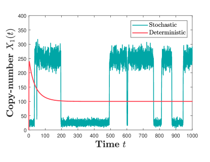
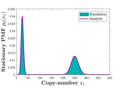
  (a)                                                                          (b)

       

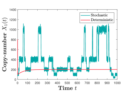
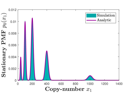
  (c)                                                                          (d)

Figure 1: (a) Representative sample path for the reaction network (16), obtained by applying the Gillespie algorithm (blue-green), together with the deterministic trajectory, obtained by solving equations (22)–(23), in the case the two catalysts satisfy the conservation law $y_{1}(t)+y_{2}(t)=N=M=1$, $\forall t\geq 0$. The initial condition is $(x_{1},y_{1},y_{2})=(0,0,1)$. (b) Stationary $x_{1}$-marginal PMF obtained by the Gillespie algorithm (blue-green histogram) and by the analytic approximation (39) (purple). (c) Analogous results as in panel (a) for the case $y_{1}(t)+y_{2}(t)=N=M=4$, $\forall t\geq 0$, and with the initial condition $(x_{1},y_{1},y_{2})=(800,3,1)$. (d) Analogous results as in panel (b) for the case $y_{1}(t)+y_{2}(t)=N=M=4$, $\forall t\geq 0$. The parameters are fixed to $\alpha_{11}=10^{2}$, $\alpha_{12}=2$, $\alpha_{21}=5\times 10^{2}$, $\beta_{1}=2$, $\gamma_{12}=\gamma_{21}=1$ and $\varepsilon=10^{-2}$.

5.1.2 Multiple-species networks

When considering fast-slow networks with multiple-species auxiliary networks, we focus, for simplicity, on one-species marginal PMFs (as opposed to e.g. the joint PMF). For a given fast-slow network, some marginal PMFs may display unimodality, while others multimodality. There are broadly two reasons why networks of the form (8) may display (marginal) unimodality. Firstly, a marginal PMF may appear unimodal if it takes a significant value at only one mode, i.e. if the weights in (35) take a significant value for only one auxiliary Poissonian. Secondly, the $x_{i}$-marginal PMF $p_{0}(x_{i})$ is unimodal if the underlying Poissonians $\mathcal{P}(x_{i};\,x_{i}^{*})$ from (35) are not well-separated, which occurs under insufficient separation between the deterministic equilibria $x_{i}^{*}$ $=x_{i}^{*}(y_{1}\boldsymbol{\alpha}_{1},y_{2}\boldsymbol{\alpha}_{2},\ldots,y_{n}\boldsymbol{\alpha}_{n},\boldsymbol{\beta})$, $\mathbf{y}\in\pi_{n}^{N}$, of the auxiliary networks. We now provide an example of the extreme case, when the deterministic equilibrium $x_{i}^{*}$ is independent of $\mathbf{y}$ (i.e. all the deterministic equilibria of the auxiliary network coincide), so that $p_{0}(x_{i})$ is a sum of identical Poissonians, and is hence unconditionally unimodal.

       

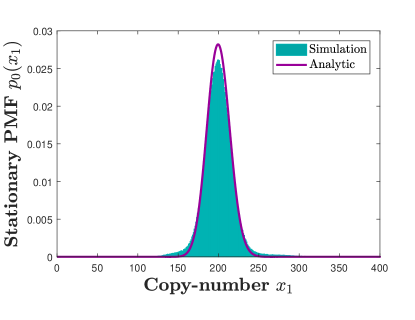
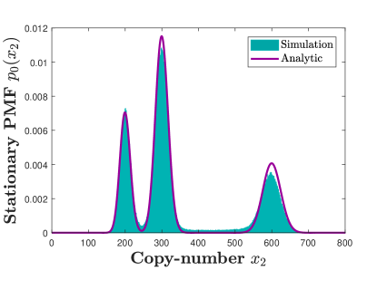
  (a)                                                                          (b)

Figure 2: (a) The stationary $x_{1}$–marginal PMFs of chemical system (40) obtained by the Gillespie algorithm (blue-green histogram) and by analytic approximation (42) (purple solid line), illustrating that species $P_{1}$ from (40) is unimodally distributed, with the mode $x_{1}^{m}=200$. (b) The stationary $x_{2}$–marginal PMFs illustrating that $P_{2}$ has a trimodal distribution, with the modes $x_{2}^{m}\in 10^{2}\times\{2,3,6\}$. The parameters are fixed to $\alpha_{11}=1/2$, $\alpha_{21}=1/6$, $\beta_{1}=1$, $\beta_{2}=2\times 10^{2}$, $\gamma_{12}=\gamma_{21}=1$, $\varepsilon=10^{-2}$ and $N=2$.

Example 5.2

Let us consider the following fast-slow network

$$\mathcal{R}_{\alpha_{1}}:\; G_{1}+P_{2} \xrightarrow[]{\alpha_{11}}G_{1}+P_{1},$$

$$\mathcal{R}_{\alpha_{2}}:\; G_{2}+P_{2} \xrightarrow[]{\alpha_{21}}G_{2}+P_{1},$$

$$\mathcal{R}_{\beta}:\; P_{1} \xrightarrow[]{\beta_{1}}\varnothing,$$

$$\varnothing \xrightarrow[]{\beta_{2}}P_{2},$$

$$\mathcal{R}_{\gamma}^{\varepsilon}:\; G_{1} \xrightleftharpoons[\varepsilon\gamma_{21}]{\varepsilon\gamma_{12}}G_{2},\;\;\;\;\;0<\varepsilon\ll 1,$$ (40)

involving species $\mathcal{P}=(P_{1},P_{2})$ and catalysts $\mathcal{G}=(G_{1},G_{2})$. Species $P_{2}$ may be interpreted as the substrate needed for the gene in both states $G_{1}$ and $G_{2}$ to build the protein $P_{1}$. The auxiliary network $\mathcal{R}_{\delta,\beta}$, with $\boldsymbol{\delta}=(y_{1}\alpha_{11},y_{2}\alpha_{21})$, is given by

$$\mathcal{R}_{\delta_{1}}:\; P_{2} \xrightarrow[]{y_{1}\alpha_{11}}P_{1},$$

$$\mathcal{R}_{\delta_{2}}:\; P_{2} \xrightarrow[]{y_{2}\alpha_{21}}P_{1},$$

$$\mathcal{R}_{\beta}:\; P_{1} \xrightarrow[]{\beta_{1}}\varnothing,$$

$$\varnothing \xrightarrow[]{\beta_{2}}P_{2}.$$ (41)

The deterministic equilibrium of (41) reads

$$\mathbf{x}^{*}=\left(\frac{\beta_{2}}{\beta_{1}},\frac{\beta_{2}}{y_{1}\alpha_{11}+y_{2}\alpha_{21}}\right).$$

In particular, $x_{1}^{*}$ is independent of the catalyst state $\mathbf{y}$. Since (41) is zero-deficient and weakly-reversible, equation (35) is applicable. Summing the equation over $x_{2}$ and $x_{1}$, we respectively obtain

$$p_{0}(x_{1}) =\left(\sum_{\mathbf{y}\in\pi_{2}^{N}}N!\,\frac{(\mathbf{y}^{*}(\boldsymbol{\gamma}))^{\mathbf{y}}}{\mathbf{y}!}\right)\mathcal{P}\!\left(x_{1};\,\frac{\beta_{2}}{\beta_{1}}\right),$$ (42)

$$p_{0}(x_{2}) =\sum_{\mathbf{y}\in\pi_{2}^{N}}\left(N!\,\frac{(\mathbf{y}^{*}(\boldsymbol{\gamma}))^{\mathbf{y}}}{\mathbf{y}!}\right)\mathcal{P}\!\left(x_{2};\,\frac{\beta_{2}}{y_{1}\alpha_{11}+y_{2}\alpha_{21}}\right).$$ (43)

Thus, the stationary $x_{1}$-marginal PMF (42) is independent of $\mathbf{y}$, and always remains unimodal. On the other hand, the stationary $x_{2}$-marginal PMF (43) may display noise-induced multimodality. Hence, the protein $P_{1}$ is unimodally distributed, while the substrate $P_{2}$ may be multimodally distributed. This is also verified in Figure 2 for a particular parameter choice, where one can also notice that (42)–(43) provide an excellent approximation when $\varepsilon=10^{-2}$.

A more complicated reaction network is now presented, involving a second-order auxiliary network.

Example 5.3

Let us consider the following fast-slow network

$$\mathcal{R}_{\alpha_{1}}:\; G_{1} \xrightarrow[]{\alpha_{11}}G_{1}+P_{1},$$

$$\mathcal{R}_{\alpha_{2}}:\; G_{2} \xrightarrow[]{\alpha_{21}}G_{2}+P_{2},$$

$$\mathcal{R}_{\alpha_{3}}:\; G_{3}+P_{1} \xrightarrow[]{\alpha_{31}}G_{3},$$

$$G_{3}+P_{2} \xrightarrow[]{\alpha_{32}}G_{3},$$

$$\mathcal{R}_{\beta}:\; P_{1} \xrightarrow[]{\beta_{1}}\varnothing,$$

$$P_{2} \xrightarrow[]{\beta_{2}}\varnothing,$$

$$P_{1}+P_{2} \xrightleftharpoons[\beta_{6}]{\beta_{3}}P_{3}\xrightleftharpoons[\beta_{5}]{\beta_{4}}P_{2}+P_{4},$$

$$\mathcal{R}_{\gamma}^{\varepsilon}:\; G_{1} \xrightleftharpoons[\varepsilon\gamma_{21}]{\varepsilon\gamma_{12}}G_{2}\xrightleftharpoons[\varepsilon\gamma_{32}]{\varepsilon\gamma_{23}}G_{3},\;\;\;\;\;0<\varepsilon\ll 1,$$ (44)

involving species $\mathcal{P}=(P_{1},P_{2},P_{3},P_{4})$ and catalysts $\mathcal{G}=(G_{1},G_{2},G_{3})$. One may interpret $G_{1},G_{2},G_{3}$ as three possible gene expressions: $G_{1}$ and $G_{2}$ are the producing gene states, creating proteins $P_{1}$ and $P_{2}$, respectively, while $G_{3}$ is a degrading gene state, destroying the two proteins. Molecules $P_{1}$ and $P_{2}$ may also freely decay (without a direct influence of the gene), as well as reversibly form a complex protein $P_{3}$, which may be reversibly converted into a new protein $P_{4}$. Proteins $P_{1}$ and $P_{2}$ may be seen as input molecules (produced by the gene directly), while $P_{3}$ and $P_{4}$ as output of network (44). We are interested in the equilibrium dynamics of protein $P_{4}$.

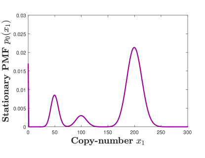
                                         (a)

       

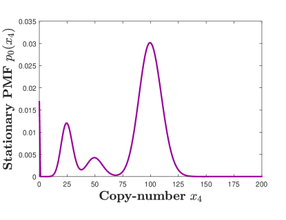
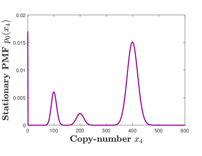
  (b) $\frac{\beta_{3}\beta_{4}}{\beta_{5}\beta_{6}}=\frac{1}{2}$                                                             (c) $\frac{\beta_{3}\beta_{4}}{\beta_{5}\beta_{6}}=2$

Figure 3: (a) The stationary $x_{1}$-marginal PMF of system (44) obtained by analytic approximation (35). The parameters are $\alpha_{11}=10^{2}$, $\alpha_{21}=50$, $\alpha_{31}=1$, $\alpha_{32}=1$, $\beta_{1}=\beta_{2}=\beta_{3}=\beta_{5}=1$, $\beta_{6}=10^{2}$, $\gamma_{12}=\gamma_{32}=1$, $\gamma_{21}=20$, $\gamma_{23}=2$, $\varepsilon=10^{-3}$, $N=2$, and $\beta_{4}=50$. (b) The stationary $x_{4}$-marginal PMF of system (44) given by (46).
(c) The stationary $x_{4}$-marginal PMF of system (44) given by (46) when the value of $\beta_{4}$ is changed to $\beta_{4}=200$ (other parameters are the same as in other panels).

The auxiliary network $\mathcal{R}_{\delta,\beta}$, with $\boldsymbol{\delta}=(y_{1}\alpha_{11},y_{2}\alpha_{21},y_{3}\alpha_{31}$, $y_{3}\alpha_{32})$, is given by $\mathcal{R}_{\delta,\beta}=\mathcal{R}_{\delta_{1}}\cup\mathcal{R}_{\delta_{2}}\cup\mathcal{R}_{\delta_{3}}\cup\mathcal{R}_{\beta},$ where $\mathcal{R}_{\beta}$ is given in (44) and

$$\mathcal{R}_{\delta_{1}}:\; \varnothing \xrightarrow[]{y_{1}\alpha_{11}}P_{1},$$

$$\mathcal{R}_{\delta_{2}}:\; \varnothing \xrightarrow[]{y_{2}\alpha_{21}}P_{2},$$

$$\mathcal{R}_{\delta_{3}}:\; P_{1} \xrightarrow[]{y_{3}\alpha_{31}}\varnothing,$$

$$P_{2} \xrightarrow[]{y_{3}\alpha_{32}}\varnothing.$$

The deficiency of network $\mathcal{R}_{\delta,\beta}$ may be computed using Definition 2.5: $|\mathcal{C}|=6$, $\ell=2$ and $s=4$, so that it is a zero-deficient network, which is also reversible. The deterministic equilibrium reads:

$$\mathbf{x}^{*}=\left(\frac{y_{1}\alpha_{11}}{y_{3}\alpha_{31}+\beta_{1}},\frac{y_{2}\alpha_{21}}{y_{3}\alpha_{32}+\beta_{2}},\frac{\beta_{3}}{\beta_{6}}x_{1}^{*}x_{2}^{*},\frac{\beta_{3}\beta_{4}}{\beta_{5}\beta_{6}}x_{1}^{*}\right).$$ (45)

It follows from (35) and (45) that the equilibrium behaviour of proteins $P_{3}$ and $P_{4}$, which are produced by the gene indirectly (via $P_{1}$ and $P_{2}$), is captured by

$$p_{0}(x_{3}) =\sum_{\mathbf{y}\in\pi_{3}^{N}}\left(N!\,\frac{(\mathbf{y}(\boldsymbol{\gamma})^{*})^{\mathbf{y}}}{\mathbf{y}!}\right)\mathcal{P}\!\left(x_{3};\,\frac{\beta_{3}}{\beta_{6}}x_{1}^{*}x_{2}^{*}\right),$$

$$p_{0}(x_{4}) =\sum_{\mathbf{y}\in\pi_{3}^{N}}\left(N!\,\frac{(\mathbf{y}(\boldsymbol{\gamma})^{*})^{\mathbf{y}}}{\mathbf{y}!}\right)\mathcal{P}\!\left(x_{4};\,\frac{\beta_{3}\beta_{4}}{\beta_{5}\beta_{6}}x_{1}^{*}\right).$$ (46)

One can notice from (46) that, for each gene state $\mathbf{y}\in\pi_{3}^{N}$, the mode of the complex protein $P_{3}$ is given by the product of the modes of $P_{1}$ and $P_{2}$ scaled by a factor $\beta_{3}/\beta_{6}$. In particular, when there is only one copy of the gene, $N=1$, so that $x_{1}^{*}x_{2}^{*}=0$, it follows that the PMF of $P_{3}$ is unimodal, and approaches the Kronecker-delta function centered at zero as $\varepsilon\to 0$. On the other hand, modes of $P_{4}$ are modes of $P_{1}$ scaled by a factor $\beta_{3}\beta_{4}/(\beta_{5}\beta_{6})$. This is also illustrated in Figure 3, where we fix $N=2$, and display the stationary $x_{1}$-marginal PMF in Figure 3(a), while $x_{4}$-marginal PMF with $\beta_{3}\beta_{4}/(\beta_{5}\beta_{6})=1/2$ in Figure 3(b), and with $\beta_{3}\beta_{4}/(\beta_{5}\beta_{6})=2$ in Figure 3(c). One can notice that the modes of $p_{0}(x_{4})$ are contracted, and dilated, by a factor of two in Figures 3(b), and 3(c), respectively, when compared to $p_{0}(x_{1})$. Let us note that, for this parameter change, only the plotted stationary $x_{4}$-marginal PMF changes, while the other one-species marginal PMFs remain the same, because they are independent of $\beta_{4}$.

5.2 Stochastic multicyclicity

In this section, we present a fast-slow network with auxiliary network that exhibits multimodality and stochastic oscillations, which we have constructed using (34). In this case, in contrast to Section 5.1, the auxiliary PMFs are not Poissonians (more generally, Theorem 2.2 is not applicable). The resulting fast-slow network displays an arbitrary number of noisy limit cycles (known as stochastic multicyclicity [29]), and may illustrate the kind of stochastic dynamics arising when a gene produces a protein whose concentration oscillates in time.

Example 5.4

Let us consider the following fast-slow network

$$\mathcal{R}_{\alpha_{1}}:\; G_{1}+2P_{2} \xrightarrow[]{\alpha_{11}}G_{1}+P_{1}+P_{2},$$

$$\mathcal{R}_{\beta}:\; \varnothing \xrightleftharpoons[\beta_{2}]{\beta_{1}}P_{2},$$

$$P_{2} \xrightarrow[]{\beta_{3}}P_{1},$$

$$P_{1}+2P_{2} \xrightarrow[]{\beta_{4}}3P_{2},$$

$$\mathcal{R}_{\gamma}^{\varepsilon}:\; G_{1} \xrightleftharpoons[\varepsilon\gamma_{21}]{\varepsilon\gamma_{12}}G_{2},\;\;\;\;\;0<\varepsilon\ll 1.$$ (47)

Subnetwork $\mathcal{R}_{\alpha_{1}}$ may be seen as a caricature of the gene, in state $G_{1}$, creating products which bind two proteins $P_{2}$ and then converting one of them to a new protein $P_{1}$. Subnetwork $\mathcal{R}_{\beta}$ is the biochemical oscillator known as the Brusselator [30], here describing interactions between the two proteins.

The auxiliary network $\mathcal{R}_{\delta,\beta}$, with $\delta_{1}=y_{1}\alpha_{11}$, is given by $\mathcal{R}_{\delta,\beta}=\mathcal{R}_{\delta_{1}}\cup\mathcal{R}_{\beta},$ where $\mathcal{R}_{\beta}$ is given in (47) and

$$\mathcal{R}_{\delta_{1}}:\;2P_{2}\xrightarrow[]{y_{1}\alpha_{11}}P_{1}+P_{2},$$ (48)

Note that $\mathcal{R}_{\delta,\beta}$ is not zero-deficient (nor weakly-reversible), so that (35) is not applicable. We set $\beta_{1}=\beta_{2}=\beta_{4}=1$ and $\beta_{3}=10$ in the following analysis and in Figure 4.

       

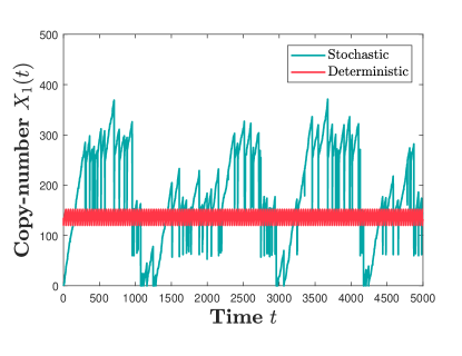
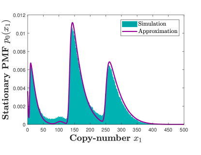
  (a)                                                                          (b)

       

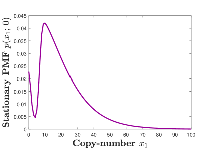
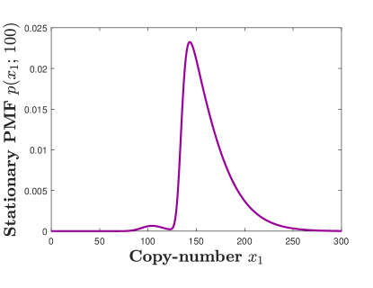
  (c)                                                                          (d)

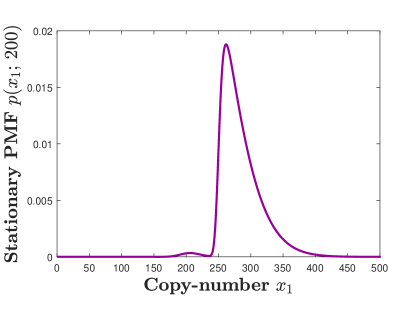
                                         (e)

Figure 4: (a) A representative sample path for network (47) (blue-green), together with the deterministic trajectory, obtained by numerically solving (49) (purple solid line). The parameters are $\alpha_{11}=10^{2}$, $\beta_{1}=\beta_{2}=\beta_{4}=1$, $\beta_{3}=10$, $\gamma_{12}=1$, $\gamma_{21}=3/2$, $\varepsilon=10^{-3}$, and $N=2$.
(b) The stationary $x_{1}$-marginal PMF of (47) (blue-green histogram) and its approximation given by (50) (purple solid line).
(c)–(e) The stationary $x_{1}$-marginal PMFs of the underlying auxiliary network given in (50), when: (c) $y_{1}=0$; (d) $y_{1}=1$; and (e) $y_{2}=2$.

Deterministic analysis.The RREs of the auxiliary network, with the concentration of catalyst $G_{1}$ set to its equilibrium value $y_{1}^{*}$, given in (24), read

$$\frac{\mathrm{d}x_{1}}{\mathrm{d}t} =10x_{2}-(x_{1}-y_{1}^{*}\alpha_{11})\,x_{2}^{2},$$

$$\frac{\mathrm{d}x_{2}}{\mathrm{d}t} =1-11x_{2}+(x_{1}-y_{1}^{*}\alpha_{11})\,x_{2}^{2}.$$ (49)

System (49) has a unique equilibrium $(x_{1}^{*},x_{2}^{*})=(10+y_{1}^{*}\alpha_{11},1)$, which is unstable, and surrounded by a unique stable limit cycle, for the parameters chosen in our paper [30]. Deterministically, the only effect reaction $\mathcal{R}_{\delta_{1}}$ has on Brusselator $\mathcal{R}_{\beta}$ is to simply translate its equilibrium and limit cycle by $y_{1}\alpha_{11}$. Hence, qualitative properties of the equilibrium and limit cycle are independent of the values of $y_{1}$ and $\alpha_{11}$. Fixing $\alpha_{11}=10^{2}$, the conservation constants $N=M=2$, and coefficients $\gamma_{12}=1$, $\gamma_{21}=3/2$, gives the equilibrium $(x_{1}^{*},x_{2}^{*})=(130,1)$. In Figure 4(a), we show in red the $x_{1}$-solution of the RREs underlying (47) for a given initial condition, and one can notice the time-oscillations.

Stochastic analysis. Applying (34) on reaction network (47), it follows that, for sufficiently small $\varepsilon$, the stationary $x_{1}$-marginal PMF is approximately given by

$$p_{0}(x_{1}) =\left(\frac{\gamma_{12}}{\gamma_{12}+\gamma_{21}}\right)^{2}p(x_{1};\,0)+\frac{2\gamma_{12}\gamma_{21}}{(\gamma_{12}+\gamma_{21})^{2}}\,p(x_{1};\,\alpha_{11})+\left(\frac{\gamma_{21}}{\gamma_{12}+\gamma_{21}}\right)^{2}p(x_{1};\,2\alpha_{11})$$

$$=\frac{4}{25}\,p(x_{1};\,0)+\frac{12}{25}\,p(x_{1};\,100)+\frac{9}{25}\,p(x_{1};\,200),$$ (50)

where $p(x_{1};\,y_{1}\alpha_{11})$ is the auxiliary PMF.

In Figure 4(a), we display in blue-green a representative sample path of (47), which appears to switch between three noisy limit cycles, one of which is close to the deterministic limit cycle. To gain more insight, in Figures 4(c)–4(e), the auxiliary PMFs $p(x_{1};\,0)$, $p(x_{1};\,100)$ and $p(x_{1};\,200)$ from (50) are presented, respectively, obtained by numerically solving the two-species CME for auxiliary network $\mathcal{R}_{\delta,\beta}=\mathcal{R}_{\delta_{1}}\cup\mathcal{R}_{\beta}$ given in (47) and (48). In all the three cases, the underlying deterministic model displays only one stable set - the limit cycle, while the auxiliary PMFs are bimodal. In Figure 4(b), we present as the blue-green histogram the $x_{1}$-marginal PMF obtained from simulations, and as the purple curve the analytic approximation given by the weighted sum (50). One can notice a good match for $\varepsilon=10^{-3}$ taken in Figure 4. In addition to the three modes where the PMF takes largest values, there are two other modes (one at $0$, and one near $100$), arising from $p(x_{1};\,0)$ and $p(x_{1};\,100)$. On the other hand, the second mode of $p(x_{1};\,200)$, appearing near $200$ in Figure 4(e), is merged with $p(x_{1};\,100)$ for the particular choice of the parameters. Let us note that, while the stationary $x_{1}$-marginal PMF displays multimodality, the stationary $x_{2}$-marginal PMF is unimodal and concentrated around $0$. This results from the fact that $X_{2}(t)$ spends most of the time near zero for each of the three noisy limit cycles.

More generally, taking the conservation constant $N\geq 0$, network (47) may display $(N+1)$ distinct noisy limit cycle. Moreover, replacing the slow subnetwork

$$G_{1}\xrightleftharpoons[\varepsilon\gamma_{21}]{\varepsilon\gamma_{12}}G_{2},\qquad\mbox{from~{}{\rm(\ref{eq:fastslow4})} by}\qquad G_{1}\xrightleftharpoons[\varepsilon\gamma_{01}]{\varepsilon\gamma_{10}}\varnothing$$

(which relaxes Assumption 3.2, see also Section 6 for a discussion), the resulting fast-slow network may display an infinite number of noisy limit cycles.

6 Summary and conclusion

In this paper, we have introduced a class of chemical reaction networks under mass-action kinetics, involving two time-scales and catalytic species, and inspired by gene-regulatory networks [15], whose deterministic and stochastic descriptions display ‘deviant’ differences [9]. More precisely, fast-slow networks of the form (8)–(9), under three Assumptions 3.1– 3.3, as defined in Section 3, have been considered. By analyzing the underlying dynamical models in Section 4, we have identified a novel stochastic phenomenon causing the qualitative differences between the deterministic and stochastic models. In particular, it is shown that, as a result of the conversions among the catalysts (genes) in the slow subnetwork, the fast species (proteins) have a probability distribution which is a mixture of the probability distributions of modified fast subnetworks, called auxiliary networks, which are obtained if the catalysts are ‘stripped-off’. We call this phenomeon noise-induced mixing, and it is captured in the central result in this paper: equation (34), which was obtained by applying first-order perturbation theory on the underlying singularly perturbed CME.

In Section 5, we have applied the result to investigate multimodality in the context of systems biology. In Section 5.1, fast-slow reaction networks with auxiliary networks under suitable constraints (zero-deficiency and weak-reversibility) were considered, allowing for analytic results. It is shown in Lemma 5.1 that, under these constraints, while the deterministic model is always unistable, the stochastic model may display multimodality. When the auxiliary networks involve only one species and first-order reactions, we also derived bounds on the modes, given as Lemma 5.2. When the auxiliary networks involve multiple species, we discuss, and demonstrate via examples (40) and (44), that some species may be unimodal, while other multimodal, and that modes of different species are generally coupled. In Section 5.2, a reaction network involving an oscillator is presented, capturing the kind of behaviour which may arise in gene-regulatory networks involving proteins whose concentrations oscillate in time. We show that, as a result of noise-induced mixing, the reaction network may display stochastic multimodality, where the modes correspond to copies of the underlying unique deterministic limit cycle, thus also showing that gene-regulatory networks, involving as few as three species, may display an arbitrary number of noisy limit cycles. It was also demonstrated that result (34) is beneficial for numerical simulations - instead of simulating the higher-dimensional stiff dynamics of the fast-slow networks, involving the small parameter $\varepsilon$, one may instead simulate the underlying lower-dimensional auxiliary networks and use (34) (see also [23, 24, 31, 32] for discussions on simulating general fast-slow networks).

Three Assumptions 3.1–3.3 have been made in this paper to facilitate the analysis. However, noise-induced mixing occurs in a broader class of reaction networks. For example, we may relax the assumptions about the catalysing network, made in Assumption 3.2, in the following two ways. Firstly, we may allow the slow subnetwork $\mathcal{R}_{\gamma}^{\varepsilon}(\mathcal{G})$ to be open, in which case the multinomial function (33), appearing as $\mathbf{x}$-independent weights in (34), is replaced with the Poissonian function of the form (6). Secondly, we may consider the more general regulated slow subnetworks, $\mathcal{R}_{\gamma}^{\varepsilon}(\mathcal{P},\mathcal{G})$, describing gene-regulatory networks with feedback [15]. In this case, the derivation from Section 4.2 remains valid under one modification: the RHS of the effective CME (32) depends on the moments of the fast species $\mathbf{x}$ (proteins) with respect to the auxiliary PMF, which themselves depend on the catalysts (genes) $\mathbf{y}$. As a consequence, the weights from (34) then generally have a different form. However, the auxiliary PMFs ($\mathbf{x}$-dependent factors from (34)) remain unchanged, so that noise-induced mixing remains to operate. Put more simply, proteins in the discussed gene-regulatory networks with and without feedback have approximately the same modes, but the height of the probability distribution at the modes is generally different. Note that networks (8)–(9) experience, not only long-term, but also transient noise-induced mixing: if the time-dependent PMF $p_{0}(\mathbf{y},\tau)$, satisfying (32), is substituted into (34), one obtains an approximation to the time-dependent marginal PMF, $p_{0}(\mathbf{x},\tau)$, which has the same form as (34), but with suitable time-dependent weights.

Finally, let us note that noise-induced mixing may also be applicable to the field of synthetic biology, which aims to design reaction systems with predefined behaviours [13]. In particular, given a target probability distribution, one may construct a suitable fast-slow network, such that its probability distribution, given by (34), approximates the target one.

7 Acknowledgements

This work was supported by NIH Grant $\#29123$ and a Visiting Research Fellowship from Merton College, Oxford, awarded to Hans Othmer. Radek Erban would also like to thank the Royal Society for a University Research Fellowship.

References

- [1] Kuthan, H. (2001) Self-organisation and orderly processes by individual protein complexes in bacterial cell. Progress in Biophysics and Molecular Biology 75(1-2): 1–17.
- [2] Spudich, J. L., Koshland, Jr. D. E. (1976) Non-genetic individuality: chance in the single cell. Nature 262: 467–471.
- [3] Ozbudak, E. M., Thattai, M., Kurtser, I., Grossman, A. D., van Oudenaarden, A. (2002) Regulation of noise in the expression of a single gene. Nature Genetics 31(1): 69–73.
- [4] Levsky, J. M., Singer, R. H. (2003) Gene expression and the myth of the average cell. Trends Cell Biol 13(1): 4–6.
- [5] Raj, A., van Oudenaarden, A. (2008) Nature, nurture, or chance: stochastic gene expression and its consequences. Cell 135(2): 216–226.
- [6] Fraser, D., Kaern, M. (2009) A chance at survival: gene expression noise and phenotypic diversification strategies. Molecular microbiology 71(6): 1333–1340.
- [7] Senecal, A., Munsky, B., Proux, F., Ly, N., Braye, F. E., Zimmer, C., Mueller, F., Darzacq, X. (2014) Transcription factors modulate c-fos transcriptional bursts. Cell reports 8(1): 75–83.
- [8] Wickramasinghe, V. O, Laskey, R. A. (2015) Control of mammalian gene expression by selective mRNA export. Nature Reviews Molecular Cell Biology 16(7): 431–442.
- [9] Samoilov, M. S., Arkin, A. P. (2006) Deviant effects in molecular reaction pathways. Nature Biotechnology 24(10): 1235–1240.
- [10] Kuwahara, H., Gao, X. (2013) Stochastic effects as a force to increase the complexity of signaling networks. Scientific reports, 3.
- [11] Erban, R., Chapman, J., Kevrekidis, I., Vejchodský, T. (2009) Analysis of a stochastic chemical system close to a SNIPER bifurcation of its mean-field model. SIAM Journal on Applied Mathematics 70(3): 984-1016.
- [12] Liao, S., Vejchodský, T., Erban, R. (2015) Tensor methods for parameter estimation and bifurcation analysis of stochastic reaction networks. Journal of the Royal Society Interface 12(108): 20150233.
- [13] Plesa, T., Zygalakis, K., Anderson, D. F., Erban, R. (2018) Noise Control for DNA Computing. Available as https://arxiv.org/abs/1705.09392.
- [14] Érdi, P., Tóth, J. (1989) Mathematical Models of Chemical Reactions. Theory and Applications of Deterministic and Stochastic Models. Manchester University Press, Princeton University Press.
- [15] Kepler, T. B., Elston, T. C. (2001) Stochasticity in transcriptional regulation: Origins, consequences, and mathematical representations. Biophysical Journal 81: 3116–3136.
- [16] Duncan, A., Liao, S., Vejchodský, T., Erban, R., Grima, R. (2015) Noise-Induced Multistability in Chemical Systems: Discrete vs Continuum Modelling. Physical Review E 91, 042111.
- [17] Feinberg, M. (1979) Lectures on Chemical Reaction Networks. Lecture Notes, Mathematics Research Center, University of Wisconsin.
- [18] Othmer, H. G. (1981) A graph-theoretic analysis of chemical reaction networks. Lecture Notes, Rutgers University.
- [19] Anderson, D. F., Kurtz, T. G. (2015) Stochastic analysis of biochemical systems. Springer.
- [20] Gadgil, C., Lee, C. H., Othmer, H. G. (2005) A stochastic analysis of first-order reaction networks. Bulletin of Mathematical Biology 67(5): 901–946.
- [21] Craciun, G. (2015) Toric Differential Inclusions and a Proof of the Global Attractor Conjecture. Available as http://arxiv.org/abs/1501.02860.
- [22] Van Kampen, N. G. (2007) Stochastic Processes in Physics and Chemistry. Elsevier.
- [23] Kan, X., Lee, C. H., Othmer, H. G (2016) A multi-time-scale analysis of chemical reaction networks: II Stochastic systems. Journal of Mathematical Biology 73: 1081–1129.
- [24] Cotter, S., Zygalakis, K., Kevrekidis, I., Erban, R. (2011) A constrained approach to multiscale stochastic simulation of chemically reacting systems. Journal of Chemical Physics 135(9), 094102.
- [25] Cotter, S., Vejchodský, T., Erban, R. (2013) Adaptive finite element method assisted by stochastic simulation of chemical systems. SIAM Journal on Scientific Computing 35(1), pp. B107-B131.
- [26] Anderson, D. F., Craciun, G., Kurtz, T. G. (2010) Product-form stationary distributions for deficiency zero chemical reaction networks. Bulletin of Mathematical Biology 72(8): 1947–1970.
- [27] Pavliotis, G. A., Stuart, A. M. (2008) Multiscale Methods: Averaging and Homogenization. Springer, New York.
- [28] Gillespie, D. T. (1977) Exact stochastic simulation of coupled chemical reactions. Journal of Physical Chemistry 81(25): 2340–2361.
- [29] Plesa, T., Vejchodský, T., Erban, R. (2017) Test Models for Statistical Inference: Two-Dimensional Reaction Systems Displaying Limit Cycle Bifurcations and Bistability, in Stochastic Dynamical Systems, Multiscale Modeling, Asymptotics and Numerical Methods for Computational Cellular Biology. Springer.
- [30] Prigogine, I., and Lefever, R. (1968) Symmetry breaking instabilities in dissipative systems, II. Journal of Chemical Physics 48(4): 1695–1700.
- [31] Erban, R., Kevrekidis, I., Adalsteinsson, D., Elston, T. (2006) Gene regulatory networks: a coarse-grained, equation-free approach to multiscale computation. Journal of Chemical Physics 124(8): 084106.
- [32] Cotter, S., Erban, R. (2016) Error analysis of diffusion approximation methods for multiscale systems in reaction kinetics. SIAM Journal on Scientific Computing 38(1), pp. B144-B163.