Dissipative tunnelling by means of scaled trajectories

Abstract

Dissipative quantum tunnelling through an inverted parabolic barrier is considered in the presence of an electric field. ​A Schrödinger-Langevin or Kostin quantum-classical transition wave equation is used and applied resulting in a scaled differential equation of motion. A Gaussian wave packet solution to the resulting scaled Kostin nonlinear equation is assumed and compared to the same solution for the scaled linear Caldirola-Kanai equation. The resulting scaled trajectories are obtained at different dynamical regimes and friction cases, showing the gradual decoherence process in this open dynamics. Theoretical results show that the transmission probabilities are always higher in the Kostin approach than in the Caldirola-Kanai approach in the presence or not of an external electric field. This discrepancy should be understood due to the presence of an environment since the corresponding open dynamics should be governed by nonlinear quantum equations, whereas the second approach is issued from an effective Hamiltonian within a linear theory.

I Introduction

Dissipative tunnelling in the presence or not of an electric field has many applications in transport properties, reactive scattering, quantum optics, molecular biology, etc. One of the main goals is to analyze the gradual decoherence process existing in this particular dynamics by using very different theoretical methods within the density matrix, path-integral and Langevin formalisms Weiss-book-1999 ; Razavy-book-2005 . A new alternative way which is by far much less used is the Bohmian formalism NaMi-book-2017 where the decoherence process is described in terms of trajectories leading, in our opinion, to a more intutitive way of understanding it. In this sense, dealing with analytically solvable models is very useful in order to gain new insights.

By considering dissipation from a phenomenological way, the tunnelling dynamics by an inverted parabollic barrier is very convenient because it provides all the main ingredients to tackle with success such an endeavour as well as to compare with existing results coming from different theoretical treatments. In particular, comparison with the works by Baskoutas and Jannussis BaJa-JPA-1992 and Papadopoulos Pa-JPA-1997 . Our purpose is to analyze two different approaches to this dissipative dynamics, the nonlinear, logarithmic Schrödinger-Langevin (or Kostin) equation Kostin-1972 and the linear Schrödinger equation coming from the so-called Cardirola-Kanai Hamiltonian caldirola ; kanai ; SaCaRoLoMi-AP-2014 ; MoMi-JPCO-2018 within the Bohmian formalism Holland-book-1993 ; salva1 ; salva2 . Recently, Tokieda and Hagino ToHa-PRC-2017 have considered the same approaches to study dissipative tunneling without the presence of an electrical field by solving directly the corresponding wave equations. The gradual decoherence process is better studied by using the so-called quantum-classical transition wave equation, originally proposed by Richardson et al. RiSchMaVaBa-PRA-2014 in the context of conservative systems. This quantum-classical transition is governed by a continuous parameter covering these two regimes as being the two extreme cases. Recently, Chou has applied this wave equation to analyze wave-packet interference Chou1-2016 and the dynamics of the harmonic and Morse oscillators with complex trajectories Chou2-2016 . Here, we have extended this procedure to dissipative quantum dynamics. Doing this, we have a wave equation even in the classical regime and the Born rule is assumed in this regime too. Then, by considering the actual momentum Holland-book-1993 distribution function of particles in the classical ensemble, we have a strict answer to the question of classical phase space distribution function which is problematic otherwise HoPaBa-JPA-2009 . The resulting trajectories have been called scaled trajectories MoMi-JPCO-2018 since a scaled Planck’s constant in terms of that parameter is used. Furthermore, by assuming a time-dependent Gaussian ansatz for the probability density, theses scaled trajectories are written as a sum of a classical trajectory (a particle property) plus a term containing the width of the corresponding wave packet (a wave property) within of what has been called dressing scheme NaMi-book-2017 . In the quantum regime, the corresponding trajectories are the well-known quantum trajectories due to Bohm which display the noncrossing property which, in general, is no longer valid in the classical regime but it is kept in the transtion regime. However, in this work, this property is still valid in the classical regime by construction of the transition wave equation itself. This new aspect together with the Born rule for the distribution of particles’ position in the classical ensemble lead us to have a good criterium for tunnelling.

The procedure of using a continuous parameter monitoring the different regimes in the theory (a scaled Planck’s constant) is apparently quite similar to the WKB approach (a series expansion in powers of Planck’s constant), widely used in conservative systems. However, there are several important differences. First, in the WKB, the classical Hamilton-Jacobi equation for the classical action at zero order of the expansion in powers of $\hbar$ is obtained whereas, in the scaling procedure, the so-called classical wave (nonlinear) equation Schi-PR-1962 is reached by construction. Second, the hierarchy of the differential equations for the action at different orders of the expansion in $\hbar$ is substituted by only a transition wave equation which can be easily solved in the linear domain. Third, in the Bohmian framework, the transition from quantum to classical trajectories is carried out in a continuous way allowing us to follow the continuity of the trajectories when changing of regime. Fourth, the scaling procedure extended and applied to open (dissipative and/or stochastic) quantum systems is very easy to implement. And fifth, the gradual decoherence process due to the scaled Planck’s constant can be seen as an extra source which it has to be added to the decoherence due to the presence of an environment.

The organization of this work is as follows. In Section II, the nonlinear (logarithmic) Schrödinger-Langevin or Kostin equation within the context of open quantum systems as well as the corresponding scaled equation are introduced. They are then specialized to the dissipative case. In Section III, the Cardirola-Kanai formalism, where dissipation is introduced from a phenomenological point of view, is developed leading to a linear Schrödinger equation. Section IV deals with the dissipative Bohmian dynamics and scaled trajectories by assuming a time-dependent Gaussian ansatz for the probability density. The presence of the field in this dissipative tunnelling dynamics is considered in Section V. Finally, results and discussion as well as some conclusions are presented in the remaining two sections.

II Quantum-classical transition and scaled Schrödinger-Langevin equations

Kostin derived heuristically from the standard Langevin equation the so-called Schrödinger-Langevin or Kostin nonlinear (logarithmic) equation which is written in one dimension as Kostin-1972 ; NaMi-book-2017

$$i\hbar\frac{\partial}{\partial t}\psi(x,t) = \left[-\frac{\hbar^{2}}{2m}\frac{\partial^{2}}{\partial x^{2}}+V(x,t)+V_{r}(x,t)+\frac{\gamma\hbar}{2i}\left(\ln\frac{\psi}{\psi^{*}}-\left\langle\ln\frac{\psi}{\psi^{*}}\right\rangle\right)\right]\psi(x,t),$$ (1)

where $m$ is the mass of the quantum particle, $\gamma$ the friction coefficient, $V(x)$ is the interaction potential and $V_{r}(x)$ the random potential given by

$$V_{r}(x,t) = x~{}F_{r}(t),$$ (2)

$F_{r}(t)$ being a time-dependent random force. Following RiSchMaVaBa-PRA-2014 , Eq. (1) can be rewritten as a quantum-classical transition wave equation as follows

$$i\hbar\frac{\partial}{\partial t}\psi_{\epsilon}(x,t) = \bigg{[}-\frac{\hbar^{2}}{2m}\frac{\partial^{2}}{\partial x^{2}}+V(x,t)+V_{r}(x,t)+\frac{\gamma\hbar}{2i}\left(\ln\frac{\psi_{\epsilon}}{\psi_{\epsilon}^{*}}-\left\langle\ln\frac{\psi_{\epsilon}}{\psi_{\epsilon}^{*}}\right\rangle\right)$$ (3)

$$~{}~{}+(1-\epsilon)\frac{\hbar^{2}}{2m}\frac{1}{|\psi_{\epsilon}(x,t)|}\frac{\partial^{2}|\psi_{\epsilon}(x,t)|}{\partial x^{2}}\bigg{]}\psi_{\epsilon}(x,t),$$

where a degree of quantumness given by the $\epsilon$ parameter, with $0\leq\epsilon\leq 1$, is included by means of an extra sum representing the quantum potential of the corresponding Bohmian dynamics Holland-book-1993 ; NaMi-book-2017 ,

$$Q_{\epsilon}(x,t) = -\frac{\hbar^{2}}{2m}\frac{1}{|\psi_{\epsilon}(x,t)|}\frac{\partial^{2}|\psi_{\epsilon}(x,t)|}{\partial x^{2}}.$$ (4)

This equation provides a continuous or gradual description for the transition process of physical systems from purely quantum, $\epsilon=1$, to purely classical, $\epsilon=0$, regime which is ruled by the so-called classical wave equation Schi-PR-1962 . This parameter can also be seen as one defining the dynamical regime. The wave function $\psi_{\epsilon}(x,t)$ is thus affected by this parameter determining this transition or decoherence proces. By substituting now the polar form of this wave function

$$\psi_{\epsilon}(x,t) = R_{\epsilon}(x,t)e^{iS_{\epsilon}(x,t)/\hbar}$$ (5)

into the transition wave equation (3), the following coupled equations for the amplitude $R_{\epsilon}(x,t)$ and phase $S_{\epsilon}(x,t)$ are obtained

$$\frac{\partial R_{\epsilon}}{\partial t} = -\frac{1}{2m}\left(2\frac{\partial R_{\epsilon}}{\partial x}\frac{\partial S_{\epsilon}}{\partial x}+R_{\epsilon}\frac{\partial^{2}S_{\epsilon}}{\partial x^{2}}\right),$$ (6)

$$-\frac{\partial S_{\epsilon}}{\partial t}R_{\epsilon} = -\frac{\hbar^{2}}{2m}\left[\epsilon\frac{\partial^{2}R_{\epsilon}}{\partial x^{2}}-\frac{1}{\hbar^{2}}R_{\epsilon}\left(\frac{\partial S_{\epsilon}}{\partial x}\right)^{2}\right]+\bigg{[}V(x,t)+V_{r}(x,t)+\gamma(S_{\epsilon}-\langle S_{\epsilon}\rangle)\bigg{]}R_{\epsilon},$$ (7)

and where we have made use of the fact that

$$S_{\epsilon} = \frac{\hbar}{2i}\ln\frac{\psi_{\epsilon}}{\psi_{\epsilon}^{*}}.$$ (8)

Furthermore, by introducing the so-called scaled Plank’s constant as

$$\tilde{\hbar} = \hbar~{}\sqrt{\epsilon},$$ (9)

and the corresponding scaled wave function as

$$\tilde{\psi}(x,t) = R_{\epsilon}(x,t)e^{iS_{\epsilon}(x,t)/\tilde{\hbar}},$$ (10)

into Eqs. (6) and (7) and, after some straightforward algebraic manipulations, the following scaled nonlinear Schrödinger-Langevin equation for a stochastic dynamics is again reached

$$i\tilde{\hbar}\frac{\partial}{\partial t}\tilde{\psi}(x,t) = \left[-\frac{\tilde{\hbar}^{2}}{2m}\frac{\partial^{2}}{\partial x^{2}}+V(x,t)+V_{r}(x,t)+\frac{\gamma\tilde{\hbar}}{2i}\left(\ln\frac{\tilde{\psi}}{\tilde{\psi}^{*}}-\left\langle\ln\frac{\tilde{\psi}}{\tilde{\psi}^{*}}\right\rangle\right)\right]\tilde{\psi}(x,t),$$ (11)

$\tilde{\psi}(x,t)$ being the scaled wave function. When the random potential $V_{r}(x,t)$ is neglected, the dissipative system is described by

$$i\tilde{\hbar}\frac{\partial}{\partial t}\tilde{\psi}(x,t) = \left[-\frac{\tilde{\hbar}^{2}}{2m}\frac{\partial^{2}}{\partial x^{2}}+V(x,t)+\frac{\gamma\tilde{\hbar}}{2i}\left(\ln\frac{\tilde{\psi}}{\tilde{\psi}^{*}}-\left\langle\ln\frac{\tilde{\psi}}{\tilde{\psi}^{*}}\right\rangle\right)\right]\tilde{\psi}(x,t),$$ (12)

being again a nonlinear logarithmic equation, the scaled Kostin equation. In any case, the transition wave equation (3) is equivalent to the scaled nonlinear Schödinger-Langevin equation (11) (or (12) only for the dissipative case). Moreover, the corresponding wave functions and phases are related by

$$\tilde{\psi}(x,t) = \psi_{\epsilon}(x,t)\exp\left[\frac{i}{\hbar}\left(\frac{1}{\sqrt{\epsilon}}-1\right)S_{\epsilon}(x,t)\right],$$ (13)

which are derived from Eqs. (5) and (10).

Thus, the decoherence process resulting from the open quantum dynamics and scaled Planck’s constant is carried out in a gradual way (it is worth mentioning that the environment is also seen as acting like a continuous measuring apparatus).

III Quantum-classical transition and scaled Schrödinger equations in the CK approach

The so-called classical CK Hamiltonian for dissipative systems is given by Razavy-book-2005

$$H=\frac{p^{2}}{2m}e^{-\gamma t}+V(x)e^{\gamma t}$$ (14)

and its corresponding Hamiltonian operator $\hat{H}$ can be obtained from the standard quantization rule by substituting the momentum $p$ by $\frac{\hbar}{i}\frac{\partial}{\partial x}$,

$$\hat{H} = -\frac{\hbar^{2}}{2m}e^{-\gamma t}\frac{\partial^{2}}{\partial x^{2}}+e^{\gamma t}V(x).$$ (15)

It is well known that the commutation relation of the position and kinematic momentum operators is given by $[x,p]=i\hbar e^{-\gamma t}$, leading to the violation of the Heisenberg uncertainty principle. By means of the transformation to the canonical variables ${\bar{x}}=x$ and ${\bar{p}}=pe^{\gamma t}$, this principle is again fulfilled. Notice that as long as quantities related to the kinematic momentum are not computed, the use of the corresponding wave equation in the coordinate space is formally correct SaCaRoLoMi-AP-2014 . In this framework, friction shows the action of an effective (almost macroscopic) environment coupled to the particle making the motion more and more predictable (classical) as time proceeds. Thus, the violation of the uncertainty principle has sometimes been justified from a dissipative dynamics Pa-JPA-1997 . The time-dependent Schrödinger equation within the CK framework then reads as

$$i\hbar\frac{\partial}{\partial t}\psi(x,t) = \left[-\frac{\hbar^{2}}{2m}e^{-\gamma t}\frac{\partial^{2}}{\partial x^{2}}+e^{\gamma t}V(x)\right]\psi(x,t).$$ (16)

Following now the same procedure as in previous Section, a quantum-classical transition wave equation RiSchMaVaBa-PRA-2014 can again be introduced according to MoMi-JPCO-2018 as

$$i\hbar\frac{\partial}{\partial t}\psi_{\epsilon}(x,t) = \left[-\frac{\hbar^{2}}{2m}e^{-\gamma t}\frac{\partial^{2}}{\partial x^{2}}+V(x)e^{\gamma t}+(1-\epsilon)\frac{\hbar^{2}}{2m}\frac{1}{|\psi_{\epsilon}(x,t)|}\frac{\partial^{2}|\psi_{\epsilon}(x,t)|}{\partial x^{2}}e^{-\gamma t}\right]\psi_{\epsilon}(x,t),$$ (17)

This equation also provides a continuous or gradual description for the transition or decoherence process of physical systems from purely quantum to classical regime in the CK framework. Then, by substituting the standard polar form of the wave function given by Eq. (5) into Eq. (17) and after some straightforward manipulations, the following coupled equations are reached

$$-\frac{\partial S_{\epsilon}}{\partial t}\tilde{\psi} = \frac{1}{2m}e^{-\gamma t}\left(\frac{\partial S_{\epsilon}}{\partial x}\right)^{2}\tilde{\psi}+V(x)e^{\gamma t}\tilde{\psi}-\frac{\tilde{\hbar}^{2}}{2m}e^{-\gamma t}\frac{1}{R_{\epsilon}}\frac{\partial^{2}R_{\epsilon}}{\partial x^{2}}\tilde{\psi},$$ (18)

$$i\tilde{\hbar}\frac{\partial R_{\epsilon}}{\partial t}e^{iS_{\epsilon}/\tilde{\hbar}} = -\frac{\tilde{\hbar}^{2}}{2m}e^{-\gamma t}\left[\frac{2i}{\tilde{\hbar}}\frac{\partial R_{\epsilon}}{\partial x}\frac{\partial S_{\epsilon}}{\partial x}e^{iS_{\epsilon}/\tilde{\hbar}}+\frac{i}{\tilde{\hbar}}\frac{\partial^{2}S_{\epsilon}}{\partial x^{2}}\tilde{\psi}\right],$$ (19)

where the scaled Planck’s constant defined in Eq. (9) is used with the scaled wave function in polar form written as Eq. (10). By adding Eq. (18) and Eq. (19), the corresponding scaled linear Schrödinger equation

$$i\tilde{\hbar}\frac{\partial}{\partial t}\tilde{\psi}(x,t) = \left[-\frac{\tilde{\hbar}^{2}}{2m}e^{-\gamma t}\frac{\partial^{2}}{\partial x^{2}}+V(x)e^{\gamma t}\right]\tilde{\psi}(x,t),$$ (20)

is thus obtained in the CK framework.

Thus, the nonlinear transition equation (17) is equivalent to the scaled linear Schrödinger equation (20) and has the same structure than Eq. (16). This will be our working equation for the scaled wave function, which can also be expressed in terms of the transition wave function after Eq. (13). As is clearly seen, the dissipative dynamics issued from this model can a priori be quite different from that provided by the nonlinear logaritmic Eq. (12).

IV Bohmian dynamics of Gaussian wave packets. Scaled trajectories

IV.1 The Schrödinger-Langevin or Kostin approach

By introducing the polar form (10) of the scaled wave function into the scaled equation (11) and then decomposing into imaginary and real parts, one easily obtains (6) and (7) but with $\tilde{\hbar}$ instead of $\sqrt{\epsilon}\hbar$. Then, from Eq. (6), the continuity equation is readily obtained to be

$$\frac{\partial\tilde{\rho}}{\partial t}+\frac{\partial}{\partial x}(\tilde{\rho}v) = 0,$$ (21)

where

$$\tilde{\rho}(x,t) = R^{2}_{\epsilon}(x,t)$$ (22)

and

$$v(x,t) = \frac{1}{m}\frac{\partial S_{\epsilon}(x,t)}{\partial x}$$ (23)

are the probability density and the corresponding velocity field, respectively. From Eq. (7) and taking into consideration the quantum potential defined by Eq. (4), one finds the corresponding Hamilton-Jacobi equation for the phase

$$-\frac{\partial S_{\epsilon}}{\partial t} = \frac{1}{2m}\left(\frac{\partial S_{\epsilon}}{\partial x}\right)^{2}+V(x,t)+V_{r}(x,t)+\gamma(S_{\epsilon}-\langle S_{\epsilon}\rangle)+\tilde{Q}(x,t),$$ (24)

with $\tilde{Q}=\epsilon Q_{\epsilon}$. By taking the partial derivative with respect to the space coordinate and using (23), the differential equation for the velocity field is given by

$$\frac{dv}{dt} = \frac{\partial v}{\partial t}+v\frac{\partial v}{\partial x}=-\frac{1}{m}\frac{\partial}{\partial x}\left(V(x,t)+V_{r}(x,t)+\tilde{Q}(x,t)\right)-\gamma v,$$ (25)

which is the classical equation of motion but with the additional term $\tilde{Q}$ responsible for non-classical effects. It is quite usual to solve Eqs. (21) and (25) by imposing a time-dependent Gaussian ansatz for the probability density NaMi-book-2017 ; ZaPlJD-AP-2015 ,

$$\tilde{\rho}(x,t) = \frac{1}{\sqrt{2\pi}~{}\tilde{\sigma}(t)}\exp\left[-\frac{(x-x_{t})^{2}}{2\tilde{\sigma}^{2}(t)}\right],$$ (26)

where $x_{t}=\int dx~{}x\tilde{\rho}(x,t)$ is the time dependent expectation value of the position operator which follows the center of the Gaussian wave packet and $\tilde{\sigma}(t)$ gives its width. Eq. (26) satisfies the continuity equation (21) for

$$v(x,t) = \frac{\dot{\tilde{\sigma}}}{\tilde{\sigma}}(x-x_{t})+\dot{x}_{t},$$ (27)

from which scaled trajectories are generated and expressed as

$$x(x^{(0)},t) = x_{t}+(x^{(0)}-x_{0})\frac{\tilde{\sigma}(t)}{\sigma_{0}},$$ (28)

with $x^{(0)}$ being the initial condition for the coordinate, $x_{0}$ the initial value for $x_{t}$ and $\sigma_{0}=\tilde{\sigma}(0)$. When $\epsilon=1$, we have the quantum trajectories of Bohmian mechanics. The structure of Eq. (28) is typical in this dynamics where a scaled trajectory is formed by a classical trajectory $x_{t}$ plus a term involving the wave character of the non-classical particle through its scaled wave packet width. This is known in the literature as dressing scheme NaMi-book-2017 . Now, by replacing Eqs. (26) and (27) into Eq. (25), and then Taylor expanding the interaction potential around $x_{t}$ up to second order and using the condition for linear independence of different powers of $x-x_{t}$, a classical Langevin equation for the position of the center of the wave packet and a second order differential equation in time for the width are easily derived

$$\ddot{x_{t}}+\gamma\dot{x_{t}}+\frac{1}{m}\left(F_{r}(t)+\frac{\partial V}{\partial x}\bigg{|}_{x=x_{t}}\right) = 0,$$ (29)

$$\ddot{\tilde{\sigma}}+\gamma\dot{\tilde{\sigma}}-\frac{\tilde{\hbar}^{2}}{4m^{2}\tilde{\sigma}^{3}}+\frac{\tilde{\sigma}}{m}\frac{\partial^{2}V}{\partial x^{2}}\bigg{|}_{x=x_{t}} = 0,$$ (30)

where a linear form (2) is explicitely assumed for the random potential. From these equations it is clear seen that the transition parameter $\epsilon$ and the friction coefficient affect the width of the wave packet whereas, as expected from Ehrenfest theorem, the motion of its center is not altered by $\epsilon$ and, therefore, $x_{t}$ follows a classical trajectory. Notice that the scaled Planck’s contant appears only in the differential equation for the wave packet width implying that, with $\epsilon$, the quantum character of its time evolution is gradually lost. It is interesting to stress here that for potentials of at most quadratic order this dynamics is exact, meaning that the Gaussian ansatz is the exact solution of the transition wave equation for these cases.

If we neglect the random force term $F_{r}(t)$ and consider only dissipation and the second order interaction potential

$$V(x,t) = V_{0}(t)+V_{1}(t)x+\frac{1}{2}V_{2}(t)x^{2},$$ (31)

then, from the previous two equations we have

$$\ddot{x_{t}} = -\gamma\dot{x_{t}}-\frac{V_{1}(t)}{m}-\frac{V_{2}(t)}{m}x_{t}.$$ (32)

$$\ddot{\tilde{\sigma}} = -\gamma\dot{\tilde{\sigma}}+\frac{\tilde{\hbar}^{2}}{4m^{2}\tilde{\sigma}^{3}}-\frac{V_{2}(t)}{m}\tilde{\sigma}.$$ (33)

Provided that $V_{1}$ and $V_{2}$ are time-independent, then the solution of Eq. (32) is analytical and given by

$$x_{t} = -\frac{V_{1}}{V_{2}}+\left(x_{0}+\frac{V_{1}}{V_{2}}\right)\left[\cosh\Omega t+\frac{\gamma}{2}\frac{\sinh\Omega t}{\Omega}\right]e^{-\gamma t/2}+\dot{x}_{0}~{}\frac{\sinh\Omega t}{\Omega}~{}e^{-\gamma t/2},$$ (34)

with

$$\Omega = \sqrt{-V_{2}/m+\gamma^{2}/4}.$$ (35)

On the contrary, the solution of Eq. (33) is not found in an analytical way. However, for the non-dissipative or frictionless case $\gamma=0$, provided that $V_{2}$ is independent of time, its solution is given by

$$\tilde{\sigma}(t) = \sigma_{0}\sqrt{\cosh^{2}(\omega t)+\frac{\tilde{\hbar}^{2}}{4m^{2}\omega^{2}\sigma_{0}^{4}}\sinh^{2}(\omega t)}$$ (36)

for $\dot{\tilde{\sigma}}(0)=0$ and where $\omega=\sqrt{-V_{2}/m}$. For the classical regime, $\epsilon=0$, and $V_{2}$ independent of time, the solution of Eq. (33) is given by

$$\sigma_{\text{cl}}(t) = \sigma_{0}\left(\cosh\Omega t+\frac{\gamma}{2}\frac{\sinh\Omega t}{\Omega}\right)e^{-\gamma t/2}+\dot{\sigma}_{0}\frac{\sinh\Omega t}{\Omega}~{}e^{-\gamma t/2}$$ (37)

which leads to

$$\sigma_{\text{cl}}(t) = \sigma_{0}~{}\cosh(\omega t)+\dot{\sigma}_{0}~{}\frac{\sinh(\omega t)}{\omega}$$ (38)

in the non-dissipative case. In these equations $\dot{\sigma}_{0}$ stands for the initial value of $\dot{\tilde{\sigma}}(t)$.

Now, from Eq. (28), the difference between two typical scaled trajectories can be expressed as

$$x(x_{1}^{(0)},t)-x(x_{2}^{(0)},t) = (x_{1}^{(0)}-x_{2}^{(0)})\frac{\tilde{\sigma}(t)}{\tilde{\sigma_{0}}}~{}.$$ (39)

Thus, trajectories diverge during the time evolution revealing the non-crossing property of trajectories. Notice that this property is even valid in the classical regime and will be used to provide a criterion for the tunneling process.

IV.2 The CK approach

By introducing again the polar form (10) of the scaled wave function into the scaled CK equation (20) and then splitting into imaginary and real parts, one obtains respectively

$$\frac{\partial}{\partial t}R_{\epsilon}^{2}+\frac{\partial}{\partial x}\left(R_{\epsilon}^{2}\frac{1}{m}\frac{\partial S_{\epsilon}}{\partial x}e^{-\gamma t}\right) = 0,$$ (40)

$$\frac{\partial S_{\epsilon}}{\partial t}+\frac{1}{2m}\left(\frac{\partial S_{\epsilon}}{\partial x}\right)^{2}e^{-\gamma t}+V(x,t)e^{\gamma t}+\tilde{Q}(x,t) = 0,$$ (41)

where

$$\tilde{Q}(x,t) = -\frac{\tilde{\hbar}^{2}}{2m}\frac{1}{R_{\epsilon}}\frac{\partial^{2}R_{\epsilon}}{\partial x^{2}}e^{-\gamma t}$$ (42)

is the quantum potential in the CK framework. Furthermore, by introducing the scaled velocity field as

$$v(x,t) = \frac{1}{m}\frac{\partial S_{\epsilon}}{\partial x}e^{-\gamma t},$$ (43)

Eq. (40) can be rewritten as the continuity equation (21). By taking the space partial derivative of Eq. (41) and using the velocity filed (43), one readily obtains

$$\frac{\partial v}{\partial t}+v\frac{\partial v}{\partial x} = -\frac{1}{m}\frac{\partial}{\partial x}\left(V(x,t)+\tilde{Q}(x,t)e^{-\gamma t}\right)-\gamma v.$$ (44)

If the Gaussian ansatz (26) is again assumed for the solution of the continuity equation, the same velocity field (27) and scaled trajectories (28) are reached. Furthermore, one can rewrite Eq. (44) as

$$\bigg{[}\ddot{\tilde{\sigma}}+\gamma\dot{\tilde{\sigma}}-\frac{\tilde{\hbar}^{2}}{4m^{2}\tilde{\sigma}^{3}}e^{-2\gamma t}\bigg{]}(x-x_{t})+\tilde{\sigma}(\ddot{x}_{t}+\gamma\dot{x}_{t}) = -\frac{\tilde{\sigma}}{m}\frac{\partial V}{\partial x}.$$ (45)

Following the same procedure as before, the corresponding differential equations for the center of the wave packet and width are now given by

$$\ddot{x_{t}} = -\gamma\dot{x_{t}}-\frac{V_{1}(t)}{m}-\frac{V_{2}(t)}{m}x_{t},$$ (46)

$$\ddot{\tilde{\sigma}} = -\gamma\dot{\tilde{\sigma}}+\frac{\tilde{\hbar}^{2}}{4m^{2}\tilde{\sigma}^{3}}e^{-2\gamma t}-\frac{V_{2}(t)}{m}\tilde{\sigma}.$$ (47)

for the quadratic potential (31). These equations are quite similar to those previously reached except the time exponential factor.

From (32) and (46), one sees that the differential equation for the motion of the center of the wave packet is the same in both approaches. However, the differential equations for the width differ again by a time exponential factor. After Ehrenfest’ theorem, it is not surprising to observe that the nonlinearity displayed by the Kostin approach is not manifested in a trajectory description of the quantum dynamics.

With the initial conditions $\tilde{\sigma}(0)=\sigma_{0}$ and $\dot{\tilde{\sigma}}(0)=0$, and $V_{2}(t)$ independent on time, the solution of Eq. (47) is analytical and given by

$$\tilde{\sigma}(t) = \sigma_{0}~{}e^{-\gamma t/2}~{}\sqrt{\left(\cosh\Omega t+\frac{\gamma}{2}\frac{\sinh\Omega t}{\Omega}\right)^{2}+\frac{\tilde{\hbar}^{2}}{4m^{2}\sigma_{0}^{4}}\frac{\sinh^{2}\Omega t}{\Omega^{2}}},$$ (48)

$\Omega$ being defined by Eq. (35). In the classical limit, Eq. (48) reduces to

$$\sigma_{\text{cl}}(t) = \left(\cosh\Omega t+\frac{\gamma}{2}\frac{\sinh\Omega t}{\Omega}\right)\sigma_{0}~{}e^{-\gamma t/2}$$ (49)

and to Eq. (36) in the frictionless case.

IV.3 Distribution function for actual momentum

In a trajectory description of quantum mechanics, the system is govened by its wave function and position. Assuming that the initial distribution function for particle positions is given by the Born rule, it is concluded by means of the continuity equation that the Born rule holds at any time,

$$\rho(x,t) = \int dx^{(0)}\rho(x^{(0)},0)~{}\delta\left(x-x(x^{(0)},t)\right)~{}.$$

The probability distribution function for a particle property $f$ is given by Le-book-2002

$$\Pi(f) = \int dx^{(0)}~{}\rho(x^{(0)},0)~{}\delta\left(f-f(x^{(0)})\right)~{},$$ (50)

where $f(x^{(0)})$ is the value of $f$ along the trajectory $x(x^{(0)},t)$. Since the Bohmian momentum filed is given by $p(x,t)=m~{}\dot{x}(x,t)$, from Eq. (50) one has

$$\Pi(p,t) = \int dx^{(0)}~{}\rho(x^{(0)},0)~{}\delta\left(p-m~{}\dot{x}(x,t)\bigg{|}_{x=x(x^{(0)},t)}\right)$$ (51)

for the actual momentum Holland-book-1993 distribution function. Thus, by using Eqs. (26), (27) and (28) into (51) and the definition $p_{t}=m\dot{x}_{t}$, we have that

$$\tilde{\Pi}(p,t) = \frac{1}{\sqrt{2\pi\sigma_{0}^{2}}}\int dx^{(0)}~{}\exp\left[-\frac{(x^{(0)}-x_{0})^{2}}{2\sigma_{0}^{2}}\right]~{}\delta\left(p-p_{t}-m\frac{\dot{\tilde{\sigma}}(t)}{\sigma_{0}}(x^{(0)}-x_{0})\right)$$ (52)

$$= \frac{1}{\sqrt{2\pi\sigma_{0}^{2}}}\int dy~{}\exp\left[-\frac{y^{2}}{2\sigma_{0}^{2}}\right]~{}\delta\left(m\frac{\dot{\tilde{\sigma}}(t)}{\sigma_{0}}y+p_{t}-p)\right)$$

$$= \frac{1}{\sqrt{2\pi\tilde{\Sigma}(t)^{2}}}~{}\exp\left[-\frac{(p-p_{t})^{2}}{2\tilde{\Sigma}(t)^{2}}\right],$$

where

$$\tilde{\Sigma}(t) = m\dot{\tilde{\sigma}}(t)$$ (53)

is the width of the momentum distribution. This equation shows that the actual momentum has a Gaussian shape around the momentum $p_{t}$ with width $\tilde{\Sigma}(t)$. For the classical regime $\epsilon=0$, the width is given by Eq. (49) and thus from Eq. (53), one has the following width

$$\tilde{\Sigma}_{\text{cl}}(t) = m\sigma_{0}\omega^{2}\frac{\sinh\Omega t}{\Omega}e^{-\gamma t/2}~{},$$ (54)

for the width of the actual momentum in the classical regime. Furthermore, since $\bar{\Sigma}_{\text{cl}}(0)=0$, initially all particles in the classical ensemble have the same momentum $p_{0}$. From this, we will give a good criterion for tunnelling.

V Tunnelling from a parabolic repeller potential in the presence of an oscillatory electric field

Let us consider now the dissipative tunnelling dynamics of charged particles with charge $q$ described by a Gaussian wave packet (26) from a parabolic repeller or inverted harmonic oscillator potential and under the action of an oscillatory electric field

$$V(x,t) = qE_{0}\cos(\omega_{0}t+\phi)~{}x-\frac{1}{2}m\omega^{2}x^{2}.$$ (55)

where $\omega$ is the frequency of the oscillator, $m$ is the mass of the harmonic oscillator and $E_{0}$, $\omega_{0}$ and $\phi$ give the amplitude, frequency and phase of the applied field, respectively.

For this potential, the equation of motion for the center of the Gaussian wave packet, given by Eq. (29), reads now as

$$\ddot{x_{t}}+\gamma\dot{x_{t}}-\omega^{2}x_{t} = -\frac{qE_{0}}{m}\cos(\omega_{0}t+\phi),$$ (56)

while Eqs. (47) and (33) appearing in both approaches transform to

$$\ddot{\tilde{\sigma}}+\gamma\dot{\tilde{\sigma}}-\frac{\tilde{\hbar}^{2}}{4m^{2}\tilde{\sigma}^{3}}e^{-2\gamma t}-\omega^{2}\tilde{\sigma}=0,$$ (57)

$$\ddot{\tilde{\sigma}}+\gamma\dot{\tilde{\sigma}}-\frac{\tilde{\hbar}^{2}}{4m^{2}\tilde{\sigma}^{3}}-\omega^{2}\tilde{\sigma}=0$$ (58)

which clearly show that the width of the Gaussian wave packet does not depend on the applied field parameters. The solution of Eq. (56) is given by

$$x_{t} = \left[x_{0}\left(\cosh\Omega t+\frac{\gamma}{2}\frac{\sinh\Omega t}{\Omega}\right)+\dot{x}_{0}~{}\frac{\sinh\Omega t}{\Omega}\right]e^{-\gamma t/2}$$ (59)

$$+ e^{-\gamma t/2}\frac{qE_{0}/m}{\gamma^{2}\omega_{0}^{2}+(\omega_{0}^{2}+\omega^{2})^{2}}\left[\left(\frac{\gamma^{2}}{2}+\omega_{0}^{2}+\omega^{2}\right)\frac{\sinh\Omega t}{\Omega}+\gamma\cosh\Omega t\right]\omega_{0}\sin\phi$$

$$+ e^{-\gamma t/2}\frac{qE_{0}/m}{\gamma^{2}\omega_{0}^{2}+(\omega_{0}^{2}+\omega^{2})^{2}}\left[(\omega_{0}^{2}-\omega^{2})\frac{\gamma}{2}\frac{\sinh\Omega t}{\Omega}-(\omega_{0}^{2}+\omega^{2})\cosh\Omega t\right]\cos\phi$$

$$+ \frac{qE_{0}/m}{\gamma^{2}\omega_{0}^{2}+(\omega_{0}^{2}+\omega^{2})^{2}}\left[(\omega_{0}^{2}+\omega^{2})\cos(\omega_{0}t+\phi)-\gamma\omega_{0}\sin(\omega_{0}t+\phi)\right],$$

where the last line is the particular solution of Eq. (56) with $\Omega$ given by Eq. (35).

The time-dependent transmission probability for incidence from left to right (from negative to positive values of the coordinate) of the parabolic barrier is well known to be BaJa-JPA-1992 ; Pa-JPA-1990 ; Pa-JPA-1997

$$T(t) = \frac{B(t)}{\int_{-\infty}^{x_{m}}dx~{}\rho(x,0)}$$ (60)

with

$$B(t) = \int_{0}^{t}dt^{\prime}~{}j(x_{d},t^{\prime})=\int_{x_{d}}^{\infty}dx~{}[\rho(x,t)-\rho(x,0)]$$ (61)

and $x_{m}$ is the location of the barrier maximum, or top $x_{m}=0$. Note that $x_{d}$ can be any point on the right side of the barrier. In the stationary regime, where the transmission probability becomes constant, its value is independent of the choice of $x_{d}$. The second equality in Eq. (61) results from integrating the continuity equation. For $x_{d}=x_{m}=0$, Eq. (60) reduces to

$$T(t) = \frac{{\text{erf}}(x_{t}/\sqrt{2}\tilde{\sigma}(t))-{\text{erf}}(x_{0}/\sqrt{2}\sigma_{0})}{{\text{erfc}}(x_{0}/\sqrt{2}\sigma_{0})}$$ (62)

for the wave packet (26). The transmission probability thus depends on the field parameters through $x_{t}$ in an indirect way and is written in terms of the error (erf) and its complementary (erfc) functions Gradshteyn-1980 .

VI Results and discussion

Our numerical calculations are carried out in a system of units where $m=1$, $\hbar=1$ and $q=-1$. Furthermore, the parameters of the initial Gaussian wave packet and frequency of the parabolic repeller are chosen to be $\sigma_{0}=1$, $p_{0}=1$, $x_{0}=-10$ and $\omega=0.2$, respectively. The friction coefficient and parameters describing the oscillatory electric field are varied to study their mutual interference in this dissipative tunnelling dynamics.

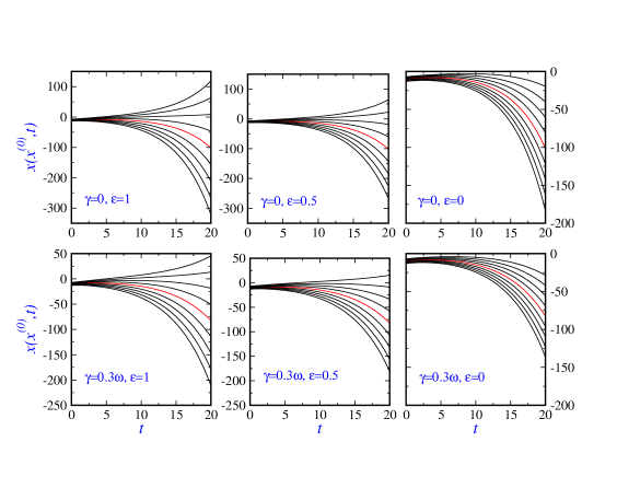
Figure 1: (Color online) Scaled trajectories issued from a propagating Gaussian wave packet under the potentail $V(x,t)=qE_{0}[\cos(\omega_{0}t+\phi)]x-\omega^{2}x^{2}/2$ in the CK approach. The red curve corresponds to the classical motion of the center of the wave packet. In each row, the friction coefficient $\gamma$ is constant: $\gamma=0$ (first row) and $\gamma=0.3\omega$ (second row). In each column, the dynamical regime given by $\epsilon$ is constant: quantum regime, $\epsilon=1$ (first column); intermediate regime, $\epsilon=0.5$ (second column); and classical regime, $\epsilon=0$ (third column). Parameters have been fixed as follows: $\phi=0$, $\omega_{0}=\omega=0.2$, $E_{0}=0.1$, $x_{0}=-10$, $\sigma_{0}=1$ and $p_{0}=1$.

In Figure 1, scaled trajectories are plotted in the CK framework for different dynamical regimes ruled by $\epsilon$ for the non-dissipative, $\gamma=0$ (top panels), and dissipative, $\gamma=0.3\omega$ (bottom panels), cases. The field parameters are $E_{0}=0.1$, $\omega_{0}=\omega=0.2$ and $\phi=0$. A uniform distribution of initial positions in the range $[x_{0}-3\sigma_{0},x_{0}+3\sigma_{0}]$ for the initial Gaussian probability density function $\tilde{\rho}(x,0)$ is used. In each plot, the red curve corresponds to the motion of center of the wave packet which is a classical path independent on $\epsilon$. Three different regimes are then identified: classical regime, $\epsilon=0$, intermediate or transition regime, $\epsilon=0.5$, and quantum regime with $\epsilon=1$.

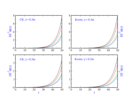
Figure 2: Width of the wave packet versus time in the CK (first column) and Kostin (second column) approaches for different values of the dynamical regime: $\epsilon=1$ (black), $\epsilon=0.5$ (red), $\epsilon=0.1$ (green) and $\epsilon=0$ (blue) and two values of friction: $\gamma=0.3\omega$ (first row) and $\gamma=0.5\omega$ (second row). Values of the field parameters are the same as in Figure 1.

As expected, classical trajectories (for $\epsilon=0$) do not cross the barrier revealing the characteristics of tunnelling process. However, in the transition to quantum regime, some particles pass the barrier. In particular, some of them above the red curve which their initial positions are located in the right tail of the initial Gaussian wave packet. These plots clearly reveal that the tunnelling process is present. Scaled trajectories coming from the Kostin approach have the same behavior.

The time evolution of the wave packet width $\tilde{\sigma}(t)$ is shown in Fig.2 for different values of the dynamical regime: $\epsilon=1$ (black curve), $\epsilon=0.5$ (red curve), $\epsilon=0.1$ (green curve) and $\epsilon=0$ (blue curve) in the CK approach (first column) and the Kostin approach (second column). Two values of dissipation $\gamma=0.3\omega$ (first row) and $\gamma=0.5\omega$ (second row) are chosen. In both cases, the widths increase with time but always we have that $\sigma_{\text{CK}}(t)<\sigma_{\text{Kostin}}(t)$ indicating that tunnelling is more important in the Kostin framework. When passing from the quantum to classical regime, the corresponding widths decrease smoothly leading to a reduction of the weight of the wave part of the scaled trajectories in the dressing scheme and, therefore, to the increase of the decoherence. This fact is reinforced with dissipation since the spread of the probability density diminishes showing a tendency to observe localization.

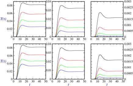
Figure 3: (Color online) Transmission probability as a function of time, $T(t)$, for different values of dissipation: $\gamma=0$ (black curve), $\gamma=0.1\omega$ (red curve), $\gamma=0.2\omega$ (green curve) and $\gamma=0.3\omega$ (blue curve). This probability is also plotted for $\epsilon=1$ (first column), $\epsilon=0.5$ (second column) and $\epsilon=0.1$ (third column) in the CK (first row) and Kostin (second row) approaches. Values of the field parameters are the same than in figure 1.

Transmission probability is displayed versus time in Figure 3. Four different values of dissipation are chosen: $\gamma=0$ (black curve), $\gamma=0.1\omega$ (red curve), $\gamma=0.2\omega$ (green curve) and $\gamma=0.3\omega$ (blue curve). This probability is also plotted for different dynamical regimes $\epsilon=1$ (first column), $\epsilon=0.5$ (second column) and $\epsilon=0.1$ (third column) in the CK (first row) and Kostin (second row) frameworks. Several interesting features are noticed. First, with friction, the transmission probabilities strongly decrease in both cases. Second, with the transition parameter $\epsilon$, this probability also decreases when passing from the quantum regime to a nearly classical regime ($\epsilon=0.1$). And, finally, the Kostin approach always displays a higher tunnelling process than the CK one. According to Eq. (62), the transmission probability is determined by ${\text{erf}}(x_{t}/\sqrt{2}\tilde{\sigma}(t))$. Since the error function is an increasing function of its argument and $x_{t}$ is negative for tunnelling (see Fig. 1), then from $\tilde{\sigma}_{\text{CK}}(t)<\tilde{\sigma}_{\text{Kostin}}(t)$, one sees that this probability is higher in the Kostin approach. This is also well illustrated in Fig. 4 where transmission probabilities are plotted as a function of the transition parameter at different dissipative values for the two cases. These probabilities are evaluated at $t=150$ where a constant value of $T$ is already reached. As expected, these probabilities decrease with $\epsilon$ and $\gamma$ where the decoherence process is playing a major role.

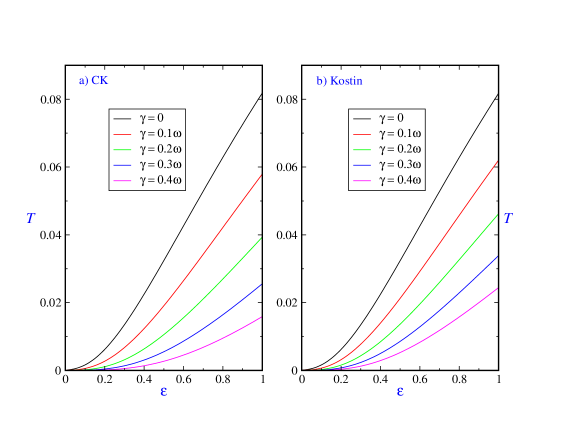
Figure 4: (Color online) Transmission probability versus transition parameter $\epsilon$ for different values of $\gamma$ within a) the CK and b) Kostin framework. Values of the field parameters are the same as in Figure 1.

Moreover, for our choice of parameters, and according to Fig. 3 the transmission probability becomes constant after $t\approx 30$ and displays a maximum at very short times. This maximum corresponds to trajectories passing through the barrier but after a while turn around. A selection of such trajectories are shown in Figure 5 for the non-dissipative motion in the quantum regime.

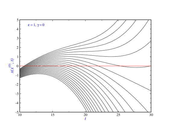
Figure 5: (Color online) A selection of scaled, $\epsilon=1$ (quantum), trajectories for the non-dissipative motion. The top of the parabolic barrier is shown by the red line. Values of the field parameters are the same as in figure 1.

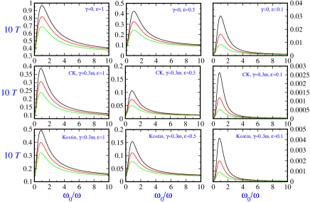
Figure 6: (Color online) Transmission probability versus the frequency (in units of $\omega$) of the applied field for different amplitudes: $E_{0}=0.12$ (black curve), $E_{0}=0.1$ (red curve) and $E_{0}=0.08$ (green curve). The remianing parameters are the same as in figure 1 but with $\phi=-\pi/2$. For easy comparison, in the first, second and third rows, the nondissipative motion, the CK and Kostin approach (for $\gamma=0.3\omega$) are considered, repectively. The different dynamical regimes are shown in the three columns with $\epsilon=1$, $\epsilon=0.5$ and $\epsilon=0.1$.

Let us analyze now the effect of the oscillatory field in this dissipative tunnelling dynamics. As has been shown before, the width $\tilde{\sigma}(t)$ of the wave packet does not depend on the field parameters. Therefore, the variation of the tunnelling probability with the field parameters comes solely through $x_{t}$. Figures 6, 7 and 8 display the dependence of transmission probability to the field parameters $\omega_{0}$, $E_{0}$ and $\phi$. In all of these figures, the transmission probability is always higher in the Kostin approach at the same friction parameter. Figure 6 shows the transmission probabilities versus the frequency (in units of $\omega$) of the applied field for different amplitudes: $E_{0}=0.12$ (black curve), $E_{0}=0.1$ (red curve) and $E_{0}=0.08$ (green curve) with $\phi=-\pi/2$. With this initial phase, the field is a pure sine function of $(\omega_{0}t)$. For easy comparison, in the first, second and third rows, the nondissipative motion, the CK and Kostin approach (for $\gamma=0.3\omega$) are considered, repectively. The different dynamical regimes are also shown in the three columns with $\epsilon=1$, $\epsilon=0.5$ and $\epsilon=0.1$. The initial values of the Gaussian wave packet are the same as in Fig. 1. A gradual decreasing of tunnelling is seen with $\epsilon$, that is, when approaching the classical regime. In the absence of the field which this occurs when $\omega_{0}=0$, the transmission probability is different from zero in the nonclassical regime. A maximum is again observed in all cases but this time is not due to the back recrossing of the scaled trajectories. This maximum is now attributed to a resonant transmission. As expected, in the absence of friction, the resonance takes place when $\omega_{0}=\omega$. On the contrary, for a viscous medium, this resonant mechanism is observed for $\omega_{0}<\omega$. In our case, $\omega_{0,\text{res}}\approx 0.86\omega$. Furthermore, the role of the field amplitude is just the reverse of the friction, when increasing its value, the corresponding probabilities also increase in a nonlinear way. In the near classical regime $\epsilon=0.1$, the tunnelling is very small. All of these features are better illustrated in Fig. 7 where transmission probabilities are plotted versus the amplitude of the applied field for different values of the frequency: $\omega_{0}=0.5\omega$ (black curve), $\omega_{0}=\omega_{0,\text{res}}\approx 0.86\omega$ (red curve) and $\omega_{0}=3\omega$ (green curve) at different dynamical regimes in the two approaches with $\gamma=0.3\omega$. The resonance or red curve gives the maximum value of the transmission probability.

The behaviour of the tunnelling process as a function of the initial phase of the applied field is plotted in Fig. 8. Transmission probabilities versus $\phi$ for different dynamical regimes $\epsilon=1$(black curve), $\epsilon=0.7$(red curve), $\epsilon=0.5$(green curve), $\epsilon=0.3$(blue curve) and $\epsilon=0.1$(magenta curve) for the frictionless motion, and the CK and Kostin approaches with $\gamma=0.3\omega$.

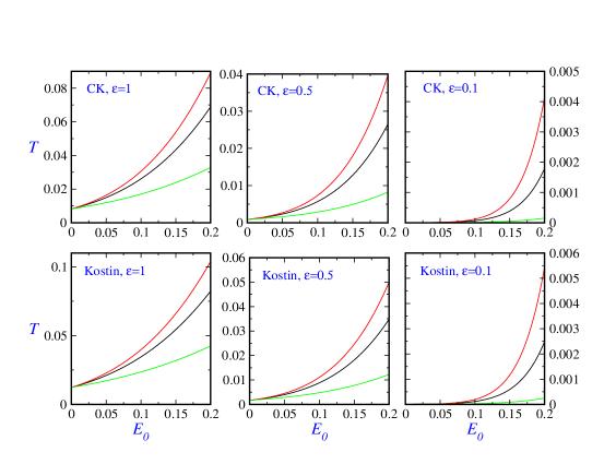
Figure 7: (Color online) Transmission probability versus the amplitude of the applied field for different values of the frequency: $\omega_{0}=0.5\omega$ (black curve), $\omega_{0}=\omega_{0,\text{res}}\approx 0.86\omega$ (red curve) and $\omega_{0}=3\omega$ (green curve) at different dynamical regimes in the two approaches with $\gamma=0.3\omega$. The remaining parameters are the same as figure 1 apart from $\phi=-\pi/2$.

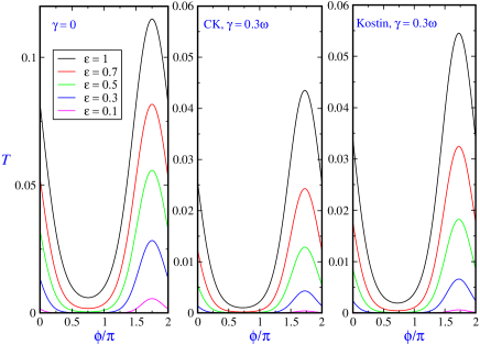
Figure 8: (Color online) Transmission probability versus the phase of the applied filed, $\phi$, for different dynamical regimes $\epsilon=1$(black curve), $\epsilon=0.7$(red curve), $\epsilon=0.5$(green curve), $\epsilon=0.3$(blue curve) and $\epsilon=0.1$(magenta curve) with $\gamma=0.3\omega$. Other parameters are the same as those of figure 1.

In this figure, a resonant behaviour is again seen for all the dynamical regimes. The maximum corresponds to $\phi\approx 1.75\pi$ with $\omega_{0}=0.2$.

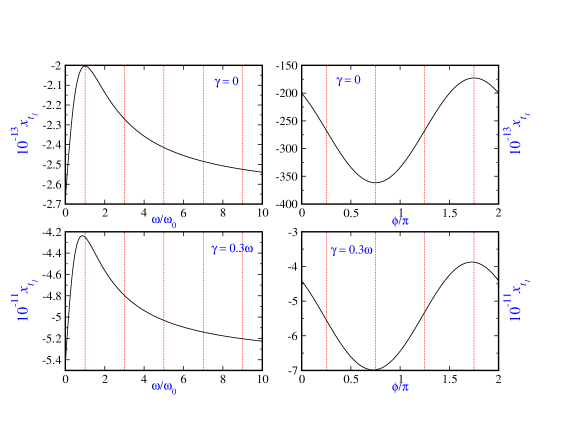
Figure 9: (Color online) Position of the wave packet center at time $t_{1}=150$ in which the transmission probability is computed versus the frequency $\omega_{0}$ (left column) and phase $\phi$ (right column) field. The remaining parameters are the same as those of figure 1. Grid lines are included for better inspection. In the frictionless motion, the maxima of $x_{t_{1}}$ versus $\omega_{0}$ and $\phi$ are located at $\omega_{0}=\omega$ and $\phi=1.75\pi$, respectively. For $\gamma=0.3\omega$, the maxima are located at values $\omega_{0}=0.86\omega$ and $\phi\approx 1.73\pi$, respectively. $x_{t_{1}}$ becomes minimum for $\phi=0.75\pi$.

As commented above, the transmission probability depends on the field parameters only through the classical trajectory $x_{t}$. In order to understand the location of the resonance of this probability versus $\omega_{0}$ and $\phi$, a close inspection to $x_{t}$ should be carried out. To this end, in Fig. 9, the center of the wave packet is plotted at $t_{1}=150$ versus $\omega_{0}$ and $\phi$ separately. In the frictionless motion, the maxima of $x_{t_{1}}$ versus $\omega_{0}$ and $\phi$ are located at $\omega_{0}=\omega$ and $\phi=1.75\pi$, respectively. On the contrary, for $\gamma=0.3\omega$, the maxima are located at values $\omega_{0}=0.86\omega$ and $\phi\approx 1.73\pi$, respectively. It is found that $x_{t_{1}}$ becomes minimum for $\phi=0.75\pi$. Now, because of the proportionality $T\propto{\text{erf}}(x_{t_{1}}/\sqrt{2}\sigma(t_{1}))$, the maximum of $T$ coincides with the maximum of $x_{t_{1}}$. This explains the location of resonances of the transmission probabilities.

VII Conclusions

The study of dissipative tunnelling by an inverted parabolic barrier carried out here clearly shows how the decoherence process is increasing gradually with the dynamical regime considered and governed by $\epsilon$ as well as with the friction and field parameters. However, the important point is that when comparing the Kostin and CK approaches, the tunnelling probabilities are different as also observed by Tokieda and Hagino ToHa-PRC-2017 . This discrepancy comes from the differential equation governing the width of the Gaussian wave packet where both approaches differ. At this point, it is difficult to discern which approach is better suited when a comparison with experimental results is carried out. We lean towards the Kostin approach due to, at least, two points: (i) When an interaction with an environment (bath, measuring apparatus, etc) is present, linear quantum mechanics is no longer applicable and nonlinear differential equations have to be implemented for a proper description of the corresponding open quantum dynamics, and (ii) the nonlinear Kostin equation comes from the standard Langevin equation which is also issued from a Caldeira-Leggett Hamiltonian formalism, whereas the CK approach is seen more like a phenomenological or effective one. In any case, new theoretical developments and numerical simulations are necessary to be implemented and compared with existing experimental results in order to have a better description of this open dynamics. A natural extension of this work is to include the stochasticity into the dynamics through a random force or noise term.

Acknowledgements SVM acknowledges partial support from the University of Qom and SMA support from the Ministerio de Economía y Competitividad (Spain) under the Project FIS2014-52172-C2-1-P.

References

- (1) U. Weiss, Quantum Dissipative Systems, World Scientific, Singapore, 1999.
- (2) M. Razavy, Classical and Quantum Dissipative Systems, Imperial College Press, London, 2005.
- (3) A. B. Nassar and S. Miret-Artés, Bohmian Mechanics, Open Quantum Systems and Continuous Measurements (Springer, 2017).
- (4) S. Baskoutas and A. Jannussis, J. Phys. A: Math. Gen. 25 (1992) L1299.
- (5) G. J. Papadopoulos, J. Phys. A: Math. Gen. 30 (1997) 5497.
- (6) M. D. Kostin, J. Chem. Phys. 57 (1972) 3589.
- (7) P. Caldirola, Nuovo Cimento 18 (1941) 393-400.
- (8) E. Kanai, Prog. Theor. Phys. 3 (1948) 440-442.
- (9) A: S. Sanz, R. Martinez-Casado, H. C. Peñate-Rodriguez, G. Rojas-Lorenzo, S. Miret-Artés, Ann. Phys. 347 (2014) 1-20.
- (10) S. V. Mousavi and S. Miret-Artés, J. Phys. Commun. 2 (2018) 035029
- (11) P. R. Holland, The Quantum Theory of Motion (Cambridge University Press, 1993).
- (12) A. S. Sanz, S. Miret-Artés, A Trajectory Description of Quantum Processes. Part I. Fundamentals. Lecture Notes in Physics, Vol. 850, 2012.
- (13) A. S. Sanz, S. Miret-Artés, A Trajectory Description of Quantum Processes. Part II. Applications. Lecture Notes in Physics, Vol. 831, 2014.
- (14) M. Tokieda and K. Hagino, Phys. Rev. C 95 (2017) 054604.
- (15) C. D. Richardson, P. Schlagheck, J. Martin, N. Vandewalle, and T. Bastin, Phys. Rev. A 89 (2014) 032118.
- (16) C.-C. Chou, Ann. Phys. 371 (2016) 437.
- (17) C.-C. Chou, Int. J. Quan. Chem. 116 (2016) 1752.
- (18) D. Home, A. K. Pan and A. Banerjee, J. Phys. A: Math. Theor. 42 (2009) 165302.
- (19) R. Schiller, Phys. Rev. 125 (1962) 1100.
- (20) C. Zander, A. R. Plastino, J. Díaz-Alonso, Ann. Phys. 362 (2015) 36.
- (21) C. R. Leavens in Time in Quantum Mechanics, Edited by J. G. Muga, R. Sala and I. L. Egusquiza, Springer, Berlin, 2002.
- (22) G. J. Papadopoulos, J. Phys. A: Math. Gen. 23 (1990) 935.
- (23) I. S. Gradshteyn and I. M. Ryzhik, Table of Integrals, Series and Products (Academic Press, Inc., 1980.)