Finite element model updating for structural applications

Finite element model updating for structural applications

Abstract

A novel method for performing model updating on finite element models is presented. The approach is particularly tailored to modal analyses of buildings, by which the lowest frequencies, obtained by using sensors and system identification approaches, need to be matched to the numerical ones predicted by the model. This is done by optimizing some unknown material parameters (such as mass density and Young’s modulus) of the materials and/or the boundary conditions, which are often known only approximately. In particular, this is the case when considering historical buildings.

The straightforward application of a general-purpose optimizer can be impractical, given the large size of the model involved. In the paper, we show that, by slightly modifying the projection scheme used to compute the eigenvalues at the lowest end of the spectrum one can obtain local parametric reduced order models that, embedded in a trust-region scheme, form the basis for a reliable and efficient specialized algorithm.

We describe an optimization strategy based on this approach, and we provide numerical experiments that confirm its effectiveness and accuracy.

1 Introduction

Finite element (FE) model updating is a procedure aimed at calibrating the FE model of a structure in order to match numerical and experimental results. Introduced in the 1980s, it turned out to play a crucial role in the design, analysis and maintenance of aerospace, mechanical and civil engineering structures [14, 19, 23, 29]. In structural mechanics, model updating techniques are used in conjunction with vibrations measurements to determine unknown system characteristics, such as the materials’ properties, constraints, etc. The resulting updated FE model can then be used to obtain reliable predictions on the dynamic behavior of the structure subjected to time-dependent loads. A further important application of model updating, within the framework of structural health monitoring, is damage detection [39, 42]. Within this framework, damage can be identified based on the assumption that its presence is associated with a decrease in the stiffness of some elements, with consequent changes to the structure’s modal characteristics.

Finite element model updating involves the solution of a constrained optimization problem, whose objective function is generally expressed as the discrepancy between experimental and numerical quantities, such as the structure’s natural frequencies and mode shapes. The constraints are given by the boundary conditions and other physical limitations to the degrees of freedom involved. Ill-posedness or ill-conditioning can affect model updating formulations and lead to numerical problems due to inaccuracy in the model and lack of information in the measurements. Among the methods aimed at quantifying uncertainties, the probabilistic Bayesian approach is one of the most adopted [39].

Application of FE model updating to ancient masonry buildings is relatively recent. In [4, 5, 12, 13, 15, 20, 22, 24, 27, 33, 37, 38, 43] a vibration-based model updating is conducted, and preliminary FE models are tuned by using the dynamic characteristics determined through system identification techniques. In the papers cited above the modal analysis of the FE models are conducted via commercial codes, and the model updating procedure is implemented separately. In this paper, on the contrary, FE model updating is integrated within a software package, the NOSA-ITACA code [11], able to manage the large-scale problems encountered in applications. In particular, the algorithms for the solution of the constrained optimization problem integrated in NOSA-ITACA exploit the structure of the stiffness and mass matrices and the fact that only a few of the smallest eigenvalues have to be calculated. This new procedure reduces both the total computation time of the numerical process and user’s effort, thus providing the scientific and technical communities with efficient algorithms specific for FE model updating.

A simple form of FE model updating has been employed in combination with the NOSA-ITACA code in [6, 7, 32], to perform modal analyses of the San Frediano bell tower and the Clock tower in Lucca, Italy. In these works the optimal values of Young’s modulus and the materials’ mass density are determined by fitting the data measured by seismometric stations placed on the towers and running several simulation on a grid of feasible values. However, this approach becomes impractical if the number of free parameters or the size of the model is considerably increased.

Model reduction techniques have long been used to reduce the size of complex FE models to a more manageable order. This allows, for example, performing more demanding, and computationally costly, numerical tasks, such as optimization, simulation, and so on, in an efficient manner. In particular, reduced models are natural candidates for optimization of the model’s free parameters, either to improve some engineering properties or to better match the empirically measured modes. In practice, this step often turns into an eigenvalue optimization, where part of the spectral structure is tuned following some prescribed criteria.

However, when the model depends on parameters, it is generally non-trivial to obtain a reduced parametric model that accurately reflects the behavior of the original one for all possible parameter values. This is precisely the aim of so-called parametric model reduction, which has recently been used in combination with optimization algorithms [3, 30, 36, 45], especially involving trust-region solvers [1, 44]. In this work, we propose an efficient model reduction strategy derived by properly recycling the Lanczos projection. Our approach is tailored to the needs of structural FE analysis.

In fact, FE study of buildings has some peculiar features that justify trying to devise an adapted method. As discussed in the following, in this context the natural frequencies of interest are those at the lowest end of the real spectrum. In order to compute them accurately, the natural choice is an (inverse) Lanczos method. When a parametric model is given, the Lanczos projection can be re-interpreted as a parameter dependent model reduction, whereby only the relevant part of the spectrum is matched. We show that this step can be performed efficiently, and that its combination with a trust-region method allows matching the measured frequencies with the ones predicted by the parametric model.

The paper is organized as follows. In Section 2 we briefly discuss the FE model for the structural applications we are interested in, and formulate the optimization problem related to model updating. In Section 3 we recall the requirement for a model to be used in a trust-region optimization method, in particular those required to guarantee convergence. Section 4 describes how to construct a model that satisfies these requirements by slightly modifying the Lanczos projection step used to compute the smallest frequencies, and finally Section 5 illustrates some tests of our implementation on some problems. In Section 6 we draw some conclusions and discuss future lines of research.

2 The model: modal analysis of masonry buildings and frequency matching

Although the constituent masonry materials of historical buildings exhibit different strengths under tension and compression and, therefore, behave nonlinearly, modal analysis, which is based on the assumption that the materials are linear elastic, is widely used in applications and provides important qualitative information on the dynamic behavior of masonry structures. Modal analysis consists in the solution of the constrained generalized eigenvalue problem

$$K\,v =\omega^{2}\,M\,v, \text{subject to }\ \ Cv =0,$$ (1)

with $C\in\mathbb{R}^{h\times n}$ and $h\ll n$. The left part of (1) is derived from the differential equation

$$M\ddot{u}+Ku=0,$$ (2)

governing the undamped free vibrations of a linear elastic structure discretized into finite elements. In (2) $u$ is the displacement vector, which belongs to $\mathbb{R}^{n}$ and depends on time $t$, $\ddot{u}$ is the second-derivative of $u$ with respect to $t$, and $K$ and $M\in\mathbb{R}^{n\times n}$ are the stiffness and mass matrices of the FE model. $K$ is symmetric and positive-semidefinite, $M$ is symmetric and positive-definite, and both are sparse and banded. Displacements $u_{i}$ are also called degrees of freedom; the integer $n$ is the total number of degrees of freedom of the system and is generally very large, since it depends on the level of discretization of the problem. By assuming that

$$u=v\cdot\sin(\omega t),$$ (3)

with $v$ a vector of $\mathbb{R}^{n}$ and $\omega$ a real scalar, and applying the mode superposition procedure [9], equation (2) is transformed into the generalized eigenvalue problem (1). The right part of equation (1) expresses the fixed constraints and the master-slave relations assigned to displacement $u$, written in terms of vector $v$. Imposing the constraints and boundary conditions is equivalent to projecting the matrices $K$ and $M$ on a subspace where they are a symmetric positive definite pencil (the right kernel of the operator $C$). In the following, we assume that this projection has already been done — and we refer the reader to [35] for further details. Notice, in particular, that if $K$ and $M$ depend linearly on some parameters $\mathbf{x}:=(x_{1},\ldots,x_{\ell})$, the same holds true for their projection. More generally, the smooth dependency of $K$ and $M$ is preserved by the projection, since it is a linear operation. This will be exploited in the analysis of the parametric projection in Section 4.

The eigenvalues $\omega_{i}^{2}$ of (1) are linked to the natural frequencies, or eigenfrequencies $f_{i}$ of the structure via the relation $f_{i}=\omega_{i}/2\pi$, and the eigenvectors $v^{(i)}$ are the corresponding mode shape vectors, or eigenmodes. Together with the natural frequencies, the mode shapes provide a good deal of qualitative information on the structure’s deformations under dynamic loads.

Measuring the vibrations of masonry buildings is a common practice for assessing their dynamic behavior. Historic constructions are subjected to a number sources of vibrations, such as traffic, micro–tremors, wind and earthquakes. The availability of sensitive instruments to detect buildings’ movements makes it possible to conduct accurate, long–term monitoring campaigns. In fact, ambient vibration monitoring can provide important information on the structural health of old masonry constructions, as it is a non-destructive technique able to capture the most important features of their dynamic behavior, such as natural frequencies, damping ratios, mode shapes and wave propagation velocities. Once the influence of environmental factors has been accounted for, changes in these dynamic properties over time may represent effective structural damage indicators [7].

FE model updating is a procedure that enables calibrating a finite element model of a structure in order to match numerical and experimental results. Thus, model updating techniques are used in conjunction with vibrations measurements to determine a structure’s characteristic, such as materials’ properties, constraints, etc., which are generally unknown.

2.1 Formulation of the optimization problem

The model updating problem can be reformulated as an optimization problem by assuming that the (projected) stiffness and mass matrices $K$ and $M$ are functions of the parameter vectors $\mathbf{x}$. We use the notation

$$K:=K(\mathbf{x}),\qquad M:=M(\mathbf{x}),\qquad\mathbf{x}\in\mathbb{R}^{\ell},$$

to denote this dependency. The set of valid choices for the parameters is denoted by $\Omega$, which we assume to be an $\ell$-dimensional box, that is

$$\Omega=[a_{1},b_{1}]\times\ldots\times[a_{\ell},b_{\ell}],$$ (4)

for certain values $a_{i}<b_{i}$, $i=1,\ldots,\ell$. We also assume that initial estimates for the parameter values are available, and we denote these by $\mathbf{x}^{(0)}$. When this is not the case, we choose $\mathbf{x}^{(0)}$ as the center of the box $\Omega$ (i.e., the vector with the midpoints of the intervals $[a_{i},b_{i}]$ as coordinates).

Our ultimate aim is to determine the optimal value of $\mathbf{x}$ that minimizes a certain cost functional $\phi(\mathbf{x})$ within the box $\Omega$. This is an instance of the optimization problem

$$\min_{\mathbf{x}\in\Omega}\phi(\mathbf{x}).$$ (5)

The choice of the objective function $\phi(\mathbf{x})$ is related to the frequencies that we want to match. If we need to match $s$ frequencies of the model, we choose a suitable weight vector $\mathbf{w}:=[w_{1},\ldots,w_{s}]$, with $w_{i}\geqslant 0$, and define the functional $\phi(\mathbf{x})$ as follows:

$$\phi(\mathbf{x}):=\left\lVert\frac{\sqrt{\Lambda_{s}(K,M)}}{2\pi}-\mathbf{f}\right\rVert_{\mathbf{w},2}^{2},\qquad\lVert\mathbf{y}\rVert_{\mathbf{w},2}:=\sqrt{\mathbf{y}^{T}D_{\mathbf{w}}^{2}\mathbf{y}},$$ (6)

where $\mathbf{f}$ is the vector of the measured frequencies, $D_{\mathbf{w}}=\mathrm{diag}(w_{1},\ldots,w_{s})$ and $\Lambda_{s}(K,M)$ is the vector containing the smallest $s$ eigenvalues of the pencil $K-\lambda M$, ordered according to their magnitude.

The vector $\mathbf{w}$ encodes the weights that should be given to each frequency in the optimization scheme. If the aim is to minimize the distance between the vector of measured and computed frequencies in the usual Euclidean norm, then $\mathbf{w}=\mathbbm{1}_{s}$, the vector of all ones, should be chosen. If, instead, a relative accuracy on the frequencies is desired, $w_{i}=f_{i}^{-1}$ is the natural choice. To avoid scaling issues in the objective function, we always normalize $\mathbf{w}$ to have Euclidean norm $1$.

3 The optimization framework

In this section we describe the optimization framework that we use. We choose to rely on a trust-region scheme, which is defined by building a sequence of local models for the objective function.

Construction of the local models is discussed in Section 4, where we show that such models satisfy the minimal requirements for a well-defined trust-region scheme. The practical choice of the objective function and the weights has been deferred to Section 5, where several options are discussed.

3.1 Trust region methods

Trust-region methods are well-known iterative methods for solving bound-constrained optimization problems, see e.g. [16, 17, 34]. Their main distinctive features are robustness and convergence to first-order critical points regardless of the choice of the initial estimate.

We now review the basic steps in a trust-region algorithm for solving the bound-constrained optimization problem of Equation (5), where $\phi:\mathbb{R}^{\ell}\rightarrow\mathbb{R}$ is a smooth function and $\Omega$ is defined as in (4).

The key idea of a trust-region method is to define, at iteration $k$, a model $\phi^{\cal R}_{k}$ for the objective function $\phi$ around the current iterate $\mathbf{x}^{(k)}$, together with a region within such model can be trusted to provide an adequate representation of $\phi$. The trial step $\mathbf{s}^{(k)}$ is then computed, either exactly or approximately, by minimizing this model within the trust-region. The trust-region is the set of all points

$${\mathcal{B}}_{k}=\{\mathbf{x}\in\mathbb{R}^{\ell}|\,\|\mathbf{x}-\mathbf{x}^{(k)}\|\leqslant\Delta_{k}\},$$

where $\Delta_{k}$ is called the trust-region radius and $\|\cdot\|$ is a norm equivalent to the Euclidean norm.

Due to the presence of bound-constraints, all the generated iterates $\mathbf{x}^{(k)}$ must be ensured to be feasible, that is, $\mathbf{x}^{(k)}\in\Omega$ for all $k\geqslant 0$. One strategy consists in minimizing the model within the set $\mathcal{B}_{k}\cap\Omega$. When the feasible set $\Omega$ is a box, the trust-region is generally defined using the $\infty$ norm.

Having minimized the model on $\mathcal{B}_{k}\cap\Omega$, it must be decided whether to accept the trial step or to change the trust-region radius. Usually, the trust-region radius and the new point $\mathbf{x}^{(k)}+\mathbf{s}^{(k)}$ are tested simultaneously to assess the quality of the approximation yielded by the local model. This is measured using the ratio $\rho^{(k)}$ between the actual and the predicted reduction defined as follows:

$$\rho^{(k)}=\frac{\phi(\mathbf{x}^{(k)})-\phi(\mathbf{x}^{(k)}+\mathbf{s}^{(k)})}{\phi^{\cal R}_{k}(\mathbf{x}^{(k)})-\phi^{\cal R}_{k}(\mathbf{x}^{(k)}+\mathbf{s}^{(k)})}$$ (7)

If $\rho^{(k)}$ is close to 1, there is good agreement between the model $\phi^{\cal R}$ and the function $\phi$ over this step, so $\mathbf{x}^{(k)}+\mathbf{s}^{(k)}$ is accepted as the new iterate and it is safe to increase the radius of the trust-region for the next iteration. If $\rho^{(k)}$ is positive but not close to 1, then $\mathbf{x}^{(k+1)}=\mathbf{x}^{(k)}+\mathbf{s}^{(k)}$ but the trust-region radius is not altered. If $\rho^{(k)}$ is close to zero or negative, step $\mathbf{s}^{(k)}$ is rejected and the trust-region radius is shrunk.

Convergence of the iterative process is declared when a suitable criticality measure is sufficiently small. We consider the measure

$$\chi(\mathbf{x}^{(k)})=\|P_{\Omega}(\mathbf{x}^{(k)}-\nabla\phi(\mathbf{x}^{(k)}))-\mathbf{x}^{(k)})\|$$ (8)

where $P_{\Omega}$ is the projection onto the feasible set, and $\chi(\mathbf{x}^{(k)})$ is the norm of the projected gradient onto the box, and reduces to $\lVert\nabla\phi(\mathbf{x}^{(k)})\rVert$ when $\mathbf{x}^{(k)}$ is in the interior of $\Omega$. The approach is summarized in the pseudocode of Algorithm 1 where we assume that the model functions are minimized “exactly” (as it will be the case in our applications, see Section 5.1).

The initial point $\mathbf{x}^{(0)}\in\Omega$, an initial trust-region radius $\Delta_{0}$, the constants $\eta_{1},\eta_{2},\gamma_{1},\gamma_{2}$ such that

$$0<\eta_{1}\leqslant\eta_{2}<1\mbox{ and }0<\gamma_{1}\leqslant\gamma_{2}<1,$$

$k_{max}>0$ and $\epsilon>0$.

Compute $\phi(\mathbf{x}^{(0)})$

for $k=1,\ldots,k_{max}$ do

     Define a model $\phi^{\cal R}_{k}$ in $\mathcal{B}_{k}\cap\Omega$.

     Compute a step $\mathbf{s}^{(k)}$ that minimizes the model and such that $\mathbf{x}^{(k)}+\mathbf{s}^{(k)}\in\mathcal{B}_{k}\cap\Omega$.

     Compute $\phi(\mathbf{x}^{(k)}+\mathbf{s}^{(k)})$ and define the ratio (7).

     if $\rho^{(k)}\geqslant 1$ then

         define $\mathbf{x}^{(k+1)}=\mathbf{x}^{(k)}+\mathbf{s}^{(k)}$;

     else

         define $\mathbf{x}^{(k+1)}=\mathbf{x}^{(k)}$.

     end if

     Update the trust-region radius setting

$$\Delta_{k+1}\in\left\{\begin{array}[]{ll}\left[\Delta_{k},\infty\right)&\mbox{ if }\rho^{(k)}\geqslant\eta_{2}\\ \left[\gamma_{2}\Delta_{k},\Delta_{k}\right]&\mbox{ if }\rho^{(k)}\in[\eta_{1},\eta_{2})\\ \left[\gamma_{1}\Delta_{k},\gamma_{2}\Delta_{k}\right]&\mbox{ if }\rho^{(k)}<\eta_{1}\end{array}\right.$$

     Compute the criticality measure (8).

     if  $\chi(\mathbf{x}^{(k+1)})\leqslant\epsilon$ then

         return An approximate first-order critical point $\mathbf{x}^{(k+1)}$.

     end if

end for

Algorithm 1 Basic trust-region algorithm

In order to obtain a robust and globally convergent trust-region algorithm involving approximate models, the following assumptions should hold [17] for the objective $\phi$ and the model $\phi^{\cal R}_{k}$ functions:

(AF.1) $\phi:\mathbb{R}^{\ell}\rightarrow\mathbb{R}$ is twice-continuously differentiable on $\Omega$.

(AF.2) The function $\phi$ is bounded below for all $\mathbf{x}\in\Omega$.

(AF.3) The second derivatives of $\phi$ are uniformly bounded for all $\mathbf{x}\in\Omega$.

(AM.1) For all $k$, $\phi^{\cal R}_{k}$ is twice differentiable on ${\mathcal{B}}_{k}$.

(AM.2) The values of the objective and the model function coincide at the current iterate, i.e., for all $k$,

$$\phi(\mathbf{x}^{(k)})=\phi^{\cal R}_{k}(\mathbf{x}^{(k)}).$$

(AM.3) The gradients of the objective and the model function coincide at the current iterate, i.e., for all $k$,

$$\nabla\phi(\mathbf{x}^{(k)})=\nabla\phi^{\cal R}_{k}(\mathbf{x}^{(k)}).$$

(AM.4) The second derivatives of $\phi^{\cal R}(\mathbf{x}^{(k)})$ remain bounded within the trust-region ${\mathcal{B}}_{k}$ for all $k$.

Theorem 3.1.

[17, Section 12.2.2] Under Assumptions (AF.1)-(AF.3) and (AM.1)-(AM.4), every limit point of the sequence $\{\mathbf{x}^{(k)}\}$ generated by Algorithm 1 is first-order critical, i.e.

$$\lim_{k\rightarrow\infty}\|P_{\Omega}(\mathbf{x}^{(k)}-\nabla\phi(\mathbf{x}^{(k)}))-\mathbf{x}^{(k)})\|=0.$$

3.2 Enforcing first-order matching

Here we use the trust-region framework described in the previous section to solve problem (5) with objective function (6). Note that conditions (AF.1) – (AF.3) are automatically satisfied by our definition of objective function. As discussed in Section 4.1, the local model $\widetilde{\phi}_{k}^{\mathcal{R}}(\mathbf{x})$ that we build does not necessarily agree at the first order with the original function $\phi(\mathbf{x})$, which apparently breaks assumption (AM.3) — and only satisfies (AM.2). However, if the gradient $\nabla\phi_{k}^{\cal R}(\mathbf{x})$ is known at the expansion point $\mathbf{x}^{(k)}$, this can be easily fixed by defining

$$\phi_{k}^{\cal R}(\mathbf{x}):=\widetilde{\phi}_{k}^{\cal R}(\mathbf{x})+(\phi(\mathbf{x}^{(k)})-\widetilde{\phi}_{k}^{\cal R}(\mathbf{x}^{(k)}))+(\nabla\phi(\mathbf{x}^{(k)})-\nabla\widetilde{\phi}_{k}^{\cal R}(\mathbf{x}^{(k)}))^{T}(\mathbf{x}-\mathbf{x}^{(k)}),$$ (9)

see, e.g., [1, 2, 25]

4 Building the reduced model by Lanczos projection

Our aim in this section is to develop a low-dimensional model of the frequencies as a function of the parameters. The model must be efficient to evaluate, and needs to satisfy the requirements for use as a local model in the trust-region approach described in Section 3.

This task can be viewed as a special case of parametric model order reduction. Several approaches have been developed in this field that allow obtaining low-dimensional models for accurately approximating the behavior of complex systems. For instance, when controlling large-scale dynamical systems, it is possible to employ projection approaches when the observations and inputs have low-rank properties (see [10] and references therein).

Our aim is slightly different; we are interested only in a particular region on the spectrum (the lowest frequencies), but we have no particular assumptions on the input (which is typically induced by the environment).

In the next sections, we first briefly summarize the standard (inverse) Lanczos iteration for matrix pencils, mainly to fix the notation, and then we show that we can perform some modifications to make it parameter dependent. We refer to [8] for a discussion of the relation between the Lanczos process and (nonparametric) model reduction.

4.1 The Lanczos method

The Lanczos iteration, for a symmetric $n\times n$ matrix $A$, can be summarized as follows. We construct an orthogonal basis $W_{m}$ for the subspace $\mathcal{K}_{m}(A,v)\subseteq\mathbb{R}^{n}$ defined as:

$$\mathcal{K}_{m}(A,v):=\mathrm{span}(v,Av,\ldots,A^{m-1}v).$$

Unless a breakdown occurs, this space has dimension $m$, and the basis $W_{m}$ is represented as a $n\times m$ orthogonal matrix (that is, $W_{m}^{T}W_{m}=I_{m}$). Given the basis, one then computes the projection $T_{m}=W_{m}^{T}AW_{m}$. The matrix $T_{m}$ is tridiagonal, and its eigenvalues (known as Ritz values) are good approximations of the extremal eigenvalues of $A$ even when $m\ll n$. This procedure is appealing for several reasons.

1. Computation of the space $W_{m}$ only requires matrix-vector multiplications, and therefore it is easy to exploit the sparsity or, more generally, the structure of $A$.

2. The orthogonalization of the basis requires only scalar products, which can be computed very efficiently if $m$ does not increase too much.

3. The algorithm can be carried out iteratively, i.e., the optimal value of $m$ does not need to be known a priori, and $T_{m}$ can be built incrementally. In our framework, we stop the iteration when the error on the computed eigenvalues is guaranteed to be smaller than a certain relative threshold $\tau$ (see [18] for a classical reference on the stopping criterion of Lanczos for computing eigenvalues). The actual value of $\tau$ is reported in Section 5.

When the matrix $A$ arises from a FE discretization of a PDE involving only local operators and elements with compact support and few overlappings, the number of nonzero elements is only $\mathcal{O}(n)$; hence, the matrix vector multiplication can be carried out with linear complexity. Moreover, the matrix usual has a band or multiband structure, and using good sparse solvers or appropriate preconditioners we can solve linear systems in $\mathcal{O}(n)$ time. Therefore, the smallest eigenvalue of $A$ can be extracted applying Lanczos to $A^{-1}$. Since we are interested in modal analysis of structures discretized by FE, we need to approximate the smallest eigenvalues of a pencil $K-\lambda M$, with $K$ and $M$ symmetric positive definite; the same technique to extract the smallest eigenvalues can be applied (implicitly) to the symmetric matrix $M^{\frac{1}{2}}K^{-1}M^{\frac{1}{2}}$, obtaining:

$$T_{m}=W_{m}^{T}M^{\frac{1}{2}}K^{-1}M^{\frac{1}{2}}W_{m}=U_{m}^{T}MK^{-1}MU_{m},\qquad U_{m}=M^{-\frac{1}{2}}W_{m}.$$

It is immediately verifiable that $U_{m}$ contains a basis of the same subspace spanned by $W_{m}$, but this matrix is $M$-orthogonal (that is, orthogonal with respect to the inner product defined by $M$), so $U_{m}^{T}MU_{m}=I_{m}$ [21].

Remark 4.1.

In the above framework, there is no need to explicitly compute the square root of the positive definite matrix $M$, which would be a very expensive operation. The matrix $T_{m}$ is implicitly obtained using the matrix-vector product with $MK^{-1}M$ and re-orthogonalization by the scalar-product induced by $M$, computing the basis $U_{m}$ directly.

However, using this procedure as a black-box to evaluate the objective function in an optimization method can easily become too onerous: even if the complexity is only linear, the size of the problem can make this operation unpractical (we often deal with $n\approx 10^{6}$ or even more in finite element models).

Therefore, we wish to investigate the use of the Lanczos process to build a local parametric reduced model for the case when $K$ and $M$ are not constant matrices, but depend on $\ell$ parameters $x_{1},\ldots,x_{\ell}$.

4.2 Parametric finite element models

Let us assume that a finite element model depending on a variable $\mathbf{x}\in\mathbb{R}^{\ell}$ is given. These parameters $\mathbf{x}$ may encode different properties of the system (our method does not make any assumption about what they mean — but only on their algebraic properties). Most of the time, these will be some materials’ physical characteristics, such as Young’s modulus, or mass density. In almost all the cases of interest, the dependency is linear in $\mathbf{x}$. However, for our discussion we just assume it to be smooth, i.e., at least $\mathcal{C}^{2}$.

4.3 A first-order approximation to the updated Lanczos projection

In this section we develop a strategy that, given a certain initial value $\mathbf{x}^{(0)}$ for the model parameters, builds a local model to be used in the trust-region scheme presented in Section 3.

Let us denote with $F(\mathbf{x})$ the matrix valued function that, for a given choice of the parameters $\mathbf{x}$, returns the tridiagonal matrix obtained running the Lanczos process on $M^{\frac{1}{2}}(\mathbf{x})K(\mathbf{x})^{-1}M^{\frac{1}{2}}(\mathbf{x})$.

We shall approximate $F(\mathbf{x})$ in a neighborhood of $\mathbf{x}^{(0)}$. This approximation calls for two steps: first, we fix the subspace used for the projection, as described in Lemma 4.3, obtaining an approximation $F_{0}(\mathbf{x})$ of $F(\mathbf{x})$. Then, we show how to further approximate this function in order to make it cheap to evaluate. Lemma 4.7 describes how to combine these approximations to obtain a first-order correct local model for the trust-region scheme.

Remark 4.2.

The outcome of the Lanczos process depends on the initial vector chosen for the scheme. Here and in the following, we assume that this vector is fixed whenever we keep $\mathbf{x}^{(0)}$ unchanged. This makes the subspace generated by the Lanczos projection unique.

Lemma 4.3.

Let $F(\mathbf{x})=U_{m}(\mathbf{x})M(\mathbf{x})K^{-1}(\mathbf{x})M(\mathbf{x})U_{m}(\mathbf{x})$ be the matrix-valued function that associates the point $\mathbf{x}$ with the Lanczos projection of the pencil $K(\mathbf{x})-\lambda M(\mathbf{x})$ previously defined. Then, there exists a matrix-valued function $U_{m,0}(\mathbf{x})$ such that, in a neighborhood $\mathcal{N}$ of $\mathbf{x}^{(0)}$,

1. For any $\mathbf{x}\in\mathcal{N}$ the matrix-valued function $U_{m,0}(\mathbf{x})$ is an $M(\mathbf{x})$-orthogonal basis for the column-span of $U_{m}(\mathbf{x}^{(0)})$.

2. The function $F_{0}(\mathbf{x})$ defined as

   $$F_{0}(\mathbf{x}):=U_{m,0}(\mathbf{x})^{T}M(\mathbf{x})K(\mathbf{x})^{-1}M(\mathbf{x})U_{m,0}(\mathbf{x})$$

   is $\mathcal{C}^{2}(\mathcal{N})$ and $F_{0}(\mathbf{x}^{(0)})=F(\mathbf{x}^{(0)})$, that is it is a zeroth-order approximation of $F(\mathbf{x})$.

Proof.

By construction, the basis generated by the Lanczos method at $\mathbf{x}^{(0)}$ returns an $M(\mathbf{x}^{(0)})$-orthogonal basis $U_{m}(\mathbf{x}^{(0)})$. We have

$$U_{m}(\mathbf{x}^{(0)})^{T}M(\mathbf{x})U_{m}(\mathbf{x}^{(0)})=Z(\mathbf{x}),\qquad Z(\mathbf{x}^{(0)})=I,$$

and since $M(\mathbf{x})$ is of class $\mathcal{C}^{2}$, the same can be said of the symmetric matrix $Z(\mathbf{x})$. Therefore, we can define $U_{m,0}(\mathbf{x}):=U_{m}(\mathbf{x}^{(0)})Z(\mathbf{x})^{-\frac{1}{2}}$. For $\mathbf{x}$ close enough to $\mathbf{x}^{(0)}$, the value of $Z(\mathbf{x})$ is bounded away from singular matrices (recall that $Z(\mathbf{x}^{(0)})=I$), so the inverse square-root is locally analytic and therefore $U_{m,0}(\mathbf{x})$ is at least $\mathcal{C}^{2}(\mathcal{N})$ in a neighborhood $\mathcal{N}$. Direct substitution yields $U_{m,0}^{T}(\mathbf{x})M(\mathbf{x})U_{m,0}(\mathbf{x})=I$ and $F_{0}(\mathbf{x}^{(0)})=F(\mathbf{x}^{(0)})$, as requested. ∎

The idea behind the approximation of Lemma 4.3 is to obtain the eigenvalues of $F_{0}(\mathbf{x})$ by a subspace projection method, where the subspace is approximated by choosing the one obtained by running Lanczos for the parameters at $\mathbf{x}^{(0)}$ instead of the one at $\mathbf{x}$. If the two values are close, this subspace is still “good enough” to provide accurate approximations of the spectrum. In fact a similar strategy underlies several methods known as Krylov subspace recycling [31, 40]. These techniques find applications in solving sequences of shifted linear systems, which is a step required, for instance, in model reduction algorithms.

The definition of $F_{0}(\mathbf{x})$, as is, does not make it particularly easier to evaluate with respect to $F(\mathbf{x})$. In Section 4.3.1, we will show how to approximate $F_{0}(\mathbf{x})$ at the first-order in a way that makes its computation very efficient. The next result justifies this approach.

Lemma 4.4.

Let $\hat{F}_{0}(\mathbf{x})$ be any locally $\mathcal{C}^{2}$ first-order symmetric positive definite approximation of $F_{0}(\mathbf{x})$, and let $\hat{\Lambda}_{s}(\cdot)$ be the function that associates a symmetric matrix with the inverse of its largest $s$ eigenvalues. If the eigenvalues at $\mathbf{x}^{(0)}$ of $F(\mathbf{x}^{(0)})$ are all distinct then

$$\hat{\Lambda}_{s}(F(\mathbf{x}))=\hat{\Lambda}_{s}(\hat{F}_{0}(\mathbf{x}))+O(\lVert\mathbf{x}-\mathbf{x}^{(0)}\rVert^{2}),\qquad\mathbf{x}\in\mathcal{N},$$

where $\mathcal{N}$ is an appropriate neighborhood of $\mathbf{x}^{(0)}$.

Proof.

When the eigenvalues of a symmetric matrix are all distinct, they locally depend analytically on the entries of the matrix (see, for instance, [26, 41]). Since the matrices involved are all positive definite, the same holds for their inverses $\lambda_{i}^{-1}$. Therefore, the result follows by composing $\hat{\Lambda}_{s}(\cdot)$ with the functions $F(\mathbf{x})$ and $\hat{F}_{0}(\mathbf{x})$. ∎

Remark 4.5.

In the event two or more eigenvalues match the situation is slightly more problematic, since the dependency of the eigenvalues is only continuous in general, and although partial derivatives exist, a higher-order smoothness in the eigenvalue functions cannot be claimed [41]. For simplicity, we restrict our attention to the case where the eigenmodes are separated enough not to collide while optimizing the parameters. This is the case in all practical applications analyzed in Section 5. However, a greater generality could be treated by replacing eigenvectors with deflating subspaces, at the price of a more involved treatment.

4.3.1 First-order expansion of the projection

In view of Lemma 4.4, in this Section we aim at constructing an approximation to $F_{0}(\mathbf{x})$ that matches at the first-order, and that is numerically undemanding to evaluate. More precisely, we aim at complexity $\mathcal{O}(m^{3})$, where $m$ is the dimension of the Krylov subspace. Let us write the value of $K(\mathbf{x})$ and $M(\mathbf{x})$ as small perturbations of their values at $\mathbf{x}^{(0)}$:

$$K(\mathbf{x})=K(\mathbf{x}^{(0)})+\delta K(\mathbf{x}),\qquad M(\mathbf{x})=M(\mathbf{x}^{(0)})+\delta M(\mathbf{x}).$$

We can expand the above expressions to the first-order, which yields

$$K(\mathbf{x})=K(\mathbf{x}^{(0)})+\sum_{j=1}^{\ell}(x_{j}-x^{(0)}_{j})\frac{\partial K(\mathbf{x}^{(0)})}{\partial x_{j}}+O(\lVert\mathbf{x}-\mathbf{x}^{(0)}\rVert^{2}),$$ (10)

and the analogous formula for $M(\mathbf{x})$. Let us assume that we are given an $M(\mathbf{x})$-orthogonal basis $U_{m,0}(\mathbf{x})$ spanning the same subspace of $U_{m}(\mathbf{x}^{(0)})$ that we have computed with the Krylov projection method at $\mathbf{x}^{(0)}$. In this case, we can compute the new projected counterpart of $M^{\frac{1}{2}}(\mathbf{x})K(\mathbf{x})^{-1}M^{\frac{1}{2}}(\mathbf{x})$ as follows:

$$F_{0}(\mathbf{x})=U_{m,0}^{T}(\mathbf{x})M(\mathbf{x})K(\mathbf{x})^{-1}M(\mathbf{x})U_{m,0}(\mathbf{x}).$$ (11)

In order to derive a first-order expansion for the above formula we need first-order expansions for all the terms involved. However, we still do not have such an expression for the inverse of $K(\mathbf{x})$. For $\mathbf{x}$ sufficiently close to $\mathbf{x}^{(0)}$ we can write the Neumann expansion:

$$K(\mathbf{x})^{-1}=(I+K(\mathbf{x}^{(0)})^{-1}\delta K(\mathbf{x}))^{-1}K(\mathbf{x}^{(0)})^{-1}=\sum_{j=0}^{\infty}(-1)^{j}\left[K(\mathbf{x}^{(0)})^{-1}\delta K(\mathbf{x})\right]^{j}K(\mathbf{x}^{(0)})^{-1}.$$

Relying on Equation (10), and dropping the second-order terms yields

$$K(\mathbf{x})^{-1}=K(\mathbf{x}^{(0)})^{-1} -\sum_{j=1}^{\ell}(x_{j}-x_{j}^{(0)})K(\mathbf{x}^{(0)})^{-1}\frac{\partial K(\mathbf{x}^{(0)})}{\partial x_{j}}K(\mathbf{x}^{(0)})^{-1}+O(\lVert\mathbf{x}-\mathbf{x}^{(0)}\rVert^{2}),$$

which in turn can be rewritten in the following form:

$$K(\mathbf{x})^{-1}=K(\mathbf{x}^{(0)})^{-1}\left(I-\sum_{j=1}^{\ell}(x_{j}-x_{j}^{(0)})\frac{\partial K(\mathbf{x}^{(0)})}{\partial x_{j}}K(\mathbf{x}^{(0)})^{-1}\right)+O(\lVert\mathbf{x}-\mathbf{x}^{(0)}\rVert^{2}).$$ (12)

Equation (12) has the desirable property that all the inverses of $K(\mathbf{x})$ appear evaluated at $\mathbf{x}^{(0)}$, and the dependency on $\mathbf{x}$ is linear.

We now have all the ingredients to derive a cheap formula for computing $F_{0}(\mathbf{x})$, by substituting the expansions in Equation (11). This leads to:

$$\begin{split}F_{0}(\mathbf{x})&=U_{m,0}^{T}(\mathbf{x})M(\mathbf{x}^{(0)})K(\mathbf{x}^{(0)})^{-1}M(\mathbf{x}^{(0)})U_{m,0}(\mathbf{x})\\ &+\sum_{j=1}^{\ell}(x_{j}-x_{j}^{(0)})U_{m,0}(\mathbf{x})^{T}G_{j}(\mathbf{x}^{(0)})U_{m,0}(\mathbf{x})+O(\lVert\mathbf{x}-\mathbf{x}^{(0)}\rVert^{2}),\end{split}$$ (13)

where $G_{j}(\mathbf{x}^{(0)})$ is obtained by grouping together all the first-order contributions, that is,

$$G_{j}(\mathbf{x}^{(0)}) =\frac{\partial M(\mathbf{x}^{(0)})}{\partial x_{j}}K(\mathbf{x}^{(0)})^{-1}M(\mathbf{x}^{(0)})-M(\mathbf{x}^{(0)})K(\mathbf{x}^{(0)})^{-1}\frac{\partial K(\mathbf{x}^{(0)})}{\partial x_{j}}K(\mathbf{x}^{(0)})^{-1}M(\mathbf{x}^{(0)})$$

$$+M(\mathbf{x}^{(0)})K(\mathbf{x}^{(0)})^{-1}\frac{\partial M(\mathbf{x}^{(0)})}{\partial x_{j}}.$$

The terms $G_{j}(\mathbf{x}^{(0)})$ are large matrices, and computing them explicitly would be unfeasible. However, by observing Equation (13) closely, we immediately notice that we do not need the complete matrices, but just their projected counterparts $\hat{G}_{j}(\mathbf{x}):=U_{m,0}(\mathbf{x})^{T}G_{j}(\mathbf{x}^{(0)})U_{m,0}(\mathbf{x})$, which are much smaller. Moreover, in the definition of $G_{j}(\mathbf{x}^{(0)})$ the only matrix that appears as an inverse is $K(\mathbf{x}^{(0)})$. In our Lanczos implementation we use a direct sparse solver so, after the projection, we already have a sparse Cholesky factorization of $K(\mathbf{x}^{(0)})$, and we compute $\hat{G}_{j}(\mathbf{x}^{(0)})$ at the cost of some extra back-substitutions and sparse matvec products (which have a comparable cost). Similar savings could be obtained recycling the preconditioner when using an iterative method.

However, the same computational cost would be needed to calculate $\hat{G}_{j}$ at $\mathbf{x}\neq\mathbf{x}^{(0)}$. We would like to avoid this extra computation. To this end, observe that according to the proof of Lemma 4.3, we have $U_{m,0}(\mathbf{x})=U_{m}(\mathbf{x}^{(0)})Z(\mathbf{x})^{-\frac{1}{2}}$. Therefore, we can write the formulas to compute $\hat{G}_{j}(\mathbf{x})$ as follows:

$$\hat{G}_{j}(\mathbf{x})=Z(\mathbf{x})^{-\frac{1}{2}}U_{m}(\mathbf{x}^{(0)})^{T}G_{j}(\mathbf{x}^{(0)})U_{m}(\mathbf{x}^{(0)})Z(\mathbf{x})^{-\frac{1}{2}},\qquad$$

which shifts the problem to that of computing $Z(\mathbf{x})=U_{m}(\mathbf{x}^{(0)})^{T}M(\mathbf{x})U_{m}(\mathbf{x}^{(0)})$. As in the previous equations, we can obtain a first-order approximation of $Z(\mathbf{x})$ at any $\mathbf{x}$ with a first-order truncation by precomputing some small projected matrices at $\mathbf{x}^{(0)}$:

$$\hat{Z}(\mathbf{x}) :=U_{m}(\mathbf{x}^{(0)})^{T}\left(M(\mathbf{x}^{(0)})+\sum_{j=1}^{\ell}(x_{j}-x_{j}^{(0)})\frac{\partial M(\mathbf{x}^{(0)})}{\partial x_{j}}\right)U_{m}(\mathbf{x}^{(0)})$$

$$=I+\sum_{j}^{\ell}(x_{j}-x_{j}^{(0)})U_{m}(\mathbf{x}^{(0)})^{T}\frac{\partial M(\mathbf{x}^{(0)})}{\partial x_{j}}U_{m}(\mathbf{x}^{(0)}).$$

We can now derive a formula for an approximation $F_{m,0}(\mathbf{x})$ of $F_{0}(\mathbf{x})$ by combining all these considerations:

$$F_{m,0}(\mathbf{x})=\hat{Z}(\mathbf{x})^{T}T_{m}(\mathbf{x}_{0})\hat{Z}(\mathbf{x})+\sum_{j=1}^{\ell}(x_{j}-x_{j}^{(0)})\hat{G}_{j}(\mathbf{x})$$ (14)

According the the previous remarks, $\hat{Z}(\mathbf{x})$, and $\hat{G}_{j}(\mathbf{x})$, can be computed cheaply in $\mathcal{O}(m^{3})$ flops, so with a computational cost that is independent of the size of the original problem. In view of this analysis, we arrive at the following result.

Lemma 4.6.

The matrix-valued function $F_{m,0}(\mathbf{x})$ defined in (14) is a first-order approximation of $F_{0}(\mathbf{x})$ at $\mathbf{x}=\mathbf{x}^{(0)}$. More precisely, there exists a neighborhood $\mathcal{N}$ containing $\mathbf{x}^{(0)}$ such that

$$F_{0}(\mathbf{x})=F_{m,0}(\mathbf{x})+O(\lVert\mathbf{x}-\mathbf{x}^{(0)}\rVert^{2}),\qquad\mathbf{x}\in\mathcal{N}.$$

4.3.2 Restarted Lanczos and other subspace iterations

At this stage, at no time we have used the property that $W_{m}(\mathbf{x})$ spans a Krylov subspace generated by $K(\mathbf{x})^{-1}$. In fact, this is not a requirement at all. Any subspace $W_{m}(\mathbf{x})$ generated through a subspace iteration method will work equally well in this framework.

In particular, we could rely on well-known large-scale eigenvalue solver such as ARPACK [28], which provides a tried-and-tested implementation of a restarted Lanczos method to compute the smaller end of the spectrum. This is what we currently use in the NOSA code.

Other approaches can be considered as well. The only requirement is that the projected matrix have the form

$$W_{m}(\mathbf{x})^{T}M(\mathbf{x})^{\frac{1}{2}}K(\mathbf{x})^{-1}M(\mathbf{x})^{\frac{1}{2}}W_{m}(\mathbf{x}),$$

which in turn implies that we are interested in the lowest end of the spectrum. For this reason, and in order to keep the explanation simple and self-contained, we decided to consider only the Lanczos method herein. Even if we never mention restarted variants explicitly, their use does not require any change in the proposed strategy.

4.3.3 Computing derivatives

In order to apply Algorithm 1 and, in particular, to perform the first-order correction (9), we need to be able to evaluate $\nabla\phi(\mathbf{x}^{(k)})$ and $\nabla\phi_{k}^{\mathcal{R}}(\mathbf{x}^{(k)})$. In both cases, the problem can be rephrased in terms of the computation of a derivative of the eigenvalues of a pencil $K-\lambda M$, in view of

$$\frac{\partial}{\partial x_{j}}\left\lVert\frac{\sqrt{\Lambda_{s}(K(\mathbf{x}),M(\mathbf{x}))}}{2\pi}-\mathbf{f}\right\rVert_{\mathbf{w},2}^{2}=\left(\frac{\sqrt{\Lambda_{s}(K(\mathbf{x}),M(\mathbf{x}))}}{2\pi}-\mathbf{f}\right)^{T}D_{\mathbf{w}}^{2}\frac{\frac{\partial}{\partial x_{j}}\Lambda_{s}(K(\mathbf{x}),M(\mathbf{x}))}{2\pi\sqrt{\Lambda_{s}(K(\mathbf{x}),M(\mathbf{x}))}},$$ (15)

where $D_{\mathbf{w}}=\mathrm{diag}(w_{1},\ldots,w_{s})$, as in (6). Classical perturbation theory for eigenvalues yields the following, for $i=1,\ldots,s$:

$$\left[\frac{\partial}{\partial x_{j}}\Lambda_{s}(K(\mathbf{x}),M(\mathbf{x}))\right]_{i}=\left(v_{i}^{T}\left(\frac{\partial K(\mathbf{x})}{\partial x_{j}}-\lambda_{i}\frac{\partial M(\mathbf{x})}{\partial x_{j}}\right)v_{i}\right)\cdot\left(v_{i}^{T}M(\mathbf{x})\,v_{i}\right)^{-1},$$

where $v_{i}$ is an eigenvector relative to the eigenvalues $\lambda_{i}$.

4.4 Constructing a local model for the trust-region scheme

Now that we have an approximation $F_{m,0}(\mathbf{x})$ of $F(\mathbf{x})$, we can obtain a local model for the trust-region scheme by replacing $\hat{\Lambda}_{s}(F(\mathbf{x}))$ with $\hat{\Lambda}_{s}(F_{m,0}(\mathbf{x}))$.

In view of Lemma 4.3, the approximation of $F(\mathbf{x})$ with $F_{m,0}(\mathbf{x})$ is correct only up to the zeroth order, and the same holds when composing it with $\hat{\Lambda}_{s}(\cdot)$, and so for $\phi(\mathbf{x})$ and $\phi^{\cal R}(\mathbf{x})$ as well. However, using the strategy described in Section 4.3.1, we can modify $\phi^{\cal R}(\mathbf{x})$ a posteriori to match at the first-order.

Since both $\phi(\mathbf{x})$ and $\phi^{\cal R}(\mathbf{x})$ are of the form described in equation (15), and in both cases the eigenvectors are available while computing the eigenvalues, the same formula can be used directly.

Lemma 4.7.

Let $\phi^{\cal R}(\mathbf{x})$ be the function defined as follows

$$\phi^{\cal R}(\mathbf{x})=\widetilde{\phi}^{\cal R}(\mathbf{x})+(\nabla\phi(\mathbf{x}^{(0)})-\nabla\widetilde{\phi}^{\cal R}(\mathbf{x}^{(0)}))^{T}(\mathbf{x}-\mathbf{x}^{(0)}),\quad\widetilde{\phi}^{\cal R}(\mathbf{x})=\left\lVert\frac{\sqrt{\hat{\Lambda}_{s}(F_{m,0}(\mathbf{x}))}}{2\pi}-\mathbf{f}\right\rVert_{\mathbf{w},2}^{2}.$$ (16)

Then, $\phi^{\cal R}(\mathbf{x})$ is a first-order approximation of $\phi(\mathbf{x})$ at $\mathbf{x}=\mathbf{x}^{(0)}$.

Proof.

In view of Lemma 4.3, 4.4, 4.6 we have $\phi(\mathbf{x}^{(0)})=\widetilde{\phi}^{\cal R}(\mathbf{x}^{(0)})$. Given this condition, the first-order matching is ensured by the gradient correction done as described with Section 4.3.1. ∎

Remark 4.8.

Although the formulas for $\nabla\phi(\mathbf{x})$ and $\nabla\phi^{\cal R}(\mathbf{x})$ are not reported explicitly in Lemma 4.7, they are directly implementable in view of Equation (15), and require almost no computational effort when the eigenvectors are obtained through the Lanczos process.

5 Numerical experiments and real examples

In this section we verify the performance of the proposed approach on both artificial and real examples. To this end, we will compare the number of iterations needed to achieve convergence, which is reported in terms of outer iterations, that is to say, the number of reduced models computed in order to complete the procedure.

The number of iterations of the inner optimizer, used within a single trust-region, are ignored because they are largely irrelevant in determining the final computational cost. Typical tests show that the total time spent optimizing the models within the trust-region is less than $1\%$ of the total running time of the algorithm.

5.1 Some implementation details

The tests were run on a computer with an Intel Core i7-920 CPU running at 2.67 GHz, with 18 GB of RAM clocked at 1066 MHz. We used the single-core version of MUMPS 4.10, and the Intel MKL BLAS shipped with MATLAB R2017b.

In all experiments the tolerance $\tau$ for the accuracy of the Lanczos method was set to $10^{-5}$ while the trust-region procedure was stopped when the norm of the projected gradient norm fell below $10^{-4}$ (i.e. $\epsilon=10^{-4}$ in Algorithm 1). All the other parameters in Algorithm 1 were set to standard values as suggested in [17, Chapter 17]. The trust-region radius update follows [17, Chapter 17, page 782] as well. Also, in Algorithm 1 the trust-region step $\bf s^{(k)}$ is computed “exactly”, that is, we minimize the reduced model (16) in ${\cal B}_{k}\cap\Omega$ to high accuracy. This is a reasonable choice due to problem low dimension of the problem. To this end, we used the function fmincon included in the MATLAB’s Optimization toolbox, setting the built-in sqp solver and using the default parameter settings.

Furthermore, the parameter space is always preliminary scaled, so that the initial point $\mathbf{x}^{(0)}$ is the vector of all ones. This ensures that checking norm-wise conditions on the eigenvalues and on the gradient yields relative accuracy on the parameters, independently of their scaling.

The weight vector $\mathbf{w}$ is always chosen as $w_{i}=f_{i}^{-1}$, which ensures relative accuracy on the recovered frequency, except where otherwise stated. In particular, in the clock tower example, we emphasize the consequences of a different choice of $\mathbf{w}$.

5.2 Arch on piers

In this section we consider a simple example for demonstration purposes. We built a 2D discretization of the arch on piers, shown in Figure 1. The arch spans $4$ meters, and rests on two $4$-meters-high lateral piers. The structure is modeled by means of $336$ finite elements, and clamped at the base of the two piers. This corresponds to $851$ total degrees of freedom in the structure. We have used plane strain $4$-node quadrilateral elements.

The three materials composing the structure are depicted with different colors in Figure 1. Material $1$ is used for the arch (green in the figure), and materials $2$ and $3$ for the piers (red and blue, respectively). Poisson’s ratio $\nu$ is set to $0.2$ for all the materials, and assumed to be known a priori.

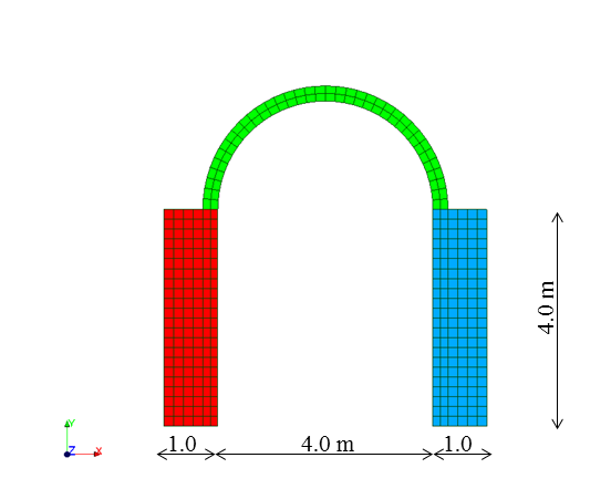
Figure 1: The arch on piers modeled in the experiments. Each differently colored region corresponds to a different material.

Figure 2: The left graph shows the convergence of the objective function to the minimum for each new reduced model generated in the optimization procedure. The dashed line is the tolerance set for the projected gradient in the optimization scheme. The right graph plots the convergence of the frequencies during the process.

Figure 3: The left graph shows the convergence of the objective function to the minimum for each new reduced model generated in the optimization procedure. The dashed line is the tolerance set for the projected gradient in the optimization scheme. The right graph plots the convergence of the frequencies during the process. In this case, the initial points were chosen quite far from the original ones, selecting $E_{2}=2000\ \mathrm{MPa},\rho_{2}=1100\ \mathrm{kg\cdot m^{-3}},E_{3}=1100\ \mathrm{MPa}$.

For the three materials we assume the following values:

$$E_{1} =3250\ \mathrm{MPa} E_{2} =5000\ \mathrm{MPa} E_{3} =4800\ \textrm{MPa}$$

$$\rho_{1} =1800\ \mathrm{\frac{kg}{m^{3}}} \rho_{2} =2200\ \mathrm{\frac{kg}{m^{3}}} \rho_{3} =2100\ \mathrm{\frac{kg}{m^{3}}},$$

where the index $j\in\{1,2,3\}$ indicates the material under consideration. We computed the $5$ leading frequencies by running the NOSA-ITACA code (with these fixed parameters), to obtain:

$$\mathbf{f}\approx\begin{bmatrix}9.575&14.87&23.17&39.17&62.84\end{bmatrix}.$$

Our aim is to validate the optimization method by recovering the original parameters matching these frequencies, assuming $E_{2},\rho_{2}$, and $E_{3}$ are unknown. We consider the following bounds of realistic parameters:

$$1000\ \mathrm{MPa}\leqslant E_{2}\leqslant 9000\ \mathrm{MPa}, 1000\ \mathrm{\frac{kg}{m^{3}}}\leqslant \rho_{2}\leqslant 3000\ \mathrm{\frac{kg}{m^{3}}}, 1000\ \mathrm{MPa} \leqslant E_{3}\leqslant 9000\ \mathrm{MPa},$$

which define the corresponding box $\Omega$ in (4)

In the default implementation, the starting points have been chosen the midpoint of the intervals, which are quite good estimates of the true values. Convergence in this case is displayed in Figure 2. The initial points are sufficiently close to the correct ones for the frequencies to almost match already, and the distance to the optimum during convergence is not easily distinguishable. However, the left plot in Figure 2, which shows the convergence of the objective function in log-scale, clearly demonstrates that we are recovering the right solution.

To test the robustness of the approach, we modified the starting points to be relatively far from the correct ones by making the following choices:

$$E_{2}^{(0)} =2000\ \mathrm{MPa}, \rho_{2}^{(0)} =1100\ \mathrm{\frac{kg}{m^{3}}}, E_{3}^{(0)} =1100\ \mathrm{MPa}.$$

Convergence of the method is displayed in the graphs in Figure 3, which clearly shows that the initial frequencies are quite far from the correct ones; yet the method reaches convergence using only $12$ reduced models. Moreover, a rough estimate (though probably sufficient for most engineering purposes) is already obtained after about 6 steps. Moreover, the Young’s modulus and the mass density of the initial model are recovered exactly up to $5$ digits in this example.

Another important feature for a method that must deal with experimentally measured frequencies is its robustness when the input is subject to noise. In fact, we would expect the frequencies to be accurate only up to a certain relative threshold.

To simulate the behavior of the method in a predictable environment, we perturbed the frequency vector $\hat{\mathbf{f}}=\mathbf{f}+\delta\mathbf{f}$, by imposing $|\delta f_{i}|\leqslant|f_{i}|\cdot\delta$, with $\delta$ the prescribed noise level. We have run tests for $\delta$ ranging from $0.01\%$ to $100\%$: the corresponding error in the retrieved frequencies is plotted in Figure 4.

The error is measured in relative norm, that is we have plotted the infinity norm of the vector with components $(x_{i}-\hat{x}_{i})/x_{i}$, where $x_{i}$ is the vector with the actual model parameters, and $\hat{x}_{i}$ those estimated by the optimization process.

Figure 4: This plot shows the relation between the noise affecting the frequency measurements and the component-wise relative error on the retrieved optimal parameters. The graph shows the linear dependency of the error on the estimated parameters and the noise level of the input data.

The linear behavior of the relative error with respect to the noise level is clearly visible. This behavior suggests that, even if the frequency measurements are contaminated with noise, it is still possible to retrieve meaningful parameters if enough information is provided. Note that, in general, correct (or accurate) recovery of the parameters might not be possible, and a more detailed study of the condition number of this inverse problem will be object of further in-depth study in in future research.

5.3 A dome

Here we provide a more complex example, represented by a dome supported by four 14-meters-high pillars. The dome consists of an octagonal shaped cloister vault 5 meters high, resting on a drum inscribed on a $10\times 11$ meters rectangle. We assume the structure to be composed of 4 different materials: material 1 for the vault (red in Figure 5), material 2 for the top of the drum (blue), material 3 for the lower part of the drum (green) and material 4 for the pillars (gray).

The finite element model consists of $31,052$ elements and $41,245$ nodes. It is modeled using 3D $8$-node hexahedron brick elements, which gives rise to a (projected) model with $122.853$ degrees of freedom.

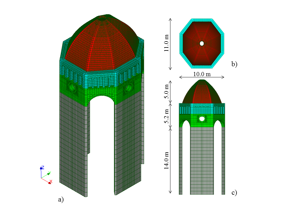
Figure 5: Domed temple

We performed a test similar to that carried out for the arch on piers: we computed the frequencies for a certain choice of parameters, some of which were assumed to be unknown, and ran the optimization scheme trying to recover the original parameters.

In order to obtain the reference frequencies the characteristics of the 4 materials (Young’s modulus and mass density) were set as follows:

$$E_{1} =3000\ \mathrm{MPa} \rho_{1} =1800\ \mathrm{\frac{kg}{m^{3}}} E_{2} =4000\ \mathrm{MPa} \rho_{2} =2000\ \mathrm{\frac{kg}{m^{3}}}$$

$$E_{3} =3500\ \mathrm{MPa} \rho_{3} =1900\ \mathrm{\frac{kg}{m^{3}}} E_{4} =5000\ \mathrm{MPa} \rho_{2} =2200\ \mathrm{\frac{kg}{m^{3}}}$$

$$\nu_{j} =0.25,\qquad j=1,\ldots,4.$$

The leading $10$ frequencies have been computed using the NOSA-ITACA code. The result, expressed in Hertz, are the frequencies in the vector:

$$\mathbf{f}\approx\begin{bmatrix}2.19&2.23&3.76&3.83&4.32&4.60&4.72&8.26&8.30&9.21\end{bmatrix}.$$

The optimization code was run setting the bounds as

$$2000\ \mathrm{MPa}\leqslant E_{j}\leqslant 6000\ \mathrm{MPa}\qquad 1600\ \mathrm{\frac{kg}{m^{3}}}\leqslant\rho_{j}\leqslant 2400\ \mathrm{\frac{kg}{m^{3}}}\qquad j=1,\ldots,4,$$

with the sole exception of $\rho_{3}$ which was set to the correct value. This leaves $7$ parameters to be optimized. No particular starting conditions were specified. In this case, the algorithm chooses the midpoint of the intervals. The convergence history is reported in Figure 6, which reveals that high accuracy is attained with only $4$ outer iterations — with the residual of the objective function being very small even after two steps. The weights have been chosen in order to reach relative accuracy (i.e., $w_{i}=f_{i}^{-1}$) on the target frequencies, with the usual tolerance $\epsilon=10^{-4}$.

Figure 6: Convergence history for the dome model, matching $10$ frequencies with $7$ free parameters. The left plot shows the convergence of the objective function and the norm of the projected gradient, and in the right plot the convergence of frequencies to the exact ones is reported.

The estimated mechanical parameters obtained through the optimization are as follows:

$$E_{1} =2953\ \mathrm{MPa} \rho_{1} =1769\ \mathrm{\frac{kg}{m^{3}}} E_{2} =3932\ \mathrm{MPa} \rho_{2} =1960\ \mathrm{\frac{kg}{m^{3}}}$$

$$E_{3} =3426\ \mathrm{MPa} \rho_{3} =1900\ \mathrm{\frac{kg}{m^{3}}} E_{4} =4951\ \mathrm{MPa} \rho_{2} =2174\ \mathrm{\frac{kg}{m^{3}}}.$$

This corresponds to a relative error between $0.97\%$ and $2.1\%$, with an average of about $1.6\%$. Although such accuracy is a quite good accuracy for practical purposes, even more precise estimates can be obtained by reducing the tolerance to below $10^{-4}$ that we have used in these tests.

5.4 The Clock tower

As a real example, we consider the case study of the Clock tower (“Torre delle Ore”) in Lucca, Italy. The 48.4 m high masonry structure, dating back to the 13th century, has a rectangular cross section of about 5.1$\times$7.1 meters and walls of thickness varying from 1.77 m at the base to 0.85 m at the top. Two barrel vaults are set at heights of about 12.5 m and 42.3 m. The bell chamber is covered by a pavillon roof made up of wooden trusses and rafters. At a height of about 33 m the walls have been instrumented with 4 steel tie rods of 30$\times$30 mm rectangular section. The adjacent buildings abut the tower on two sides for a height of about 13 m and constitute asymmetric boundary conditions. The modal behavior of the tower has already been analyzed using the NOSA-ITACA code and through experimental measurements conducted in November 2016, when the tower was fitted with 4 triaxial seismometric stations. The two procedures yielded similar, albeit not perfectly matching results [32]. Figure 7 shows a picture of the tower, together with the mesh used for its discretization.

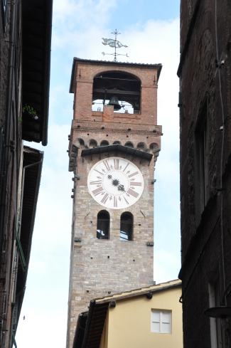
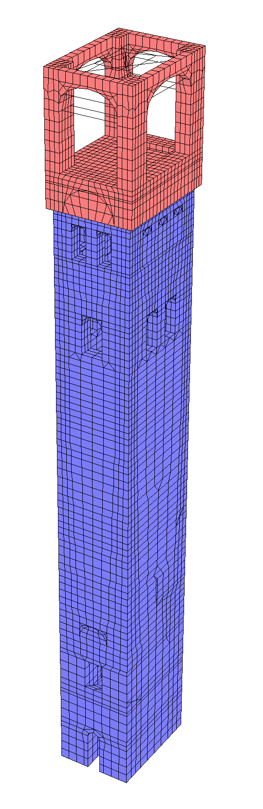
Figure 7: On the left, a picture of the clock tower in Lucca. On the right, the mesh used for the finite element discretization, where the different materials for the bell chamber and the lower part of the tower are reported in different colors (respectively red and light blue).

The frequencies obtained by analyzing data from the fitted instruments via Operational Modal Analysis techniques, are as follows:

$$\mathbf{f}\approx\begin{bmatrix}1.05&1.3&4.19&4.50\end{bmatrix}.$$

The frequencies obtained with the finite element model in [32] are, instead, $[0.98\ 1.24\ 4.32\ 4.38]$. The materials constituting the tower are wood, steel, and masonry, with the latter being different in the bell chamber and the lower part of the tower. The mechanical properties used in the finite element model are

$$E_{w} =10000\ \mathrm{MPa} \rho_{w} =800\ \mathrm{\frac{kg}{m^{3}}} \nu_{w} =0.35$$

$$\rho_{m_{l}} =2100\ \mathrm{\frac{kg}{m^{3}}} \rho_{m_{c}} =1700\ \mathrm{\frac{kg}{m^{3}}} \nu_{m_{l}} =\nu_{m_{c}}=0.2$$

$$E_{s} =$210,000$\ \mathrm{MPa} \rho_{s} =7850\ \mathrm{\frac{kg}{m^{3}}} \nu_{s} =0.3,$$

and we leave the Young’s moduli $E_{m_{c}}$ and $E_{m_{l}}$ as free parameters, since they are not known explicitly due to the lack of experimental information. Here, the subscript $m_{l}$ identifies the lower part of the tower, and $m_{c}$ the bell chamber.

We can reformulate the problem as an optimization one, trying to match the frequencies of the system to the measured ones, allowing the parameters to vary in a reasonable range. In our case we can set

$$2500\ \mathrm{MPa}\leqslant E_{m_{l}}\leqslant 5500\ \mathrm{MPa}\qquad 1000\ \mathrm{MPa}\leqslant E_{m_{c}}\leqslant 5500\ \mathrm{MPa}.$$

As a first test, we choose the weights as the vector of all ones. The convergence of the optimization scheme, obtained with these initial parameters, is reported in Figure 8. Note that the method optimizes the third and fourth frequencies to match quite closely, but at the price of decreasing the quality of the match for the first two (see Table 1).

Figure 8: The left graph reports the convergence history of the objective function to the minimum for each new reduced model generated in the optimization procedure. The norm of the projected gradient is reported as well, and the dashed line is the tolerance of the optimization scheme. The right plot represents the convergence of the frequencies during the process (the dashed lines are the experimental frequencies). Iteration $0$ is the evaluation function at the starting point. In this example, the free parameters are $E_{m_{l}}$ and $E_{m_{c}}$.

Figure 9: The left graph reports the convergence history of the objective function to the minimum for each new reduced model generated in the optimization procedure. The norm of the projected gradient is reported as well, and the dashed line is the tolerance set for the projected gradient in the optimization scheme. The right plot represents the convergence of the frequencies during the process (the dashed line are the experimental frequencies). Iteration $0$ is the evaluation function at the starting point. In this example, the free parameters are $E_{m_{l}}$ and $E_{m_{c}}$, and the objective function is defined using the weights $w_{i}=f_{i}^{-1}$.

This is connected to the choice of $\mathbf{w}$, which ensures norm-wise accuracy, but not a relative one. Often, we prefer to have a low relative error on the frequencies, instead of an absolute one. Therefore, it is natural to choose $w_{i}=f_{i}^{-1}$ (in fact, this is the default choice in the implementation). This yields different results, and different approximations for both the parameters and the frequencies. More specifically, we expect a better match on the lowest end of the spectrum, and a worse one on the highest frequencies.

The convergence history with this choice of $\mathbf{w}$ is reported in Figure 9, and the results are shown in Table 1. It appears immediately evident that the relative errors are balanced with $w_{i}=f_{i}^{-1}$, whereas they tend to increase on the small frequencies when $w_{i}=1$.

The parameters identified by the model updating phase give $E_{m_{l}}\approx$3182$\ \mathrm{MPa}$ and $E_{m_{c}}\approx$1873$\ \mathrm{MPa}$ when using weights equal to one, and $E_{m_{l}}\approx$3076$\ \mathrm{MPa}$ and $E_{m_{c}}\approx$1950$\ \mathrm{MPa}$ when aiming for relative accuracy.

We conclude this section by comparing the overall CPU time of our implementation with those of alternative solvers, which in various ways fail to exploit the problem structure. Table 2 compares 4 different implementations:

RM

This implementation corresponds to the current proposal, that is, a solver based on the trust-region and projection approach described in the previous section and used in the tests presented herein. This strategy is labeled as “RM” in the table — highlighted with the bold font.

BB

Here we interpret the finite element code as a black-box function and solve the optimization problem using a general purpose optimizer. This is done to reflect a scenario in which the user has no access to the internals of the finite element code — and requires an assembly phase at every function evaluation. Derivatives are computed here by finite differences. This is column “BB” in the table.

A

In this approach, we separately assemble the parametric generalized eigenvalue problem $K(\mathbf{x})-\lambda M(\mathbf{x})$ and then pass to a general optimizer a function that evaluates the frequencies for a given value of $\mathbf{x}$. This function corresponds to the Lanczos projection routine used internally in RM. Derivatives are computed here by finite differences. This is approach “A” in the table.

AD

The same as A, but derivatives are evaluated analytically as described to Section 4.3.3. This is “AD” in the table.

The general optimizer chosen for the BB, A and AD implementations is again fmincon with the sqp option available in the Optimization toolbox of MATLAB. In our experience, this choice turns out to be the most efficient among those available in the toolbox. This same function has been used for computation of the step in the trust-region scheme of Algorithm 1.

In Table 2, the time for assembly (which needs to be added to the costs in columns A, AD, and RM) is reported separately, as well as the problem’s degrees of freedom.

It is immediately apparent that the proposed RM method is the fastest in all cases except the arch on piers, where given the small dimension incurs in some overhead. Moreover, it is worth stressing that our approach exhibits a complexity that seems to grow nicely with the dimension. The general optimization approach BB, instead, becomes costly when the number of degrees of freedom increases.

For instance, in the dome example, the timings range from about 7 hours for BB to slightly more than 3 minutes with our approach. The case where we supply derivatives to the optimizer (AD) still takes more than 30 minutes.

Exp. freq.	Freq. ($w_{i}=1$)	Rel. error ($w_{i}=1)$	Freq. ($w_{i}=f_{i}^{-1}$)	Rel. error ($w_{i}=f_{i}^{-1}$)
$1.05$ Hz	$1.0621$ Hz	$1.15$%	$1.0449$ Hz	$0.49$%
$1.30$ Hz	$1.3366$ Hz	$2.82$%	$1.315$ Hz	$1.15$%
$4.19$ Hz	$4.2041$ Hz	$0.33$%	$4.2154$ Hz	$0.61$%
$4.50$ Hz	$4.4729$ Hz	$0.60$%	$4.4409$ Hz	$1.31$%

Table 1: Frequencies and corresponding relative errors computed using the weights $w_{i}=1$ and $w_{i}=f_{i}^{-1}$ for the problem of the clock tower in Lucca, Italy.

	# dof	BB	A	AD	RM	Assembly
Arch on piers	851	16.40s	1.17s	0.62s	0.68s	0.42s
Dome	122,853	25,032s	7,662.4s	1,990.5s	226.02s	134.32s
Clock tower	45,511	476.9s	305.39s	202.87s	44.10s	32.22s

Table 2: Timings for different optimization approaches. The timings reported for the approaches “Assembled” (A), “Assembled $+$ derivatives” (AD), and “Reduced model” (RM) do not include the time needed to assembly the parametric finite element model, which is reported in the last column. The Portal model has been run with the default starting points.

The timings suggest the unsurprising conclusion that better knowledge of the underlying optimization problem leads to more efficient and faster optimization routines. It should be noted that the stopping criterion for all the approaches is set to ensure that the first order optimality condition (given by the norm of the projected gradient) is smaller than $\epsilon=10^{-4}$ used in the experiments. All the approaches provide solutions with comparable accuracy.

6 Concluding remarks

In this work we have presented a model updating scheme focusing on the optimization of finite element models for structural dynamics. We have shown how the subspace projection method used to compute the eigenvalues at the lowest end of the spectrum can be used directly as a parametric model order reduction step, and that embedding it in a trust-region scheme can be very effective.

Several examples have been reported on, both to test the theoretical properties of the scheme as well as to demonstrate its practical applicability. We have also presented a preliminary numerical evidence of its robustness against perturbations in the data, an aspect which will be further investigated and characterized in future work.

We believe that embedding the model updating step directly in the finite element code naturally leads to more efficient procedures, compared to applying an optimizer fed with a black-box finite element code. The proposed approach can benefit from the fact that the optimizer knows the details about the finite element formulation, and this reveals to be particularly effective in terms of reliability and efficiency.

Several problems remain open, and deserve further study in the future. For instance, optimization of mode shapes — and not only eigenfrequencies — is of crucial importance to obtain an accurate understanding of the dynamic behavior of a structure.

Moreover, a robust and efficient implementation of the approach within the NOSA-ITACA code needs to be performed — along with its integration with the graphical user interface based on SALOME. These issues will be addressed in future work.

References

References

- Agarwal and Biegler [2013] Agarwal, A., Biegler, L. T., 2013. A trust-region framework for constrained optimization using reduced order modeling. Optimization and Engineering 14 (1), 3–35.
- Alexandrov and Dennis [1995] Alexandrov, N., Dennis, J. E., 1995. Multilevel algorithms for nonlinear optmization. Optimal design and control, 1–22.
- Amsallem et al. [2015] Amsallem, D., Zahr, M., Choi, Y., Farhat, C., 2015. Design optimization using hyper-reduced-order models. Structural and Multidisciplinary Optimization 51 (4), 919–940.
- Aoki et al. [2007] Aoki, T., Sabia, D., Rivella, D., Komiyama, T., 2007. Structural characterization of a stone arch bridge by experimental tests and numerical model updating. International Journal of Architectural Heritage 1 (3), 227–250.
- Araújo et al. [2012] Araújo, A. S., Lourenço, P. B., Oliveira, D. V., Leite, J. C., 2012. Seismic assessment of st. james church by means of pushover analysis: before and after the new zealand earthquake. The Open Civil Engineering Journal 6, 160–172.
- Azzara et al. [2016] Azzara, R., De Roeck, G., Reynders, E., Girardi, M., Padovani, C., Pellegrini, D., 2016. Assessment of the dynamic behaviour of an ancient masonry tower in lucca via ambient vibrations. In: Proceedings of the 10th international conference on the Analysis of Historican Contructions-SAHC 2016. CRC Press, pp. 669–675.
- Azzara et al. [2018] Azzara, R. M., De Roeck, G., Girardi, M., Padovani, C., Pellegrini, D., Reynders, E., 2018. The influence of environmental parameters on the dynamic behaviour of the san frediano bell tower in lucca. Engineering Structures 156, 175–187.
- Bai [2002] Bai, Z., 2002. Krylov subspace techniques for reduced-order modeling of large-scale dynamical systems. Applied numerical mathematics 43 (1-2), 9–44.
- Bathe and Wilson [1976] Bathe, K.-J., Wilson, E. L., 1976. Numerical methods in finite element analysis. Vol. 197. Prentice-Hall Englewood Cliffs, NJ.
- Benner et al. [2015] Benner, P., Gugercin, S., Willcox, K., 2015. A survey of projection-based model reduction methods for parametric dynamical systems. SIAM review 57 (4), 483–531.
- Binante et al. [2017] Binante, V., Girardi, M., Padovani, C., Pasquinelli, G., Pellegrini, D., Porcelli, M., Robol, L., 2017. NOSA-ITACA 1.1 Documentation.
- Cabboi et al. [2017] Cabboi, A., Gentile, C., Saisi, A., 2017. From continuous vibration monitoring to fem-based damage assessment: Application on a stone-masonry tower. Construction and Building Materials 156, 252–265.
- Ceravolo et al. [2016] Ceravolo, R., Pistone, G., Fragonara, L. Z., Massetto, S., Abbiati, G., 2016. Vibration-based monitoring and diagnosis of cultural heritage: a methodological discussion in three examples. International Journal of Architectural Heritage 10 (4), 375–395.
- Chen and Garba [1980] Chen, J. C., Garba, J. A., 1980. Analytical model improvement using modal test results. AIAA journal 18 (6), 684–690.
- Compán et al. [2017] Compán, V., Pachón, P., Cámara, M., Lourenço, P. B., Sáez, A., 2017. Structural safety assessment of geometrically complex masonry vaults by non-linear analysis. the chapel of the würzburg residence (germany). Engineering Structures 140, 1–13.
- Conn et al. [1988] Conn, A. R., Gould, N. I., Toint, P. L., 1988. Global convergence of a class of trust region algorithms for optimization with simple bounds. SIAM journal on numerical analysis 25 (2), 433–460.
- Conn et al. [2000] Conn, A. R., Gould, N. I., Toint, P. L., 2000. Trust region methods. SIAM.
- Demmel [1997] Demmel, 1997. Applied numerical linear algebra. SIAM.
- Douglas and Reid [1982] Douglas, B. M., Reid, W. H., 1982. Dynamic tests and system identification of bridges. Journal of the Structural Division 108 (ST10).
-
Erdogan [2017]
Erdogan, Y. S., 2017. Discrete and continuous finite element models and their
calibration via vibration and material tests for the seismic assessment of
masonry structures. International Journal of Architectural Heritage 11 (7),
1026–1045.
URL https://doi.org/10.1080/15583058.2017.1332255 - Ericsson and Ruhe [1980] Ericsson, T., Ruhe, A., 1980. The spectral transformation lanczos method for the numerical solution of large sparse generalized symmetric eigenvalue problems. Mathematics of Computation 35 (152), 1251–1268.
- Fragonara et al. [2017] Fragonara, L. Z., Boscato, G., Ceravolo, R., Russo, S., Ientile, S., Pecorelli, M. L., Quattrone, A., 2017. Dynamic investigation on the mirandola bell tower in post-earthquake scenarios. Bulletin of Earthquake Engineering 15 (1), 313–337.
- Friswell and Mottershead [2013] Friswell, M., Mottershead, J. E., 2013. Finite element model updating in structural dynamics. Vol. 38. Springer Science & Business Media.
- Gentile and Saisi [2007] Gentile, C., Saisi, A., 2007. Ambient vibration testing of historic masonry towers for structural identification and damage assessment. Construction and Building Materials 21 (6), 1311–1321.
- Giunta and Eldred [2000] Giunta, A., Eldred, M., 2000. Implementation of a trust region model management strategy in the dakota optimization toolkit. In: 8th Symposium on Multidisciplinary Analysis and Optimization. p. 4935.
- Kato [2013] Kato, T., 2013. Perturbation theory for linear operators. Vol. 132. Springer Science & Business Media.
- Kocaturk et al. [2017] Kocaturk, T., Erdogan, Y., Demir, C., Gokce, A., Ulukaya, S., Yuzer, N., 2017. Investigation of existing damage mechanism and retrofitting of skeuophylakion under seismic loads. Engineering Structures 137, 125–144.
- Lehoucq et al. [1998] Lehoucq, R. B., Sorensen, D. C., Yang, C., 1998. ARPACK users’ guide: solution of large-scale eigenvalue problems with implicitly restarted Arnoldi methods. SIAM.
- Marwala [2010] Marwala, T., 2010. Finite element model updating using computational intelligence techniques: applications to structural dynamics. Springer Science & Business Media.
- O’Connell et al. [2017] O’Connell, M., Kilmer, M. E., de Sturler, E., Gugercin, S., 2017. Computing reduced order models via inner-outer krylov recycling in diffuse optical tomography. SIAM Journal on Scientific Computing 39 (2), B272–B297.
- Parks et al. [2006] Parks, M. L., De Sturler, E., Mackey, G., Johnson, D. D., Maiti, S., 2006. Recycling krylov subspaces for sequences of linear systems. SIAM Journal on Scientific Computing 28 (5), 1651–1674.
- Pellegrini et al. [2017] Pellegrini, D., Girardi, M., Padovani, C., Azzara, R., 2017. A new numerical procedure for assessing the dynamic behaviour of ancient masonry towers. In: Proceedings of the 6th ECCOMAS Thematic Conference on Computational Methods in Structural Dynamics and Earthquake Engineering - COMPDYN 2017. pp. –.
- Pérez-Gracia et al. [2011] Pérez-Gracia, V., Di Capua, D., Caselles, O., Rial, F., Lorenzo, H., Gonzalez-Drigo, R., Armesto, J., 2011. Characterization of a romanesque bridge in galicia (spain). International Journal of Architectural Heritage 5 (3), 251–263.
- Porcelli [2013] Porcelli, M., 2013. On the convergence of an inexact gauss–newton trust-region method for nonlinear least-squares problems with simple bounds. Optimization Letters 7 (3), 447–465.
- Porcelli et al. [2015] Porcelli, M., Binante, V., Girardi, M., Padovani, C., Pasquinelli, G., 2015. A solution procedure for constrained eigenvalue problems and its application within the structural finite-element code nosa-itaca. Calcolo 52 (2), 167–186.
- Qian et al. [2017] Qian, E., Grepl, M., Veroy, K., Willcox, K., 2017. A certified trust region reduced basis approach to PDE-constrained optimization. SIAM Journal on Scientific Computing 39 (5), S434–S460.
- Ramos et al. [2011] Ramos, L. F., Alaboz, M., Aguilar, R., Lourenço, P. B., 2011. Dynamic identification and fe updating of s. torcato church, portugal. In: Dynamics of Civil Structures, Volume 4. Springer, pp. 71–80.
- Ramos et al. [2010] Ramos, L. F., Marques, L., Lourenço, P. B., De Roeck, G., Campos-Costa, A., Roque, J., 2010. Monitoring historical masonry structures with operational modal analysis: two case studies. Mechanical systems and signal processing 24 (5), 1291–1305.
- Simoen et al. [2015] Simoen, E., De Roeck, G., Lombaert, G., 2015. Dealing with uncertainty in model updating for damage assessment: A review. Mechanical Systems and Signal Processing 56, 123–149.
- Soodhalter et al. [2014] Soodhalter, K. M., Szyld, D. B., Xue, F., 2014. Krylov subspace recycling for sequences of shifted linear systems. Applied Numerical Mathematics 81, 105–118.
- Sun [1990] Sun, J.-g., 1990. Multiple eigenvalue sensitivity analysis. Linear algebra and its applications 137, 183–211.
- Teughels and De Roeck [2005] Teughels, A., De Roeck, G., 2005. Damage detection and parameter identification by finite element model updating. Revue européenne de génie civil 9 (1-2), 109–158.
- Torres et al. [2017] Torres, W., Almazán, J. L., Sandoval, C., Boroschek, R., 2017. Operational modal analysis and fe model updating of the metropolitan cathedral of santiago, chile. Engineering Structures 143, 169–188.
- Yue and Meerbergen [2013] Yue, Y., Meerbergen, K., 2013. Accelerating optimization of parametric linear systems by model order reduction. SIAM Journal on Optimization 23 (2), 1344–1370.
- Zahr and Farhat [2015] Zahr, M. J., Farhat, C., 2015. Progressive construction of a parametric reduced-order model for PDE-constrained optimization. International Journal for Numerical Methods in Engineering 102 (5), 1111–1135.