Experimental demonstration of time-frequency duality of biphotons

Abstract

Time-frequency duality, which enables control of optical waveforms by manipulating amplitudes and phases of electromagnetic fields, plays a pivotal role in a wide range of modern optics. The conventional one-dimensional (1D) time-frequency duality has been successfully applied to characterize the behavior of classical light, such as ultrafast optical pulses from a laser. However, the 1D treatment is not enough to characterize quantum mechanical correlations in the time-frequency behavior of multiple photons, such as the biphotons from parametric down conversion. The two-dimensional treatment is essentially required, but has not been fully demonstrated yet due to the technical problem. Here, we study the two-dimensional (2D) time-frequency duality duality of biphotons, by measuring two-photon distributions in both frequency and time domains. It was found that generated biphotons satisfy the Fourier limited condition quantum mechanically, but not classically, by analyzing the time-bandwidth products in the 2D Fourier transform. Our study provides an essential and deeper understanding of light beyond classical wave optics, and opens up new possibilities for optical synthesis in a high-dimensional frequency space in a quantum manner.

Introduction Optical studies that utilize the relationship coupled by Fourier transform are called Fourier optics, and form a wide range of optical science and technology fields, including optical imaging Stark (1982); Goodman (2017); Zhang et al. (2014), spectroscopy Smith (2011); Bell (1972), optical measurement Sirohi (2017); Griffiths and De Haseth (2007), and optical signal processing VanderLugt (2005); Rhodes (2009). In particular, it is well-known that each electric field distribution in the time and frequency domains is connected by the one-dimensional Fourier transform (1DFT)

$$A^{(1)}(t)=\frac{1}{\sqrt{2\pi}}\int d\nu\tilde{A}^{(1)}(\nu)e^{-2\pi i\nu\,t}$$ (1)

where $A^{(1)}(t)$ is the electric field amplitude as a function of time $t$, and $\tilde{A}^{(1)}(\nu)$ is the corresponding distribution with a frequency $\nu$, as shown in Fig. 1(a). This relationship is a fundamental principle of cutting-edge technologies on an ultrashort pulse laser, as seen in the recent developments in optical synthesis Chan et al. (2011); Suhaimi et al. (2015). On the other hand, Fourier optical phenomena can also be explained from the viewpoint of the particle nature of light, i.e., the photon. Since the photons contained in a laser light pulse have no quantum correlation, the collective behavior of a many-photon system can be handled as a single-photon problem Kocsis et al. (2011); Aspden et al. (2016). As a result, the quantum mechanical treatment between the time and frequency domains of a laser light pulse can be explained by 1DFT, producing results in equivalent to an understanding with classical wave optics. However, in principle, these phenomena should be treated as a quantum many-body system, because a large number of photons are contained in an optical pulse output from an ultrashort pulse laser.

Recent progress in quantum optical technologies allows us to control not only a number of photons (i.e., photon statistics), but also the frequency quantum correlations in an optical pulse Eckstein et al. (2011); Jin et al. (2016); Chen et al. (2017); Jin et al. (2017). Such a frequency quantum correlation would affect its temporal distribution directly through the time-frequency duality. It is not reasonable to treat the behavior of a quantum-mechanically correlated photon as a single-photon (or 1D) problem. Therefore, an optical pulse containing the correlated photons requires a higher-order Fourier treatment that incorporates the quantum mechanics. As the first step toward future photonics at the single-photon level in the time-frequency domain, we focus here on the time-frequency behavior of biphotons, which requires the treatment of the two-dimensional Fourier transform (2DFT), as shown in Figs. 1b, c.

$$A^{(2)}(t_{1},t_{2})=\frac{1}{2\pi}\int\int d\nu_{1}d\nu_{2}\tilde{A}^{(2)}(\nu_{1},\nu_{2})e^{-2\pi i(\nu_{1}\,t_{1}+\nu_{2}\,t_{2})}$$ (2)

where $A^{(2)}(t_{1},t_{2})$ is the biphoton probability amplitude at time $t_{1}$ and $t_{2}$, and $\tilde{A}^{(2)}(\nu_{1},\nu_{2})$ is the corresponding distribution with the frequency $\nu_{1}$ and $\nu_{2}$.

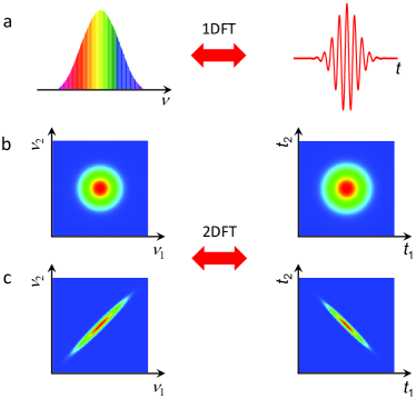
Figure 1: Conceptual drawing of 1- and 2D treatments for the time-frequency duality. (a) Classical duality in the time-frequency domains; a broader distribution in the frequency domain results in a narrower distribution in the time domain; (b) 2D Fourier transform for a frequency-uncorrelated biphoton; frequency uncorrelation leads to uncorrelation in the time domain; (c) 2D Fourier transform of a biphoton with positive frequency correlation; correlations are inverted between the time and frequency domains.

From the early stage of quantum optical experiments, time-frequency correlation of biphotons generated from spontaneous parametric down-conversion process have been extensively investigated Burnham and Weinberg (1970); Hong et al. (1987); Larchuk et al. (1993); Shih et al. (1994); Giovannetti et al. (2002); Jin and Shimizu (2018); Kim and Grice (2005); Shimizu and Edamatsu (2009); Avenhaus et al. (2009); Fang et al. (2014); Allgaier et al. (2017); Kuzucu et al. (2008a); Cho et al. (2014). In these studies, they discussed the relationship between a classical frequency spectrum and time-domain quantum interference patterns Hong et al. (1987); Larchuk et al. (1993); Shih et al. (1994); Giovannetti et al. (2002); Jin and Shimizu (2018), the spectral properties Kim and Grice (2005); Shimizu and Edamatsu (2009); Avenhaus et al. (2009); Fang et al. (2014), or the temporal Allgaier et al. (2017); Kuzucu et al. (2008a); Cho et al. (2014) properties of biphotons. These studies provide partial understanding of nonclassical behavior of biphotons. However, it is necessary to discuss in the two-dimensional time-frequency space for the comprehensive understanding of biphoton behavior, but still has not been fully demonstrated yet due to the technical problem. Here, we experimentally demonstrate the time-frequency duality of biphotons with the positive frequency correlations, by measuring both the two-photon spectral intensity distribution (TSI) and the two-photon temporal intensity distribution (TTI). Furthermore, we show the variation of two-photon temporal distributions as a result of the two-photon spectral modulations, keeping quantum optical-Fourier-transform limited conditions.

Results To generate biphotons with positive frequency correlation, we exploit the spontaneous parametric down-conversion process in a periodically poled potassium titanyl phosphate (PPKTP) crystal pumped by a mode-locked titanium sapphire laser, operating at the center wavelength of 792 nm. Thanks to the group velocity matching condition König and Wong (2004); Jin et al. (2013) with the femtosecond laser pulse pumping, we could generate biphotons with positive frequency correlations at the center wavelength of 1584 nm (see Supplementary Information for details). Since biphotons generated via the type-II phase-matching condition have orthogonal polarizations, the polarization of the constituent photons were aligned along either the crystallographic y- or z- axis. To manipulate a two-photon spectral distribution, we used pump pulses with a bandwidth of either 8.1 or 2.8 nm. In addition, we prepared two PPTKP crystals, one 30-mm and the other 10-mm long, and positioned one or the other in our experimental apparatus (see Methods).

We performed two experiments to characterize the biphoton distributions in the time-frequency domain. A two-photon spectrometer consisting of two tunable bandpass filters, which had a Gaussian-shaped filter function with a fixed FWHM of 0.56 nm, and a tunable central wavelength from 1560-1620 nm, followed by a two-photon detector enabled us to conduct the TSI measurements Shimizu and Edamatsu (2009); Jin et al. (2013). For the TTI measurements, we utilized a time-resolved upconversion detection system with a spatial multiplexing technique Kuzucu et al. (2008b, a). The TTI was measured by scanning the temporal delay between the constituent photons and the local oscillator pulse coming from the mode-locked laser with a step length of 0.13 ps, and we recorded coincidence events (see Methods).

Figure 2 shows the experimentally measured TSIs (left) and TTIs (right) with a combination of the two different pump bandwidths (2.8 or 8.1 nm) and two different crystal lengths (10 or 30 mm). We reproduced TSIs and TTIs deconvoluted from the original data, taking into account the resolutions of our two-photon detection systems (see Methods).

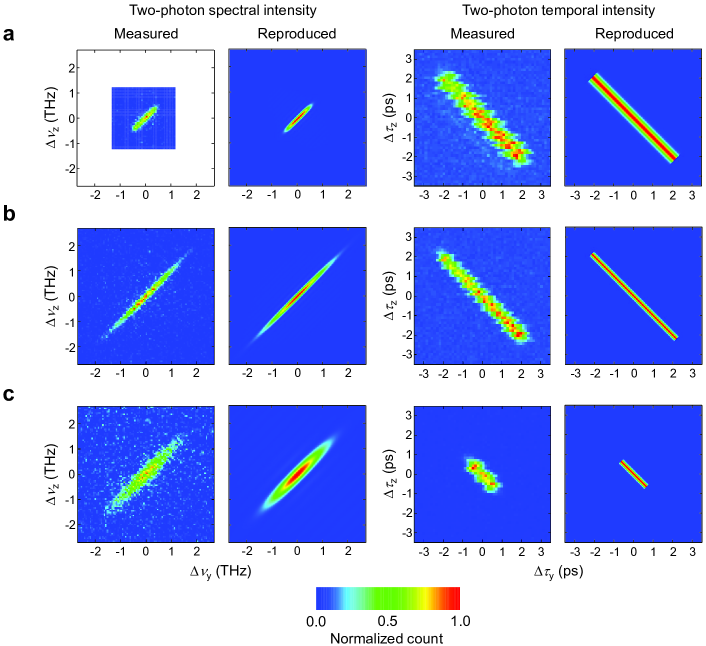
Figure 2: Observation of time-frequency duality of biphotons. The plots in the left two columns are TSIs, and those in the right two columns are the TTIs. No measurements were carried out in the white area in (a). The biphotons were produced under different conditions. (a) The pump had a near-rectangular profile with a bandwidth $\Delta\lambda_{p}$ of 2.8 nm and PPKTP crystal length $L$ of 30 mm; (b) the pump had a Gaussian profile with a bandwidth $\Delta\lambda_{p}$ of 8.1 nm and $L$ of 30 mm; (c) the pump also had a Gaussian profile with a bandwidth $\Delta\lambda_{p}$ of 8.1 nm and $L$ of 10 mm. The temporal distributions varied by manipulating the spectral distributions.

In Fig. 2, the horizontal (vertical) axis $\Delta\nu_{y}$ ($\Delta\nu_{z}$) is the frequency-shift from the center frequency of each distribution in the y- (z-)direction-polarized photons. The zero-shifted frequencies are 189.4 THz, corresponding to a center wavelength of 1584 nm. The specific features of the time-frequency duality of the biphotons can be clearly observed in Fig. 2; the TSI of the biphotons from the PPKTP crystal has a positively correlated distribution along the diagonal ($\Delta\nu_{y}=\Delta\nu_{z}$) direction, while the corresponding TTI has a negatively correlated distribution along the anti-diagonal ($\Delta\nu_{y}=-\Delta\nu_{z}$) direction.

When the pump bandwidth was increased from 2.8 nm in Fig. 2a to 8.1 nm in Fig. 2b for the fixed crystal length of 30 mm, the TSI became slightly broader along the diagonal direction, while the width was unchanged along the anti-diagonal direction. In the same manner, when the crystal length $L$ was shortened from 30 mm in Fig. 2b to 10 mm in Fig. 2c, the TSI became broader along the anti-diagonal direction, while staying the same in the diagonal direction. We can understand these phenomena from the following facts: the biphoton spectral amplitude $\tilde{A}^{(2)}(\Delta\nu_{y},\Delta\nu_{z})$ is the product of a phase-matching function $\Phi(\nu_{-},L)$ and a pump spectral function $\alpha(\nu_{+})$; $\tilde{A}^{(2)}(\nu_{+},\nu_{-})=\Phi(\nu_{-},L)\alpha(\nu_{+})$, where $\nu_{\pm}=\frac{1}{\sqrt{2}}(\Delta\nu_{y}-\Delta\nu_{z})$ and $L$ is the given PPKTP length. Therefore the bandwidth of the TSI in the $\nu_{+}$ direction is determined by the spectral function of the pump laser, while that in the $\nu_{-}$ direction is determined by the phase-matching function depending on the crystal length $L$ (seeSupplementary Information). Thus, in our case, the time-frequency duality of the biphoton can be expressed in the following form:

$$A^{(2)}(\Delta\tau_{y},\Delta\tau_{z}) = \frac{1}{\sqrt{2\pi}}\int d\nu_{+}\alpha(\nu_{+})e^{-2\pi i\nu_{+}\tau_{+}}$$ (3)

$${}\times\frac{1}{\sqrt{2\pi}}\int d\nu_{-}\Phi(\nu_{-},L)e^{-2\pi i\nu_{-}\tau_{-}}$$

$$= A^{(1)}_{1}(\tau_{+})A^{(1)}_{1}(\tau_{-}).$$

where $\tau_{\pm}=\frac{1}{\sqrt{2}}(\Delta\tau_{y}\pm\Delta\tau_{z})$. This indicates that the 2DFT can be decomposed into the product of two 1DFTs: $A^{(1)}_{1}(\tau_{+})=\frac{1}{\sqrt{2\pi}}\int d\nu_{+}\alpha(\nu_{+})e^{-2\pi i\nu_{+}\tau_{+}}$ and $A^{(1)}_{2}(\tau_{-})=\frac{1}{\sqrt{2\pi}}\int d\nu_{-}\Phi(\nu_{-},L)e^{-2\pi i\nu_{-}\tau_{-}}$. Based on this, we confirmed the time-bandwidth product (TBP) between $\delta\tau_{+}$ and $\delta\nu_{+}$ or $\delta\tau_{-}$ and $\delta\nu_{-}$, where $\delta\tau_{\pm}$ ($\delta\nu_{\pm}$) is the full width at half maximum (FWHM) values along the $\tau_{\pm}$ ($\nu_{\pm}$) directions in the TTIs (the TSIs).

Using the reproduced data in Fig. 2, we estimated $\delta\nu_{\pm}$ and $\delta\tau_{\pm}$ for all the cases in Fig. 2 and calculated TBPs. It is worth evaluating the TBP for the marginal distributions, as shown in Fig. 3, because they can be observed by classical spectroscopic measurements. Here, $\delta\nu_{y}(\delta\tau_{y})$ is the FWHM of the marginal distribution of the TSI (TTI) after the deconvolution. All TBP values are summarized in Table  1.

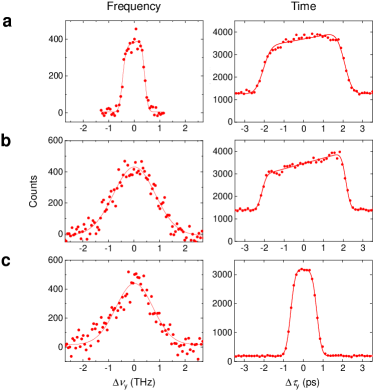
Figure 3: Marginal distributions of two photon spectral and temporal intensity distributions. Left graphs are the marginal distributions of TSIs, shown in Fig. 2, projecting onto the $\Delta\nu_{y}$ axis. Right graphs are those of TTIs, projecting onto the $\Delta\tau_{y}$ axis. The red lines represent a least-square fit to the data. Back ground counts exist in the TTI measurements due to the unwanted photon pair generation in the upconversion crystal. No relations are observed for corresponding distributions between the time and frequency domains.

It is obvious that the TBP values between $\delta\tau_{\pm}$ and $\delta\nu_{\pm}$ are less than 1, meaning that the generated biphoton wave packets satisfy the nearly Fourier transform limited condition. The values of $\delta\nu_{+}\times\delta\tau_{+}$ are almost determined by the pump pulse spectra $\alpha(\nu_{+})$, and would have the value of approximately 0.44 when assuming a Gaussian. On the other hand, $\delta\nu_{-}\times\delta\tau_{-}$ is associated with the phase-matching function $\Phi(\nu_{-},L)$, and the values would be approximately 0.87 due to the rectangular shape of the PPKTP crystals along the propagation direction of the pump pulse. However, the value of $\delta\nu_{y}\times\delta\tau_{y}$ in Table  1 is clearly larger than 1. This implies that the constituent photons of the biphoton wave packet no-longer satisfy the Fourier transform limited conditions (i.e., the coherence of single-photon wave packets are degraded). The disappearance of the single-photon coherence is the inherent characteristics in a quantum-mechanical biparticle system and is well-known as the degradation of purity in a qubit system Nielsen and Chuang (2000).

Discussion We now consider the difference of time-frequency duality between classical and quantum regimes. It is known that the Hamiltonian for a classical electromagnetic wave can be written as the sum of Hamiltonians for independent harmonic oscillators. Thus, in terms of the photon picture, we can interpret classical optical phenomena as the collective behavior of uncorrelated photons, which results in a single photon (1D) treatment. Under the 1D treatment, we understand the electric field amplitude, or one-photon probability amplitude, between time and frequency domains are conjugate physical quantities. In contrast, the limitation of the 1D treatment is evident from the results presented in Figs. 2 and 3. In practice, the TBP of $\delta\nu_{y}\times\delta\tau_{y}$ implies the single-photon spectrum associated with the marginal distribution in the frequency domain is no longer conjugate with the single-photon temporal shape. In our case, it is obvious that the marginal distributions in the frequency domain is mostly determined by the distribution along the diagonal direction in the TSIs, whose Fourier conjugate pair is the distribution along the diagonal direction in the time domain. In other words, the single-photon spectral distribution strongly affects the temporal quantum correlation of the biphoton. In the same manner, the frequency quantum correlation leads to the single-photon temporal distribution. Through these considerations, we can understand classical optical theory only does not cause inconsistency for the collective behavior of uncorrelated photon such as laser pulses. Higher-order treatments incorporates the quantum mechanics, such as a quantum many-body system Schweigler et al. (2017), is essentially required for general understanding the nature of light.

	$\Delta\lambda_{p}$	$L$	$\delta\tau_{+}\times\delta\nu_{+}$	$\delta\tau_{-}\times\delta\nu_{-}$	$\delta\tau_{y}\times\delta\nu_{y}$
a	2.8 nm	30 mm	0.46	0.77	3.4
b	8.1 nm	30 mm	0.49	0.85	8.2
c	8.1 nm	10 mm	0.41	0.59	2.2

Table 1: Time-bandwidth products of the biphoton wave packets. Summary of the time-bandwidth products in three experimental conditions in Fig. 2. All the values are less than 1 in the two-photon distributions, implying biphotons nearly satisfy the Fourier-limited conditions. On the other hand, time-bandwidth product values in the marginal distributions clearly donot meet the Fourier-limited condition.

As a many-body quantum system, our study opens up possible new directions for optical science and technologies, taking into account the quantum correlation, which classical optics treats as the collective motion of uncorrelated photons. Specifically, time-frequency duality with the higher-dimensional treatments has great potential to manage a multiple-photon wave packet in a higher dimensional time-frequency space. Here, we only manipulated the real part of the two-photon spectral amplitude (i.e., the TSI). By modulating an imaginary two-photon spectral amplitude, i.e., the phase between two-photon spectral modes, in addition to the real part, however, we could easily extent our work to a new quantum optical synthesis technology based on a 2D Fourier optical treatment. This may lead to a deeper understanding of the essential nature of light and to the development of future photonics at the single-photon level in the time-frequency domain.

Conclusion In summary, we have demonstrated the correlation inversion between time and frequency domains for frequency-positive-correlated biphotons, by experimentally measuring two-photon distributions in both domains. It was discovered that the generated biphotons satisfy the Fourier limited condition quantum mechanically, but not classically. Our study opens up possible new directions for optical science and technologies a many-body and high-dimensional frequency space.

Acknowledgements We thank Y. Guo for the helpful discussions. R.J. is supported by a fund from the Educational Department of Hubei Province, China (Grant No. D20161504), and by National Natural Science Foundations of China (Grant No.11704290). R.S. acknowledges support from the Research Foundation for Opto-Science and Technology, Hamamatsu, Japan, and support from Matsuo Foundation, Tokyo, Japan.

Methods

Schematic illustration of the whole experimental setup The experiment setup is shown in Fig. 4. We used femtosecond laser pulses with a repetition rate of 76 MHz from a mode-locked titanium sapphire laser, operating at the center wavelength of 792 nm with a bandwidth of 8.1 nm. These were divided into two paths by a polarization beam splitter (PBS) in order to generate and detect biphotons. For the biphoton generation, pulses were sent to a periodically poled potassium titanyl phosphate (PPKTP) crystal with a poling period of 46.1 $\mu$m for type-II group-velocity-matched spontaneous parametric down-conversion. To manipulate the two-photon spectral distribution, we also prepared the pump pulse with a bandwidth of 2.8 nm (by inserting a bandpass filter), and crystals of 30 and 10 mm in length. Thanks to the group velocity matching condition with the femtosecond laser pulse pumping, we could generate biphotons with positive frequency correlations at the center wavelength of 1584 nm. Since biphotons generated via the type-II phase-matching condition have orthogonal polarizations, the polarization of the constituent photons were aligned along either the crystallographic y- or z-axis. The constituent photons were separated by a PBS and coupled into two polarization-maintaining fibers (PMF). The other path of the pump laser pulse was spatially filtered, and then used as a local oscillator (LO) for TTI measurement. For TSI measurement Shimizu and Edamatsu (2009); Jin et al. (2013) , each constituent photon of the biphoton was sent to tunable bandpass filters (BPFs), which had a Gaussian-shaped filter function with a fixed FWHM of 0.56 nm and a tunable central wavelength from 1560-1620 nm, followed by a two-photon detector consisting of two fiber-coupled single-photon detectors and a time interval analyzer (TIA). The TSI was measured by scanning the central wavelength of the two BPFs with a step length of 0.5 nm, and recording the coincidence counts for each point. For TTI measurements, we utilized a time-resolved upconversion detection system with spatial multiplexing Kuzucu et al. (2008b, a). A periodically poled MgO-doped stoichiometric lithium tantalate (PPMgSLT) crystal (poling period of 8.5 $\mu$m; length 1 mm) under the type-0 phase-matching condition was used for noncollinear sum-frequency generation (1584 nm + 792 nm $\to$ 528 nm). After filtering the backgrounds, the up-converted photons were detected by two Si avalanche photodiodes (Si-APD), which were connected to a TIA for coincidence counting. The TTI was measured by scanning the temporal delay between the constituent photons and the LO pulse with a step length of 0.13 ps, and we recorded coincidence events.

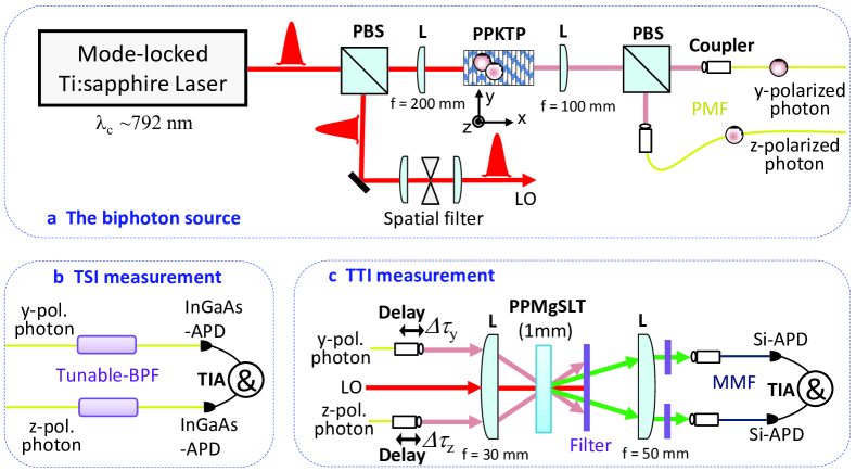
Figure 4: Experimental setup. (a) shows how biphotons were generated; (b) measurement system for two-photon spectral intensity (TSI); (c) measurement system fortwo-photon temporal intensity (TTI). L, lens; PBS, polarizing beam splitter; PMF, polarization maintaining fiber; BPF, bandpass filters; APD, avalanche photodiode; LO, local oscillator; TIA, time-interval analyzer; &, coincidence counter.

The temporal width of the LO pulse was estimated to be approximately 0.12 ps from the bandwidth of the pump pulse. The group-velocity difference between the LO pulse and the photons passing through the PPMgSLT was calculated to be 0.22 ps. We therefore estimated the temporal resolution for a one-photon detection with Si-APD to be $0.12+0.22=0.34$ ps, and for a two-photon detection, $0.34\times\sqrt{2}\approx 0.48$ ps.

Pump pulse spectra for 2.8-nm and 8.1-nm bandwidths In our experiment, the femtosecond laser pulse had a Gaussian distribution with a center wavelength of 792 nm and bandwidth of 8.1 nm, as shown in Fig. 5 (red curve). This spectrum was used for the TSIs and TTIs in Figs. 2b and c in the main text. After the insertion of a bandpass filter, the bandwidth became 2.8 nm, while the center wavelength was unchanged, as shown in Fig. 5 (blue curve). This spectrum was used for the results in Fig. 2a in the main text.

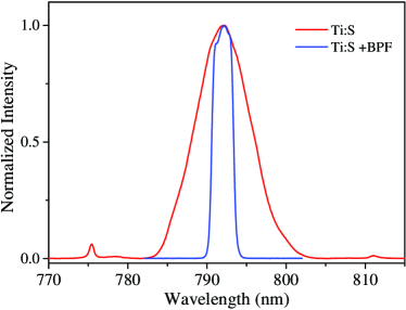
Figure 5: Pump spectra: (a) red the original spectrum from the mode-locked titanium sapphire laser; (b) blue the spectrum after the insertion of a BPF.

Coordinates and parameters We summarize the coordinates and parameters used in this paper, as shown in Figs. 6(a-f). $\Delta\nu_{y}$, $\Delta\nu_{z}$, $\nu_{+}$ and $\nu_{-}$ are the horizontal, vertical, diagonal and anti-diagonal axes respectively in the frequency domain; $\Delta\tau_{y}$, $\Delta\tau_{z}$, $\tau_{+}$ and $\tau_{-}$ are the horizontal, vertical, diagonal and anti-diagonal axes, respectively, in the time domain; $\delta\nu_{yc}$ is the FWHM for the distribution long cross section of $\Delta\nu_{z}=0$; meanwhile, $\delta\nu_{y}$, $\delta\nu_{+}$ and $\delta\nu_{-}$ are the FWHM for the marginal distribution by projecting the data onto the axes of $\Delta\nu_{y}$, $\nu_{+}$ and $\nu_{-}$ respectively. Finally, $\delta\tau_{yc}$ is the FWHM for the distribution along the cross section of $\Delta\tau_{z}=0$; and $\delta\tau_{y}$, $\delta\tau_{+}$ and $\delta\tau_{-}$ are the FWHM for the marginal distribution by projecting the data onto the axes of $\Delta\tau_{y}$, $\tau_{+}$ and $\tau_{-}$ respectively.

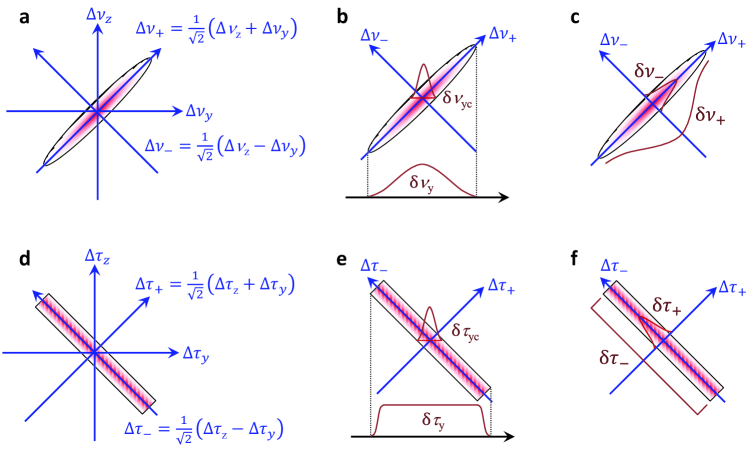
Figure 6: Coordinates and parameters. (a) The coordinate for the frequency domain; (b) $\delta\nu_{yc}$ is the FWHM of the distribution along the $\Delta\nu_{y}$ direction; $\delta\nu_{y}$ is the FWHM of the projected distribution onto the $\Delta\nu_{y}$ direction; (c) $\delta\nu_{+}$ is the FWHM of the projected distribution onto the $\nu_{+}$ direction; $\delta\nu_{-}$ is the FWHM of the projected distribution onto the $\nu_{-}$ direction; (d) the coordinate for the time domain; (e) $\delta\tau_{yc}$ is the FWHM of the distribution along the $\Delta\tau_{y}$ direction; $\delta\tau_{y}$ is the FWHM of the projected distribution onto the $\Delta\tau_{y}$ direction; (f) $\delta\tau_{+}$ is the FWHM of the projected distribution onto the $\tau_{+}$ direction; $\delta\tau_{-}$ is the FWHM of the projected distribution onto the $\tau_{-}$ direction.

Reproduction of the TSIs and TTIs We take Fig. 2b in the main text as an example to show the details of the experimental data processing method. The image on the left in Fig. 2b is the density plot of the TSI, which was scanned along the $\Delta\nu_{y}$ direction at each $\Delta\nu_{z}$ value. Figure 7a is the waterfall plot of Fig. 2b. We fitted the distributions along the $\Delta\nu_{z}$ direction using Gaussian functions, and obtained an averaged FWHM value of $\delta\nu_{yc}=0.21$ THz. Next, we projected the TSI data onto the axis of $\Delta\nu_{y}$, and obtained the marginal distribution, shown in Fig. 3b. The FWHM value of $\delta\nu_{y}=1.9$ THz was estimated with a Gaussian function.

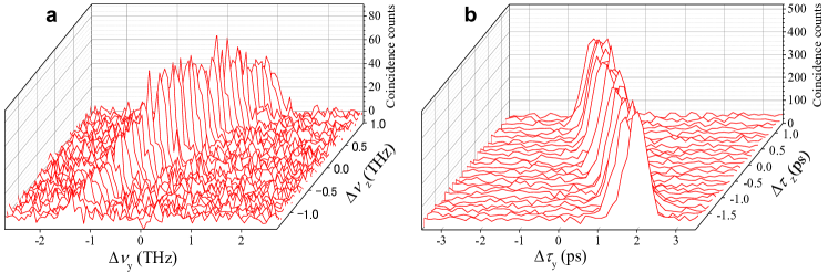
Figure 7: Detailed analysis of the TSI and TTI. (a) The waterfall plots of the TSI; and (b) TTI in Fig. 2b.

Similar results can also be obtained for the temporal data. The density plot of the TTI in Fig. 2b was scanned by 76$\times$76 steps. Figure 7b is the waterfall plot of the TTI. We fitted the distributions along the $\Delta\tau_{z}$ direction using Gaussian functions, and obtained a FWHM of $\delta\tau_{yc}=0.26$ ps. From the projection of the TTI onto the $\Delta\tau_{y}$ axis, we obtained the marginal distribution, as shown in Fig. 3b. With a rectangular-like profile, we estimated a FWHM value of $\delta\tau_{y}=4.3$ ps. The other four data measurements in Figs. 2a and c were processed similarly. Using all the FWHM values, we reproduced the TSIs and TTIs in Fig. 2. We summarize the parameters for TSI and TTI in Table  2.

			Measured				Reproduced
Width			$\delta\nu_{y}$	$\delta\nu_{yc}$	$\delta\tau_{y}$	$\delta\tau_{yc}$	$\delta\nu_{+}$	$\delta\nu_{-}$	$\delta\tau_{+}$	$\delta\tau_{-}$
Unit			(THz)	(THz)	(ps)	(ps)	(THz)	(THz)	(ps)	(ps)
a	$\Delta\lambda_{p}$=2.8 nm	$L$=30 mm	0.82	0.19	4.2	0.54	1.2	0.13	0.38	5.9
b	$\Delta\lambda_{p}$=8.1 nm	$L$=30 mm	1.9	0.21	4.3	0.26	2.7	0.14	0.18	6.1
c	$\Delta\lambda_{p}$=8.1 nm	$L$=10 mm	1.7	0.49	1.3	0.25	2.3	0.33	0.18	1.8

Table 2: The parameters for TSI and TTI. Summary of the bandwidths for measured and reproduced TSI/TTI.

Measurement of TSI The TSI was measured using two center-wavelength-tunable BPFs, which had a Gaussian-shaped filter function with an FWHM of 0.56 nm and a tunable central wavelength from 1560-1620 nm Shimizu and Edamatsu (2009); Jin et al. (2013); Bisht and Shimizu (2015). The two single photon detectors used in this measurement were two InGaAs avalanche photodiode (APD) detectors (ID210, idQuantique), which had a quantum efficiency of around 20%, with a dark count of around 2 kHz. To measure the TSI of the photon pairs, we scanned the central wavelength of the two BPFs, and recorded the coincidence counts. The two BPFs were moved 0.1-nm per step and 60$\times$60 steps in all. The coincidence counts were accumulated for 5 s for each point.

Supplementary Information

S1: Theoretical model of TSI and TTI For a deepper understanding of this experiment, we constructed a simple but effective mathematical model for the biphotons from the PPKTP crystal. The two-photon spectral amplitude (TSA), $f(\nu_{s},\nu_{i})$, is the product of the pump-envelope function and phase-matching function. For simplicity in the calculation, we define $\nu_{s}\equiv\Delta\nu_{y}$ and $\nu_{i}\equiv\Delta\nu_{y}$ as the shifted-frequencies of the signal and idler photons in the main text. Without loss of generality, we assume the pump-envelope function as $\alpha(\nu_{s}+\nu_{i})=\exp[-a(\nu_{s}+\nu_{i})^{2}]$, where $a$ is determined by the spectral width of the pump laser. $\alpha(\nu_{s}+\nu_{i})$ has a distribution 135-degrees to the horizontal axis (i.e., it is distributed along the anti-diagonal direction, as shown in Fig. 8a). The phase-matching function is $\Phi(\omega_{s},\omega_{i})={\rm sinc}[b(\nu_{s}-\nu_{i})]$, where $b$ is determined by the length of the PPKTP crystal. The PPKTP crystal satisfies the GVM condition at telecom wavelength Jin et al. (2013); König and Wong (2004); Evans et al. (2010); Gerrits et al. (2011); Eckstein et al. (2011) , therefore, its phase-matching function has a distribution 45-degrees to the horizontal axis (i.e., distributed along the diagonal direction, as shown in Fig. 8b). The TSA can be written as $f(\nu_{s},\nu_{i})=\exp[-a(\nu_{s}+\nu_{i})^{2}]{\rm sinc}[b(\nu_{s}-\nu_{i})]$, which is the product of the pump-envelope function and phase-matching function. In this experiment, the pump envelope is wider than the width of the phase-matching function; therefore, their product also distributes along the diagonal direction. That is, the signal and idler are positively correlated, as shown in Fig. 8c. The two-photon spectral intensity is $|f(\nu_{s},\nu_{i})|^{2}$, as shown in Fig. 8d.

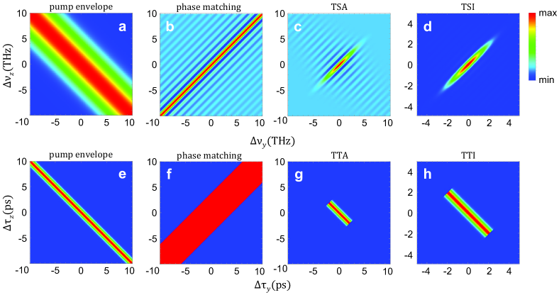
Figure 8: The mathematical model. The first row is for spectral distribution: (a) pump envelope function $\exp[-a(\nu_{s}+\nu_{i})^{2}]$; (b) phase matching function ${\rm sinc}[b(\nu_{s}-\nu_{i})]$; (c) two-photon spectral amplitude (TSA) $f(\nu_{s},\nu_{i})$; (d) two-photon spectral intensity (TSI) $|f(\nu_{s},\nu_{i})|^{2}$. The second row shows the corresponding temporal distributions: (e) temporal pump envelope function $\exp[-\frac{(t_{s}+t_{i})^{2}}{16a}]$; (f) temporal phase matching function ${\rm rect}(\frac{t_{s}-t_{i}}{2b})$; (g) two-photon temporal amplitude (TTA) $F(t_{s},t_{i})$; (h) two-photon temporal intensity (TTI) $|F(t_{s},t_{i})|^{2}$. The parameters are set at $a=0.04$ and $b=4$ for all the figures.

After the long calculation described in S2, the Fourier transform of $f(\nu_{s},\nu_{i})$ can be analytically obtained as $F(t_{s},t_{i})=c_{0}\exp[-\frac{(t_{s}+t_{i})^{2}}{16a}]{\rm rect}(\frac{t_{s}-t_{i}}{2b})$, where $c_{0}=\frac{2\pi^{3}\sqrt{\pi}}{b\sqrt{a}}$. Note that we define $t_{s}\equiv\Delta\tau_{y}$ and $t_{i}\equiv\Delta\tau_{z}$ as the shifted-time for the signal and idler photons in the main text. Here, $\exp[-\frac{(t_{s}+t_{i})^{2}}{16a}]$ is the pump-envelope function in the time domain; ${\rm rect}(\frac{t_{s}-t_{i}}{2b})$ is the phase-matching function in the time domain; $F(t_{s},t_{i})$ is the two-photon temporal amplitude (TSA) and $|F(t_{s},t_{i})|^{2}$ is just the two-photon temporal intensity (TTI). The distribution of these functions is shown in Figs. 8e - h. It is interesting to note that, $\nu_{s}$ and $\nu_{i}$ can not be written in a separated form in $f(\nu_{s},\nu_{i})$. However, if we introduce new variables $\nu_{\pm}=\frac{1}{{\sqrt{2}}}(\nu_{s}\pm\nu_{i})$, $\nu_{+}$ and $\nu_{-}$ can be separated in $f(\nu_{+},\nu_{-})$. The situation is similar for $\tau_{s}$ and $\tau_{i}$, as explained in Eq. (3) in the main text. Another interesting feature is that the pump-envelope and phase-matching functions are independent from each other in both the spectral and temporal domains. The spectral and temporal phase-matching functions are varied simultaneously by changing the parameter a, while phase-matching functions are not affected. Similar phenomena can be observed for the spectral and temporal pump-envelope functions by changing the parameter b: varying the $sinc$ function in the spectral domain corresponds to varying the $rect$ function in the time domain, while the Gaussian-shaped spectral and temporal pump-envelope functions are not affected.

This model is used for the simulations of Fig. 2 in the main text. For Fig. 2a, we changed the pump-envelope function from a Gaussian function to a convolution between a Gaussian function and rectangular function, because the pump laser for Fig. 2a was filtered by a near-rectangular shaped BPF.

S2: Theoretical calculation of TTA from TSA

For a pump-envelope function $\exp[-a(\nu_{s}+\nu_{i})^{2}]$ and a phase-matching function ${\rm sinc}[b(\nu_{s}-\nu_{i})]$, the two-photon spectral amplitude (TSA) can be written as

$$f(\nu_{s},\nu_{i})=\exp[-a(\nu_{s}+\nu_{i})^{2}]{\rm sinc}[b(\nu_{s}-\nu_{i})]$$ (4)

The two-photon temporal amplitude (TTA) is the Fourier transform ($\mathscr{F}$) of $f(\nu_{s},\nu_{i})$, and can be calculated as follows.

$$\begin{array}[]{lll}\mathscr{F}\{f(\nu_{s},\nu_{i})\}&=&\mathscr{F}\{\exp[-a(\nu_{s}+\nu_{2})^{2}]{\rm sinc}[b(\nu_{s}-\nu_{2})]\}\\ \\ &=&\mathscr{F}\{\exp[-a(\nu_{s}+\nu_{i})^{2}]\}\otimes\mathscr{F}\{{\rm sinc}[b(\nu_{s}-\nu_{i})]\}\\ \\ &=&[2\pi\sqrt{\frac{\pi}{a}}\exp(-\frac{{t_{s}^{2}}}{{4a}})\delta(t_{s}-t_{i})]\otimes[2\pi^{2}\frac{1}{b}{\rm rect}(\frac{{t_{s}}}{b})\delta(t_{s}+t_{i})]\\ \\ &=&\int_{-\infty}^{\infty}{\int_{-\infty}^{\infty}{d\tau_{s}d\tau_{i}[}}2\pi\sqrt{\frac{\pi}{a}}\exp(-\frac{{\tau_{s}^{2}}}{{4a}})\delta(\tau_{s}-\tau_{i})][2\pi^{2}\frac{1}{b}{\rm rect}(\frac{{t_{s}-\tau_{s}}}{b})\delta(t_{s}+t_{i}-\tau_{s}-\tau_{i})]\\ \\ &=&\int_{-\infty}^{\infty}{d\tau_{s}[}2\pi\sqrt{\frac{\pi}{a}}\exp(-\frac{{\tau_{s}^{2}}}{{4a}})][2\pi^{2}\frac{1}{b}{\rm rect}(\frac{{t_{s}-\tau_{s}}}{b})\delta(t_{s}+t_{i}-\tau_{s}-\tau_{s})]\\ \\ &=&\int_{-\infty}^{\infty}{d\tau_{s}[}2\pi\sqrt{\frac{\pi}{a}}\exp({-\frac{{\tau_{s}^{2}}}{{4a}}})][2\pi^{2}\frac{1}{b}{\rm rect}(\frac{{t_{s}-\tau_{s}}}{b})\frac{1}{2}\delta(\tau_{s}-\frac{{t_{s}+t_{i}}}{2})]\\ \\ &=&\frac{{2\pi^{3}}}{b}\sqrt{\frac{\pi}{a}}\exp[-\frac{{(t_{s}+t_{i})^{2}}}{{16a}}]{\rm rect}(\frac{{t_{s}-t_{i}}}{{2b}})\\ \\ &=&c_{0}\exp[-\frac{{(t_{s}+t_{i})^{2}}}{{16a}}]{\rm rect}(\frac{{t_{s}-t_{i}}}{{2b}}),\\ \\ \end{array}$$ (5)

where $\otimes$ is the convolution symbol and $c_{0}=\frac{{2\pi^{3}\sqrt{\pi}}}{{b\sqrt{a}}}$. In conclusion, the TTA ($F(t_{s},t_{i})$) can be calculated from the Fourier transform of TSA ($f(\nu_{s},\nu_{i})$) with the following form:

$$F(t_{s},t_{i})=\mathscr{F}\{f(\nu_{s},\nu_{i})\}=c_{0}\exp[-\frac{{(t_{s}+t_{i})^{2}}}{{16a}}]{\rm rect}(\frac{t_{s}-t_{i}}{2b}).$$ (6)

References

- Stark (1982) Henry Stark, Applications of optical Fourier transforms (Academic Press, 1982).
- Goodman (2017) Joseph W. Goodman, Introduction to Fourier Optics, 4th ed. (Freeman, W. H., 2017).
- Zhang et al. (2014) Chi Zhang, Xiaoming Wei, Michel E. Marhic, and Kenneth K. Y. Wong, “Ultrafast and versatile spectroscopy by temporal fourier transform,” Sci. Rep. 4, 5351 (2014).
- Smith (2011) Brian C. Smith, Fundamentals of Fourier Transform Infrared Spectroscopy, 2nd ed. (CRC Press, 2011).
- Bell (1972) Robert Bell, Introductory Fourier Transform Spectroscopy, 1st ed. (Academic Press, 1972).
- Sirohi (2017) Rajpal Sirohi, Optical Methods of Measurement: Whole field Techniques, 2nd ed. (CRC Press, 2017).
- Griffiths and De Haseth (2007) Peter R. Griffiths and James A. De Haseth, Fourier Transform Infrared Spectrometry, 2nd ed. (Wiley-Interscience, 2007).
- VanderLugt (2005) Anthony VanderLugt, Optical Signal Processing (Wiley-Interscience, 2005).
- Rhodes (2009) W.T. Rhodes, Fourier Optics and Optical Signal Processing (Wiley-Blackwell, 2009).
- Chan et al. (2011) Han-Sung Chan, Zhi-Ming Hsieh, Wei-Hong Liang, A. H. Kung, Chao-Kuei Lee, Chien-Jen Lai, Ru-Pin Pan, and Lung-Han Peng, “Synthesis and measurement of ultrafast waveforms from five discrete optical harmonics,” Science 331, 1165 (2011).
- Suhaimi et al. (2015) Nurul Sheeda Suhaimi, Chiaki Ohae, Trivikramarao Gavara, Kenichi Nakagawa, Feng-Lei Hong, and Masayuki Katsuragawa, “Generation of five phase-locked harmonics by implementing a divide-by-three optical frequency divider,” Opt. Lett. 40, 5802–5805 (2015).
- Kocsis et al. (2011) Sacha Kocsis, Boris Braverman, Sylvain Ravets, Martin J. Stevens, Richard P. Mirin, L. Krister Shalm, and Aephraim M. Steinberg, “Observing the average trajectories of single photons in a two-slit interferometer,” Science 332, 1170 (2011).
- Aspden et al. (2016) Reuben S. Aspden, Miles J. Padgett, and Gabriel C. Spalding, “Video recording true single-photon double-slit interference,” American Journal of Physics, Am. J. Phys. 84, 671–677 (2016).
- Eckstein et al. (2011) Andreas Eckstein, Andreas Christ, Peter J. Mosley, and Christine Silberhorn, “Highly efficient single-pass source of pulsed single-mode twin beams of light,” Phys. Rev. Lett. 106, 013603 (2011).
- Jin et al. (2016) Rui-Bo Jin, Ryosuke Shimizu, Mikio Fujiwara, Masahiro Takeoka, Ryota Wakabayashi, Taro Yamashita, Shigehito Miki, Hirotaka Terai, Thomas Gerrits, and Masahide Sasaki, “Simple method of generating and distributing frequency-entangled qudits,” Quantum Sci. Technol. 1, 015004 (2016).
- Chen et al. (2017) Changchen Chen, Cao Bo, Murphy Yuezhen Niu, Feihu Xu, Zheshen Zhang, Jeffrey H. Shapiro, and Franco N. C. Wong, “Efficient generation and characterization of spectrally factorable biphotons,” Opt. Express 25, 7300–7312 (2017).
- Jin et al. (2017) Rui-Bo Jin, Guo-Qun Chen, Hui Jing, Changliang Ren, Pei Zhao, Ryosuke Shimizu, and Pei-Xiang Lu, “Monotonic quantum-to-classical transition enabled by positively correlated biphotons,” Phys. Rev. A 95, 062341 (2017).
- Burnham and Weinberg (1970) David C. Burnham and Donald L. Weinberg, “Observation of simultaneity in parametric production of optical photon pairs,” Phys. Rev. Lett. 25, 84–87 (1970).
- Hong et al. (1987) C. K. Hong, Z. Y. Ou, and L. Mandel, “Measurement of subpicosecond time intervals between two photons by interference,” Phys. Rev. Lett. 59, 2044–2046 (1987).
- Larchuk et al. (1993) T. S. Larchuk, R. A. Campos, J. G. Rarity, P. R. Tapster, E. Jakeman, B. E. A. Saleh, and M. C. Teich, “Interfering entangled photons of different colors,” Phys. Rev. Lett. 70, 1603–1606 (1993).
- Shih et al. (1994) Y. H. Shih, A. V. Sergienko, M. H. Rubin, T. E. Kiess, and C. O. Alley, “Two-photon interference in a standard mach-zehnder interferometer,” Phys. Rev. A 49, 4243–4246 (1994).
- Giovannetti et al. (2002) Vittorio Giovannetti, Lorenzo Maccone, Jeffrey H. Shapiro, and Franco N. C. Wong, “Generating entangled two-photon states with coincident frequencies,” Phys. Rev. Lett. 88, 183602 (2002).
- Jin and Shimizu (2018) Rui-Bo Jin and Ryosuke Shimizu, “Extended Wiener-Khinchin theorem for quantum spectral analysis,” Optica 5, 93–98 (2018).
- Kim and Grice (2005) Yoon-Ho Kim and Warren P. Grice, “easurement of the spectral properties of the two-photon state generated via type II spontaneous parametric downconversion,” Optics Letters, Opt. Lett. 30, 908–910 (2005).
- Shimizu and Edamatsu (2009) Ryosuke Shimizu and Keiichi Edamatsu, “High-flux and broadband biphoton sources with controlled frequency entanglement,” Opt. Express 17, 16385–16393 (2009).
- Avenhaus et al. (2009) Malte Avenhaus, Andreas Eckstein, Peter J. Mosley, and Christine Silberhorn, “Fiber-assisted single-photon spectrograph,” Opt. Lett. 34, 2873–2875 (2009).
- Fang et al. (2014) Bin Fang, Offir Cohen, Marco Liscidini, John E. Sipe, and Virginia O. Lorenz, “Fast and highly resolved capture of the joint spectral density of photon pairs,” Optica 1, 281 (2014).
- Allgaier et al. (2017) Markus Allgaier, Gesche Vigh, Vahid Ansari, Christof Eigner, Viktor Quiring, Raimund Ricken, Benjamin Brecht, and Christine Silberhorn, “Fast time-domain measurements on telecom single photons,” arXiv:1702.03240 (2017).
- Kuzucu et al. (2008a) Onur Kuzucu, Franco N. C. Wong, Sunao Kurimura, and Sergey Tovstonog, “Joint temporal density measurements for two-photon state characterization,” Phys. Rev. Lett. 101, 153602 (2008a).
- Cho et al. (2014) Young-Wook Cho, Kwang-Kyoon Park, Jong-Chan Lee, and Yoon-Ho Kim, “Engineering frequency-time quantum correlation of narrow-band biphotons from cold atoms,” Phys. Rev. Lett. 113, 063602 (2014).
- König and Wong (2004) Friedrich König and Franco N. C. Wong, “Extended phase matching of second-harmonic generation in periodically poled KTiOPO4 with zero group-velocity mismatch,” Appl. Phys. Lett. 84, 1644 (2004).
- Jin et al. (2013) Rui-Bo Jin, Ryosuke Shimizu, Kentaro Wakui, Hugo Benichi, and Masahide Sasaki, “Widely tunable single photon source with high purity at telecom wavelength,” Opt. Express 21, 10659–10666 (2013).
- Kuzucu et al. (2008b) Onur Kuzucu, Franco N. C. Wong, Sunao Kurimura, and Sergey Tovstonog, “Time-resolved single-photon detection by femtosecond upconversion,” Opt. Lett. 33, 2257–2259 (2008b).
- Nielsen and Chuang (2000) Michael A. Nielsen and Isaac L. Chuang, Quantum Computation and Quantum Information (Cambridge University Press, 2000).
- Schweigler et al. (2017) Thomas Schweigler, Valentin Kasper, Sebastian Erne, Igor Mazets, Bernhard Rauer, Federica Cataldini, Tim Langen, Thomas Gasenzer, Jürgen Berges, and Jörg Schmiedmayer, “Experimental characterization of a quantum many-body system via higher-order correlations,” Nature 545, 323–326 (2017).
- Bisht and Shimizu (2015) Nandan S. Bisht and Ryosuke Shimizu, “Spectral properties of broadband biphotons generated from PPMgSLT under a type-II phase-matching condition,” J. Opt. Soc. Am. B 32, 550–554 (2015).
- Evans et al. (2010) P. G. Evans, R. S. Bennink, W. P. Grice, T. S. Humble, and J. Schaake, “Bright source of spectrally uncorrelated polarization-entangled photons with nearly single-mode emission,” Phys. Rev. Lett. 105, 253601 (2010).
- Gerrits et al. (2011) Thomas Gerrits, Martin J. Stevens, Burm Baek, Brice Calkins, Adriana Lita, Scott Glancy, Emanuel Knill, Sae Woo Nam, Richard P. Mirin, Robert H. Hadfield, Ryan S. Bennink, Warren P. Grice, Sander Dorenbos, Tony Zijlstra, Teun Klapwijk, and Val Zwiller, “Generation of degenerate, factorizable, pulsed squeezed light at telecom wavelengths,” Opt. Express 19, 24434–24447 (2011).