Soliton solutions to the fifth-order Korteweg–de Vries equation
and their applications to surface and internal water waves

Abstract

We study solitary wave solutions of the fifth-order Korteweg–de Vries equation which contains, besides the traditional quadratic nonlinearity and third-order dispersion, additional terms including cubic nonlinearity and fifth-order linear dispersion, as well as two nonlinear dispersive terms. An exact solitary wave solution to this equation is derived and the dependence of its amplitude, width and speed on the parameters of the governing equation are studied. It is shown that the derived solution can represent either an embedded or regular soliton depending on the equation parameters. The nonlinear dispersive terms can drastically influence the existence of solitary waves, their nature (regular or embedded), profile, polarity, and stability with respect to small perturbations. We show, in particular, that in some cases embedded solitons can be stable even with respect to interactions with regular solitons. The results obtained are applicable to surface and internal waves in fluids, as well as to waves in other media (plasma, solid waveguides, elastic media with microstructure, etc.).

I Introduction

The Korteweg–de Vries (KdV) equation

$$\frac{\partial u}{\partial t}+c\frac{\partial u}{\partial x}+\alpha u\frac{\partial u}{\partial x}+\beta\dfrac{\partial^{3}u}{\partial x^{3}}=0,$$ (1)

is the well-known model for the description of weakly-nonlinear long waves in media with small dispersion (see, for instance, Karpman75 ; Whitham74 ; Lamb80 ; Ablowitz81 ; Dodd82 ; Newell85 ). It is widely used in the theory of long internal waves where it describes astonishingly well the main properties of nonlinear waves, even when their amplitudes are not small (see, for instance, the reviews Ostrovsky89 ; Ostrovsky05 ; Apel07 ). This is the simplest model that combines the typical effects of nonlinearity and dispersion, and provides stationary solutions describing both periodic and solitary waves. The KdV equation is completely integrable and possesses many remarkable properties, which can be found in the references cited above.

At the same time, the KdV model cannot provide a detailed description of many important features of nonlinear waves observed in laboratory experiments, such as the non-monotonic dependence of solitary wave speed on amplitude, or the table-top shape of large-amplitude solitary waves Michallet&Barthelemy98 . To capture such properties, the first natural step is a straightforward extension of the KdV model by retaining the next-order nonlinear and dispersive terms in the asymptotic expansion of the solutions to primitive equations, for example the Euler equations with boundary conditions appropriate for oceanographic applications in the case of the ocean gravity waves. A rather general form of the extended KdV equation has been derived by many authors (in application to surface and internal waves as shown in Figure 1 see, e.g., Benney66 ; Lee74 ; Koop81 ; Olver84 ; MarchantSmyth90 ; Lamb96 ; Grimshaw02 ; Giniyatullin14 ; KarRozRut14 ; Karczewska14 ):

$$\frac{\partial u}{\partial t}+\alpha u\frac{\partial u}{\partial x}+\beta\dfrac{\partial^{3}u}{\partial x^{3}}+\varepsilon\left(\alpha_{1}u^{2}\frac{\partial u}{\partial x}+\gamma_{1}u\dfrac{\partial^{3}u}{\partial x^{3}}+\gamma_{2}\frac{\partial u}{\partial x}\dfrac{\partial^{2}u}{\partial x^{2}}+\beta_{1}\dfrac{\partial^{5}u}{\partial x^{5}}\right)=0.$$ (2)

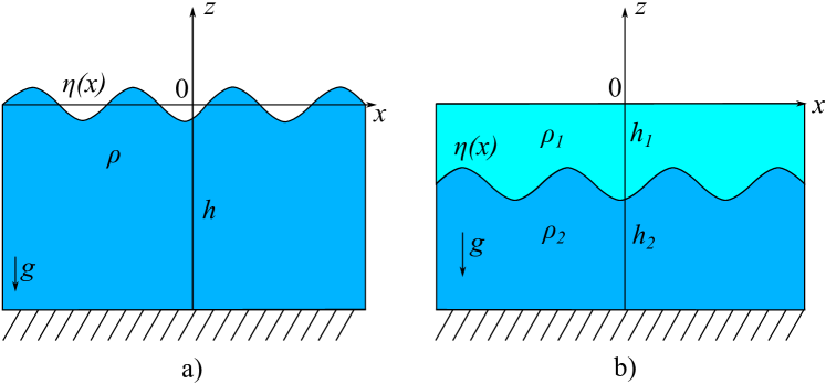
Figure 1: Sketch of two configurations for surface water waves (a) and internal waves in two-layer fluids (b). (Notice that the horizontal and vertical scales are different.)

This equation, written in the coordinate frame moving with the speed $c$, combines the quadratic ($\sim\alpha$) and cubic ($\sim\alpha_{1}$) nonlinear terms, linear dispersion of the 3^rd ($\sim\beta$) and 5^th ($\sim\beta_{1}$) orders, and also higher-order nonlinear dispersion terms with coefficients $\gamma_{1}$ and $\gamma_{2}$; the parameter $\varepsilon\ll 1$ is presumed to be small.

Particular cases of the fifth-order KdV equation, where some coefficients are zero, were also derived for plasma waves Kakutani69 , electromagnetic waves in discrete transmission lines Gorshkov76 , gravity-capillary water waves Abramyan85 ; Hunter88 , waves in a floating ice sheet (see Ref. Guyenne14 and references therein).

In general equation (2) is not integrable, but for particular choices of coefficients it reduces to one of a set of equations that are completely integrable. These are the Gardner equation Slyunyaev99 ; Slyunyaev01 (when $\beta_{1}=\gamma_{1}=\gamma_{2}=0$) or its particular case the standard KdV/mKdV equation (when either $\alpha_{1}=0$ or $\alpha=0$), as well as the Sawada–Kotera and Kaup–Kupershmidt equations (when $\alpha=\beta=0$) Dodd82 ; Newell85 . A comprehensive discussion of equation (2) and its properties can be found in Kichenassamy92 .

The coefficients of equation (2) for surface gravity waves are

$$c=\sqrt{gh},\quad\alpha=\frac{3c}{2h},\quad\alpha_{1}=-\frac{3c}{8h^{2}},\quad\beta=\frac{ch^{2}}{6},\beta_{1}=\frac{19ch^{4}}{360},\quad\gamma_{1}=\frac{5ch}{12},\quad\gamma_{2}=\frac{23ch}{24}.$$ (3)

For the gravity-capillary surface waves, as well as for internal waves in a two-layer fluid, the coefficients are presented in Appendix A. All notations are shown in Figure 1.

Unlike the KdV equation, the higher-order model (2) is not a Hamiltonian equation and does not preserve the energy, in general. However, in the particular cases when it reduces to completely integrable models, it clearly becomes Hamiltonian. Besides those cases, there is one more particular case of $\alpha_{1}=0$ and $\gamma_{2}=2\gamma_{1}$ when equation (2) becomes Hamiltonian, but nonintegrable Champneys97 ; Yang01 . In the meantime, with the help of a near-identity transformation, it can be mapped approximately into one of a number of Hamiltonian equations Kodama85 ; Fokas95 ; FokasLiu96 ; LiZhiSib97 . In particular the asymptotic near-identity transformation

$$\tilde{u}=u+\varepsilon(au^{2}+bu_{xx})$$ (4)

maps equation (2) into itself up to terms of $o(\varepsilon)$, but with the new coefficients

$$\tilde{\alpha_{1}}=\alpha_{1}-a\alpha,\quad\tilde{\beta_{1}}=\beta_{1},\quad\tilde{\gamma_{1}}=\gamma_{1},\tilde{\gamma_{2}}=\gamma_{2}-6a\beta+2b\alpha,$$

where $a$ and $b$ are arbitrary parameters. If we choose the parameters $a=\left(\gamma_{2}-2\gamma_{1}\right)/6\beta$ and $b=0$, then equation (2) can be presented in the Hamiltonian form

$$u_{t}=\frac{\partial}{\partial x}\left(\frac{\delta H}{\delta u}\right),$$ (5)

where the Hamiltonian is $H=\int\mathcal{H}\;\mathrm{d}x$ with the density

$$\mathcal{H}=-\frac{1}{6}\alpha u^{3}+\frac{1}{2}\beta u_{x}^{2}-\varepsilon\left(\frac{1}{12}\tilde{\alpha_{1}}u^{4}+\frac{1}{2}\tilde{\beta_{1}}u_{xx}^{2}-\frac{1}{2}\tilde{\gamma_{1}}uu_{x}^{2}\right).$$ (6)

The Hamiltonian form provides conservation of the “mass” $I_{1}=\int u\;\mathrm{d}x$, “wave energy” $I_{2}=\int\left(u^{2}/2\right)\;\mathrm{d}x$, and Hamiltonian $I_{3}=\int\mathcal{H}\;\mathrm{d}x$. These conserved quantities are very useful in the development of asymptotic methods and perturbation techniques, as well as helping to control the accuracy of numerical schemes. Notice however, as has been shown in Olver84 , the formal Hamiltonians which follow from the approximate evolution equations are not usually the genuine Hamiltonians that can be derived from the primitive equations for small-amplitude wave perturbations and which agree with the physical energy conservation. Even in the classical KdV equation (1) the Hamiltonian does not represent the genuine wave energy. To this end the “correct” KdV equation with the genuine Hamiltonian was derived in Olver84 ; the corresponding equation is a particular case of equation (2) with $\beta_{1}=0$.

If the leading-order evolution equation is integrable, then the underlying physical system is said to be asymptotically integrable up to $O(\varepsilon)$. It turns out that for the higher-order KdV equation (2) with special choices of coefficients, it is possible to extend the asymptotic integrability, even up to $O(\varepsilon^{2})$ Kodama85 ; Fokas95 ; FokasLiu96 . Indeed, the generic KdV equation is asymptotically reducible to the integrable equation by the nonlocal near-identity transformation

$$\tilde{u}=u+\varepsilon\left(a_{1}u^{2}+b_{1}u_{xx}+c_{1}u_{x}\int_{x_{0}}^{x}u\;\mathrm{d}\tilde{x}+d_{1}xu_{t}\right),$$ (7)

where $a_{1}$, $b_{1}$, $c_{1}$, $d_{1}$ are arbitrary constants. This transformation can reduce (2) either to the next member of the KdV hierarchy, or even to the classical KdV equation, with accuracy up to $O(\varepsilon^{2})$. In particular, to transfer equation (2) to the KdV equation one should choose coefficients in (7) of the form

$$a_{1}=\frac{-18\beta^{2}\alpha_{1}+2\alpha^{2}\beta_{1}+3\alpha\beta\gamma_{1}}{9\alpha\beta^{2}}, b_{1}=\frac{-6\beta^{2}\alpha_{1}-\alpha^{2}\beta_{1}+\alpha\beta\gamma_{2}}{2\alpha^{2}\beta},$$

$$c_{1}=\frac{4\alpha\beta_{1}-2\beta\gamma_{1}}{9\beta^{2}}, d_{1}=-\frac{\beta_{1}}{3\beta^{2}}.$$

There are numerous other near-identity transformations; some of them are of special interest because they do not contain a secular term $\sim d_{1}$ as in the formula (7). In particular, the appropriately modified near-identity transformations reducing the higher-order KdV equation to the KdV equation have been successfully used to obtain particular solutions for the higher-order KdV equation from the known solutions of the KdV equation (e.g., the two-soliton solution extending the relevant KdV solution Kraenkel98 ; MarchantSmyth96 ; Marchant99 and the undular bore solution MarchantSmyth2006 ).

In some particular cases when equation (2) is non-integrable it possesses, nevertheless, stationary solitary-type solutions, which can be constructed either numerically or sometimes even analytically. One of the best known cases is the Kawahara equation which follows from equation (2) when $\alpha_{1}=\gamma_{1}=\gamma_{2}=0$ Kawahara72 . This equation contains a rich family of solitary solutions including solitons with monotonic Yamamoto81 and oscillatory tails Kawahara72 ; Gorshkov76 ; Gorshkov79 .

Recently one more particular case of equation (2) was considered, the so–called Gardner–Kawahara equation Giniyatullin14 ; Kurkina15 , when only the nonlinear dispersive terms are absent ($\gamma_{1}=\gamma_{2}=0$). Such a situation may occur, for example, in a two-layer fluid with surface tension between the layers. Solitary solutions for that equation were constructed numerically Kurkina15 and it was shown that among them there are “fat solitons”, similar to those seen in the Gardner equation, and solitons with oscillatory tails, such as in the Kawahara equation, as well as their combination – fat solitons with oscillatory tails.

An analytical solitary wave solution of the non-integrable equation (2) was found in Karczewska14 for a special set of coefficients, when it is not reduced to the Sawada–Kotera or Kaup–Kupershmidt equations. The obtained solution does not contain any free parameters and represents an example of a so-called “embedded soliton”. Embedded solitons co-exist with linear waves propagating with the same speed (they are “embedded” into the continuous spectrum of linear waves, whereas regular solitons can be called “gap” solitons, because they exist when the soliton speed belongs to a gap in the phase speed spectrum of a corresponding linearized system YMKC01 ). The term “embedded soliton” was introduced in Ref. Yang99 , although such solitons were known since 1974 when the first analytical example was obtained in Ref. Nishikawa74 and their stability was proven numerically in Ref. Gorshkov83 (some information about that can be found also in Ref. Petviashvili92 ). As currently known Yang10 , embedded solitons can be both stable and unstable with respect to perturbations of small or even big amplitudes depending on the particular governing equation or set of equations.

Nevertheless, the general problem of existence of solitary wave solutions of equation (2) with arbitrary coefficients remains open so far, and this circumstance motivated our study. Besides the pure academic interest the problem is also topical in application to surface and internal waves of large amplitude in the ocean. Equation (2) can be considered as the model equation capable of describing typical features of large-amplitude solitary waves with good accuracy (see, e.g., Michallet&Barthelemy98 where it was shown that even its reduced version, the Gardner equation, provides solutions similar to those which can be constructed within the fully nonlinear Euler equations). We study the role of higher-order nonlinear dispersive terms ($\sim\gamma_{1},\gamma_{2}$) and their influence on the shape and polarity of solitary wave solutions. By means of the Petviashvili numerical method Petviashvili92 ; Pelinovsky04 we construct stationary solutions of equation (2) and categorise them in terms of dimensionless parameters. We then numerically model non-stationary solutions using a pseudospectral scheme similar to that used in Grimshaw08 ; Alias13 ; Alias14 ; Khusnutdinova17 . We show that these solutions demonstrate soliton-like properties in the course of their interaction with only minor inelastic effect. We also found an exact analytical solution to this equation in the general case without a restriction on its coefficients. The solution represents either the embedded or a regular (gap) soliton, depending on parameters.

II Dimensionless form of the fifth-order KdV equation and its general properties

To minimise the number of parameters in the problem let us present equation (2) in dimensionless form using the change of variables

$$\tau=\frac{s\alpha^{3}t}{\varepsilon\alpha_{1}}\sqrt{\frac{s}{\varepsilon\alpha_{1}\beta}},\quad\xi=\alpha x\sqrt{\frac{s}{\varepsilon\alpha_{1}\beta}},\quad\upsilon=\frac{\varepsilon\alpha_{1}}{\alpha}su,$$ (8)

where $s=\mathrm{sign}\left(\alpha_{1}\beta\right)$ i.e. $s=1$ if $\alpha_{1}\beta>0$, and $s=-1$ if $\alpha_{1}\beta<0$. After that the main equation (2) can be presented in the divergent form:

$$\frac{\partial\upsilon}{\partial\tau}+\frac{\partial}{\partial\xi}\left[\frac{\upsilon^{2}}{2}+s\frac{\upsilon^{3}}{3}+\dfrac{\partial^{2}\upsilon}{\partial\xi^{2}}+B\dfrac{\partial^{4}\upsilon}{\partial\xi^{4}}+\frac{G_{1}}{2}\dfrac{\partial^{2}\upsilon^{2}}{\partial\xi^{2}}+\frac{G_{2}-3G_{1}}{2}\left(\frac{\partial\upsilon}{\partial\xi}\right)^{2}\right]=0,$$ (9)

where

$$B=\alpha^{2}\frac{s}{\alpha_{1}\beta}\frac{\beta_{1}}{\beta},\quad G_{1}=\frac{s}{\alpha_{1}\beta}\alpha\gamma_{1},\quad G_{2}=\frac{s}{\alpha_{1}\beta}\alpha\gamma_{2},$$ (10)

(notice that $s/(\alpha_{1}\beta)>0$). The divergent form immediately provides the “mass conservation” integral $I_{1}$ as defined before. Multiplying this equation by $\upsilon$ and integrating either over the entire axis $\xi$ for solitary waves or over a period for periodic waves, we derive the “energy balance equation”

$$\frac{\partial I_{2}}{\partial\tau}\equiv\frac{\partial}{\partial\tau}\int\frac{\upsilon^{2}}{2}\;\mathrm{d}\xi=\left(G_{1}-\frac{G_{2}}{2}\right)\int\left(\frac{\partial\upsilon}{\partial\xi}\right)^{3}\;\mathrm{d}\xi.$$ (11)

This relationship denotes a distinguishing feature of the model (9) which describes, in general, either time decay or growth of “wave energy” $I_{2}$ due to the presence of the nonlinear dispersive terms. Such conditionally defined “wave energy” is conserved either in the trivial case when $G_{1}=G_{2}=0$ or in the special case when $G_{2}=2G_{1}$ Champneys97 . For stationary waves described by even functions $\upsilon(\xi)$, the right-hand side of equation (11) is zero, and their “energy” is also conserved for any values of $G_{1}$ and $G_{2}$. (Note that in the case of surface gravity waves, $G_{1}-G_{2}/2=-3/2$.)

For waves of infinitesimal amplitude, $\upsilon\rightarrow 0$, equation (9) can be linearised. Looking for a solution in the form $\upsilon\sim\exp{i\left(\tilde{\omega}\tau-\kappa\xi\right)}$, we obtain the dispersion relation $\tilde{\omega}\left(\kappa\right)$ and phase speed $V_{ph}(\kappa)$, in the coordinate frame moving with speed $c$, of the form

$$\tilde{\omega}=-\kappa^{3}+B\kappa^{5},\quad V_{ph}(\kappa)\equiv\frac{\tilde{\omega}}{\kappa}=-\kappa^{2}+B\kappa^{4}.$$ (12)

The plot of the phase speed is shown in Figure 2 for three typical values of the parameter $B$. Note that for surface water waves $B=57/5>0$, therefore qualitatively the dispersion curve is similar to curve $B=1$. The same is true for oceanic internal waves, as follows from the expressions for the coefficients of (2) (see Appendix A). In some cases for internal waves in laboratory tanks the coefficient $B$ can be zero or negative.

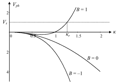
Figure 2: Plots of phase speed as per equation (12) for zero, positive and negative values of parameter $B=0$. The dashed horizontal line illustrates speed $V_{s}$ of a solitary wave, which can generate a small amplitude oscillatory wave at the resonant wavenumber $\kappa_{r}$.

In the case of $B\leq 0$ the phase speed is a monotonic function of $\kappa$, whereas for $B>0$ it has a minimum, $V_{min}=-1/(4B)$, at the point $\kappa_{c}=\left(2B\right)^{-1/2}$ (see Figure 2). The concept of phase speed is very useful in understanding the process of interaction of a moving source (e.g. a solitary wave) with linear waves. In particular, if the speed of a source $V_{s}$ is such that there is no resonance with any linear wave i.e. there is no intersection of the dashed line in Figure 2 with the dispersion curve (e.g. when $V_{s}<V_{\mathrm{min}}$), then the source does not lose energy for the wave excitation. Otherwise, in the case of a resonance (see the intersection of the dashed line with the curve for $B=1$) the source, in general, can experience energy losses for the generation of a linear wave and, as a result, it gradually decelerates. Without external compensation of energy losses, such a source usually cannot move steadily. However, there are several examples of embedded solitons which can steadily propagate with the same speed as a linear wave, but not exciting it effectively. The physics of such a phenomenon has not been well understood yet; it requires further study which is beyond the scope of this paper. Therefore, the no-resonance condition $V_{s}\neq V_{ph}$ can provide only an indication of when a solitary wave can most likely be expected.

III Stationary solutions of the fifth-order KdV equation

Consider now stationary solutions to equation (9) in the form of travelling waves depending only on one variable, $\zeta=\xi-V\tau$, where $V$ is the wave speed. In this case equation (9) can be reduced to an ODE and integrated once (the constant of integration is set to zero for solitary waves):

$$B\dfrac{\mathrm{d}^{4}\upsilon}{\mathrm{d}\zeta^{4}}+\dfrac{\mathrm{d}^{2}\upsilon}{\mathrm{d}\zeta^{2}}-V\upsilon+\frac{\upsilon^{2}}{2}+s\frac{\upsilon^{3}}{3}+\frac{G_{1}}{2}\dfrac{\mathrm{d}^{2}\upsilon^{2}}{\mathrm{d}\zeta^{2}}+\frac{G_{2}-3G_{1}}{2}\left(\frac{\mathrm{d}\upsilon}{\mathrm{d}\zeta}\right)^{2}=0.$$ (13)

There are five independent parameters in this equation: $B$, $G_{1}$, $G_{2}$, $s$, and $V$, which determine the structure of a solitary wave. This equation actually splits into two independent equations with different properties; one equation with negative cubic term ($s=-1$), and another one with positive cubic term ($s=1$). We will derive a particular soliton solution to this equation for both $s=1$ and $s=-1$. The case of $s=0$ with a specific link between the parameters, $G_{2}=2G_{1}$, has been studied in Champneys97 .

As a first step, let us consider solitary wave asymptotics at plus/minus infinity. Assuming that soliton solutions decay at infinity, let us linearise equation (13) (simply omit all nonlinear terms) and seek a solution of the remaining linear equation in the form $\upsilon\sim\exp{\left(\mu\zeta\right)}$. Substituting this trial solution into the linearised equation (13), we obtain an algebraic equation for $\mu$ of the form (cf. Champneys97 ):

$$B\mu^{4}+\mu^{2}-V=0.$$ (14)

The roots of this bi-quadratic equation are

$$\mu_{1,2}=\pm\sqrt{\frac{-1+\sqrt{1+4BV}}{2B}},\quad\mu_{3,4}=\pm\sqrt{\frac{-1-\sqrt{1+4BV}}{2B}}.$$ (15)

Let us analyse the roots in detail (an alternative analysis of the roots in the plane of different parameters can be found in Champneys97 ). Firstly we consider the case when the parameter $B$ is negative. For negative $V$ we have $4BV>0$ and $\sqrt{1+4BV}>1$, therefore the roots $\mu_{1,2}$ are purely imaginary, and the roots $\mu_{3,4}$ are real. Solutions corresponding to purely imaginary roots are not decaying and cannot represent solitary waves with zero amplitude at infinity. If $V=0$, then $\mu_{1,2}=0$ and the corresponding solutions do not decay at infinity.

If $0<V<-1/(4B)$, then we have $\sqrt{1+4BV}>0$, and all four roots $\mu_{1,2,3,4}$ are real. In this case soliton solutions are possible, with exponentially decaying asymptotics at infinity. Finally, if $V>-1/(4B)$, then $\sqrt{1+4BV}$ is complex; all roots are complex-conjugate in pairs $\mu_{1,2}=\pm(p_{1}+iq_{1})$, $\mu_{3,4}=\pm(p_{2}+iq_{2})$. Due to the presence of the real parts of the roots, $p_{1,2}$, there can be soliton solutions with oscillatory asymptotics. The decay rate of a solitary wave in the far field is determined by the root with the smallest value of $|p_{1,2}|$.

Assume now that $B$ is positive. It follows from a similar analysis of roots as was done for negative $B$ that, for $V<V_{min}\equiv-1/(4B)$, solitary waves with oscillatory asymptotics are possible. For $V_{min}<V<0$, the roots are purely imaginary, therefore no solitons with zero asymptotics can exist in this case. For $V>0$ the roots $\mu_{1,2}$ are purely real, then embedded solitons with exponential asymptotics are possible.

In the particular case of $B=0$, equation (14) has two real roots corresponding to soliton solutions, provided that $V>0$. These findings can be summarised with the help of a schematic diagram, as shown in Figure 3.

It should be noted that the analysis of roots only predicts possible asymptotics of solitons provided that they exist, but it does not guarantee their existence. In particular, if $B=0$, then soliton solutions with monotonically decaying exponential asymptotics could exist for any $V>0$ (see case (b) in the diagram), but in fact they exist only for $0<V<1/6$ (see, e.g., Kurkina15 ).

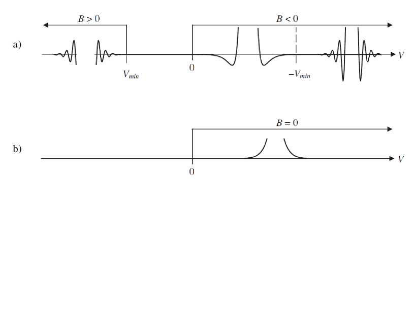
Figure 3: Asymptotics of possible soliton solutions of equation (13) with different signs of parameter $B$ (panel a). Panel (b) shows the asymptotics of regular solitons in the case of $B=0$ or embedded solitons in the case of $B>0$.

III.1 Solitary wave solution of the fifth-order KdV equation

Let us consider a trial solution to (13) in the form of a sech² solitary wave (in a similar way to what was done in Kichenassamy92 ), taking the form

$$\upsilon\left(\zeta\right)=A\mathop{\rm sech}\nolimits^{2}\left(K\zeta\right),$$ (16)

where $A$ is the soliton amplitude and $K$ is the parameter determining its half-width $\Delta=1/K$ (similar solution was constructed in Champneys97 for the particular case of $s=0$ and $G_{2}=2G_{1}$). By substitution of this solution into equation (13) we obtain

$$C_{2}\mathop{\rm sech}\nolimits^{2}\left(K\zeta\right)+C_{4}\mathop{\rm sech}\nolimits^{4}\left(K\zeta\right)+C_{6}\mathop{\rm sech}\nolimits^{6}\left(K\zeta\right)=0,$$ (17)

where

$$C_{2} =16BK^{4}+4K^{2}-V,$$ (18)

$$C_{4} =-120BK^{4}+[2(G_{1}+G_{2})A-6]K^{2}+\frac{A}{2},$$ (19)

$$C_{6} =120BK^{4}+s\frac{A^{2}}{3}-2(G_{2}+2G_{1})AK^{2}$$ (20)

(cf. Kichenassamy92 where a slightly different approach was used). Equating the coefficients $C_{2}$ and $C_{4}$ to zero, we obtain

$$V =4K^{2}\left(1+4BK^{2}\right)=\frac{4\left(\Delta^{2}+4B\right)}{\Delta^{4}},$$ (21)

$$A =12K^{2}\frac{1+20BK^{2}}{1+4\left(G_{1}+G_{2}\right)K^{2}}=\frac{12}{\Delta^{2}}\frac{\Delta^{2}+20B}{\Delta^{2}+4\left(G_{1}+G_{2}\right)}.$$ (22)

Eliminating $A$ from equation (20) with the help of equation (22), we obtain the quadratic equation for $R\equiv K^{2}$ of the form

$$80B\left(G_{1}^{2}+G_{1}G_{2}-10Bs\right)R^{2}+4\left(2G_{1}^{2}+3G_{1}G_{2}+G_{2}^{2}-5BG_{2}-20Bs\right)R-5B+2G_{1}+G_{2}-2s=0.$$

This equation has two roots, in general, and the corresponding expression for the half-width of a solitary wave is determined by

$$\Delta_{1,2}^{2}=\frac{40B\left(G_{1}G_{2}+G_{1}^{2}-10Bs\right)}{5B\left(G_{2}+4s\right)-3G_{1}G_{2}-2G_{1}^{2}-G_{2}^{2}\pm\left(5B-G_{1}-G_{2}\right)\sqrt{\left(2G_{1}+G_{2}\right)^{2}-40Bs}}.$$ (23)

Thus, we see that a solitary wave solution in the form of (16) does exist for a certain set of parameters $B$, $G_{1}$ and $G_{2}$. One of the obvious restrictions on the set of parameters is (we have two expressions as $s$ can be positive or negative)

$$\left(2G_{1}+G_{2}\right)^{2}-40Bs\geq 0\quad\Rightarrow\quad B\geq-\frac{\left(2G_{1}+G_{2}\right)^{2}}{40}\quad\text{for $s=-1$, or}\quad B\leq\frac{\left(2G_{1}+G_{2}\right)^{2}}{40}\quad\text{for $s=1$}\quad.$$ (24)

Below we consider a few particular cases and analyse the corresponding soliton solutions.

III.2 The Gardner–Kawahara equation ($G_{1}=G_{2}=0$)

In this case the expressions for $\Delta$, $V$ and $A$ simplify considerably. The half-width is given by

$$\Delta^{2}=\frac{-40Bs}{2s\pm\sqrt{-10Bs}}.$$ (25)

The soliton derived from (25) can either be an embedded soliton or a regular soliton, dependent upon its speed as defined by (21) and the value of $B$. Due to the presence of $s$ in (25) we consider two sub-cases: $s=-1$ and $s=1$.

III.2.1 The Gardner–Kawahara equation with $s=-1$

In this case the only meaningful solution to (25) is

$$\Delta^{2}=\frac{40B}{-2+\sqrt{10B}},$$ (26)

with $B>2/5$ for a real solution. Then from equation (21) it follows that $V>0$. With $B>0$ the phase speed dependence of linear waves on the wavenumber is shown in Figure 2 by the upper line. Therefore, solution (16) with $V>0$ is the embedded soliton moving in resonance with a linear wave (however gap solitons can co-exist with the embedded soliton as will be shown below). Figure 4 shows the dependence of the soliton parameters on $B$. The soliton amplitude monotonically increases with $B$, whereas its width and speed non-monotonically depend on this parameter. The minimum value $\Delta_{min}=\sqrt{32}$ is attained at $B=8/5$, and maximum speed $V_{max}=5/32$ occurs at $B=128/45$. Soliton profiles for these two cases will be shown below in Figure 9 in comparison with regular solitons, numerically constructed for the same values of $B$. The asymptotics of embedded solitons are in agreement with the prediction from the analysis of roots of the characteristic equation (14) - see Figure 3b.

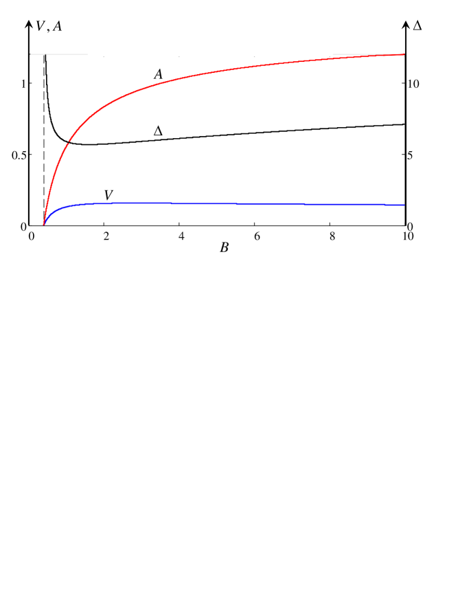
Figure 4: (color online) Dependence of embedded soliton parameters on $B$, for $G_{1}=G_{2}=0$ with $s=-1$. Vertical dashed line shows the limiting value of the parameter $B_{lim}=2/5$, below which the soliton does not exist.

III.2.2 The Gardner–Kawahara equation with $s=1$

In this case the soliton half-width takes the form

$$\Delta^{2}=\frac{-40B}{2\pm\sqrt{-10B}},\quad\text{where $B<0$.}\quad$$ (27)

If the positive sign is taken in front of the square root, then the right-hand side of the expression is positive for all negative $B$, whereas if the negative sign is taken in front of the square root then the expression in the right-hand side is positive only under the restriction $B>-2/5$ (see Figure 5 (a)).

Figure 5: (color online) Dependence of soliton parameters on $B$, for $G_{1}=G_{2}=0$ with $s=1$. Frame a): widths of two different solitons as per equation (27); frame b): speeds of two different solitons as per equation (28); frame c): amplitudes of two different solitons as per equations (29) and (30). Line 1 is for positive sign in these expressions and line 2 for negative signs. Dashed vertical lines correspond to the critical values of parameter $B$: $B=-32/5$ (left line) and $B=-2/5$ (right line). The horizontal dashed line in frame b) shows the limiting value of soliton speed $V_{lim}=-1/10$, when $B\to-\infty$, and the horizontal dashed line in frame c) shows the limiting value of soliton amplitude $A_{lim}=9/4$, when $B\to-\infty$.

Then, from Figure 2 it follows that for $B<0$ the solution (16) represents a regular soliton if $V>0$, and an embedded soliton if $V<0$. The soliton velocity (21) with $\Delta^{2}$ given by equation (27) is

$$V=\frac{4}{\Delta^{4}}\left(\Delta^{2}+4B\right)=-\frac{5B+8\pm 3\sqrt{-10B}}{50B}.$$ (28)

The analysis of this expression shows that, if the positive sign is chosen in front of the square root, then solution (16) represents a regular soliton with $V>0$, if $-32/5<B<0$, and an embedded soliton with $V<0$, if $B<-32/5$. If the sign in front of the square root is negative, then solution (16) represents a regular soliton with $V>0$ within the interval $-2/5<B<0$, whereas beyond this interval soliton solutions do not exist (see Figure 5b).

As follows from equation (22), solitons with positive sign in front of the square root in equation (27) have positive polarity, and solitons with negative sign have negative polarity (see Figure 5c). In particular, when $G_{1}=G_{2}=0$, we have

$$A_{1} =-\frac{360B}{\Delta_{1}^{4}}=-\frac{9}{20B}\left(2-5B+2\sqrt{-10B}\right),$$ (29)

$$A_{2} =-\frac{360}{\Delta_{2}^{4}}=-\frac{9}{20B^{2}}\left(2-5B-2\sqrt{-10B}\right).$$ (30)

Vertical dashed lines in Figure 5 at $B=-2/5$ show the limiting value of this parameter below which the negative polarity solitons cannot exist. Other vertical dashed lines in Figure 5 at $B=-32/5$ show the boundary between the regular solitons with $V>0$ and $B>-32/5$, and embedded solitons with $V<0$ and $B<-32/5$.

The horizontal dashed line in frame b) shows the limiting value of the embedded soliton speed $V_{lim}=-1/10$, when $B\to-\infty$, and the horizontal dashed line in frame c) shows the limiting value of the embedded soliton amplitude $A_{lim}=9/4$, when $B\to-\infty$ (the width of the embedded soliton slowly increases when $B\to-\infty$ as $\Delta\sim 2\sqrt[4]{-10B}$).

Thus, in the interval $-2/5<B<0$, two types of regular solitons can coexist with different widths, speeds, amplitudes, and polarities. When $B<-2/5$ only one soliton of positive polarity can exist which smoothly transfers into the embedded soliton when the parameter $B$ passes through the threshold value $B=-32/5$ where the velocity vanishes. Figure 6 illustrates the profiles of regular solitons of positive and negative amplitudes for three values of $B$ in the indicated interval.

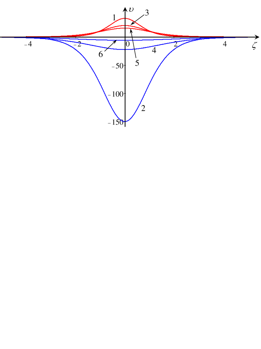
Figure 6: (color online) Profiles of gap solitons of positive and negative polarities for three values of $B$ in the interval $-2/5<B<0$. Specifically $B=-0.05$ for lines 1 and 2, $B=-0.1$ for lines 3 and 4, and $B=-0.15$ for lines 5 and 6.

III.3 A particular case of surface gravity waves ($s=-1$)

Using the expressions for the coefficients of equation (2) for gravity waves (see equation (3)), we obtain the dimensionless parameters $B=57/5$, $G_{1}=10$, $G_{2}=23$ (notice that in this case $G_{2}=2.3G_{1}$, which is very close to the case $G_{2}=2G_{1}$ when the energy is conserved – see equation (11)). For this set of parameters there is only one real root of equation (23)

$$\Delta_{1}=\sqrt{\frac{8436}{\sqrt{2305}-14}}\approx 15.75.$$ (31)

After that we find the amplitude and speed of a soliton in the form

$$A=\frac{3}{148}\left(51-\sqrt{2305}\right)\approx 6.06\cdot 10^{-2},\quad V=\frac{157\sqrt{2305}-89}{390165}\approx 1.91\cdot 10^{-2}.$$ (32)

We see again that $V>0$ and $B>0$, therefore the soliton is in resonance with one of the linear waves as shown in Figure 2 by the upper line. Hence, solution (16) represents again the embedded soliton with exponential asymptotics in agreement with the prediction following from the analysis of roots of characteristic equation (14) - see Figure 3b).

In dimensional variables the amplitude, width and speed of the surface embedded soliton are

$$A_{d}=4hA,\quad\Delta_{d}=h\Delta/6,\quad V_{d}=6V\sqrt{gh},$$

where index $d$ pertains to the dimensional variables, and $h$ is the fluid depth. Setting $h=10$ m, we obtain $A_{d}\approx 2.42\ \text{m}$, $\Delta_{d}\approx 26.25~{}\text{m}$, $V_{d}\approx 1.14\ \text{m/s}$ (the total speed is $c+V_{d}\approx 9.9\ \text{m/s}+1.14\ \text{m/s}\approx 11.04\ \text{m/s}$). Thus, according to this solution, a soliton of small amplitude can exist on the surface of the water. In the meantime, the classical KdV theory predicts the existence of a soliton which has amplitude $A_{e}\approx 5.37\ \text{m}$ and speed $V_{e}\approx 2.66\ \text{m/s}$ at the same width $\Delta_{d}\approx 26.25\ \text{m}$.

The linear wave of infinitesimal amplitude propagating with the same speed as the embedded soliton ($V_{ph}=c+V_{d}$) has dimensional wavelength

$$\lambda_{d}=\pi\sqrt{\frac{2\beta}{V_{d}}\left(\sqrt{1+\frac{4\beta_{1}V_{d}}{\beta^{2}}}-1\right)}.$$

Substituting the coefficients of equation (2) for pure gravity waves (see equation (3) in Appendix A) and $h=10$ m, we obtain $\lambda_{d}\approx 32.5\mbox{m}$.

As mentioned above, the embedded solitons can be stable even with respect to big perturbations. We will demonstrate in section V that they can survive even after strong interactions with regular solitons. The problem of general evolution of embedded solitons under the action of small perturbations caused by medium inhomogeneity or energy dissipation is still an open problem and worth a further study. Some preliminary results can be found in Karczewska14 ; Yang10 .

III.4 A particular case when $G_{2}=3G_{1}$

One more special case of $G_{2}=3G_{1}$ is worth considering because, in this case, the basic equation (13) simplifies. In this simplified form, we can use the numerical code described in Appendix B, based on the Petviashvili method and adapted for the solution of equation (13) without the last term. This allows us to find the solutions numerically and compare the results obtained with the analytical solutions derived here. This case will also allow us to understand the role of nonlinear dispersion in the energy balance equation (11). According to that equation, the energy is conserved on even solutions, and therefore stationary solutions in the form of solitary waves may exist. However the question is, what happens when solitary waves interact? We consider this problem in Section V by direct numerical solution of the non-stationary equation (9).

In the case of $G_{2}=3G_{1}$ equation (23) for the soliton half-width reduces to

$$\Delta_{1,2}^{2}=\frac{80B\left(2G_{1}^{2}-5Bs\right)}{5B\left(3G_{1}+4s\right)-20G_{1}^{2}+\sigma\left(5B-4G_{1}\right)\sqrt{5\left(5G_{1}^{2}-8Bs\right)}},$$ (33)

where $\sigma=\pm 1$. We plot the parameter plane $(B,G_{1})$ for the half-width, amplitude and speed in Figure 7 for $s=-1$ and $\sigma=\pm 1$, and similarly in Figure 8 for $s=1$ and $\sigma=\pm 1$. Soliton solutions in the form of equation (16) cannot exist if $5G_{1}^{2}-8Bs<0$, that is $B<-5G_{1}^{2}/8$ for $s=-1$ and $B>5G_{1}^{2}/8$ for $s=1$ (denoted as region 1a in Figures 7 and 8) or if $\Delta_{1,2}^{2}<0$ (region 1b). The regions where $\Delta_{1,2}^{2}>0$ are designated by region 2. For the plot of soliton speed and amplitude, red regions indicate a positive quantity and blue regions indicate a negative quantity (note that, in the figures for $\Delta$, we assume the positive square root is taken). The difference between the cases for $\sigma=-1$ and $\sigma=1$ is shown in the first line of each figure, where the size of region 1b differs in each case and therefore the range of values for which solitons can exist is different in each case.

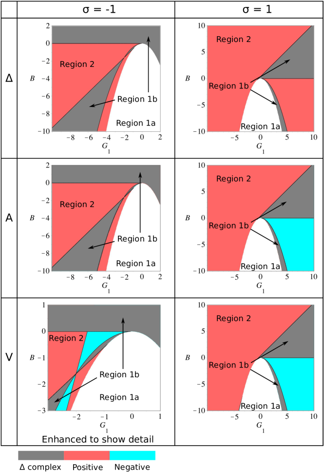
Figure 7: (color online) The parameter plane $(B,G_{1})$ for the cases $\sigma=\pm 1$ in equation (33) where soliton solutions in the form of (16) can exist in region 2. Region 1a and region 1b denote areas where $\Delta$ is complex. Subsequent panels show subregions of region 2, where soliton speed or amplitude is positive (red) or negative (blue). The images for $\Delta$ use red shading for region 2, for reference. We use an enhanced scale in the lower left frame for $V$ to show detail.

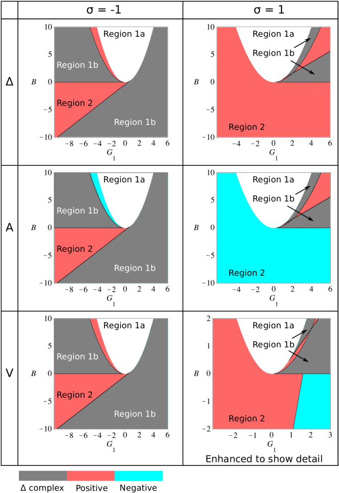
Figure 8: (color online) The parameter plane $(B,G_{1})$ for the cases $\sigma=\pm 1$ in equation (33) where soliton solutions in the form of (16) can exist in region 2. Region 1a and region 1b denote areas where $\Delta$ is complex. Subsequent panels show subregions of region 2, where soliton speed or amplitude is positive (red) or negative (blue). The images for $\Delta$ use red shading for region 2, for reference. We use an enhanced scale in the lower right frame for $V$ to show detail.

Thus, we see that nonlinear dispersion can affect the existence of soliton solutions, their nature (regular or embedded solitons), polarity, and, apparently, stability, as discussed in section IV.

IV Numerical solutions for stationary solitons

Soliton solutions derived in the previous section represent particular cases of the wide family of stationary solutions containing a class of solitary waves. Solitary wave solutions of equation (2) (or in the stationary case equation (13)) can be constructed, in general, by means of one of the well-known numerical methods, e.g., the Petviashvili method Petviashvili92 ; Pelinovsky04 or Yang–Lacoba method Yang08 . As mentioned in the Introduction, in some particular cases soliton solutions were found analytically, in other cases numerically. In the particular case of the Gardner–Kawahara equation, when $\gamma_{1}=\gamma_{2}=0$ in equation (2) (or $G_{1}=G_{2}=0$ in equation (13)), soliton solutions were constructed and studied in Kurkina15 .

Here we will construct a family of soliton solutions using the Petviashvili method for some particular cases to compare the numerical solutions with the analytical solutions derived in the previous section. The numerical method in application to equation (13) is described in Appendix B. We consider two particular cases when $G_{1}=G_{2}=0$ and when $G_{2}=3G_{1}$. In the latter case we will see the influence of nonlinear dispersion on the shape and polarity of solitary waves.

IV.1 The Gardner–Kawahara equation ($G_{1}=G_{2}=0$)

We showed in Section III.2 that embedded solitons of the form (16) can exist in the Gardner–Kawahara equation under certain restrictions on the value of $B$, and these restrictions are different for $s=-1$ and $s=1$. We therefore split the following analysis into two subsections.

IV.1.1 Numerical solutions in the case of negative cubic term ($s=-1$)

In this case soliton solutions in the form of equation (16) can exist only for $B>2/5$ and represent the embedded soliton. However, soliton solutions in different forms can exist both for positive and negative $B$. For positive $B$ such solutions can be constructed numerically for $V<V_{min}\equiv-1/(4B)$ (see Figure 2). In Figure 9 we present two families of numerical solutions. In panel (a) one can see the analytical solution for the embedded soliton (16) (line 1) when $B=8/5$ and the soliton has the minimum width $\Delta_{min}=\sqrt{32}$ and speed $V=3/20$ (see Subsection III.2). Lines 2, 3, and 4 show numerically constructed regular solitons for the same value of $B$ and $V=-0.25$, $-0.5$, and $-1$ respectively.

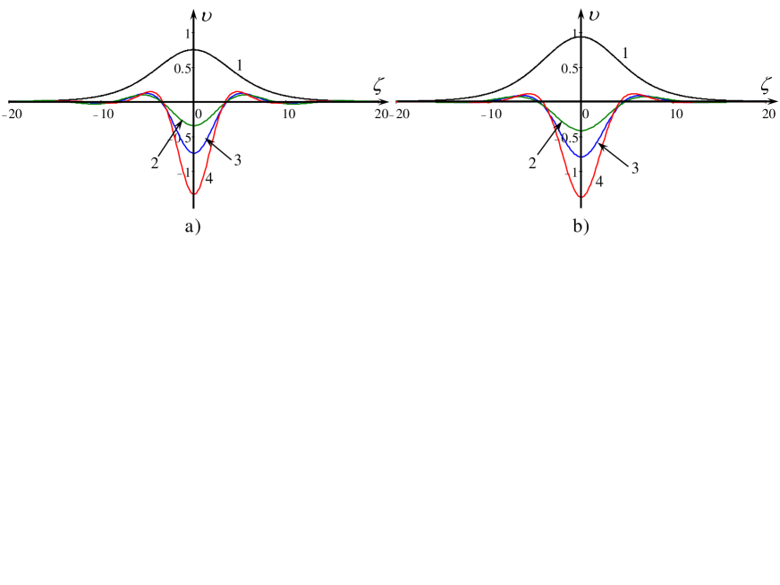
Figure 9: (color online) Soliton profiles in the case $G_{1}=G_{2}=0$. Panel (a) $B=8/5$: the embedded soliton (16) (line 1), other lines represent regular solitons for $V=-0.25$ (line 2), $V=-0.5$ (line 3), and $V=-1$ (line 4). Panel (b) $B=128/45$: the embedded soliton (16) (line 1), other lines represent regular solitons for $V=-0.25$ (line 2), $V=-0.5$ (line 3), and $V=-1$ (line 4).

In panel (b) one can see the analytical solution for the embedded soliton (16) (line 1) when $B=128/45$ and the soliton has the maximal speed $V=5/32$ and width $\Delta=16\sqrt{2/15}$ (see Subsection III.2). Lines 2, 3, and 4 show numerically constructed regular solitons for the same value of $B$ and $V=-0.25$, $-0.5$, and $-1$ respectively.

When $B<2/5$ analytical solutions of equation (13) are unknown, however they can be constructed numerically. We managed to construct such solutions within a relatively narrow range of parameters. In particular, when $B=1/5$, solitary-type solutions appear in the form of oscillatory wave trains – see Figure 10a (similar solutions were constructed numerically in Champneys97 ). When $V$ approaches $-1.25$ from below, solitons look like envelope solitons of the non-linear Schrödinger (NLS) equation (see, e.g. Whitham74 ; Karpman75 ; Lamb80 ; Ablowitz81 ; Dodd82 ; Newell85 ). Then, when $V$ decreases, the soliton shape smoothly changes and represents a negative polarity soliton with oscillatory tails as shown by line 2 in Figure 10a. We did not manage to construct numerical solutions for $V<-1.7$.

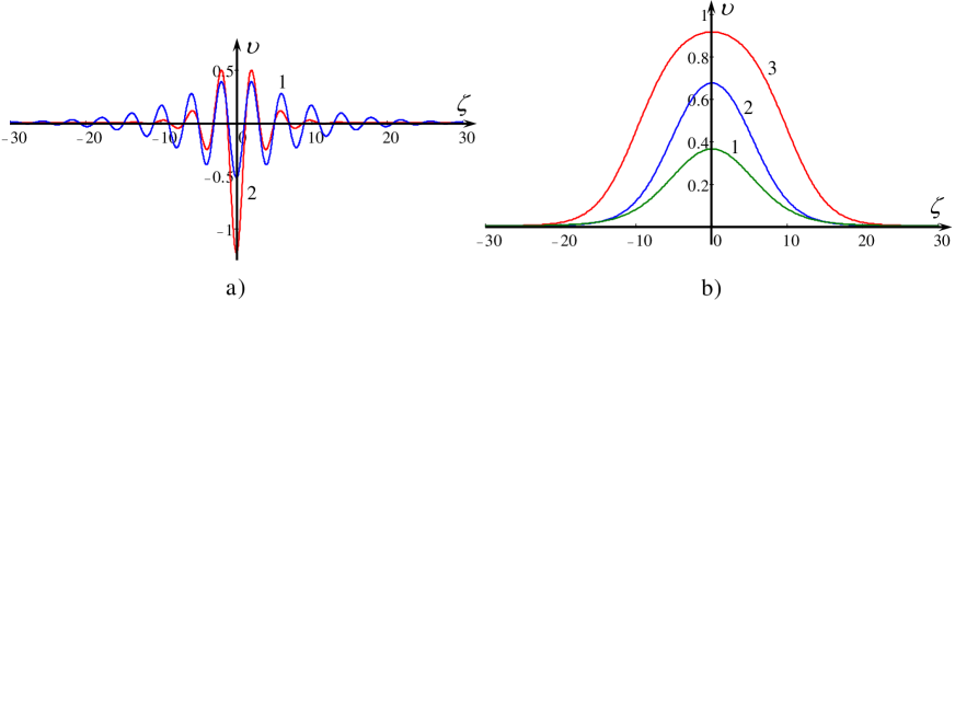
Figure 10: (color online) Soliton profiles in the case $G_{1}=G_{2}=0$. Panel (a) shows solitons for $B=1/5$ and speed $V=-1.3$ (line 1) or $V=-1.6$ (line 2). Panel (b) shows solitons for $B=-1$ and speed $V=0.1$ (line 1), $V=0.15$ (line 2) or $V=0.17$ (line 3).

When $B<0$ regular solitons exist for $V>0$ and have bell-shaped profiles as shown in Figure 10b for $B=-1$ and several values of $V$. However, they exist only within a relatively narrow range of $V$ between $0$ and $0.17$. Similar situation occurs for other negative values of $B$.

IV.1.2 Numerical solutions in the case of positive cubic term ($s=1$)

In this case solutions in the form of (16) can exist only for negative $B$; they can be in the form of either regular solitons or embedded solitons (see Subsection III.2). However soliton solutions in different forms can exist, in principal, both for positive and negative $B$. Nevertheless we did not manage to construct soliton solutions numerically for positive $B$. This requires further investigation.

In the case of negative $B$ there are two families of regular solitons of positive and negative polarities. Typical examples are shown in Figure 11 for $B=-0.1$. Line 1 represents the analytical solution (16) with $V=2.1$ and line 2 is another analytical solution with $V=0.9$ as per equation (28). However, we failed to reproduce these solutions numerically by means of the Petviashvili method. Lines 3 and 5 in Figure 11 correspond to solutions found using the numerical scheme for $V=2.1$ and $V=0.9$ respectively (in comparison to the analytical solutions of line 1 and line 2). All these solitons have exponentially decaying asymptotics at infinity.

To explain the difference in the solutions, we refer to equation (14). As follows from the analysis of this equation, all its roots are real when $0<V<-1/(4B)$ (which is the case for Figure 11). This means that exponential decay of a solitary wave can be controlled by one of two real roots at plus infinity and one of the other two roots at minus infinity. Apparently, soliton solutions obtained analytically and numerically correspond to different roots of characteristic equation (14).

Then, it follows from numerical solutions that when the soliton speed increases, so does the amplitude, but the soliton profile becomes non-monotonic; this is again in agreement with the qualitative analysis shown in Figure 3a for $B<0$. Lines 4 and 6 illustrate such solutions for $V=100$.

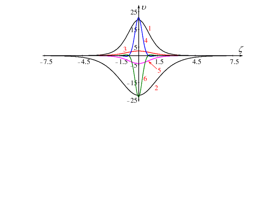
Figure 11: (color online) Soliton profiles in the case of positive cubic nonlinearity, $s=1$, with $G_{1}=G_{2}=0$ and $B=-0.1$. Lines 1 and 2 show analytical solutions (16) for regular solitons with $V=2.1$ for the positive polarity soliton and $V=0.9$ for the negative polarity soliton. Lines 3 and 5 pertain to the numerical solutions with $V=2.1$ and $V=0.9$ correspondingly, and lines 4 and 6 pertain to solutions with $V=100$.

We did not manage to construct solitons of negative polarity with $B=-0.1$ and $V<1.95$ even when the starting solution for the iteration scheme (see Appendix B) was chosen in the form of the analytical solution (16). However, for $V\geq 1.95$, solitons of negative polarity were constructed numerically and are shown in Figure 11. They represent almost mirror reflections of solitons of positive polarity. A similar situation occurs in the case of the Gardner equation with positive cubic nonlinearity, when solitons of positive polarity can exist for all amplitudes from 0 to infinity, whereas solitons of negative polarity cannot exist, if their amplitudes are less then some critical value. Below the critical amplitude breathers can exist instead (see, e.g., OstrEtAl15 and references therein).

IV.2 The particular case of equation (13) with $G_{2}=3G_{1}$

Another particular case we study is $G_{2}=3G_{1}$. The basic equation (13) in this case contains four independent parameters $B$, $G_{1}$, $s$, and $V$, which determine the structure of solitary waves. This case is convenient from the numerical point of view as the iteration scheme is simpler than for other cases of $G_{1}$ and $G_{2}$. Another point of interest in this case is the fact that wave energy is not conserved in general – see equation (11) (whereas for even solutions the energy is conserved), therefore this allows us to understand the role of nonlinear dispersion. In the parameter plane $(G_{1},B)$ there are zones where regular solitons of different polarity can exist. The boundaries of these zones are fairly complicated and we demonstrate some typical soliton solutions belonging to different zones, for the cases when $s=-1$ and $s=1$ as before.

IV.2.1 Numerical solutions in the case of negative cubic term ($s=-1$)

• $B=-1$

Consider first the case when $B=-1$ in equation (13). In this case regular solitons can exist for $V>0$. In Figure 12 we illustrate the structure of a solitary wave when $G_{1}$ varies. Line 1 in both panels show the reference case when $G_{1}=0$. If this parameter becomes negative, the solitons become wider, their amplitudes slightly decrease, and the tops become flatter (see lines 2 and 3 in panel a). However, when $G_{1}$ approaches $-9$, the soliton profiles become non-monotonic with oscillations on the top (see line 4 in panel a) (similar solutions were constructed numerically in Champneys97 ). For smaller values of $G_{1}<-9$ we were unable to obtain numerical solutions (apparently, they do not exist for such a set of parameters).

When $G_{1}$ becomes positive and increases the solitons become narrower, their amplitudes slightly increase first, but then they monotonically decrease when $G_{1}$ exceeds 4 (see lines 1, 2, and 3 in panel b). For relatively large values of $G_{1}$ soliton tails become non-monotonic with negative minima on the profile (see line 4 in panel b).

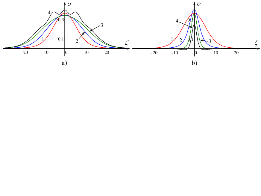
Figure 12: (color online) Numerical solutions of equation (13) for negative cubic nonlinearity ($s=-1$), $B=-1$, $V=0.1$, $G_{2}=3G_{1}$, and several values of $G_{1}$. In panel (a) we have the soliton solution for $G_{1}=0$ (line 1, reference case), $G_{1}=-4$ (line 2), $G_{1}=-8$ (line 3) and $G_{1}=-9$ (line 4). In panel (b) we have the soliton solution for $G_{1}=0$ (line 1, reference case), $G_{1}=4$ (line 2), $G_{1}=8$ (line 3) and $G_{1}=16$ (line 4).

• $B=1$

When $B=1$ solutions in the form of regular solitons can exist only for negative $V<V_{min}\equiv-1/(4B)$ (see after equation (12)). In Figure 13a we show the structure of solitary waves for $V=-0.5$ and different values of $G_{1}$. Solitons in this case have negative polarity and oscillating tails. Line 1 corresponds to the case when $G_{1}=0$. If this parameter becomes negative, the solitons become wider and their amplitudes increase (see line 2 in panel a). For $G_{1}<-3$ we were unable to construct numerical solutions (apparently, they do not exist for such a set of parameters). When $G_{1}$ becomes positive and increases, the solitons become narrower and smaller (see lines 3 and 4 in panel a).

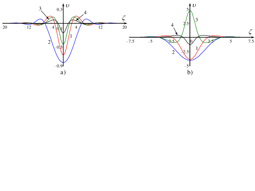
Figure 13: (color online) Numerical solutions of equation (13) for negative cubic nonlinearity ($s=-1$), $B=1$, $G_{2}=3G_{1}$, and several values of $G_{1}$. Panel (a): $V=-0.5$ and we have the soliton solution for $G_{1}=0$ (line 1, reference case), $G_{1}=-3$ (line 2), $G_{1}=3$ (line 3) and $G_{1}=12$ (line 4). Panel (b): $V=-5$ and we have the soliton solution for $G_{1}=0$ (line 1, reference case), $G_{1}=-1.88$ (line 2), $G_{1}=-1.89$ (line 3) and $G_{1}=12$ (line 4).

In Figure 13b we show the structure of solitary waves for $V=-5$ and different values of $G_{1}$. Solitons in this case can have both negative and positive polarity; they can have slightly oscillating tails or non-monotonic aperiodic tails. Line 1 corresponds to the case when $G_{1}=0$. If this parameter becomes negative and varies from zero to $G_{1}=-1.88$, the solitons remain qualitatively the same, but become wider and their amplitudes slightly increase as shown in panel b) by line 2. When $G_{1}$ further decreases and becomes less than $-1.89$, the solitons abruptly change their polarity, become taller and narrower with well-pronounced negative minima (see line 3). Further increases in $G_{1}$ result in soliton profiles that remain qualitatively the same, but their amplitudes decrease.

When $G_{1}$ becomes positive and increases, soliton profiles remain similar to the shape of the soliton for $G_{1}=0$, but the solitons become narrower and of smaller amplitude (see, e.g., line 4 in panel b).

IV.2.2 Numerical solutions in the case of positive cubic term ($s=1$)

In this case the analytical solution (16) for $B>0$ can exist only for $V>0$ representing an embedded soliton (see Figure 2 and Figure 8), whereas solutions in the form of regular solitons, apparently, cannot exist; we were unable to construct such solutions numerically.

For $B<0$ the analytical solution (16) exists in the form of a regular soliton for $V>0$ and embedded soliton for $V<0$ (see Figure 2 and Figure 8). Embedded solitons cannot be reproduced by means of the Petviashvili method (see Appendix B), therefore we constructed only regular solitons numerically for the particular case of $B=-1$ and $V>0$. The structure of these solitons depends on their speed and is illustrated by Figure 14 for two particular values of $V$. In panel (a) we show a few typical soliton profiles for $V=0.1$ and several values of $G_{1}$. Line 1 shows the reference case when $G_{1}=0$. If $G_{1}$ becomes negative, the solitons become wider and their amplitudes slightly decrease (see line 2). For $G_{1}<-12$ we did not obtain soliton solutions.

When $G_{1}$ becomes positive, the soliton amplitude slightly increases first (see line 3), but then it decreases, and solitons become narrower (see line 4). For sufficiently large $G_{1}$ solitons profiles become non-monotonic, so that negative minima appear in the profiles (see line 5).

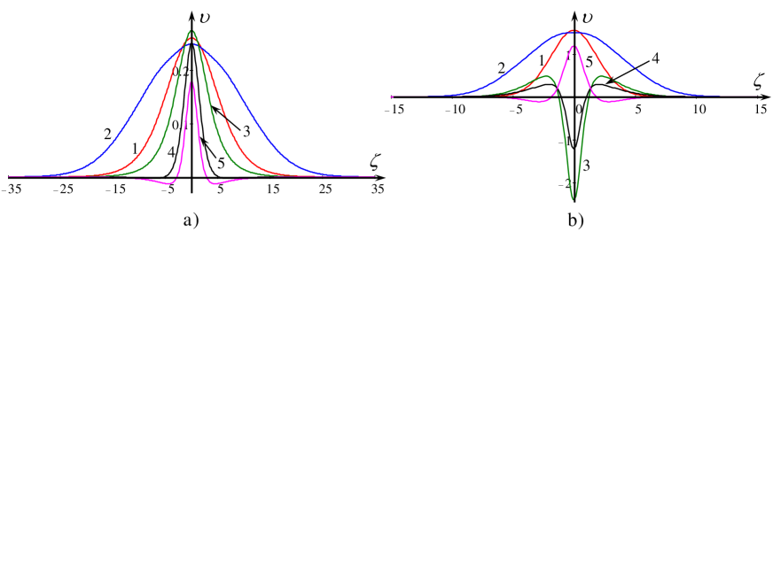
Figure 14: (color online) Numerical solutions of equation (13) for positive cubic nonlinearity ($s=1$) and $G_{2}=3G_{1}$, $B=-1$. Panel (a): $V=0.1$ and we have the soliton solution for $G_{1}=0$ (line 1, reference case), $G_{1}=-12$ (line 2), $G_{1}=4$ (line 3), $G_{1}=12$ (line 4) and $G_{1}=24$ (line 5). Panel (b): $V=1$ and we have the soliton solution for $G_{1}=0$ (line 1, reference case), $G_{1}=-4.63$ (line 2), $G_{1}=-4.64$ (line 3), $G_{1}=-12$ (line 4) and $G_{1}=6$ (line 5).

In panel (b) we show other typical soliton profiles for $V=1$ and several values of $G_{1}$. Line 1 shows the reference case when $G_{1}=0$. If $G_{1}$ becomes negative, the solitons become wider and their amplitudes slightly decrease (see line 2). When $G_{1}$ passes through some critical value between $-4.63$ and $-4.64$ the soliton polarity abruptly alters from positive to negative (see line 3). Then, when $G_{1}$ further decreases, soliton profiles remain qualitatively similar to what is shown by line 3, but their amplitudes become smaller (see line 4). When $G_{1}$ becomes positive soliton profiles remain qualitatively similar to line 1, but their amplitudes gradually decrease and well-pronounced minima appear on both sides of the crests (see line 5).

The solutions constructed numerically do not reproduce the analytical solution (16). The reason is the same as discussed in Section IV.1.2 i.e. solutions with different asymptotics can coexist for the same set of parameters, and the numerical scheme, apparently, converges to only one of them which is different from solution (16).

IV.3 Stationary solutions for two particular cases of equation (9)

In this subsection we briefly consider particular exact solutions of equation (9). In the first case we set $s=G_{1}=G_{2}=0$ to reduce the general equation (9) to the generalised Kawahara equation containing both third- and fifth-order derivatives. The exact solution to this equation was obtained for the first time by Yamamoto & Takizawa Yamamoto81 (for further references see also Kichenassamy92 )

$$\upsilon\left(\zeta\right)=-\frac{105}{169B}\mathop{\rm sech}\nolimits^{4}\left(\frac{x-V\tau}{\Delta}\right),$$ (34)

where $V=-36/169B$, $\Delta=\sqrt{-52B}$ and $B<0$. There are no free parameters in this solution; the amplitude, speed and width of Yamamoto–Takizawa (YT) soliton (34) are determined by the coefficients of the generalised Kawahara equation. The soliton moves with a positive speed, whereas linear waves propagate with negative phase speeds, therefore it is a regular soliton; its profile is shown in Figure 15 by line 1 for $B=-1$. It was easily reproduced numerically with the help of the Petviashvili method when the speed was chosen in accordance with the formula $V=-36/169$, $B\approx 0.213$.

By means of Petviashvili’s method we constructed a family of soliton solutions with the fixed value of parameter $B=-1$. All solitary solutions of this family are qualitatively similar to the YT soliton. In particular, line 2 shows the numerical solution for $V=0.25$, and line 3 for $V=0.15$. It was discovered that the soliton amplitude decreases as the speed decreases. At small amplitudes the soliton profile becomes indistinguishable from the profile of the KdV sech²-soliton of the same amplitude. This is illustrated by Figure 15 where the numerically obtained line 3 practically coincides with line 4, which represents the KdV soliton of the same amplitude. Apparently within this equation there is a continuous family of solitary wave solutions whose profiles depend on their amplitude, and the YT soliton is just one particular of the representatives of this family.

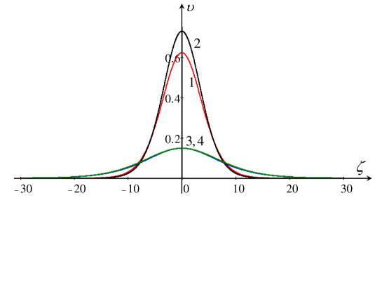
Figure 15: (color online) Yamamoto–Takizawa soliton (34) (line 1). Other lines represent numerically obtained soliton solutions of equation (9) with $s=G_{1}=G_{2}=0$ and $B=-1$. The solution with $V=0.25$ and $V=0.15$ correspond to line 2 and line 3 respectively, and line 4 represents the KdV soliton with the same amplitude as line 3.

Because the generalised Kawahara equation is non-integrable, one can expect that soliton interactions are inelastic, i.e. in the process of soliton collisions they radiate small-amplitude trailing waves and, as a result, change their parameters. This will be confirmed in Section V.

In the second case we present the soliton solution to the Kaup–Kupershmidt equation Dodd82 ; Newell85 ; Kichenassamy92 . This equation is a particular case of equation (2) with the following coefficients: $\alpha=\beta=0$, $\varepsilon\alpha_{1}=180$, $\varepsilon\gamma_{1}=30$, $\varepsilon\gamma_{2}=75$, and $\varepsilon\beta_{1}=1$. With such a set of coefficients the equation is completely integrable, and its soliton solution has a slightly unusual form:

$$\upsilon(\xi,\tau)=3A\frac{4\mathop{\rm sech}\nolimits^{2}\left(\zeta/\Delta\right)-\mathop{\rm sech}\nolimits^{4}\left(\zeta/\Delta\right)}{\left[2+\mathop{\rm sech}\nolimits^{2}\left(\zeta/\Delta\right)\right]^{2}},$$ (35)

where $A$ is the soliton amplitude (a free parameter), $\Delta=1/\sqrt{6A}$ is the soliton width, $\zeta=\xi-V\tau$, and $V=(6A)^{2}$ is the soliton speed.

The profile of the Kaup–Kupershmidt (KK) soliton of a unit amplitude is shown in Figure 16. As one can see, its speed is positive, whereas waves of infinitesimal amplitude within the Kaup–Kupershmidt equation have negative phase speeds (in the moving coordinate frame). Therefore, the KK soliton is a regular soliton too.

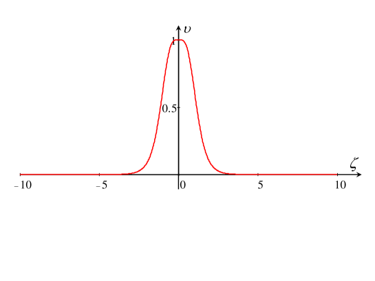
Figure 16: (color online) The Kaup–Kupershmidt “fat” soliton (35) of a unit amplitude.

In contrast to the previous case, the Kaup–Kupershmidt equation is completely integrable, therefore soliton interactions are elastic, and to a certain extant, trivial. This means that after interaction solitons completely restore their original parameters and do not radiate small amplitude perturbations. Therefore, solitons remain the same as they were before interaction, and the only traces of interaction are their shifts in space and time, exactly as in the interaction of elastic particles.

V Numerical study of soliton interactions

It was anticipated in Kichenassamy92 that equation (2) would be studied numerically to confirm existence and robustness of solitary wave solutions, investigate whether they emerge evolutionary from the arbitrary initial pulse-type perturbations, how do they behave under collisions, whether “they emerge unscathed as true solitons, or is there a small, but nonzero nonelastic effect”. Since that time such investigation was not carried out to the best of our knowledge. Here we will try to illuminate these issues.

To solve equation (2) numerically, we apply a pseudospectral technique similar to that used in Grimshaw08 ; Alias13 ; Alias14 ; Khusnutdinova17 . The equation is solved in the Fourier space using a 4 order Runge–Kutta method for time stepping, while the nonlinear terms are calculated in the real space and transformed back to the Fourier space for use in the Runge–Kutta scheme. To remove the aliasing effects, we use the truncation 2/3-rule by Orszag in Boyd Boyd01 . See Appendix C for the description of the numerical scheme.

To generate solitons for a given set of parameters, an initial pulse was taken as the initial condition. This pulse was taken in the form a standard KdV soliton i.e. of the form

$$u(x,0)=P\mathop{\rm sech}\nolimits^{2}\left(\sqrt{\frac{\lvert P\rvert}{12}}\frac{x}{L}\right),$$ (36)

where $P$ corresponds to the amplitude and $L$ is a factor used to change the width of this initial pulse. In each case, we can control the number of solitons produced, and their amplitudes, via the parameters $P$ and $L$.

To calculate the interaction of regular or embedded solitons, we generate regular solitons of the required amplitude using the method described above. Once the solitons generated from the pulse are well separated, we extract them from the solution. To study the interaction of these regular solitons with other regular solitons or embedded solitons, we generate an initial condition using the extracted soliton and either another extracted soliton (for the interaction of regular solitons) or with the embedded soliton found analytically, so that their interactions could be studied. This extraction was performed so that any radiation emerging from the initial pulse would not interfere with the collision. In each of the numerical cases considered below, the value of $P$ and $L$ are stated for each regular soliton generated via this method. Furthermore, we state if the solitons used in the proceeding calculations are found analytically or generated from a pulse.

With the help of this numerical method we studied interactions of solitary waves with different parameters and different coefficients of the governing equation (9). First of all we found that the embedded soliton propagates in all cases, with minimal loss of energy. We have calculated the change of “wave energy” $I_{2}=\int(u^{2}/2)\;\mathrm{d}x$ (see Introduction) as

$$\Delta I_{2}=\frac{I_{2}(t)-I_{2}(0)}{I_{2}(0)},$$ (37)

where $I_{2}(0)$ is the initial wave energy and $I_{2}(t)$ is the wave energy at time $t$.

Using this numerical method with periodic boundary conditions, we obtained $\Delta I_{2}=1.2\cdot 10^{-13}$ and $2.4\cdot 10^{-13}$ for the embedded solitons in the cases when nonlinear dispersion is present, whereas for the regular solitons in these cases we obtained $\Delta I_{2}=1.2\cdot 10^{-5}$ and $5.2\cdot 10^{-6}$. In the case of the regular solitons, as they were generated by a pulse-like initial condition, fast moving radiation was generated that would re-enter the domain and interfere with the main wave structure. To diminish this effect, we applied “a sponge layer” to the solution domain to absorb this radiation and prevent it re-entering the solution domain, as detailed in Appendix C. This accounts for the lower accuracy in the wave energy conservation. It is worth noting that when the embedded soliton is perturbed, the energy is no longer conserved and therefore the solution eventually breaks down, except in the case when there is no nonlinear dispersion (see Section V.1 below).

For the regular solitons in all cases, they steadily propagate without loss of energy even in the cases when $G_{2}\neq 2G_{1}$. As has been mentioned above (see the paragraph after equation (11)), in the case of propagation of a stationary wave described by an even function, the right-hand side of equation (11) vanishes, and wave energy $I_{2}$ is conserved. However, an interesting question arises about the energy conservation in the process of soliton interaction when $G_{2}\neq 2G_{1}$. Below we present the results of our numerical study of equation (9) with negative cubic nonlinearity in the cases when (i) $G_{1}=G_{2}=0$ and (ii) $G_{2}=3G_{1}$. Equation (9) with positive cubic nonlinearity can be studied in a similar way, but such exercises require much more computational resources, because soliton amplitudes are limited in this case and can be very close to each other, whereas their speeds are relatively small, therefore soliton interactions take a very long time to compute.

V.1 The Gardner–Kawahara equation ($G_{1}=G_{2}=0$)

As shown in subsection IV.1.1, there are families of regular solitons for positive and negative $B$, some of which can co-exist with the embedded soliton (16) – see Figures 9 and 10. Here we present (i) an example of pulse disintegration into a number of regular solitons (Figure 17); (ii) interaction of regular solitons (Figure 18); and (iii) interaction of regular and embedded solitons (Figure 19). Figure 17 illustrates that regular solitons with non-monotonic profiles asymptotically appear from pulse-type initial perturbations in the process of its disintegration. Apparently, such solitons can form bound states, the bi-solitons, triple-solitons, or multi-solitons, i.e., stationary moving formations consisting of two or more binding solitons Gorshkov76 ; Gorshkov79 ; Champneys97 ; Obregon98 ; Kurkina15 , but we did not study this phenomenon in our paper.

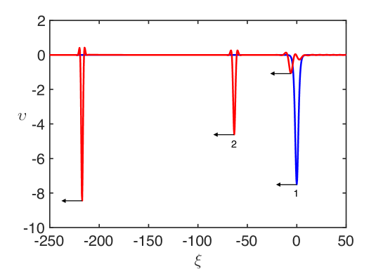
Figure 17: (color online) Generation of several regular solitons from the initial sech²-pulse within the framework of equation (9) with $s=-1$, $B=8/5$, $G_{1}=G_{2}=0$. Line 1 corresponds to the initial condition at $t=0$ (blue) and line 2 is the solution at $t=10$ (red). The initial pulse parameters are $P=-7.5$ and $L=1$.

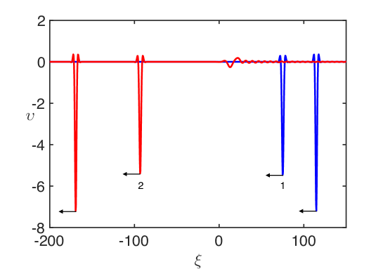
Figure 18: (color online) Interaction of two regular solitons within the framework of equation (9) with $s=-1$, $B=8/5$, $G_{1}=G_{2}=0$. Line 1 corresponds to the initial condition at $t=0$ (blue) before the interaction and line 2 to the solution after the interaction at $t=20$ (red). Both solitons were obtained numerically from a pulse-like initial condition. The initial pulse parameters are $P_{1}=-7.5$ and $L_{1}=1$ for the taller soliton and $P_{2}=3P_{1}/4$ and $L_{2}=1$ for the shorter soliton.

The interaction of two solitons as shown in Figure 18 demonstrates that the solitons survive after the collision, but a residual small wave packet is generated in the trailing wave field. This clearly indicates that the soliton collision is inelastic.

The most fascinating is Figure 19 which demonstrates (seemingly for the first time) that the embedded soliton can survive after interaction with a regular soliton. The interaction is obviously inelastic, so that small disturbances appear both in front and behind the embedded soliton. Thus, we see that it survives even after collision with a regular soliton, and for much longer times (up to $t=700$) the embedded soliton keeps its identity.

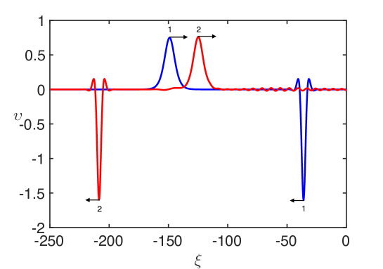
Figure 19: (color online) Interaction of a regular soliton of negative polarity and an embedded soliton of positive polarity within the framework of equation (9) with $s=-1$, $B=-8/5$, $G_{1}=G_{2}=0$. Line 1 corresponds to the initial condition at $t=0$ (blue) before the interaction and line 2 to the solution after the interaction at $t=140$ (red). The regular soliton was obtained numerically from a pulse-like initial condition. The initial pulse parameters are $P=-7.5$ and $L=1$.

V.2 Interactions of solitary waves when $G_{2}=3G_{1}$

Following the same steps as in subsection V.1, we consider the cases when the parameters are (i) $s=-1$, $B=-1$, $G_{1}=4$, and $G_{2}=12$ (see Figure 12b) and (ii) $s=-1$, $B=1$, $G_{1}=-1.88$, and $G_{2}=-5.64$ (see Figure 13b). First of all we observed steady propagation of solitons in both of these cases. Then we observed the emergence of a number of solitons from an initial pulse with larger amplitude and width; this is illustrated in Figure 20 for case (i) and Figure 21 for case (ii).

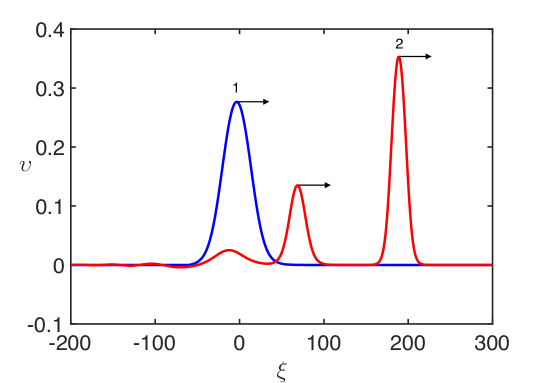
Figure 20: (color online) Generation of regular solitons from the initial sech²-pulse within the framework of equation (9) with $s=-1$, $B=-1$, $G_{1}=4$ and $G_{2}=12$. Line 1 corresponds to the initial condition at $t=0$ (blue) and line 2 is the solution at $t=1800$ (red). The initial pulse parameters are $P=0.275$ and $L=3.175$.

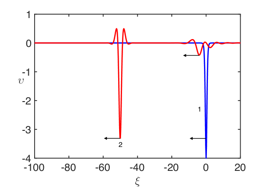
Figure 21: (color online) Generation of regular solitons from the initial sech²-pulse within the framework of equation (9) with $s=-1$, $B=1$, $G_{1}=-1.88$ and $G_{2}=-5.64$. Line 1 corresponds to the initial condition at $t=0$ (blue) and line 2 is the solution at $t=10$ (red). The initial pulse parameters are $P=-4$ and $L=0.3$.

Finally we studied the interaction of these solitons. When colliding two regular solitons, we observed that after the interaction both the solitons survive, but some portion of their energy converts into a small wave packet generated in the trailing wave field; this is shown in Figure 22 for case (i) and Figure 23 for case (ii). This is typical for the inelastic interaction.

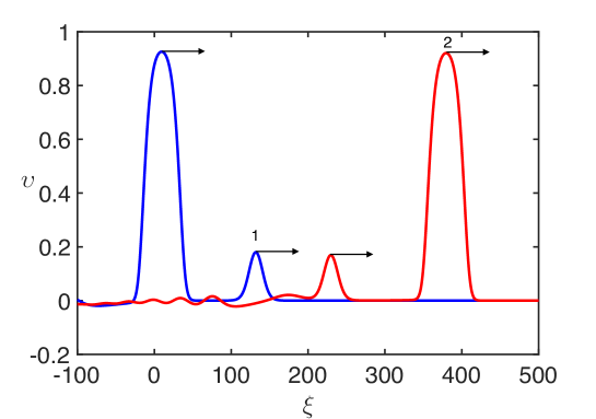
Figure 22: (color online) Interaction of two regular solitons within the framework of equation (9) with $s=-1$, $B=-1$, $G_{1}=4$ and $G_{2}=12$. Line 1 corresponds to the initial condition at $t=0$ (blue) before the interaction and line 2 to the solution after the interaction at $t=2100$ (red). Both solitons were obtained numerically from a pulse-like initial condition. The initial pulse parameters are $P_{1}=1.2$ and $L_{1}=5$ for the taller soliton and $P_{2}=P_{1}/3$ and $L_{2}=1$ for the shorter soliton.

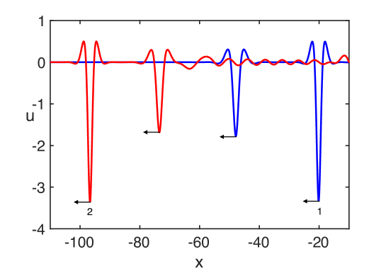
Figure 23: (color online) Interaction of two regular solitons within the framework of equation (9) with $s=-1$, $B=1$, $G_{1}=-1.88$ and $G_{2}=-5.64$. Line 1 corresponds to the initial condition at $t=0$ (blue) before the interaction and line 2 to the solution after the interaction at $t=15$ (red). Both solitons were obtained numerically from a pulse-like initial condition. The initial pulse parameters are $P_{1}=-4$ and $L_{1}=0.3$ for the taller soliton and $P_{2}=P_{1}/2$ and $L_{2}=0.3$ for the shorter soliton.

For the collision of a regular soliton with an embedded soliton, in case (i) we observed that only the regular soliton survives the collision and an intense wave packet is generated in the trailing wave field (see Figure 24).

In contrast to that, in case (ii), the regular and embedded solitons both survive after the collision and a wave packet is generated in front of the embedded soliton (see Figure 25). In both cases we conclude that the collision is inelastic. It is worth noting in this case that our numerics were not stable beyond the time considered in the calculation; it may be stable for a smaller spatial discretisation, however the corresponding time discretisation becomes very small and the calculations take a very long time.

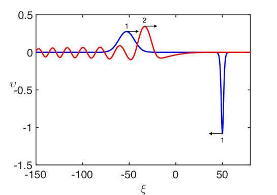
Figure 24: (color online) Interaction of regular soliton of positive polarity and embedded soliton of negative polarity within the framework of equation (9) with $s=-1$, $B=-1$, $G_{1}=4$ and $G_{2}=12$. Line 1 corresponds to the initial condition at $t=0$ (blue) before the interaction and line 2 to the solution after the interaction at $t=250$ (red). The regular soliton was obtained numerically from a pulse-like initial condition. The initial pulse parameters are $P=0.4$ and $L=1$. The gap soliton survives, but the embedded soliton does not.

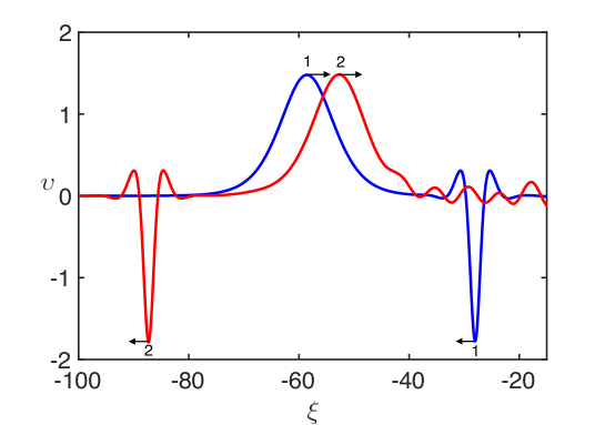
Figure 25: (color online) Interaction of regular soliton of negative polarity and embedded soliton of positive polarity within the framework of equation (9) with $s=-1$, $B=1$, $G_{1}=-1.88$ and $G_{2}=-5.64$. Line 1 corresponds to the initial condition at $t=0$ (blue) before the interaction and line 2 to the solution after the interaction at $t=30$ (red). The regular soliton was obtained numerically from a pulse-like initial condition. The initial pulse parameters are $P=0.4$ and $L=1$.

V.3 The generalised Kawahara equation

As we defined in Section IV.3 above, the generalised Kawahara equation is a particular case of equation (9) with the coefficients $s=G_{1}=G_{2}=0$. We analysed the stationary solitary solutions, one of which is the YT soliton (34). Here we show that solitary waves emerge from pulse-type initial perturbations within the generalised Kawahara equation. As the initial condition the sech² pulse was chosen. Figure 26 illustrates an example of pulse disintegration onto two solitary waves accompanied by small residual wave train (not visible in the figure).

The soliton interaction is demonstrated in Figure 27. The initial condition was chosen as the YT soliton (1) and the numerically obtained solitary wave (2). We see that solitary waves survive the collision and appear after that with almost the same amplitudes. However, a small wave train appears in the result of interaction, evidence that the interaction is inelastic.

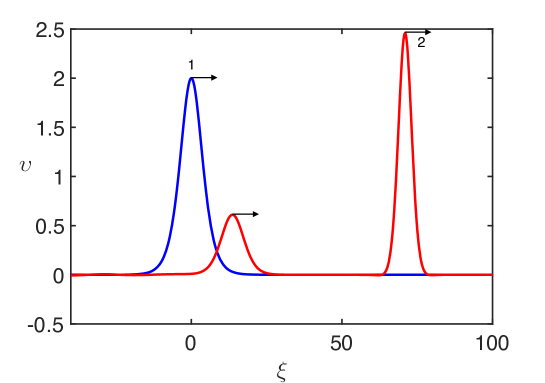
Figure 26: (color online) Generation of solitons from the initial sech²-pulse for the generalised Kawahara equation. Line 1 corresponds to the initial condition at $t=0$ (blue) and line 2 is the solution at $t=80$ (red). The initial pulse parameters are $P=2$ and $L=2$.

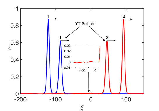
Figure 27: (color online) Interaction of the YT regular soliton (smaller amplitude pulse in the figure) with another regular solitary wave numerically constructed within the framework of generalised Kawahara equation. Line 1 corresponds to the initial condition at $t=0$ (blue) before the interaction and line 2 to the solution after the interaction at $t=680$ (red). The regular soliton with the framework of the generalised Kawahara equation was obtained numerically from a pulse-like initial condition. The initial pulse parameters are $P=1$ and $L=1$. Small insertion shows a magnified fragment of a radiated wave field.

VI Conclusion

In this paper we have studied the properties of soliton solutions of the fifth-order KdV equation (2) which is used to describe surface and internal gravity waves, as well as appearing in other applied areas. Using the changes of independent and dependent variables this equation has been reduced to the dimensionless form (9) with the minimum number of independent parameters, only three for positive and negative cubic nonlinearity. In the theory of nonlinear internal waves both these cases of positive and negative cubic nonlinearity can occur depending on the stratification of the fluid Talipova99 ; Apel07 ; RuvKurk14 . In some particular cases equation (9) reduces to well known equations, among which there are Gardner OstrEtAl15 , Kawahara Kawahara72 equations and their generalisation Giniyatullin14 ; Kurkina15 , Sawada–Kotera and Kaup–Kupershmidt equations Dodd82 ; Newell85 ; Kichenassamy92 .

Equation (9) is non-integrable, in general, and it does not provide conservation of the “wave energy”. However, it permits the existence of solitary wave solutions both with monotonic and non-monotonic profiles and even with oscillatory asymptotics, which suggests the existence of more complicated structures in the form of stationary multi-solitons Gorshkov76 ; Gorshkov79 ; Kurkina15 . Following Karczewska14 , we have derived an exact soliton solution in the general case and have shown that in some cases this solution can represent a regular soliton, whereas in others it represents an embedded soliton whose speed coincides with the speed of some linear wave. Our numerical simulations have confirmed that such solitons can propagate without loss of energy, if there are no perturbations in the form of other waves or medium inhomogeneity, or dissipation. We have identified the areas on the plane of parameters where the derived soliton solution exists as the embedded or regular soliton and found numerically a number of soliton solutions of equation (9) with different sets of governing parameters.

In the last section we have studied numerically the emergence of solitons from arbitrary pulse-type initial conditions and have demonstrated that regular solitons are generated from the initial conditions. However in the course of interaction such solitons produce small-amplitude trailing waves which evidences that the interaction has inelastic character. Moreover, the solitons with non-monotonic profiles can form stationary or non-stationary bound states similar to those experimentally observed in Gorshkov76 .

One particularly interesting observation emerging from our study is the stability of embedded solitons with respect to interactions with other waves (e.g., the regular solitons, like in this paper). This sheds some additional light on the stability problem and nature of embedded solitons and indicates that they could be observed in natural and laboratory environments. In particular, in the absence of nonlinear dispersion, the embedded soliton survives the interaction with no visible loss of amplitude. On the other hand, the results of our numerical investigations suggest that in some cases embedded solitons, apparently, can transfer to radiating solitons under the influence of external perturbations (the radiating solitons are quasi-stationary long-living solitary waves permanently radiating from one side small-amplitude linear waves – see, e.g., Grimshaw17 ; Khusnutdinova17 and references therein). We do not touch this interesting possibility in the present paper, but it can be a theme for further study.

Finally, it would be interesting to extend the present study to the study of the respective ring wave counterparts (see J ; L ; KZ_JFM ; KZ_PhysD and references therein). The solitary wave solutions studied in our present paper provide meaningful “initial conditions” for numerical experimentation with the amplitude equation describing ring waves.

Appendix A Coefficients of the Higher-Order KdV Equation for Water Waves

The coefficients of equation (2) for gravity surface waves are given in (3). Here we present the coefficients for internal waves in two-layer fluid derived in Giniyatullin14 . All notations are shown in Figure 1.

$$c =\sqrt{\frac{(\rho_{2}-\rho_{1})gh_{1}h_{2}}{\rho_{1}h_{2}+\rho_{2}h_{1}}},\quad\alpha=\frac{3c}{2h_{1}h_{2}}\frac{\rho_{2}h_{1}^{2}-\rho_{1}h^{2}_{2}}{\rho_{1}h_{2}+\rho_{2}h_{1}},\quad\beta=\frac{h_{1}h_{2}}{6}c\frac{\rho_{1}h_{1}+\rho_{2}h_{2}-3\sigma/c^{2}}{\rho_{1}h_{2}+\rho_{2}h_{1}},$$ (38)

$$\alpha_{1} =-\frac{3c}{8h_{1}^{2}h_{2}^{2}}\frac{\rho_{2}^{2}h_{1}^{4}+\rho_{1}^{2}h_{2}^{4}+2\rho_{1}\rho_{2}h_{1}h_{2}\left(4h_{1}^{2}+7h_{1}h_{2}+4h_{2}^{2}\right)}{\left(\rho_{1}h_{2}+\rho_{2}h_{1}\right)^{2}},$$ (39)

$$\beta_{1} =\frac{ch_{1}h_{2}}{90}\frac{\rho_{1}\rho_{2}\left(h_{1}^{4}+h_{2}^{4}+15h_{1}^{2}h_{2}^{2}/2\right)+\left(19/4\right)h_{1}h_{2}\left(\rho_{1}^{2}h_{1}^{2}+\rho_{2}^{2}h_{2}^{2}\right)-S_{1}}{\left(\rho_{1}h_{2}+\rho_{2}h_{1}\right)^{2}},$$ (40)

$$\gamma_{1} =\frac{c}{12}\frac{5h_{1}h_{2}\left(\rho_{2}^{2}h_{1}-\rho_{1}^{2}h_{2}\right)+\rho_{1}\rho_{2}\left(h_{1}-h_{2}\right)\left(7h_{1}^{2}+9h_{1}h_{2}+7h_{2}^{2}\right)-2S_{2}}{\left(\rho_{1}h_{2}+\rho_{2}h_{1}\right)^{2}},$$ (41)

$$\gamma_{2} =\frac{c}{24}\frac{23h_{1}h_{2}\left(\rho_{2}^{2}h_{1}-\rho_{1}^{2}h_{2}\right)+\rho_{1}\rho_{2}\left(h_{1}-h_{2}\right)\left(31h_{1}^{2}+39h_{1}h_{2}+31h_{2}^{2}\right)+2S_{2}/5}{\left(\rho_{1}h_{2}+\rho_{2}h_{1}\right)^{2}},$$ (42)

where

$$S_{1}=5h_{1}h_{2}\frac{3\sigma}{2c^{2}}\left(\rho_{1}h_{1}+\rho_{2}h_{2}+\frac{3\sigma}{2c^{2}}\right),\quad S_{2}=\frac{3\sigma}{2c^{2}}\left(\rho_{2}h_{1}^{2}-\rho_{1}h_{2}^{2}\right).$$

In particular, when $\rho_{1}=0$, we obtain the coefficients of equation (2) for surface gravity-capillary waves on a thin liquid layer:

$$c=\sqrt{gh_{2}},\quad\alpha=\frac{3c}{2h_{2}},\quad\alpha_{1}=-\frac{3c}{8h_{2}^{2}},\quad\beta=\frac{ch_{2}^{2}}{6}\left(1-\frac{3\sigma}{c^{2}\rho_{2}h_{2}}\right),$$ (43)

$$\beta_{1}=\frac{ch_{2}^{4}}{18}\left[\frac{19}{20}-\frac{3\sigma}{2c^{2}\rho_{2}h_{2}}\left(1+\frac{3\sigma}{2c^{2}\rho_{2}h_{2}}\right)\right],$$ (44)

$$\gamma_{1}=\frac{5ch_{2}}{12}\left(1-\frac{3\sigma}{5c^{2}\rho_{2}h_{2}}\right),\quad\gamma_{2}=\frac{23ch_{2}}{24}\left(1+\frac{15\sigma}{23c^{2}\rho_{2}h_{2}}\right).$$ (45)

Appendix B Petviashvili’s Method

Let us make a Fourier transform of equation (13) with respect to the variable $\zeta$ denoting the Fourier image of the function $\upsilon(\zeta)$ by $\hat{F}(\upsilon)$:

$$\left(B\kappa^{4}-\kappa^{2}-V\right)\hat{F}(\upsilon)=-\frac{s}{3}\hat{F}(\upsilon^{3})-\frac{1}{2}\left(1-G_{1}\kappa^{2}\right)\hat{F}(\upsilon^{2})-\frac{1}{2}\left(G_{2}-3G_{1}\right)\hat{F}\left[\left(\upsilon^{\prime}\right)^{2}\right],$$ (46)

where $\kappa$ is the parameter of the Fourier transform (the dimensionless wave number).

If we multiply equation (46) by $\hat{F}(\upsilon)$ and integrate it with respect to $\kappa$ from minus to plus infinity, we obtain the equality

$$\int\limits_{-\infty}^{+\infty}\left(B\kappa^{4}-\kappa^{2}-V\right)\left[\hat{F}(\upsilon)\right]^{2}\,\mathrm{d}\kappa=-\frac{1}{2}\int\limits_{-\infty}^{+\infty}\left\{\frac{2s}{3}\hat{F}(\upsilon^{3})+\left(1-G_{1}\kappa^{2}\right)\hat{F}(\upsilon^{2})+\left(G_{2}-3G_{1}\right)\hat{F}\left[\left(\upsilon^{\prime}\right)^{2}\right]\right\}\hat{F}(\upsilon)\,\mathrm{d}\kappa.$$ (47)

If $\upsilon(\zeta)$ is an exact solution of equation (13) and $\hat{F}(\upsilon)$ is its Fourier image satisfying equation (46), then it follows from equation (47) that the quantity $M$, dubbed the stabilising factor and defined below, should be equal to one:

$$M[\upsilon]=\frac{-2\int\limits_{-\infty}^{+\infty}\left(B\kappa^{4}-\kappa^{2}-V\right)\left[\hat{F}(\upsilon)\right]^{2}\,\mathrm{d}\kappa}{\int\limits_{-\infty}^{+\infty}\left\{(2s/3)\hat{F}(\upsilon^{3})+\left(1-G_{1}\kappa^{2}\right)\hat{F}(\upsilon^{2})+\left(G_{2}-3G_{1}\right)\hat{F}\left[\left(\upsilon^{\prime}\right)^{2}\right]\right\}\hat{F}(\upsilon)\,\mathrm{d}\kappa}.$$ (48)

However, in general, if $\upsilon(\zeta)$ is not a solution of equation (13), then $M[\upsilon]$ is some functional of $\upsilon$. In the spirit of the Petviashvili method, let us construct the iteration scheme (for details see Petviashvili92 ; Pelinovsky04 ):

$$\hat{F}(\upsilon_{n+1})=-\frac{1}{2}M^{r}[\upsilon_{n}]\frac{(2s/3)\hat{F}(\upsilon_{n}^{3})+\left(1-G_{1}\kappa^{2}\right)\hat{F}(\upsilon_{n}^{2})+\left(G_{2}-3G_{1}\right)\hat{F}\left[\left(\upsilon_{n}^{\prime}\right)^{2}\right]}{B\kappa^{4}-\kappa^{2}-V},$$ (49)

where the factor $M$ is used to provide a convergence of the iterative scheme (otherwise the scheme is not converging), and the exponent $r$ should be taken in the range $r=[3/2,2]$. As has been shown in Pelinovsky04 , $r=3/2$ provides the fastest convergence for pure cubic nonlinearity, whereas $r=2$ provides the fastest convergence for pure quadratic nonlinearity. In our calculations we chose $r=7/4$ which provided the fastest convergence to the stationary solution for mixed quadratic and cubic nonlinearity.

The convergence is controlled by the closeness of the parameter $M$ to unity. Starting from the arbitrary pulse-type function $\upsilon_{0}(\zeta)$, we conducted calculations with the given parameters $B$, $G1$, $G2$, and $V$ on the basis of the iteration scheme (49) until the parameter $M$ was close to 1, up to small quantity $\epsilon$, i.e., until $|M-1|\leq\epsilon$ (in our calculations it was set to $\epsilon=10^{-6}$).

To avoid a singularity in equation (49), the speed of a solitary wave should be chosen in such a way that the fourth-degree polynomial in the denominator of equation (49) does not have real roots. This corresponds to the case when there is no resonance between the solitary wave and a linear wave, i.e., $V\neq V_{ph}(\kappa)$ – see equation (12). Under this condition only regular solitons can be constructed by means of this method, not the embedded soliton.

Appendix C Pseudospectral Scheme for the Fifth-Order KdV Equation

The numerical scheme used for the interaction of regular and embedded solitons is as follows. We implement a pseudospectral scheme using a 4 order Runge–Kutta method for time stepping. The time stepping is performed in the Fourier space and the nonlinear terms are calculated in the real space and transformed back to the Fourier space for use in the method. Firstly we consider a solution in the domain $[-L,L]$ and transform it to the domain $[0,2\pi]$ via the transform $\tilde{x}=Sx+\pi$ with $S=\pi/L$. Writing (2) in the divergent form, we obtain (omitting tildes)

$$u_{t}+S\frac{\partial}{\partial x}\left[\alpha\frac{u^{2}}{2}+\alpha_{1}\frac{u^{3}}{3}+\beta S^{2}\dfrac{\partial^{2}u}{\partial x^{2}}+\beta_{1}S^{4}\dfrac{\partial^{4}u}{\partial x^{4}}+\frac{\gamma_{1}}{2}S^{2}\dfrac{\partial^{2}u^{2}}{\partial x^{2}}+\frac{\gamma_{2}-3\gamma_{1}}{2}\left(S\frac{\partial u}{\partial x}\right)^{2}\right]=0.$$ (50)

The terms $u^{2}$, $u^{3}$ and $\left(\frac{\partial u}{\partial x}\right)^{2}$ are calculated in the real domain before transforming back to the Fourier space for use in the time-stepping algorithm.

Let us discretise the solution interval by $N$ nodes where $N$ is a power of 2, so we have spacing $\Delta x=2\pi/N$ (in our calculation we used $N=2^{13}=8192$, so that the spacial resolution was $\Delta\xi=0.15$). We use the Discrete Fourier Transform (DFT)

$$\hat{u}(k,t)=\frac{1}{\sqrt{N}}\sum_{j=0}^{N-1}u(x_{j},t)e^{-ikx_{j}},\quad-\frac{N}{2}\leq k\leq\frac{N}{2}-1,$$ (51)

where $x_{j}=j\Delta x$, and $k$ is an integer representing the discretised (and scaled) wavenumber. The inverse transform is

$$u(x,t)=\frac{1}{\sqrt{N}}\sum_{k=-N/2}^{N/2-1}\hat{u}(k,t)e^{ikx_{j}},\quad j=0,1,\dots,N-1.$$ (52)

We make use of the Fast Fourier Transform (FFT) algorithm to implement these transforms effectively. We introduce the following notation for the last term in square brackets of equation (50) to simplify the expression: $\hat{z}=\mathscr{F}\left(\mathscr{F}^{-1}\left(ikS\hat{u}\right)^{2}\right)$, where $\mathscr{F}$ and $\mathscr{F}^{-1}$ represent the forward and inverse Fourier transforms respectively. Applying these transforms to (50) we obtain

$$\hat{u}_{t}=F(\hat{u})\equiv-\left[\frac{\alpha ikS}{2}\widehat{u^{2}}+\frac{\alpha_{1}ikS}{3}\widehat{u^{3}}-\beta ik^{3}S^{3}\hat{u}+\beta_{1}ik^{5}S^{5}\hat{u}-\frac{\gamma_{1}}{2}ik^{3}S^{3}\widehat{u^{2}}+\frac{\gamma_{2}-3\gamma 1}{2}ikS\hat{z}\right].$$ (53)

To solve the ODE (53) numerically, we use a 4 order Runge–Kutta method for time stepping. Let us assume that the solution at time $t$ is given by $\hat{u}_{j}=\hat{u}(x,j\Delta t)$, where $\Delta t$ is the time step of integration. The solution at time $t=(j+1)\Delta t$ is given by

$$\hat{u}_{j+1}=\hat{u}_{j}+\frac{1}{6}\left(a_{j}+2b_{j}+2c_{j}+d_{j}\right),$$ (54)

where complex quantities $a$, $b$, $c$, and $d$ are defined as

$$a_{j}=\Delta tF\left(\hat{u}_{j}\right), b_{j}=\Delta tF\left(\hat{u}_{j}+\frac{1}{2}a_{j}\right),$$

$$c_{j}=\Delta tF\left(\hat{u}_{j}+\frac{1}{2}b_{j}\right), d_{j}=\Delta tF\left(\hat{u}_{j}+c_{j}\right).$$ (55)

The nonlinear terms $u^{2}$ and $u^{3}$ were evaluated in the real space and then were transformed to the Fourier space for use in equation (53).

Due to periodic boundary conditions (which is the intrinsic feature of the pseudospectral method), the radiated waves can re-enter the region of interest and interfere with the main wave structures. To alleviate this, we have introduced a damping region (“sponge layer”) at each end of the domain to prevent waves re-entering. Within the sponge layer we introduce in the left-hand side of equation (50) a linear decay term $\nu\>r(x)\>u$, where $\nu$ is the coefficient of artificial viscosity and

$$r(x)=\frac{1}{2}\left[2+\tanh D\left(x-\frac{3L}{4}\right)-\tanh D\left(x+\frac{3L}{4}\right)\right].$$ (56)

The coefficient $D$ was chosen such that damping occurs only beyond the region of interest and does not affect the main wave structures. The spatially nonuniform decay term was treated numerically in the same way as the nonlinear terms.

References

- (1) G. B. Whitham, Linear and nonlinear waves (Wiley Interscience Publ., John Wiley and Sons, N. Y., 1974).
- (2) V. I. Karpman, Nonlinear waves in dispersive media (Oxford: Pergamon Press, 1975).
- (3) G. L. Lamb, Elements of soliton theory (New York et al.: Johh Wiley & Sons, 1980).
- (4) M. J. Ablowitz, H. Segur, Solitons and the inverse scattering transform (Philadelphia: SIAM, 1981).
- (5) R. K. Dodd, J. C. Eilbeck, J. D. Gibbon, H. C. Morris, Solitons and nonlinear wave equations (London et al.: Academic Press, 1982).
- (6) A. C. Newell, Solitons in mathematics and physics (University of Arizona: SIAM, 1985).
- (7) L. A. Ostrovsky, Yu. A. Stepanyants, Do internal solitons exist in the ocean? Rev. Geophys. 27(3), 293–310 (1989).
- (8) J. Apel, L. A. Ostrovsky, Y. A. Stepanyants, J. F. Lynch, Internal solitons in the ocean and their effect on underwater sound, J. Acoust. Soc. Am. 121(2), 695–722 (2007).
- (9) L. A. Ostrovsky, Y. A. Stepanyants, Internal solitons in laboratory experiments: Comparison with theoretical models, Chaos 15, 037111 (2005).
- (10) H. Michallet, E. Barthélemy, Experimental study of interfacial solitary waves, J. Fluid Mech. 366, 159–177 (1998).
- (11) D. J. Benney, Long non-linear waves in fluid flows, J. Math. and Phys. 45(1–4), 52–63 (1966).
- (12) Ch.-Y. Lee, R. C. Beardsley, The generation of long nonlinear internal waves in a weakly stratified shear flows, J. Geophys. Res. 79(3), 453–457 (1974).
- (13) C. Koop, G. Butler, An investigation of internal solitary waves in a two-fluid system, J. Fluid Mech. 112, 225–251 (1981).
- (14) P. J. Olver, Hamiltonian perturbation theory and water waves, Contemp. Math. 28, 231–249 (1984).
- (15) T. R. Marchant, N. F. Smyth, The extended Korteweg–de Vries equation and the resonant flow of a fluid over topography, J. Fluid Mech. 221, 263–288 (1990).
- (16) K. Lamb, The evolution of internal wave undular bores: comparisons of a fully nonlinear numerical model with weakly nonlinear theory, J. Phys. Oceanography 26, 2712–2734 (1996).
- (17) R. Grimshaw, E. Pelinovsky, O. Poloukhina, Higher-order Korteweg–de Vries models for internal solitary waves in a stratified shear flow with a free surface, Nonlin. Proc. Geophys. 9, 221–235 (2002).
- (18) A. R. Giniyatullin, A. A. Kurkin, O. E. Kurkina, Y. A. Stepanyants, Generalised Korteweg–de Vries equation for internal waves in two-layer fluid, Fundamental and Applied Hydrophysics (in Russian) 7(4), 16–28 (2014).
- (19) A. Karczewska, P. Rozmej, Ł. Rutkowski, A new nonlinear equation in the shallow water wave problem, Phys. Scr. 89, 054026 (2014).
- (20) A. Karczewska, P. Rozmej, E. Infeld, Shallow-water soliton dynamics beyond the Korteweg–de Vries equation, Phys. Rev. E 90, 012907 (2014).
- (21) T. Kakutani, H. Ono, Weak non-linear hydromagnetic waves in a cold collisionless plasma, J. Phys. Soc. Japan 26, 1305–1318 (1969).
- (22) K. A. Gorshkov, L. A. Ostrovsky, V. V. Papko, Interactions and bound states of solitons as classical particles, Sov. Phys. JETP 44(2), 306–311 (1976).
- (23) L. A. Abramyan, Yu. A. Stepanyants, The structure of two-dimensional solitons in media with anomalously small dispersion, Sov. Phys. JETP 61(5), 963–966 (1985).
- (24) J. K. Hunter, J. Scheurle, Existence of perturbed solitary wave solutions to a model equation for water waves, Physica D 32 253–268, (1988).
- (25) P. Guyenne, E. I. Părău, Finite-depth effects on solitary waves in a floating ice sheet, J. Fluids Struct. 49, 242–262 (2014).
- (26) A. Slyunyaev, E. Pelinovskii, Dynamics of large-amplitude solitons, JETP 89, 173–181 (1999).
- (27) A. V. Slyunyaev, Dynamics of localized waves with large amplitude in a weakly dispersive medium with quadratic and positive cubic nonlinearity, JETP 92, 529–534 (2001).
- (28) S. Kichenassamy, P. J. Olver, Existence and nonexistence of solitary wave solutions to higher-order model evolution equations, SIAM J. Math. Anal. 23(5), 1141–1166, (1992).
- (29) A. R. Champneys, M. D. Groves, A global investigation of solitary-wave solutions to a two-parameter model for water waves, J. Fluid Mech. 342, 199–229 (1997).
- (30) J. Yang, Dynamics of embedded solitons in the extended KdV equations, Stud. Appl. Math. 106, 337–365 (2001).
- (31) Y. Kodama, Normal forms for weakly dispersive wave equations, Phys. Lett. A 112, 193–196 (1985).
- (32) A. S. Fokas, On a class of physically important integrable equations, Physica D 87, 145–150 (1995).
- (33) A. Fokas, Q. M. Liu, Asymptotic integrability of water waves, Phys. Rev. Lett. 77, 2347–2357 (1996).
- (34) Li Zhi, N. R. Sibgatullin, An improved theory of long waves on the water surface, J. Appl. Math. Mech. 61(2), 177–182 (1997).
- (35) R. A. Kraenkel, First-order perturbed Korteweg–de Vries solitons, Phys. Rev. E. 57(4), 4775–4777 (1998).
- (36) T. R. Marchant, N. F. Smyth, Soliton interaction for the extended Korteweg–de Vries equation, IMA J. Appl. Math. 56, 157–176 (1996).
- (37) T. R. Marchant, Asymptotic solitons of the extended Korteweg–de Vries equation, Phys. Rev. E 59, 3745–3748 (1999).
- (38) T. R. Marchant, N. F. Smyth, An undular bore solution for the higher-order Korteweg–de Vries equation, J. Phys. A: Math. Gen. 39, L563–L569 (2006).
- (39) T. Kawahara, Oscillatory solitary waves in dispersive media, J. Phys. Soc. Japan 33, 260–264 (1972).
- (40) Y. Yamamoto, E. I. Takizawa, On a solution of nonlinear time-evolution equation of fifth order, J. Phys. Soc. Japan 50, 1421–1422 (1981).
- (41) K. A. Gorshkov, L. A. Ostrovsky, V. V. Papko, A. S. Pikovsky, On the existence of stationary multisolitons, Phys. Lett. A 73(3–4), 177-179 (1979).
- (42) O. Kurkina, N. Singh, Y. Stepanyants, Structure of internal solitary waves in two-layer fluid at near-critical situation, Comm. Nonlin. Sci. Num. Simulation 22(5), 1235–1242 (2015).
- (43) J. Yang, B. A. Malomed, D. J. Kaup, A. R. Champneys, Embedded solitons: a new type of solitary wave, Math. Comp. Simulation 56, 585 -600 (2001).
- (44) J. Yang, B. A. Malomed, D. J. Kaup, Embedded solitons in second-harmonic generating systems, Phys. Rev. Lett. 83, 1958–1961 (1999).
- (45) K. Nishikawa, H. Hojo, K. Mima, H. Ikezi, Coupled nonlinear electron-plasma and ion-acoustic waves, Phys. Rev. Lett. 33(3), 148–151 (1974).
- (46) K. A. Gorshkov, V. A. Mironov, A. M. Sergeev, Coupled stationary soliton formations, In: “Nonlinear Waves. Self-Organization”, ed. A. V. Gaponov-Grekov and M. I. Rabinovich, Nauka, Moscow, 112–128 (1983) (in Russian).
- (47) V. I. Petviashvili, O. V. Pokhotelov, Solitary waves in plasmas and in the atmosphere, (Gordon and Breach, Philadelphia, 1992).
- (48) J. Yang, Nonlinear waves in integrable and nonintegrable systems, SIAM, Philadelphia (2010).
- (49) D. E. Pelinovsky, Y. A. Stepanyants, Convergence of Petviashvili’s iteration method for numerical approximation of stationary solutions of nonlinear wave equations, SIAM J. Numerical Analysis 42(3), 1110–1127 (2004).
- (50) R. Grimshaw, K. Helfrich, Long-time solutions of the Ostrovsky equation, Stud. Appl. Math. 121, 71–88 (2008).
- (51) A. Alias, R. H. J. Grimshaw, K. R. Khusnutdinova, On strongly interacting internal waves in a rotating ocean and coupled Ostrovsky equations, Chaos 23, 023121 (2013).
- (52) A. Alias, R. H. J. Grimshaw, K. R. Khusnutdinova, Coupled Ostrovsky equations for internal waves in a shear flow, Physics of Fluids 26, 126603 (2014).
- (53) K. R. Khusnutdinova, M. R. Tranter, On radiating solitary waves in bi–layers with delamination and coupled Ostrovsky equations, Chaos 27, 013112 (2017).
- (54) J. Yang, T. I. Lakoba, Accelerated imaginary-time evolution methods for the computation of solitary waves, Studies in Appl. Maths. 120, 265–292 (2008).
- (55) L. A. Ostrovsky, E. N. Pelinovsky, V. I. Shrira, Y. A. Stepanyants, Beyond the KDV: Post-explosion development, Chaos 25(9), 097620 (2015).
- (56) J. P. Boyd, Chebyshev and Fourier Spectral Methods, (Dover, Mineola, New York, 2001).
- (57) M. A. Obregon, Yu. A. Stepanyants, Oblique magneto-acoustic solitons in rotating plasma, Phys. Lett. A 249(4), 315–323 (1998).
- (58) T. G. Talipova, E. N. Pelinovsky, K. Lamb, R. Grimshaw, P. Holloway, Cubic nonlinearity effects in the propagation of intense internal waves, Doklady Academii Nauk 365(6), 824–827 (1999) (in Russian). (Engl. transl.: Doklady Earth Sci. 365(2), 241–244 (1999).)
- (59) E. A. Ruvinskaya, O. E. Kurkina, A. A Kurkin, Dynamics of nonlinear internal gravitational waves in stratified fluids (Nizhny Novgorod State Technical Universitry, Nizhny Novgorod, 2014, in Russian).
- (60) R. H. J. Grimshaw, K. R. Khusnutdinova, K. R. Moore, Radiating solitary waves in coupled Boussinesq equations, IMA J. Appl. Math. 82(4) 802–820 (2017).
- (61) R.S. Johnson, Ring waves on the surface of shear flows: a linear and nonlinear theory, J. Fluid Mech. 215 145–160 (1990).
- (62) V.D. Lipovskii, On the nonlinear internal wave theory in fluid of finite depth, Izv. Akad. Nauk SSSR, Ser. Fiz. Atm. Okeana 21 864–871 (1985).
- (63) K.R. Khusnutdinova, X. Zhang, Long ring waves in a stratified fluid over a shear flow, J. Fluid Mech. 794 17–44 (2016).
- (64) K.R. Khusnutdinova, X. Zhang, Nonlinear ring waves in a two-layer fluid, Physica D 333 208–221 (2016).