Median bias reduction in random-effects meta-analysis and meta-regression

Abstract

The reduction of the mean or median bias of the maximum likelihood estimator in regular parametric models can be achieved through the additive adjustment of the score equations. In this paper, we derive the adjusted score equations for median bias reduction in random-effects meta-analysis and meta-regression models and derive efficient estimation algorithms. The median bias-reducing adjusted score functions are found to be the derivatives of a penalised likelihood. The penalised likelihood is used to form a penalised likelihood ratio statistic which has known limiting distribution and can be used for carrying out hypothesis tests or for constructing confidence intervals for either the fixed-effect parameters or the variance component. Simulation studies and real data applications are used to assess the performance of estimation and inference based on the median bias-reducing penalised likelihood and compare it to recently proposed alternatives. The results provide evidence on the effectiveness of median bias reduction in improving estimation and likelihood-based inference.

Keywords: Adjusted score equations; Heterogeneity; Mean bias reduction; Penalized likelihood; Random effects

1 Introduction

Meta-analysis is a core tool for synthesizing the results from independent studies investigating a common effect of interest. One of the main challenges when combining results from multiple studies is the variability or heterogeneity in the design and the methods employed in each study. Accounting for and quantifying that heterogeneity is critical when drawing inferences about the common effect. In this direction, DerSimonian & Laird (1986) introduced the random-effects meta-analysis model, which expresses the heterogeneity between studies in terms of a variance component that can be estimated through standard estimation techniques.

Nevertheless, there is ample evidence that frequentist inference based on random-effects meta-analysis can be problematic in the usual meta-analytic scenario where the number of studies is small or moderate. Specifically, the estimation of the heterogeneity parameter can be highly imprecise, which in turn results in misleading conclusions (Van Houwelingen et al., 2002; Guolo & Varin, 2015; Kosmidis et al., 2017). Examples of recently proposed methods that attempt to improve inference are the resampling (Jackson & Bowden, 2009) and double resampling approaches(Zeng & Lin, 2015), and the mean bias-reducing penalized likelihood (BRPL) approach in Kosmidis et al. (2017). Specifically, Kosmidis et al. (2017) show that maximization of the BRPL results in an estimator of the heterogeneity parameter that has notably smaller bias than maximum likelihood (ML) with small loss in efficiency, and illustrate that BRPL-based inference outperforms its competitors in terms of inferential performance.

Kenne Pagui et al. (2016) show that under suitable conditions third-order median unbiased estimators can be obtained by the solution of a suitably adjusted score equation. The components of such median bias-reduced estimators have, to third-order, the same probability of over- and under-estimating the true parameter. A key property of these estimators, not shared with the mean bias-reduced ones, is that any monotone component-wise transformation of the estimators results automatically in median bias-reduced estimators of the transformed parameters (Kenne Pagui et al., 2016). Such equivariance property can be useful in the context of random-effects meta-analysis where the Fisher information and, hence, the asymptotic variances of various likelihood-based estimators depend only on the heterogeneity parameter.

In this paper, we derive the median bias-reducing adjusted score functions for random-effects meta-analysis and meta-regression. The adjusted score functions are found to correspond to a median BRPL, whose logarithm differs from the logarithm of the mean BRPL in Kosmidis et al. (2017) by a simple additive term that depends on the heterogeneity parameter. Since the adjustments to the score function for mean and median bias reduction are both of order $O(1)$, the same arguments as in Kosmidis et al. (2017) are used to obtain a median BRPL ratio statistic with known asymptotic null distribution that can be used for carrying out hypothesis tests and constructing confidence regions or intervals for either the fixed-effect or the heterogeneity parameter. Simulation studies and real data applications are used to assess the performance of estimation and inference based on the median BRPL, and compare it to recently proposed alternatives, including the mean BRPL. The results provide evidence on the effectiveness of median bias reduction in improving estimation and likelihood-based inference.

2 Cocoa intake and blood pressure reduction data

Consider the setting in Bellio & Guolo (2016) who carry out a meta-analysis of five randomized controlled trials from Taubert et al. (2007) on the efficacy of two weeks of cocoa consumption on lowering diastolic blood pressure. Figure 1 is a forest plot with the estimated mean difference in diastolic blood pressure before and after cocoa intake from each study, and the associated $95\%$ Wald-type confidence intervals. Four out of the five studies reported a reduction of diastolic blood pressure from cocoa intake.

The random-effects meta-analysis model is used to synthesize the evidence from the five studies. In particular, let $Y_{i}$ be the random variable representing the mean difference in the diastolic blood pressure after two weeks of cocoa intake in the $i$th study. We assume that $Y_{1},\ldots,Y_{5}$ are independent random variables where $Y_{i}$ has a Normal distribution with mean the overall effect $\beta$ and variance $\hat{\sigma}^{2}_{i}+\psi$, with $\hat{\sigma}^{2}_{i}$ the estimated standard error of the effect from the $i$th study and $\psi$ the heterogeneity parameter.

Figure 1: Forest plot of cocoa data (Bellio & Guolo, 2016; Taubert et al., 2007). The outcomes from the five studies are reported in terms of the diastolic blood pressure (DBP) difference after two weeks of cocoa consumption. A negative change in DBP indicates favorable hypotensive cocoa actions. Squares represent the mean effect estimate for each study; the size of the square reflects the weight that the corresponding study exerts in the meta-analysis calculated as the within-study’s inverse variance. Horizontal line segments represent $95\%$ Wald-type confidence intervals (CI) of the effect estimate of individual studies. In the bottom panel of the plot horizontal line segments represent the corresponding $95\%$ confidence interval as computed based on the Wald statistic using the ML estimates (ML Wald), the DerSimonian and Laird approach (DerSimonian & Laird, 1986), double resampling (Zeng & Lin, 2015), the LR statistic, the Knapp & Hartung (2003) method, the mean BRPL ratio statistic Kosmidis et al. (2017), the Bartlett-corrected LR statistic (Bartlett LR) (Huizenga et al., 2011), the Skovgaard’s statistic, and the median BRPL ratio statistic. The confidence intervals are ordered according to their length. The estimate of $\beta$ has not been reported, as is commonly done in forest plots, because some of the methods considered (e.g. Skovgaard, Bartlett-corrected LR, and double resampling) are designed to produce directly $p$-values and/or confidence intervals and do not directly correspond to an estimation method.

The forest plot in Figure 1 depicts nominally $95\%$ confidence intervals for $\beta$ using various alternative methods. As is apparent, the conclusions when testing the hypothesis $\beta=0$ can vary depending on the method used. More specifically, the Wald test using the ML estimates, the DerSimonian and Laird method (DerSimonian & Laird, 1986), double resampling (Zeng & Lin, 2015), and the likelihood ratio (LR) test give evidence that there is a relationship between cocoa consumption and diastolic blood pressure, with $p$-values $0.005$, $0.006$, $0.016$, $0.030$, respectively. On the other hand, Knapp and Hartung’s method (Knapp & Hartung, 2003), the mean BRPL ratio (Kosmidis et al., 2017), the Bartlett-corrected LR (Huizenga et al., 2011), and Skovgaard’s test suggest that the evidence that cocoa consumption affects diastolic blood pressure is weaker, with $p$-values $0.050$, $0.053$, $0.058$, $0.067$, respectively.

3 Random-effects meta-regression model

Let $y_{i}$ and $\hat{\sigma}_{i}^{2}$ denote the estimate of the effect from the $i$th study $(i=1,\ldots,K)$ and the associated within-study variance, respectively, and $x_{i}=(x_{i1},\ldots,x_{ip})^{{\mathrm{\scriptscriptstyle T}}}$ denote a $p$-vector of study-specific covariates that can be used to account for the heterogeneity across studies.

The within-study variances $\hat{\sigma}_{i}^{2}$ are usually assumed to be estimated well-enough to be considered as known and equal to the values reported in each study. Then the observations $y_{1},\ldots,y_{K}$ are assumed to be realizations of the random variables $Y_{1},\ldots,Y_{K}$, which are independent conditionally on independent random effects $U_{1},\ldots,U_{K}$. The conditional distribution of $Y_{i}$ given $U_{i}=u_{i}$ is $N(u_{i}+x^{{\mathrm{\scriptscriptstyle T}}}_{i}\beta,\hat{\sigma}_{i}^{2})$, where $\beta$ is an unknown $p$-dimensional vector of fixed effects. The random effects $U_{1},\ldots,U_{K}$ are typically assumed to be independent with $U_{i}$ having a $N(0,\psi)$ distribution, where $\psi$ is a parameter that attempts to capture the unexplained between-study heterogeneity. In matrix notation, the random-effects meta-regression model has

$$Y=X\beta+U+\epsilon\,,$$ (1)

where $Y=(Y_{1},\ldots,Y_{K})^{{\mathrm{\scriptscriptstyle T}}}$, $X$ is the $K\times p$ model matrix with $x_{i}^{{\mathrm{\scriptscriptstyle T}}}$ in its $i$th row, and $\epsilon=(\epsilon_{1},\ldots,\epsilon_{K})^{{\mathrm{\scriptscriptstyle T}}}$ is a vector of independent errors each with a $N(0,\hat{\sigma}_{i}^{2})$ distribution and independent of $U=(U_{1},\ldots,U_{K})^{{\mathrm{\scriptscriptstyle T}}}$. Under this specification, the marginal distribution of $Y$ is multivariate normal with mean $X\beta$ and variance-covariance matrix $\hat{\Sigma}+\psi I_{K}$, where $I_{K}$ is the $K\times K$ identity matrix and $\hat{\Sigma}=\text{diag}(\hat{\sigma}_{1}^{2},\ldots,\hat{\sigma}_{K}^{2})$. The random-effects meta-analysis results as a special case of meta-regression, by setting $X$ to be a column of ones.

The log-likelihood function for $\theta=(\beta^{{\mathrm{\scriptscriptstyle T}}},\psi)^{{\mathrm{\scriptscriptstyle T}}}$ is $l(\theta)=\{\log|W(\psi)|-R(\beta)^{{\mathrm{\scriptscriptstyle T}}}W(\psi)R(\beta)\}/2\,$, where $|W(\psi)|$ denotes the determinant of $W(\psi)=(\hat{\Sigma}+\psi I_{K})^{-1}$ and $R(\beta)=y-X\beta$. The gradient of the log-likelihood (score function) is

$$s(\theta)=\begin{pmatrix}X^{{\mathrm{\scriptscriptstyle T}}}W(\psi)R(\beta)\\ \frac{1}{2}\{R(\beta)^{{\mathrm{\scriptscriptstyle T}}}W(\psi)^{2}R(\beta)-\operatorname{tr}[W(\psi)]\}\end{pmatrix}\,$$ (2)

and the ML estimator $\hat{\theta}=(\hat{\beta}^{{\mathrm{\scriptscriptstyle T}}},\hat{\psi})^{{\mathrm{\scriptscriptstyle T}}}$ is obtained as the solution of $s(\theta)=0_{p+1}$, where $0_{p}$ denotes a $p$-dimensional vector of zeros.

4 Median bias reduction

4.1 The method

A popular method for reducing the mean bias of ML estimates in regular statistical models is through the adjustment of the score equation (Firth, 1993; Kosmidis & Firth, 2009). Kenne Pagui et al. (2016) propose an extension of the adjusted score equation approach which can be used to obtain median bias-reduced estimators. Specifically, under the model, the new estimator has a distribution with median closer to the “true” parameter value than the ML estimator. Kenne Pagui et al. (2016) consider the median as a centering index for the score, and the adjusted score function for median bias reduction then results by subtracting from the score its approximate median, obtained using a Cornish-Fisher asymptotic expansion.

Let $j(\theta)=-\partial^{2}l(\theta)/\partial\theta\partial\theta^{{\mathrm{\scriptscriptstyle T}}}$ be the observed information matrix (see, Appendix for its expression), and $i(\theta)$ be the expected information matrix

$$i(\theta)=E_{\theta}(j(\theta))=\begin{pmatrix}X^{{\mathrm{\scriptscriptstyle T}}}W(\psi)X&0_{p}\\ 0^{{\mathrm{\scriptscriptstyle T}}}_{p}&\frac{1}{2}\operatorname{tr}[W(\psi)^{2}]\end{pmatrix}\,,$$ (3)

with $t$th column $i_{t}(\theta)$. Let also $i^{t}(\theta)$ and $i^{tt}(\theta)$ be the $t$th column and the $t$th diagonal element of $\{i(\theta)\}^{-1}$, with $t\in\{1,\ldots,p+1\}$. Kenne Pagui et al. (2016) show that a median bias-reduced estimator $\hat{\theta}^{\dagger}$ can be obtained by solving an adjusted score equation of the form $s^{\dagger}(\theta)=s(\theta)+A^{\dagger}(\theta)=0\,$, where the additive adjustment to $A^{\dagger}(\theta)$ is $O(1)$, in the sense that $A^{\dagger}(\theta)$ is bounded in absolute value by a fixed constant after a sufficiently large value of $K$. The median bias-reducing adjustment $A^{\dagger}(\theta)$ has $t$th element

$$A^{\dagger}_{t}(\theta)=\frac{1}{2}\operatorname{tr}\left[\{i(\theta)\}^{-1}(P_{t}(\theta)+Q_{t}(\theta))\right]-\{i_{t}(\theta)\}^{{\mathrm{\scriptscriptstyle T}}}K^{\dagger}(\theta)\,.$$ (4)

The quantities $P_{t}(\theta)=E_{\theta}[s(\theta)s^{{\mathrm{\scriptscriptstyle T}}}(\theta)s_{t}(\theta)]$ and $Q_{t}(\theta)=E_{\theta}[-j(\theta)s_{t}(\theta)]$ in (4) are those introduced by Kosmidis & Firth (2009) for mean bias-reduction, and $K^{\dagger}(\theta)$ is a $(p+1)$-vector with $t$th element $K^{\dagger}_{t}(\theta)=\{i^{t}(\theta)\}^{{\mathrm{\scriptscriptstyle T}}}K_{t}(\theta)$, where $K_{t}(\theta)$ is another $(p+1)$-vector with $u$th element

$$K_{tu}(\theta)=\operatorname{tr}\left[\frac{i^{t}(\theta)\{i^{t}(\theta)\}^{{\mathrm{\scriptscriptstyle T}}}}{i^{tt}(\theta)}\left(\frac{1}{3}P_{u}(\theta)+\frac{1}{2}Q_{u}(\theta)\right)\right]\,.$$

In the context of meta-regression values of $t$ and $u$ in $\{1,\ldots,p\}$ correspond to the elements of parameter $\beta$, and $t,u=p+1$ correspond to parameter $\psi$. Given that $A^{\dagger}(\theta)$ is of order $O(1)$, $\hat{\theta}^{\dagger}$ has the same asymptotic distribution as $\hat{\theta}$ (Kenne Pagui et al., 2016), i.e. multivariate normal with mean $\theta$ and variance-covariance matrix $\{i(\theta)\}^{-1}$, which can be consistently estimated with $\{i(\hat{\theta}^{\dagger})\}^{-1}$.

After some algebra (see Appendix for details) the median bias-reducing adjustment for the random-effects meta-analysis and meta-regression models has the form

$$A^{\dagger}(\theta)=\begin{pmatrix}0_{p}\\ \frac{1}{2}\operatorname{tr}[W(\psi)H(\psi)]+\frac{1}{3}\frac{\operatorname{tr}[W(\psi)^{3}]}{\operatorname{tr}[W(\psi)^{2}]}\end{pmatrix}\,,$$ (5)

where $H(\psi)=X(X^{{\mathrm{\scriptscriptstyle T}}}W(\psi)X)^{-1}X^{{\mathrm{\scriptscriptstyle T}}}W(\psi)$. Substituting (5) in the expression for $s^{\dagger}(\theta)$ gives that the median bias-reducing adjusted score functions for $\beta$ and $\psi$ are $s^{\dagger}_{\beta}(\theta)=s_{\beta}(\theta)$ and

$$s^{\dagger}_{\psi}(\theta)=s_{\psi}(\theta)+\frac{1}{2}\operatorname{tr}[W(\psi)H(\psi)]+\frac{1}{3}\frac{\operatorname{tr}[W(\psi)^{3}]}{\operatorname{tr}[W(\psi)^{2}]}\,,$$

respectively.

4.2 Computation of median bias-reduced estimator

A direct approach for computing the estimator $\hat{\theta}^{\dagger}=(\hat{\beta}^{\dagger{\mathrm{\scriptscriptstyle T}}},\hat{\psi}^{\dagger})^{{\mathrm{\scriptscriptstyle T}}}$ is through a modification of the two-step iterative process in Kosmidis et al. (2017). At the $j$th iteration ($j=1,2,\ldots$)

1. calculate $\beta^{(j)}$ by weighted least squares as $\beta^{(j)}=(X^{{\mathrm{\scriptscriptstyle T}}}W(\psi^{(j-1)})X)^{-1}X^{{\mathrm{\scriptscriptstyle T}}}W(\psi^{(j-1)})y\,$

2. solve $s^{\dagger}_{\psi}(\theta^{(j)}(\psi))=0$ with respect to $\psi$, where $\theta^{(j)}(\psi)=(\beta^{(j){\mathrm{\scriptscriptstyle T}}},\psi)^{{\mathrm{\scriptscriptstyle T}}}$.

In the above steps, $\beta^{(j)}$ is the candidate value for $\hat{\beta}^{\dagger}$ at the $j$th iteration and $\psi^{(j-1)}$ is the candidate value for $\hat{\psi}^{\dagger}$ at the $(j-1)$th iteration. The equation in step 2 is solved numerically, by searching for the root of the function $s^{\dagger}_{\psi}(\beta^{(j)},\psi)$ in a predefined positive interval. For the computations in this manuscript we use the DerSimonian & Laird (1986) estimate of $\psi$ as starting value $\psi^{(0)}$. The iterative process is then repeated until the components of the score function $s^{\dagger}(\theta)$ are all less than $\epsilon=1\times 10^{-6}$ in absolute value at the current estimates.

4.3 Median bias-reducing penalized likelihood

Although it is not generally true that $s^{\dagger}(\theta)$ is the gradient of a suitable penalized log-likelihood, in this case $s^{\dagger}(\theta)$ is the gradient of the median BRPL

$$l^{\dagger}(\theta)=l(\theta)-\frac{1}{2}\log|X^{{\mathrm{\scriptscriptstyle T}}}W(\psi)X|-\frac{1}{6}\log[\operatorname{tr}(W(\psi)^{2})]\,.$$ (6)

Hence, $\hat{\theta}^{\dagger}$ is also the maximum median BRPL estimator. The median BRPL in (6) differs from the mean BRPL derived in Kosmidis et al. (2017) by the term $-\log[\operatorname{tr}(W(\psi)^{2})]/6$.

An advantage of the median BRPL estimators over mean BRPL ones is that the former are equivariant under monotone component-wise parameter transformations (Kenne Pagui et al., 2016). In the context of random-effects meta-analysis and meta-regression, this equivariance implies that not only we get a median bias-reduced estimator of $\psi$, but we also get median bias-reduced estimates of the standard errors for $\beta$ by calculating the square roots of the diagonal elements of $\{i(\theta)\}^{-1}$ in (3) at $\psi^{\dagger}$. This is because $i(\theta)$ is a function of $\psi$ only, and moreover the square roots of the diagonal elements of $\{i(\theta)\}^{-1}$ are monotone functions of $\psi$.

4.4 Penalized likelihood-based inference

For inference about either the components of the fixed-effect parameters $\beta$ or the between-study heterogeneity $\psi$ we propose the use of the median BRPL ratio. If $\theta=(\tau^{{\mathrm{\scriptscriptstyle T}}},\lambda^{{\mathrm{\scriptscriptstyle T}}})^{{\mathrm{\scriptscriptstyle T}}}$ and $\hat{\lambda}^{\dagger}_{\tau}$ is the maximizer of $l^{\dagger}(\theta)$ for fixed $\tau$, then the same arguments as in Kosmidis et al. (2017) can be used to show that the logarithm of the median BRPL ratio statistic

$$2\{l^{\dagger}(\hat{\tau}^{\dagger},\hat{\lambda}^{\dagger})-l^{\dagger}(\tau,\hat{\lambda}^{\dagger}_{\tau})\}\,.$$ (7)

has a $\chi^{2}_{\dim(\tau)}$ asymptotic distribution, as $K$ goes to infinity. Specifically, the adjustment to the score function is additive and of order $O(1)$. As a result, the extra terms in the asymptotic expansion of the logarithm of the median BRPL that depend on the penalty and its derivatives disappear as information increases, and the expansion has the same leading term as that of the log-likelihood (see, for example, Pace & Salvan, 1997, Section 9.4).

5 Cocoa intake and blood pressure reduction data (revisited)

The ML estimate, the maximum mean BRPL estimate and the maximum median BRPL estimate of the heterogeneity parameter in the meta-analysis model in Section 2 are $\hat{\psi}=4.199$, $\hat{\psi}^{\ast}=5.546$, and $\hat{\psi}^{\dagger}=6.897$, respectively. The estimates of the common effect are $\hat{\beta}=-2.799,\hat{\beta}^{\ast}=-2.811$, and $\hat{\beta}^{\dagger}=-2.818$, with standard errors $1.000$, $1.128$, and $1.242$, respectively. The bias-reduced estimates of $\psi$ and, as a consequence, the corresponding estimated standard errors for $\beta$ are larger than their ML counterparts, which is typical in random-effects meta-analysis. The iterative process used for computing the ML, maximum mean BRPL, and maximum median BRPL estimates converged in 4, 5, and 11 iterations, respectively. The computational run-time for the two-step iterative process which computes the ML, maximum mean BRPL, and maximum median BRPL estimates is $1.1\times 10^{-2}$, $1.8\times 10^{-2}$, and $1.1\times 10^{-2}$ seconds, respectively.

Figure 2 shows the value of LR, mean BRPL and median BRPL ratio statistic in (7) for a range of values of $\tau$, when $\tau$ is either $\beta$ or $\psi$. Here and in the following simulation studies we compare median BRPL ratio statistic with only LR and mean BRPL ratio statistics because the mean BRPL ratio statistic is a strong competitor against other alternatives in terms of inferential performance (Kosmidis et al., 2017). The horizontal line in Figure 2 is the $95\%$ quantile of the limiting $\chi^{2}_{1}$ distribution, and its intersection with the values of the statistics results in the endpoints of the corresponding $95\%$ confidence intervals. For both $\beta$ and $\psi$, the confidence intervals based on the LR statistic are the narrowest and the confidence intervals based on the median BRPL ratio statistic are the widest. Specifically, the $95\%$ confidence intervals for $\beta$ are $(-6.21,0.52)$, $(-5.73,0.05)$, and $(-5.26,-0.40)$ for the median BRPL ratio statistic, mean BRPL ratio statistic, and LR statistic, respectively. The corresponding $95\%$ confidence intervals for $\psi$ are $(1.4,58.0)$, $(1.0,38.5)$, and $(1.1,23.5)$, respectively. Contrary to the LR test, the mean BRPL and median BRPL ratio tests suggest that there is only weak evidence that cocoa consumption affects diastolic blood pressure with $p$-values of $0.053$ and $0.077$.

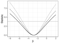
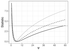
Figure 2: Plot of LR (dotted), mean BRPL (dashed) and median BRPL (solid) ratio statistic in (7) when $\tau$ is $\beta$ (left) and $\psi$ (right). The horizontal line is the $95\%$ quantile of the limiting $\chi^{2}_{1}$ distribution, and its intersection with the values of the statistics results in the endpoints of the corresponding $95\%$ confidence intervals.

In order to further investigate the performance of the three approaches to estimation and inference, we performed a simulation study where we simulated $10\,000$ independent samples from the random-effects meta-analysis model with parameter values set to the ML estimates reported earlier, i.e. $\beta_{0}=-2.799$ and $\psi_{0}=4.199$. Figure 3 shows boxplots of the estimates of $\beta$ and $\psi$ calculated from each of the $10\,000$ simulated samples. The distributions of the three alternative estimators for $\beta$ are similar. On the other hand, the ML estimator of $\psi$ has a large negative mean bias, maximum median BRPL tends to over-correct for that bias, while maximum mean BRPL almost fully corrects for the bias of ML estimator. The distribution of the median BRPL estimates has the heaviest right tail. The simulation-based estimates of the probabilities of underestimation for $\psi$, $P_{\psi_{0}}(\hat{\psi}\leq\psi_{0})$, $P_{\psi_{0}}(\hat{\psi}^{\ast}\leq\psi_{0})$ and $P_{\psi_{0}}(\hat{\psi}^{\dagger}\leq\psi_{0})$ are 0.708, 0.591 and 0.493 for the ML, maximum mean BRPL, and maximum median BRPL, respectively, illustrating how effective maximizing the median BRPL in (6) is in reducing the median bias of the maximum likelihood estimator of $\psi$.

The simulated samples were also used to calculate the empirical $p$-value distribution for the two-sided tests that each parameter is equal to the true values based on the LR statistic, the mean BRPL ratio statistic, and the median BRPL ratio statistic. Table 1 shows that the empirical $p$-value distribution for the mean and median BRPL ratio statistics are closest to uniformity, with the latter being slightly more conservative than the former. The coverage probability of the $95\%$ confidence intervals of $\beta$ based on the mean BRPL ratio and the median BRPL ratio are notably closer to the nominal level than those based on the likelihood ratio. Specifically, the coverage probabilities for $\beta$ are $88\%$, $93\%$, and $96\%$ for LR, mean BRPL ratio, and median BRPL ratio respectively, and the corresponding coverage probabilities for $\psi$ are $88\%$, $94\%$, and $96\%$, respectively.

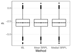
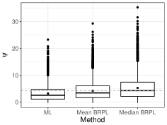
Figure 3: Boxplots for the ML, the maximum mean BRPL, and the maximum median BRPL estimates of $\beta$ and $\psi$ as calculated from $10\,000$ simulated samples under the ML fit using the cocoa data (Bellio & Guolo, 2016; Taubert et al., 2007). The square point is the empirical mean of the estimates. The dashed grey horizontal line is at the parameter value used to generate the data.

Table 1: Empirical $p$-value distribution (%) for the tests based on the LR statistic, the mean BRPL ratio statistic, and the median BRPL ratio statistic in the cocoa data (Bellio & Guolo, 2016; Taubert et al., 2007) setting.

$\alpha\times 100$	$1.0$	$2.5$	$5.0$	$10.0$	$25.0$	$50.0$	$75.0$	$90.0$	$95.0$	$97.5$	$99.0$
LR	5.7	8.4	11.8	18.2	34.6	57.8	79.2	91.8	96.1	98.0	99.3
Mean BRPL ratio	1.6	3.7	6.7	12.2	28.4	52.8	76.6	90.9	95.5	97.9	99.1
Median BRPL ratio	0.6	1.8	4.1	8.6	23.1	48.5	74.2	90.0	95.0	97.5	99.1

6 Simulation study

More extensive simulations under the random-effects meta-analysis model (1) are performed here using the design in Brockwell & Gordon (2001). Specifically, the data $y_{i}\,$, $i\in\{1,\ldots,K\}$, are simulated from model (1) with true fixed-effect parameter $\beta=0.5$. The within-study variances $\hat{\sigma}^{2}_{i}$ are independently generated from a $\chi^{2}_{1}$ distribution and are multiplied by $0.25$ before restricted to the interval $(0.009,0.6)$. Eleven values of the between-study variance $\psi$ ranging from $0$ to $0.1$ are chosen, and the number of studies $K$ ranges from $5$ to $200$. For each combination of $\psi$ and $K$ considered, we simulated $10\,000$ data sets initializing the random number generator at a common state. The within-study variances where generated only once and kept fixed while generating the samples.

Zeng & Lin (2015) compared the performance of their proposed double resampling method with the DerSimonian & Laird (1986) method, the profile likelihood method in Hardy & Thompson (1996), and the resampling method in Jackson & Bowden (2009) and showed that the double resampling method improves the accuracy of statistical inference. Based on these results Kosmidis et al. (2017) compared the performance of their mean BRPL approach with the double resampling method and illustrated that the former results in confidence intervals with coverage probabilities closer to the nominal level that the alternative methods.

We take advantage of the results reported in Zeng & Lin (2015) and Kosmidis et al. (2017) and evaluate the performance of estimation and inference based only on the median BRPL with that based on the likelihood and the mean BRPL. The estimators of the fixed and random-effect parameters obtained from the three methods are calculated using variants of the two-step algorithm described in Section 4.2. In the second step of the algorithm the candidate values for the ML, and maximum mean and median BRPL estimators of the between-study variance $\psi$ are calculated by searching for the root of the partial derivatives of $l(\theta)$, $l^{\ast}(\theta)$, and $l^{\dagger}(\theta)$ with respect to $\psi$, in the interval $(0,3)$.

First, we compare the performance of the ML, maximum mean BRPL and maximum median BRPL estimators in terms of percentage of underestimation. Figure 4 shows that the median bias-reducing adjustment is the most effective in reducing median bias even for small values of $K$. As expected, the ML and maximum mean BRPL estimators also approach the limit of $50\%$ underestimation as $K$ grows, with the latter being closer to $50\%$ than the former. Figure 5 shows that maximum median BRPL is also effective in reducing the mean bias of the ML estimator of $\psi$ but only for moderate to large values of $K$, while maximum mean BRPL results in estimators with the smallest bias.

Figures 6 and 7 show the estimated coverage probability for the one-sided and two-sided confidence intervals for $\beta$ based on the LR, mean BRPL ratio and median BRPL ratio statistics at the $95\%$ nominal level. Figure 8 shows the estimated coverage probability for the two-sided confidence intervals for $\psi$ based on the LR, mean BRPL ratio and median BRPL ratio statistics at the $95\%$ nominal level. For small values of $\psi$ or small and moderate number of studies $K$ the empirical coverage of the intervals is larger than the nominal $95\%$ level. In general, the confidence intervals based on mean and median BRPL ratio have empirical coverage that is closer to the nominal level with the latter having generally better coverage. The differences between the three methods diminish as the number of studies $K$ increases.

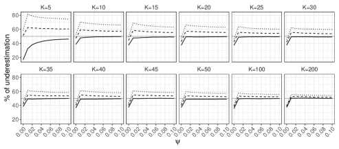
Figure 4: Empirical percentage of underestimation for $\psi$ for random-effects meta-analysis. The percentage of underestimation is calculated for $K\in\{5,10,15,20,25,30,35,40,45,50,100,200\}$ and for increasing values of $\psi$ in the interval $[0,0.1]$. The curves correspond to the maximum median BRPL (solid), maximum mean BRPL (dashed), and ML (dotted) estimators. The grey horizontal line is at the target of 50% underestimation.

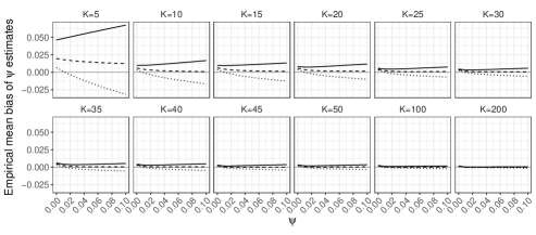
Figure 5: Empirical mean bias of $\psi$ estimates for random-effects meta-analysis. The mean bias is calculated for $K\in\{5,10,15,20,25,30,35,40,45,50,100,200\}$ and for increasing values of $\psi$ in the interval $[0,0.1]$. The curves correspond to the maximum median BRPL (solid), maximum mean BRPL (dashed), and ML (dotted) estimators. The grey horizontal line is at zero.

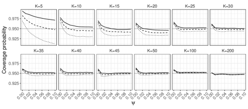
Figure 6: Empirical coverage probabilities of one-sided (right) confidence intervals for $\beta$ for random-effects meta-analysis. The empirical coverage is calculated for increasing values of $\psi$ in the interval $[0,0.1]$ and for $K\in\{5,10,15,20,25,30,35,40,45,50,100,200\}$. The curves correspond to nominally $95\%$ internals based on the median BRPL ratio (solid), the mean BRPL ratio (dashed), and the LR (dotted). The grey horizontal line is at the $95\%$ nominal level.

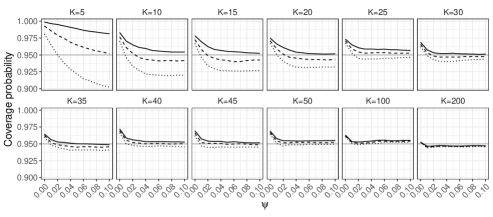
Figure 7: Empirical coverage probabilities of two-sided confidence intervals for $\beta$ for random-effects meta-analysis. The empirical coverage is calculated for increasing values of $\psi$ in the interval $[0,0.1]$ and for $K\in\{5,10,15,20,25,30,35,40,45,50,100,200\}$. The curves correspond to nominally $95\%$ confidence intervals based on the median BRPL ratio (solid), the mean BRPL ratio (dashed), and the LR (dotted). The grey horizontal line is at the $95\%$ nominal level.

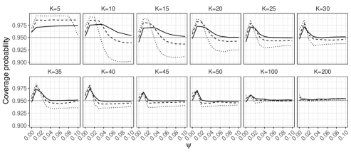
Figure 8: Empirical coverage probabilities of two-sided confidence intervals for $\psi$ for random-effects meta-analysis. The empirical coverage is calculated with $\beta=0.5$ and for increasing values of $\psi$ in the interval $[0,0.1]$ and for $K\in\{5,10,15,20,25,30,35,40,45,50,100,200\}$. The curves correspond to nominally $95\%$ confidence intervals based on the median BRPL ratio (solid), the mean BRPL ratio (dashed), and the LR (dotted). The grey horizontal line is at the $95\%$ nominal level.

Figures 9 and 10 give the power of the LR, the mean BRPL ratio, and the median BRPL ratio tests for testing the null hypothesis $\beta=0.5$ against various alternatives. Specifically, we simulated $10~{}000$ data sets under the alternative hypothesis that parameter $\beta$ is equal to $b=0.5+\delta K^{-1/2}$, where $\delta$ ranges from $0$ to $2.25$. In Figure 9 the power is calculated using critical values of the the asymptotic null $\chi^{2}_{1}$ distribution of the statistics. In Figure 10 the power is calculated using critical values based on the exact null distribution of each statistic, obtained by simulation under the null hypothesis. In this way, the three tests are calibrated to have size $5\%$.

Figure 9 shows that the three tests have monotone power and for small values of $K$ the LR test yields the largest power. This is because the LR test is oversized, while the mean and median BRPL ratio tests are slightly more conservative and this conservativeness comes at the cost of lower power. As the number of studies $K$ increases the three tests approach the nominal size and provide similar power. The use of the exact critical values in Figure 10 allows us to compare the performance of the tests without letting the oversizing or the conservativeness of a test skew the power results. Figure 10 shows that the power of the median BRPL ratio test is almost identical to that of the mean BRPL ratio test, and both tests have larger power than the LR test. Again, inference based on either of the two penalized likelihoods becomes indistinguishable from classical likelihood inference as the number of studies increases.

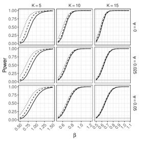
Figure 9: Empirical power of the likelihood-based tests of asymptotic level $0.05$ for random-effects meta-analysis for testing $\beta=0.5$. The empirical power is calculated for increasing values of $\beta$, for $K\in\{5,10,15\}$ and $\psi\in\{0,0.025,0.05\}$. The curves correspond to median BRPL ratio (solid), mean BRPL ratio (dashed), and LR (dotted) tests. The grey horizontal line is at the $5\%$ nominal size.

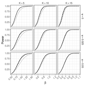
Figure 10: Empirical power of the likelihood-based tests of exact level $0.05$ for random-effects meta-analysis for testing $\beta=0.5$. The empirical power is calculated for increasing values of $\beta$, for $K\in\{5,10,15\}$ and $\psi\in\{0,0.025,0.05\}$. The curves correspond to median BRPL ratio (solid), mean BRPL ratio (dashed), and LR (dotted) tests. The grey horizontal line is at the $5\%$ nominal size.

Across all $\psi$ and $K$ values considered, the average number of iterations taken per fit for the two-step iterative process to converge is 6.20, 5.75 and 5.86 iterations for ML, maximum mean BRPL, and maximum median BRPL, respectively. The average computational run-times for ML, maximum mean BRPL, and maximum median BRPL are 0.005, 0.021, and 0.017 seconds, respectively. Figures 1 and 2 in the Supplementary material show the average number of iterations and the average computational run-time taken per fit for the two-step iterative process to converge for each value of $K$ and $\psi$ used in the simulation study. The results show that in all cases estimation is achieved rapidly and after a small number of iterations for all three methods, with only negligible overhead with the two bias reducing methods.

7 Meat consumption data

Larsson & Orsini (2014) investigate the association between meat consumption and relative risk of all-cause mortality. The data consists of $16$ prospective studies, eight of which are about unprocessed red meat consumption and eight about processed meat consumption. Figure 11 displays the information provided by each study in the meta-analysis. The results from the studies point towards the conclusion that high consumption of red meat, in particular processed red meat, is associated with higher all-cause mortality.

Figure 11: The meat consumption data (Larsson & Orsini, 2014). Outcomes from 16 studies are reported in terms of the logarithm of the relative risk (Log RR) of all-cause mortality for the highest versus lowest category of unprocessed red meat, and processed meat consumption. Squares represent the mean effect estimate for each study; the size of the square reflects the weight that the corresponding study exerts in the meta-analysis. Horizontal lines represent $95\%$ Wald-type confidence intervals (CI) of the effect estimate of individual studies.

We consider the random-effects meta-regression model, assuming that $Y_{i}$ has a $N(\beta_{0}+\beta_{1}x_{i},\hat{\sigma}^{2}_{i}+\psi)$, where $Y_{i}$ is the random variable representing the logarithm of the relative risk reported in the $i$th study, and $x_{i}$ takes value $1$ if the consumption in the $i$th study is about processed red meat and $0$ if it is about unprocessed meat $(i=1,\ldots,16)$. Table 2 gives the ML estimates, the mean BRPL estimates, and the median BRPL estimates of $\beta_{0}$, $\beta_{1}$ and $\psi$, along with the corresponding standard errors for $\beta_{0}$ and $\beta_{1}$. The median BRPL estimate of $\psi$ and the standard errors of the fixed-effect parameters are the largest. The iterative process for computing the ML, maximum mean BRPL, and maximum median BRPL estimates converged in eight, nine, and twelve iterations, in $1.2\times 10^{-2}$, $2.4\times 10^{-2}$, and $1.5\times 10^{-2}$ seconds, respectively.

The LR test indicates some evidence for a higher risk associated to the consumption of red processed meat with a $p$-value of $0.047$. On the other hand, the mean and median BRPL ratio tests suggest that there is weaker evidence for higher risk, with $p$-values of $0.066$ and $0.074$, respectively. Skovgaard’s test also gives weak evidence for higher risk with $p$-value 0.073.

Table 2: ML, maximum mean BRPL, and maximum median BRPL estimates of the model parameters for the meat consumption data (Larsson & Orsini, 2014). Standard errors are reported in parentheses. The $95\%$ confidence intervals based on the LR, mean BRPL ratio and median BRPL ratio are reported in squared brackets.

Method	$\beta_{0}$	$\beta_{1}$	$\psi$
ML	0.099 (0.044)	0.106 (0.061)	0.009
	[-0.004,0.189]	[-0.022,0.244]	[0.003,0.030]
Maximum mean BRPL	0.095 (0.050)	0.110 (0.069)	0.012
	[-0.020,0.199]	[-0.040,0.264]	[0.003,0.042]
Maximum median BRPL	0.093 (0.052)	0.111 (0.072)	0.013
	[-0.027,0.203]	[-0.048,0.271]	[0.004,0.048]

Similar to Section 5, we performed a simulation study in order to further investigate the performance of the three methods in a meta-regression context. We simulated $10\,000$ independent samples from the meta-regression model at the ML estimates reported in Table 2. Figure 12 shows boxplots of the estimates of $\beta_{0}$, $\beta_{1}$, and $\psi$. Maximum likelihood underestimates the parameter $\psi$, while mean BRPL and median BRPL almost fully compensate for the negative bias of ML estimates, with the latter having a slightly heavier right tail. The percentages of underestimation are $72.6\%$, $56.6\%$, and $49.9\%$ for the ML, maximum mean BRPL, and maximum median BRPL estimators, respectively.

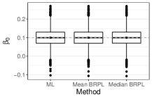
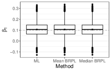
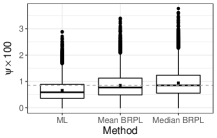
Figure 12: Boxplots for the ML, maximum mean BRPL, and maximum median BRPL estimates of $\beta_{0}$, $\beta_{1}$, and $\psi$ as calculated from $10\,000$ simulated samples under the ML fit using the meat consumption data (Larsson & Orsini, 2014). The square point is the mean of the estimates obtained from each method. The dashed grey horizontal line is at the parameter value used to generate the data.

The simulated samples were also used to calculate the empirical $p$-value distribution for the tests based on the likelihood, mean BRPL and median BRPL ratio statistics. Table 3 shows that the empirical $p$-value distribution for the median BRPL ratio statistic is the one closest to uniformity.

Table 3: Empirical $p$-value distribution (%) for the tests based on the LR statistic, the mean BRPL ratio statistic, and the median BRPL ratio ratio statistic using the meat consumption data (Larsson & Orsini, 2014).

$\alpha\times 100$	$1.0$	$2.5$	$5.0$	$10.0$	$25.0$	$50.0$	$75.0$	$90.0$	$95.0$	$97.5$	$99.0$
LR	2.2	4.5	7.7	13.1	28.0	50.0	71.7	86.6	92.1	95.3	97.7
Mean BRPL ratio	1.3	3.0	5.6	11.1	25.9	49.8	73.8	89.0	94.2	96.9	98.6
Median BRPL ratio	1.0	2.5	4.9	9.9	25.1	49.7	74.7	89.8	94.8	97.5	98.9

8 Concluding remarks

In this paper we derive the adjusted score equations for the median bias reduction of the ML estimator for random-effects meta-analysis and meta-regression models and describe the associated inferential procedures.

We show that the solution of the median bias-reducing adjusted score equations is equivalent to maximizing a penalized log-likelihood. The logarithm of that penalized likelihood differs from the logarithm of the mean BRPL in Kosmidis et al. (2017) by a simple additive term. The computation of the maximum median BRPL estimators can be performed through a two-step iteration that involves a weighted least squares update and the solution of a nonlinear equation with respect to a scalar parameter, and which converges rapidly, as illustrated by the computational times and number of iterations reported in the paper. The reported times and number of iterations were computed using a workstation with 24 cores at 2.90GHz and 80GB memory running under the CentOS 7 operating system, using one core per data set.

Using various settings we were able to retrieve enough information on the performance of the maximum median BRPL estimators. All our simulation studies illustrate that use of the median BRPL succeeds in achieving median centering in estimation, and results in confidence intervals with good coverage properties. Furthermore, while tests based on the LR suffer from size distortions, the median BRPL ratio statistic results in tests with size and power properties, sometimes better to those of the mean BRPL ratio statistic in Kosmidis et al. (2017).

The main advantage of the maximum median BRPL estimators from the maximum mean BRPL ones is their equivariance under monotone component-wise parameter transformations, which, in the case of random-effects meta-regression, leads to median bias-reduced standard errors.

As random-effect models are widely used in practice, the median BRPL method is likely to be useful in models with more complex random-effect structures, such as linear mixed models.

Supplementary material

The R code for replication of examples is provided as online supplementary material.

Funding

The first author was partially supported by the Erasmus+ programme of the European Union which funded her for a 2-month traineeship at the University of Padova. The work of the second author was supported by the Alan Turing Institute under the EPSRC grant EP/N510129/1 (Turing award number TU/B/000082) and part of it was completed when he was a Senior Lecturer at University College London. The third author was supported by the Italian Ministry of Education under the PRIN 2015 grant 2015EASZFS_003, and by the University of Padova (PRAT 2015).

Appendix

The observed information matrix for the random-effects meta-regression model (1) is

$$j(\theta)=\begin{pmatrix}X^{{\mathrm{\scriptscriptstyle T}}}W(\psi)X&X^{{\mathrm{\scriptscriptstyle T}}}W(\psi)^{2}R(\beta)\\ X^{{\mathrm{\scriptscriptstyle T}}}W(\psi)^{2}R(\beta)&R(\beta)^{{\mathrm{\scriptscriptstyle T}}}W(\psi)^{3}R(\beta)-\frac{1}{2}\operatorname{tr}[W(\psi)^{2}]\end{pmatrix}.$$

For this model

$$P_{t}(\theta)=-Q_{t}(\theta)=\begin{pmatrix}0_{p\times p}&X^{{\mathrm{\scriptscriptstyle T}}}W(\psi)^{2}X_{t}\\ X^{{\mathrm{\scriptscriptstyle T}}}W(\psi)^{2}X_{t}&0\end{pmatrix}\quad(t=1,\ldots,p)\,,$$

and

$$P_{p+1}(\theta)=\begin{pmatrix}X^{{\mathrm{\scriptscriptstyle T}}}W(\psi)^{2}X&0_{p}\\ 0_{p}^{{\mathrm{\scriptscriptstyle T}}}&\operatorname{tr}(W(\psi)^{3})\end{pmatrix}~{}~{}~{}\text{ and }~{}~{}~{}Q_{p+1}(\theta)=\begin{pmatrix}0_{p\times p}&0_{p}\\ 0_{p}^{{\mathrm{\scriptscriptstyle T}}}&-\operatorname{tr}(W(\psi)^{3})\end{pmatrix}\,,$$

where $0_{p\times p}$ is the $p\times p$ zero matrix and $X_{t}$ is the $t$th column of $X$. The median bias-reducing adjustment for $\theta$ is obtained by plugging the above expressions into (4). The sum $P_{t}(\theta)+Q_{t}(\theta)$ ($t=1,\ldots,p+1$) is also given in the Appendix of Kosmidis et al. (2017).

See pages 1-8 of Suppl_KKS.pdf

References

- Bellio & Guolo (2016) Bellio R and Guolo A. Integrated likelihood inference in small sample meta-analysis for continuous outcomes. Scand. J. Stat. 2016; 43: 191–201.
- Brockwell & Gordon (2001) Brockwell SE and Gordon IR. A comparison of statistical methods for meta-analysis. Stat. Med. 2001; 20: 825–840.
- DerSimonian & Laird (1986) DerSimonian R and Laird N. Meta-analysis in clinical trials. Control. Clin. Trials 1986; 7: 177–188.
- Firth (1993) Firth D. Bias reduction of maximum likelihood estimates. Biometrika 1993; 80: 27–38.
- Guolo & Varin (2015) Guolo A and Varin C. Random-effects meta-analysis: The number of studies matters. Stat. Methods Med. Res. 2017; 26: 1500–1518.
- Hardy & Thompson (1996) Hardy RJ and Thompson SG. A likelihood approach to meta-analysis with random effects. Stat. Med. 1996; 15: 619–629.
- Huizenga et al. (2011) Huizenga HM, Visser i and Dolan CV. Testing overall and moderator effects in random effects meta-regression. Br. J. Math. Stat. Psychol. 2011; 64: 1–19.
- Jackson & Bowden (2009) Jackson D and Bowden J. A re-evaluation of the “quantile approximation method” for random effects meta-analysis. Stat. Med. 2009; 28: 338–348.
- Kenne Pagui et al. (2016) Kenne Pagui EC, Salvan A and Sartori N. Median bias reduction of maximum likelihood estimates. Biometrika 2017; 104: 923–938.
- Knapp & Hartung (2003) Knapp G and Hartung J. Improved tests for a random effects meta-regression with a single covariate. Stat. Med. 2003; 22: 2693–2710.
- Kosmidis & Firth (2009) Kosmidis I and Firth D. Bias reduction in exponential family nonlinear models. Biometrika 2009; 96: 793–804.
- Kosmidis et al. (2017) Kosmidis I, Guolo A and Varin C. Improving the accuracy of likelihood-based inference in meta-analysis and meta-regression. Biometrika 2017; 104: 489–496.
- Larsson & Orsini (2014) Larsson SC and Orsini N. Red meat and processed meat consumption and all-cause mortality: A meta-analysis. Am. J. Epidemiol. 2014; 179: 282–289.
- Pace & Salvan (1997) Pace L and Salvan A. Principles of statistical inference: From a neo-Fisherian perspective. 1997; London: World Scientific.
- Taubert et al. (2007) Taubert D, Roesen R and Schömig E. Effect of cocoa and tea intake on blood pressure: a meta-analysis. Arch. Intern. Med. 2007; 167: 626–634.
- Van Houwelingen et al. (2002) Van Houwelingen HC, Arends LR and Stijnen T. Advanced methods in meta-analysis: multivariate approach and meta-regression. Stat. Med. 2002; 21: 589–624.
- Zeng & Lin (2015) Zeng D and Lin DY. On random-effects meta-analysis. Biometrika 2015; 102: 281–294.