Effective-range function methods for charged particle collisions

Abstract

Different versions of the effective-range function method for charged particle collisions are studied and compared. In addition, a novel derivation of the standard effective-range function is presented from the analysis of Coulomb wave functions in the complex plane of the energy. The recently proposed effective-range function denoted as $\displaystyle\Delta_{\ell}$ [Phys. Rev. C 96, 034601 (2017)] and an earlier variant [Hamilton et al., Nucl. Phys. B 60, 443 (1973)] are related to the standard function. The potential interest of $\displaystyle\Delta_{\ell}$ for the study of low-energy cross sections and weakly bound states is discussed in the framework of the proton-proton $\displaystyle{}^{1}S_{0}$ collision. The resonant state of the proton-proton collision is successfully computed from the extrapolation of $\displaystyle\Delta_{\ell}$ instead of the standard function. It is shown that interpolating $\displaystyle\Delta_{\ell}$ can lead to useful extrapolation to negative energies, provided scattering data are known below one nuclear Rydberg energy ($\displaystyle 12.5~{}\mathrm{keV}$ for the proton-proton system). This property is due to the connection between $\displaystyle\Delta_{\ell}$ and the effective-range function by Hamilton et al. that is discussed in detail. Nevertheless, such extrapolations to negative energies should be used with caution because $\displaystyle\Delta_{\ell}$ is not analytic at zero energy. The expected analytic properties of the main functions are verified in the complex energy plane by graphical color-based representations.

I Introduction

In quantum collision theory, the effective-range function (ERF) method is a powerful model-independent fitting technique of low-energy phase shifts Bethe (1949); Landau and Smorodinsky (1944); Blatt (1948); Chew and Goldberger (1949); Jackson and Blatt (1950); Joachain (1979); Newton (1982); van Haeringen (1985). It is very useful in nuclear collision physics when the shape of the interaction potentials is not known accurately. This method merely consists in expanding a function of the phase shift, namely the ERF, that is analytic at zero energy and behaves as a constant at this point Bethe (1949). The expansion of the ERF — also referred to as the effective-range expansion — can be either a power series of the energy or a Padé approximant, i.e., a rational function. In general, Padé approximants are valid on a larger domain than Taylor series Hartt (1981); Rakityansky and Elander (2013); Midya et al. (2015).

The ERF method was mainly developed in the 1940s by Schwinger, Bethe Bethe (1949), Landau Landau and Smorodinsky (1944), and others in the framework of nucleon-nucleon collisions. In these works, it is shown that the ERF specifically dedicated to charged particle scattering is very different from the one of neutral particle scattering because of the Coulomb interaction. In particular, the Coulomb interaction modifies the low-energy behavior of the phase shift, involving a special analytical structure described by the digamma function Bethe (1949); Abramowitz and Stegun (1964); Olver et al. (2010). Since then, the ERF for charged particle scattering has been the subject of many developments Cornille and Martin (1962); Lambert (1969); Hamilton et al. (1973); van Haeringen and Kok (1982); Humblet (1990); Yarmukhamedov and Baye (2011); Rakityansky and Elander (2013); Ramírez Suárez and Sparenberg (2017); Blokhintsev et al. (2017a, b); Orlov et al. (2016, 2017). Moreover, the method has been applied to experimental data of numerous two-body systems, such as: proton-proton Bethe (1949); Landau and Smorodinsky (1944); Blatt (1948); Chew and Goldberger (1949); Jackson and Blatt (1950); Naisse (1977); Kok (1980); Hartt (1981); Bergervoet et al. (1988); Mukhamedzhanov et al. (2010), proton-deuteron Chen et al. (1989); Kievsky et al. (1997); Brune et al. (2001), or $\displaystyle{}^{12}\mathrm{C}+\alpha$ Humblet et al. (1976); Brune et al. (1999); Filippone et al. (1989); Ramírez Suárez and Sparenberg (2017); Blokhintsev et al. (2017a, b); Orlov et al. (2016, 2017).

However, this ERF also raises technical issues related to the relative magnitude of its digamma function term versus the phase-shift-dependent term. According to recent works Ramírez Suárez and Sparenberg (2017); Blokhintsev et al. (2017a, b), it would be less appropriate to model the phase shift for heavier nuclei than protons. In Ref. Ramírez Suárez and Sparenberg (2017), it is suggested to use a reduced variant of the ERF — that is denoted as $\displaystyle\Delta_{\ell}$ — as a potential alternative to the standard Coulomb-modified ERF for studying the weakly bound states by extrapolation of scattering data to negative energies. This reduced ERF method is also inspired by earlier works Hamilton et al. (1973); Humblet (1990) about the mathematical properties of the standard ERF.

The main purpose of this paper is to study the reduced ERF method Ramírez Suárez and Sparenberg (2017) and to clarify its connection to the standard ERF method. In addition, we propose a novel derivation of the standard ERF as well as the relations between the different historical formulations.

We show that the reduced ERF method allows us to obtain information on resonances and weakly bound states, using the properties of the digamma function appearing in the standard ERF. These properties are graphically verified in the complex plane of the energy $\displaystyle E$. Indeed, complex plots have the advantage of revealing the analytic structures that are concealed from the real $\displaystyle E$-axis. This leads to predictions on the singularities of the Coulomb phase shift.

Finally, we apply the reduced ERF method to the proton-proton $\displaystyle{}^{1}S_{0}$ collision to check the predictions of the effective-range theory. We show that the singular nature of $\displaystyle\Delta_{\ell}$ at negative energy prevents Padé approximants from converging below $\displaystyle E=0$. However, depending on the energy range covered by experimental data, it seems possible with $\displaystyle\Delta_{\ell}$ to extrapolate to negative energy up to about minus one nuclear Rydberg, using the connection between the reduced ERF and the ERF by Hamilton et al. Hamilton et al. (1973), that we denote as $\displaystyle\Delta^{+}_{\ell}$.

This paper is organized as follows: Section II provides the derivation of the analytic structure of the Coulomb wave functions in the complex $\displaystyle E$-plane. Thereafter, the calculation of the ERFs and the study of their properties in the complex $\displaystyle E$-plane are presented in Section III. This analysis is performed by explicit calculation and is aided by graphics in the complex plane. We focus on the properties of $\displaystyle\Delta_{\ell}$ and $\displaystyle\Delta^{+}_{\ell}$. Section IV describes the theoretical properties of the ERFs in the framework of the proton-proton $\displaystyle{}^{1}S_{0}$ collision. We also study the ability of the reduced ERF $\displaystyle\Delta_{\ell}$ to extrapolate data to negative energies.

Throughout the text, we use the reduced Planck constant $\displaystyle\hbar c$, the fine-structure constant $\displaystyle\alpha$ and the rest mass energy of the proton $\displaystyle m_{\mathrm{p}}c^{2}$ provided by the 2014 CODATA recommended values Mohr et al. (2016).

II Pure Coulomb potential

This section deals with the theoretical aspects of the non-relativistic scattering of two charged particles, especially in the low-energy limit. The Coulomb wave functions are analyzed in the complex plane of the energy.

II.1 Scattering wave functions in Coulomb potential

The effective-range theory of the Coulomb scattering is largely based on the analytic expression of the solutions of the Schrödinger equation in a $\displaystyle 1/r$-potential. Indeed, the Coulomb wave functions are involved in the very definition of the phase shift Breit et al. (1936); Bethe (1949); Landau and Smorodinsky (1944); Blatt (1948); Chew and Goldberger (1949); Jackson and Blatt (1950); Messiah (1961); Gottfried (1966); Joachain (1979); van Haeringen (1985); Newton (1982); Humblet (1990); Rakityansky and Elander (2013).

We consider two spinless particles of negligible radius, respective masses $\displaystyle m_{1}$ and $\displaystyle m_{2}$, and charges $\displaystyle Z_{1}e$ and $\displaystyle Z_{2}e$. If $\displaystyle\mathbf{r}$ denotes the relative position between the particles and $\displaystyle E=\hbar^{2}k^{2}/2m$ the energy in the center-of-mass frame, the Schrödinger equation writes Messiah (1961); Gottfried (1966)

$$-\frac{\hbar^{2}}{2m}\nabla^{2}\Psi(\mathbf{r})+\frac{Z_{1}Z_{2}e^{2}}{4\pi\epsilon_{0}\,r}\Psi(\mathbf{r})=\frac{\hbar^{2}k^{2}}{2m}\Psi(\mathbf{r})\>,$$ (1)

where $\displaystyle m=m_{1}m_{2}/(m_{1}+m_{2})$ is the reduced mass of the two-body system. Since the Coulomb potential is isotropic — it only depends on $\displaystyle r=\left\|\mathbf{r}\right\|$ —, the angular momentum commutes with the Hamiltonian. If, in addition, we focus on a partial wave of specific angular momentum, the wave function $\displaystyle\Psi(\mathbf{r})$ splits into an angular part given by spherical harmonics $\displaystyle Y_{\ell m}(\theta,\phi)$ and a radial part $\displaystyle u_{k\ell}(r)$ to be determined Messiah (1961); Joachain (1979),

$$\Psi_{k\ell m}(\mathbf{r})=\frac{u_{k\ell}(r)}{r}Y_{\ell m}(\theta,\phi)\>.$$ (2)

Replacing (2) in (1) and using the reduced radial coordinate $\displaystyle x=kr$, the Schrödinger equation (1) for $\displaystyle u=u_{k\ell}(r)$ becomes

$$-\frac{\mathop{}\!\mathrm{d}^{2}u}{\mathop{}\!\mathrm{d}x^{2}}+\left[\frac{\ell(\ell+1)}{x^{2}}+\frac{2\eta}{x}-1\right]u=0\>,$$ (3)

also known as the Coulomb wave equation Bateman et al. (1953); Abramowitz and Stegun (1964); Olver et al. (2010). The strength of the Coulomb interaction is determined by the dimensionless Sommerfeld parameter $\displaystyle\eta$ defined as

$$\eta=\frac{\alpha Z_{1}Z_{2}mc^{2}}{\hbar c\,k}=\frac{1}{a_{\mathrm{B}}k}\>,$$ (4)

where $\displaystyle a_{\mathrm{B}}$ stands for the nuclear Bohr radius (in unit length)

$$a_{\mathrm{B}}=\frac{\hbar c}{\alpha Z_{1}Z_{2}mc^{2}}\>.$$ (5)

The nuclear Bohr radius of a two-proton system is $\displaystyle a_{\mathrm{B}}=57.64~{}\mathrm{fm}$, which is significantly larger than the one-femtometer charge radius of the proton. Such a large Bohr radius is due to the relatively small charge and mass of the proton compared to heavier ions. For instance, the nuclear Bohr radius of a $\displaystyle{}^{12}\mathrm{C}+\alpha$ system is barely $\displaystyle 0.806~{}\mathrm{fm}$, i.e., nearly a hundred times smaller. This disparity for proton-proton scattering will play a key role in Sec. IV Bethe (1949).

We also define the nuclear Rydberg energy as

$$1~{}\mathrm{Ry}=\frac{\hbar^{2}}{2ma_{\mathrm{B}}^{2}}=\frac{1}{2}(\alpha Z_{1}Z_{2})^{2}mc^{2}\>,$$ (6)

which equals $\displaystyle 12.49~{}\mathrm{keV}$ for a two-proton system and $\displaystyle 10.72~{}\mathrm{MeV}$ for ${}^{12}\mathrm{C}+\alpha$.

It is well known in the literature that Eq. (3) is solved by the Coulomb wave functions Breit et al. (1936); Bethe (1949); Landau and Smorodinsky (1944); Blatt (1948); Chew and Goldberger (1949); Jackson and Blatt (1950); Bateman et al. (1953); Messiah (1961); Gottfried (1966); Joachain (1979); van Haeringen (1985); Newton (1982); Abramowitz and Stegun (1964); Olver et al. (2010); Humblet (1984); Yost et al. (1936). In this paper, we focus on two useful couples of linearly independent solutions of Eq. (3): $\displaystyle\{F_{\eta\ell}(x),G_{\eta\ell}(x)\}$ and $\displaystyle\{H^{+}_{\eta\ell}(x),H^{-}_{\eta\ell}(x)\}$. The first couple consists of the regular Coulomb function $\displaystyle F_{\eta\ell}(x)$ and the irregular Coulomb function $\displaystyle G_{\eta\ell}(x)$. These functions are so called because of their behavior near the origin ($\displaystyle x=0$): the former goes like $\displaystyle x^{\ell+1}$ and the latter like $\displaystyle x^{-\ell}$ for $\displaystyle x\rightarrow 0$ Abramowitz and Stegun (1964); Olver et al. (2010).

The regular Coulomb function $\displaystyle F_{\eta\ell}(x)$ is defined from the confluent hypergeometric function ${}_{1}F_{1}(a,b,z)$, also known as the Kummer function $\displaystyle M(a,b,z)$ Kummer (1837); Abramowitz and Stegun (1964); Olver et al. (2010)

$$\begin{split}M(a,b,z)&=1+\frac{a}{b}\frac{z}{1!}+\frac{a(a+1)}{b(b+1)}\frac{z^{2}}{2!}+\ldots\\ &=\sum_{n=0}^{\infty}\frac{(a)_{n}}{(b)_{n}}\frac{z^{n}}{n!}\>,\end{split}$$ (7)

where $\displaystyle(a)_{n}=a(a+1)\cdots(a+n-1)=\Gamma(a+n)/\Gamma(a)$ denotes the Pochammer symbol. The regular Coulomb function reads Abramowitz and Stegun (1964); Olver et al. (2010)

$$F_{\eta\ell}(x)=C_{\eta\ell}\,x^{\ell+1}\mathop{}\!\mathrm{e}^{\mathrm{i}x}M(\ell+1+\mathrm{i}\eta,2\ell+2,-2\mathrm{i}x)\>.$$ (8)

It should be noted that, since $\displaystyle k$ appears in $\displaystyle\eta=1/a_{\mathrm{B}}k$ in addition to $\displaystyle x=kr$, the wave number $\displaystyle k$ does not only act on the radial scale of the Coulomb wave functions through $\displaystyle x$, but it also affects the wave oscillations through $\displaystyle\eta$, especially for $\displaystyle x\lesssim 1$.

In the definition (8), the normalization coefficient $\displaystyle C_{\eta\ell}$ ensures the far-field behavior

$$F_{\eta\ell}(x)\xrightarrow{x\rightarrow\infty}\sin\left(x-\ell\frac{\pi}{2}-\eta\ln(2x)+\sigma_{\eta\ell}\right)\>,$$ (9)

where $\displaystyle\sigma_{\eta\ell}$ is the pure Coulomb phase shift Abramowitz and Stegun (1964); Olver et al. (2010); Yost et al. (1936); Humblet (1984)

$$\sigma_{\eta\ell}=\arg\Gamma(\ell+1+\mathrm{i}\eta)\>.$$ (10)

The coefficient $\displaystyle C_{\eta\ell}$ turns out to be energy-dependent Abramowitz and Stegun (1964); Olver et al. (2010),

$$C_{\eta\ell}=\frac{2^{\ell}\left|\Gamma(\ell+1+\mathrm{i}\eta)\right|}{(2\ell+1)!\mathop{}\!\mathrm{e}^{\eta\pi/2}}\quad\textrm{for}~{}\eta\in\mathbb{R}\>.$$ (11)

Here, we have to highlight that Eq. (11) is not analytic anywhere in the complex $\displaystyle k$-plane because of the absolute value. The analytic continuation of $\displaystyle C_{\eta\ell}$ to the complex $\displaystyle k$-plane is obtained by replacing $\displaystyle\left|\Gamma(\ell+1+\mathrm{i}\eta)\right|$ by $\displaystyle[\Gamma(\ell+1+\mathrm{i}\eta)\Gamma(\ell+1-\mathrm{i}\eta)]^{1/2}$ as shown in Refs. Lambert (1969); Humblet (1984) and then rewriting the product by means of Euler’s reflection formula Abramowitz and Stegun (1964); Olver et al. (2010)

$$\Gamma(1-z)\,\Gamma(1+z)=\frac{\pi z}{\sin(\pi z)}\>.$$ (12)

The resulting expression

$$C_{\eta\ell}=\frac{(2\eta)^{\ell}}{(2\ell+1)!}\sqrt{\frac{2\eta\pi w_{\eta\ell}}{\mathop{}\!\mathrm{e}^{2\eta\pi}-1}}$$ (13)

is analytic in the complex $\displaystyle k$-plane — except for poles and branch cuts — and reduces to Eq. (11) at positive energy. In Eq. (13), $\displaystyle w_{\eta\ell}$ is a polynomial of $\displaystyle(a_{\mathrm{B}}k)^{2}$ defined by

$$w_{\eta\ell}=\prod_{j=0}^{\ell}\left(1+\frac{j^{2}}{\eta^{2}}\right)\>,$$ (14)

which equals $\displaystyle 1$ in the zero-energy limit, as well as for $\displaystyle\ell=0$. The procedure is required to make the Coulomb wave functions analytic in the energy plane. This is an important ingredient of the derivation of the Coulomb-modified ERF.

Before talking about the irregular Coulomb function $\displaystyle G_{\eta\ell}(x)$, we have to introduce the incoming and outgoing Coulomb wave functions, respectively denoted as $\displaystyle H^{-}_{\eta\ell}(x)$ and $\displaystyle H^{+}_{\eta\ell}(x)$. They are defined in a very similar way to Eq. (8) by

$$H^{\pm}_{\eta\ell}(x)=D^{\pm}_{\eta\ell}\,x^{\ell+1}\mathop{}\!\mathrm{e}^{\pm\mathrm{i}x}U(\ell+1\pm\mathrm{i}\eta,2\ell+2,\mp 2\mathrm{i}x)\>,$$ (15)

where $\displaystyle U(a,b,z)$ is the confluent hypergeometric function of the second kind, also known as Tricomi’s function, which is linearly independent of $\displaystyle M(a,b,z)$ Bateman et al. (1953); Abramowitz and Stegun (1964); Olver et al. (2010). The Tricomi function in Eq. (15) is defined by a peculiar series representation. Because $\displaystyle b$ is an integer, $\displaystyle U(a,b,z)$ splits into two parts Olver et al. (2010) that we call $\displaystyle P(a,b,z)$ and $\displaystyle L(a,b,z)$

$$U(a,b,z)=P(a,b,z)+L(a,b,z)\quad\text{for}~{}b\in\mathbb{Z}^{+}\>.$$ (16)

In the following, we occasionally use the symbols $\displaystyle a=\ell+1+\mathrm{i}\eta$, $\displaystyle b=2\ell+2$ and $\displaystyle z=-2\mathrm{i}kr$ borrowed from confluent hypergeometric functions Olver et al. (2010) to shorten the notations of the Coulomb wave functions. In Eq. (16), the first term is a polynomial of negative powers of $\displaystyle z$ Olver et al. (2010)

$$P(a,b,z)=\frac{(2\ell)!}{\Gamma(\ell+1+\mathrm{i}\eta)}\sum_{n=0}^{2\ell}\frac{(-\ell+\mathrm{i}\eta)_{n}}{(-2\ell)_{n}}\frac{z^{n-2\ell-1}}{n!}\>,$$ (17)

and the second one is a generalized series involving logarithmic terms in $\displaystyle z$ Olver et al. (2010)

$$\begin{split}L(a,b,z)&=\frac{(-1)^{2\ell+2}}{(2\ell+1)!\,\Gamma(-\ell+\mathrm{i}\eta)}\sum_{n=0}^{\infty}\frac{(a)_{n}}{(b)_{n}}\frac{z^{n}}{n!}\\ \times&\big{[}\ln z+\psi(a+n)-\psi(b+n)-\psi(n+1)\big{]}\>,\end{split}$$ (18)

where $\displaystyle\psi(z)$ is the digamma function — also known as the psi function — defined as the logarithmic derivative of the gamma function

$$\psi(z)=\Gamma^{\prime}(z)/\Gamma(z)\>.$$ (19)

The function $\displaystyle\psi(z)$ is shown in the complex $\displaystyle z$-plane in Fig. 1(a). One notices the array of poles and zeroes on the negative real $\displaystyle z$-axis; they play an important role in the following.

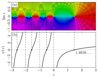
Figure 1: (Color online) Representations of the digamma function $\displaystyle\psi$ (a) in the complex $\displaystyle z$-plane and (b) along the real $\displaystyle z$-axis. Crosses and circles represent poles and zeroes respectively. The color legend is described in Appendix A. The poles occur when $\displaystyle z$ reaches a negative integer or zero. The unique zero on the positive real axis lies at $\displaystyle z=1.4616\ldots$ Olver et al. (2010).

The normalization coefficients $\displaystyle D^{\pm}_{\eta\ell}$ in Eq. (15), that we define as

$$D^{\pm}_{\eta\ell}=\mp 2\mathrm{i}(-1)^{\ell}\mathop{}\!\mathrm{e}^{\eta\pi}\frac{(2\ell+1)!\,C_{\eta\ell}}{\Gamma(\ell+1\mp\mathrm{i}\eta)}\>,$$ (20)

are intended to ensure the asymptotic behavior

$$H^{\pm}_{\eta\ell}(x)\xrightarrow{x\rightarrow\infty}\exp\left\{\pm\mathrm{i}\left[x-\ell\frac{\pi}{2}-\eta\ln(2x)+\sigma_{\eta\ell}\right]\right\}\>.$$ (21)

There are other ways to define $\displaystyle D^{\pm}_{\eta\ell}$ in the literature Yost et al. (1936); Abramowitz and Stegun (1964); Olver et al. (2010); Humblet (1984), but Eq. (20) has the advantage of being proportional to $\displaystyle C_{\eta\ell}$. It will play an important role in Sec. II.2.

Although $\displaystyle D^{+}_{\eta\ell}$ and $\displaystyle D^{-}_{\eta\ell}$, as well as $\displaystyle H^{+}_{\eta\ell}(x)$ and $\displaystyle H^{-}_{\eta\ell}(x)$, are related to each other by complex conjugation at real $\displaystyle k$, this no longer holds when $\displaystyle k$ is complex valued. This is because the complex conjugation is not an analytic operation: $\displaystyle\mkern 3.0mu\overline{\mkern-3.0muz}$ cannot be expanded in power series of $\displaystyle z$ for $\displaystyle z\in\mathbb{C}$. However, one can resort to complex conjugation (in the sense of Ref. Hamming (1973)) to relate them for complex-valued $\displaystyle k$

$$\begin{cases}D^{-}_{\eta\ell}=\mkern 3.0mu\overline{\mkern-3.0muD^{+}_{\mkern 3.0mu\overline{\mkern-3.0mu\eta}\ell}}\>,\\ H^{-}_{\eta\ell}(kr)=\mkern 3.0mu\overline{\mkern-3.0muH^{+}_{\mkern 3.0mu\overline{\mkern-3.0mu\eta}\ell}(\mkern 3.0mu\overline{\mkern-3.0muk}r)}\>,\end{cases}$$ (22)

where $\displaystyle\mkern 3.0mu\overline{\mkern-3.0mu\eta}=1/a_{\mathrm{B}}\mkern 3.0mu\overline{\mkern-3.0muk}$. The relations (22) are practically obtained by replacing everywhere $\displaystyle+\mathrm{i}$ by $\displaystyle-\mathrm{i}$, and conversely.

Contrary to $\displaystyle F_{\eta\ell}(x)$, the functions $\displaystyle H^{\pm}_{\eta\ell}(x)$ are complex valued and irregular at $\displaystyle x=0$ like $\displaystyle x^{-\ell}$. However, the regular Coulomb function can be retrieved by subtracting $\displaystyle H^{-}_{\eta\ell}(x)$ from $\displaystyle H^{+}_{\eta\ell}(x)$

$$F_{\eta\ell}(x)=\frac{H^{+}_{\eta\ell}(x)-H^{-}_{\eta\ell}(x)}{2\mathrm{i}}\>,$$ (23)

which reduces for real $\displaystyle k$ to $\displaystyle\operatorname{Im}H^{+}_{\eta\ell}(x)$ and to the sine wave of Eq. (9) consistently with Eq. (21).

Finally, the irregular Coulomb function $\displaystyle G_{\eta\ell}(x)$ is defined as Yost et al. (1936); Messiah (1961); Humblet (1984); Olver et al. (2010)

$$G_{\eta\ell}(x)=\frac{H^{+}_{\eta\ell}(x)+H^{-}_{\eta\ell}(x)}{2}\>.$$ (24)

This definition has to be understood as the real part $\displaystyle\operatorname{Re}H^{\pm}_{\eta\ell}(x)$ only on the real $\displaystyle k$-axis. Otherwise, when $\displaystyle k$ is complex — at negative energies for instance — Eq. (24) should be preferred, being the analytic continuation of $\displaystyle\operatorname{Re}H^{\pm}_{\eta\ell}(x)$.

From Eq. (21), one easily shows that the irregular function $\displaystyle G_{\eta\ell}(x)$ behaves asymptotically like

$$G_{\eta\ell}(x)\xrightarrow{x\rightarrow\infty}\cos\left(x-\ell\frac{\pi}{2}-\eta\ln(2x)+\sigma_{\eta\ell}\right)\>.$$ (25)

It should be noted that the $\displaystyle s$ wave ($\displaystyle\ell=0$) of $\displaystyle G_{\eta\ell}(x)$ shows a peculiarity in the low-range limit $\displaystyle r\rightarrow 0$. Instead of behaving like $\displaystyle\operatorname{\mathcal{O}}(1)$ as predicted by $\displaystyle\operatorname{\mathcal{O}}(x^{-\ell})$, the irregular wave function $\displaystyle G_{\eta 0}(x)$ is exceptionally dominated by a logarithmic term $\displaystyle\operatorname{\mathcal{O}}(x\ln x)$ emanating from the series (18) in $\displaystyle U(a,b,z)$. As will be seen later in Sec. II.2, such logarithmic terms affect the properties of the irregular Coulomb function in the complex $\displaystyle k$-plane, and in this way the effective-range function.

II.2 Analytic structure of Coulomb wave functions

In this section, we propose a new derivation of the analytic structure of the Coulomb wave functions in the complex plane of the energy $\displaystyle E$, especially in the low-energy limit. We show in Sec. III.1 how the structure of the irregular Coulomb functions $\displaystyle H^{\pm}_{\eta\ell}(x)$ and $\displaystyle G_{\eta\ell}(x)$ leads to the standard effective-range function. To this end, it is crucial to study the analytic properties of the Coulomb wave functions, since they are involved in the very definition of the phase shift $\displaystyle\delta_{\ell}(E)$.

For simplicity, we focus our analysis on Coulomb wave functions divided by the normalization factor $\displaystyle C_{\eta\ell}$ of Eq. (13). Indeed, this factor will disappear from the calculation of the phase shift because the wave function $\displaystyle u_{k\ell}(r)$ is defined within a (possibly complex) factor.

Let us begin with the regular Coulomb function $\displaystyle F_{\eta\ell}(x)$. From the definition (8) and the power series (7), one has

$$\frac{F_{\eta\ell}(kr)}{C_{\eta\ell}(kr)^{\ell+1}\mathop{}\!\mathrm{e}^{\mathrm{i}kr}}=\sum_{n=0}^{\infty}\frac{(\ell+1+\mathrm{i}\eta)_{n}}{(2\ell+2)_{n}}\frac{(-2\mathrm{i}kr)^{n}}{n!}\>.$$ (26)

When the wave number $\displaystyle k$ vanishes, $\displaystyle\eta=1/a_{\mathrm{B}}k$ tends to infinity. Fortunately, the Pochammer symbol $\displaystyle(\ell+1+\mathrm{i}\eta)_{n}$ is asymptotic to $\displaystyle(\mathrm{i}\eta)^{n}$. The numerator in the right-hand side of Eq. (26) becomes $\displaystyle(2\eta kr)^{n}=(2r/a_{\mathrm{B}})^{n}$ which no longer depends on $\displaystyle k$. Therefore, the series is well defined at zero energy and behaves as a constant in the neighborhood of $\displaystyle k=0$.

The analytic structure of the irregular Coulomb functions $\displaystyle H_{\eta\ell}^{\pm}(x)$ and $\displaystyle G_{\eta\ell}(x)$ is less obvious than for $\displaystyle F_{\eta\ell}(x)$ but it has important consequences on the ERF. For convenience, we begin the study with the outgoing Coulomb wave function $\displaystyle H^{+}_{\eta\ell}(x)$ instead of $\displaystyle G_{\eta\ell}(x)$. Given Eqs. (22) and (24), all the equations below for $\displaystyle H^{+}_{\eta\ell}(x)$ will impact those for $\displaystyle G_{\eta\ell}(x)$.

Let us begin the analysis of $\displaystyle H^{+}_{\eta\ell}(x)$ in the $\displaystyle k$-plane with $\displaystyle U(a,b,z)$ from Eq. (16). The two functions $\displaystyle P(a,b,z)$ and $\displaystyle L(a,b,z)$ from Eqs. (17) and (18) are singular in the neighborhood of $\displaystyle k=0$, and one needs to regularize both of them in the limit $\displaystyle k\rightarrow 0$.

First, we consider the finite sum $\displaystyle P(a,b,z)$ from Eq. (17). This function is singular at zero energy on the one hand because of the essential singularity at $\displaystyle k=0$ in $\displaystyle\Gamma(\ell+1+\mathrm{i}\eta)^{-1}$ and on the other hand because each term in the series behaves like $\displaystyle k^{-(2\ell+1)}$ as $\displaystyle k\rightarrow 0$. One way to circumvent this issue is to define the regularized function

$$P^{+}_{\eta\ell}(x)=\frac{(2\ell+1)!}{(\mathrm{i}\eta)^{2\ell+1}}\Gamma(\ell+1+\mathrm{i}\eta)\,P(a,b,z)\>,$$ (27)

which is holomorphic for $\displaystyle k\in\mathbb{C}$ due to the compensation of all the singularities.

Regarding the series $\displaystyle L(a,b,z)$ of Eq. (18), three kinds of singularities have to be considered while regularizing Cornille and Martin (1962); Lambert (1969):

1. the essential singularity of $\displaystyle\Gamma(-\ell+\mathrm{i}\eta)^{-1}$ at $\displaystyle k=0$,

2. the branch cut of the principal-valued logarithm $\displaystyle\ln z$ in the series, and

3. the array of poles of the digamma function $\displaystyle\psi(a+n)$ when $\displaystyle a+n\in\{0,-1,-2,\ldots\}$ leading to an accumulation point at $\displaystyle k=0$.

First, the gamma function $\displaystyle\Gamma(-\ell+\mathrm{i}\eta)^{-1}$ can be compensated in the same way as with $\displaystyle P(a,b,z)$. Secondly, the energy dependence of $\displaystyle\ln z$ can be separated from the radial part as

$$\ln(z)=\ln(-2\mathrm{i}kr)=\ln(2r/a_{\mathrm{B}})-\ln(\mathrm{i}\eta)\>.$$ (28)

It should be noted that the above decomposition assumes that the two particles are repelling each other ($\displaystyle a_{\mathrm{B}}>0$). When it is not true, one can choose $\displaystyle\ln(-2\mathrm{i}kr)=\ln(-2r/a_{\mathrm{B}})-\ln(-\mathrm{i}\eta)$ instead without other significant difference in the calculation.

Finally, the most difficult part of the regularization of $\displaystyle H^{+}_{\eta\ell}(x)$ involves the digamma function $\displaystyle\psi(a+n)$ in the series (18). The digamma function $\displaystyle\psi(a+n)$ has infinitely many poles on the imaginary $\displaystyle k$-axis with an accumulation point at zero energy ($\displaystyle k=0$)

$$k\in\left\{\frac{-\mathrm{i}}{(\ell+n+1)a_{\mathrm{B}}},\frac{-\mathrm{i}}{(\ell+n+2)a_{\mathrm{B}}},\ldots,\rightarrow-0\,\mathrm{i}\right\}\>.$$ (29)

Such a structure is not compensated by the zeroes from $\displaystyle(a)_{n}$. Therefore, one has to separate the digamma function $\displaystyle\psi(a+n)$ from the series (18). For this purpose, one uses the property Abramowitz and Stegun (1964); Olver et al. (2010)

$$\psi(a+n)=\psi(a)+\sum_{s=0}^{n-1}\frac{1}{a+s}\>,$$ (30)

to extract from $\displaystyle\psi(a+n)$ the function $\displaystyle\psi(a)$ independent of the summation index $\displaystyle n$, but still with the $\displaystyle k$-dependence.

From this point on, we exploit the close similarity between the series (18) and the Kummer function (7). Indeed, we guess that the index-independent part will contribute to a Kummer function $\displaystyle M(a,b,z)$, that is holomorphic for $\displaystyle k\in\mathbb{C}$ as shown before in (26). Using Eqs. (28) and (30), one gets the analytic decomposition

$$L(a,b,z)=\frac{g_{\ell}^{+}(\eta)\,M(a,b,z)+\sum_{n=0}^{\infty}c_{n}\frac{(a)_{n}}{(b)_{n}}\frac{z^{n}}{n!}}{(2\ell+1)!\,\Gamma(-\ell+\mathrm{i}\eta)}\>,$$ (31)

where $\displaystyle g^{+}_{\ell}(\eta)$ is given by

$$g^{\pm}_{\ell}(\eta)=\psi(\ell+1\pm\mathrm{i}\eta)-\ln(\pm\mathrm{i}\eta)\>.$$ (32)

The coefficients $\displaystyle c_{n}$ of the series in Eq. (31) contain the terms

$$c_{n}=\ln\left(\frac{2r}{a_{\mathrm{B}}}\right)+\sum_{s=0}^{n-1}\frac{1}{a+s}-\psi(b+n)-\psi(n+1)\>,$$ (33)

which remain after the decomposition. Other equivalent decompositions may lead to different functions $\displaystyle g^{\pm}_{\ell}(\eta)$ and coefficients $\displaystyle c_{n}$. The key point is to realize that the hypergeometric-like series in Eq. (31),

$$\sum_{n=0}^{\infty}c_{n}\frac{(a)_{n}}{(b)_{n}}\frac{z^{n}}{n!}\>,$$ (34)

is holomorphic in the $\displaystyle k$-plane due to compensation between the zeroes of $\displaystyle(a)_{n}z^{n}$ and the poles of

$$\sum_{s=0}^{n-1}\frac{1}{a+s}\>,$$ (35)

in the coefficients $\displaystyle c_{n}$ of Eq. (33). Similarly to what has been done before for $\displaystyle P(a,b,z)$, we define a new $\displaystyle k$-holomorphic function

$$L^{+}_{\eta\ell}(x)=\frac{\Gamma(\ell+1+\mathrm{i}\eta)}{(\mathrm{i}\eta)^{2\ell+1}\Gamma(-\ell+\mathrm{i}\eta)}\sum_{n=0}^{\infty}c_{n}\frac{(a)_{n}}{(b)_{n}}\frac{z^{n}}{n!}\>.$$ (36)

The prefactor in Eq. (36) is obtained by multiplying (31) by the same coefficient as $\displaystyle P(a,b,z)$ of Eq. (27). The idea behind this renormalization is to keep $\displaystyle L^{+}_{\eta\ell}(x)$ on the same footing as $\displaystyle P^{+}_{\eta\ell}(x)$. The resulting prefactor in Eq. (36) is also holomorphic in $\displaystyle k$ as evidenced by the corollary of the recurrence property of the gamma function Humblet (1984)

$$\frac{\Gamma(\ell+1+\mathrm{i}\eta)}{(\mathrm{i}\eta)^{2\ell+1}\Gamma(-\ell+\mathrm{i}\eta)}=w_{\eta\ell}\>,$$ (37)

with the polynomial $\displaystyle w_{\eta\ell}$ given by Eq. (14).

From now on, one can rewrite the outgoing Coulomb function $\displaystyle H^{+}_{\eta\ell}(x)$ of Eq. (15) in term of the $\displaystyle k$-holomorphic functions $\displaystyle P^{+}_{\eta\ell}(x)$ and $\displaystyle L^{+}_{\eta\ell}(x)$ using Eqs. (16), (27), (31) and (36). One gets the analytic decomposition

$$\begin{split}H^{+}_{\eta\ell}(x)&=\frac{D_{\eta\ell}^{+}\,x^{\ell+1}\mathop{}\!\mathrm{e}^{\mathrm{i}x}}{(2\ell+1)!\,\Gamma(-\ell+\mathrm{i}\eta)}g_{\ell}^{+}(\eta)\,M(a,b,z)\\ +&\frac{(\mathrm{i}\eta)^{2\ell+1}D_{\eta\ell}^{+}\,x^{\ell+1}\mathop{}\!\mathrm{e}^{\mathrm{i}x}}{(2\ell+1)!\,\Gamma(\ell+1+\mathrm{i}\eta)}\left[P^{+}_{\eta\ell}(x)+L^{+}_{\eta\ell}(x)\right]\>.\end{split}$$ (38)

The coefficients above can be further simplified using the relation (20) between the normalization factors $\displaystyle D^{\pm}_{\eta\ell}$ and $\displaystyle C_{\eta\ell}$. In addition, we introduce the regularized Coulomb wave functions

$$I^{\pm}_{\eta\ell}(x)=C_{\eta\ell}\,x^{\ell+1}\mathop{}\!\mathrm{e}^{\pm\mathrm{i}x}\left[P^{\pm}_{\eta\ell}(x)+L^{\pm}_{\eta\ell}(x)\right]\>,$$ (39)

such that $\displaystyle I^{\pm}_{\eta\ell}(x)/C_{\eta\ell}k^{\ell+1}$ behaves as a constant when $\displaystyle k$ tends to zero. Then, we end up with the analytic decomposition

$$H^{+}_{\eta\ell}(x)=\frac{\mathop{}\!\mathrm{e}^{2\eta\pi}-1}{\pi}\left[g^{+}_{\ell}(\eta)F_{\eta\ell}(x)+\frac{1}{w_{\eta\ell}}I^{+}_{\eta\ell}(x)\right]\>.$$ (40)

All the singularities of $\displaystyle H^{+}_{\eta\ell}(x)/C_{\eta\ell}$ in the $\displaystyle k$-plane originate from $\displaystyle\mathop{}\!\mathrm{e}^{2\eta\pi}$, $\displaystyle g^{+}_{\ell}(\eta)$ and $\displaystyle 1/w_{\eta\ell}$. Therefore, Eq. (40) can be understood as a kind of factorization of the singular $\displaystyle k$-dependence of $\displaystyle H^{+}_{\eta\ell}(x)$ from the functions $\displaystyle F_{\eta\ell}(x)$ and $\displaystyle I^{+}_{\eta\ell}(x)$ that are regular in $\displaystyle k$ except for their common normalization coefficient $\displaystyle C_{\eta\ell}$ Rakityansky and Elander (2013).

Finally, the analytic decomposition of the irregular Coulomb function $\displaystyle G_{\eta\ell}(x)$ can be derived from Eq. (40) and the definition (24). Indeed, the decomposition of $\displaystyle H^{-}_{\eta\ell}(x)$ is obtained by changing the signs of $\displaystyle g^{+}_{\ell}(\eta)$ and $\displaystyle I^{+}_{\eta\ell}(x)$ in Eq. (40). It is more convenient to define a new function

$$g_{\ell}(\eta)=\frac{g^{+}_{\ell}(\eta)+g^{-}_{\ell}(\eta)}{2}\>,$$ (41)

in the same way as $\displaystyle G_{\eta\ell}(x)$. In this paper, we refer to $\displaystyle g_{\ell}(\eta)$ as “Bethe’s function” Bethe (1949) although it was concurrently found by Landau Landau and Smorodinsky (1944). This singular function $\displaystyle g_{\ell}(\eta)$ is discussed in details in Subsection III.2. Besides, we define the real-valued regularized Coulomb function $\displaystyle I_{\eta\ell}(x)$ accordingly

$$I_{\eta\ell}(x)=\frac{I^{+}_{\eta\ell}(x)+I^{-}_{\eta\ell}(x)}{2}\>,$$ (42)

which is related within a factor to similar functions found in the literature: $\displaystyle u_{S}$ Cornille and Martin (1962), $\displaystyle\theta_{\ell}$ Lambert (1969), $\displaystyle\Omega_{\ell}$ Humblet (1990) or $\displaystyle\Psi_{\ell}$ Yost et al. (1936); Breit et al. (1936); Humblet (1984).

It should be noted that the functions $\displaystyle I^{\pm}_{\eta\ell}(x)$ as well as $\displaystyle I_{\eta\ell}(x)$ are also solutions of the Schrödinger equation (3), because they are linear combinations of the regular and the irregular Coulomb functions.

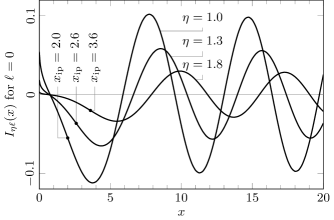
Figure 2: Plots of the regularized Coulomb wave function $\displaystyle I_{\eta\ell}(x)$ for the $\displaystyle s$ wave $\displaystyle(\ell=0)$ and different values of $\displaystyle\eta$. The inflection points $\displaystyle x_{\rm ip}$ are marked with a black dot. They lie at the same abscissa as for the usual Coulomb functions $\displaystyle F_{\eta\ell}(x)$ and $\displaystyle G_{\eta\ell}(x)$.

However, the functions $\displaystyle I^{\pm}_{\eta\ell}(x)$ and $\displaystyle I_{\eta\ell}(x)$ are not asymptotically normalized in the same way as the usual Coulomb functions, as shown in Fig. 2. Their wave amplitude is affected by $\displaystyle\eta$ and thus by the energy. The larger $\displaystyle\eta$, the wider the plateau below the inflection point, as with the regular Coulomb function $\displaystyle F_{\eta\ell}(x)$. It is interesting that $\displaystyle I_{\eta\ell}(x)$ combines some features of $\displaystyle G_{\eta\ell}(x)$ and $\displaystyle F_{\eta\ell}(x)$ near the origin. As shown in Fig. 2, $\displaystyle I_{\eta\ell}(x)$ shows the same singularity as $\displaystyle G_{\eta\ell}(x)$ at $\displaystyle x=0$.

The final analytic structure of $\displaystyle G_{\eta\ell}(x)$ can be obtained by averaging the decompositions of $\displaystyle H^{+}_{\eta\ell}(x)$ and $\displaystyle H^{-}_{\eta\ell}(x)$ from Eq. (40). One gets the analytic decomposition Yost et al. (1936); Breit et al. (1936); Cornille and Martin (1962); Abramowitz and Stegun (1964); Lambert (1969); Humblet (1984); Rakityansky and Elander (2013)

$$\boxed{G_{\eta\ell}(x)=\frac{\mathop{}\!\mathrm{e}^{2\eta\pi}-1}{\pi}\left[g_{\ell}(\eta)F_{\eta\ell}(x)+\frac{1}{w_{\eta\ell}}I_{\eta\ell}(x)\right]}\>,$$ (43)

where $\displaystyle I_{\eta\ell}(x)$ is the modified Coulomb function given by Eq. (42).

Our definition of $\displaystyle I_{\eta\ell}(x)$ has the advantage of being on a par with $\displaystyle F_{\eta\ell}(x)$ regarding the $\displaystyle k$-dependence. Indeed, Eqs. (26) and (39) show that both $\displaystyle F_{\eta\ell}/C_{\eta\ell}k^{\ell+1}$ and $\displaystyle I_{\eta\ell}/C_{\eta\ell}k^{\ell+1}$ are holomorphic in the $\displaystyle k$-plane and behave as a constant around the zero-energy point. This result has very important consequences in the framework of effective-range functions, as will be seen below. Moreover, Eq. (43) provides a clear identification of the singularities of the irregular Coulomb function $\displaystyle G_{\eta\ell}(x)$.

III Effective-range functions

The standard ERF is derived from the analysis of the Coulomb wave functions in the complex plane of the energy, when a short-range potential is added to the Coulomb potential. At the end of the section, the possible alternatives to the standard ERF are presented from the theoretical point of view.

III.1 Standard effective-range function

In this section, we show that the analytic decomposition (43) is responsible for the expression of the standard effective-range function. First, we assume that the potential $\displaystyle V(r)$ describing the interaction between the charged particles is modified by a short-range contribution of nuclear origin. Therefore, the wave function $\displaystyle u_{k\ell}(r)$ — that is equal to $\displaystyle F_{\eta\ell}(kr)$ for a pure Coulomb field — is altered in the nuclear region, whereas it merely acquires the phase shift $\displaystyle\delta_{\ell}(k)$ in the far-field region. The phase shift $\displaystyle\delta_{\ell}(k)$ is defined by the asymptotic behavior of the wave function $\displaystyle u_{k\ell}(r)$ up to a global normalization factor by Breit et al. (1936); Bethe (1949); Landau and Smorodinsky (1944); Blatt (1948); Chew and Goldberger (1949); Jackson and Blatt (1950); Messiah (1961); Gottfried (1966); Joachain (1979); Newton (1982); van Haeringen (1985); Humblet (1990)

$$u_{k\ell}(r)\xrightarrow{r\rightarrow\infty}F_{\eta\ell}(kr)\cos\delta_{\ell}(k)+G_{\eta\ell}(kr)\sin\delta_{\ell}(k)\>.$$ (44)

The phase shift follows from the continuity of the logarithmic derivative between the complete wave function $\displaystyle u_{k\ell}(r)$ and Eq. (44)

$$\frac{\partial_{r}u_{k\ell}(R)}{u_{k\ell}(R)}=\frac{\partial_{r}F_{\eta\ell}(kR)\cos\delta_{\ell}+\partial_{r}G_{\eta\ell}(kR)\sin\delta_{\ell}}{F_{\eta\ell}(kR)\cos\delta_{\ell}+G_{\eta\ell}(kR)\sin\delta_{\ell}}\>.$$ (45)

The matching point $\displaystyle r=R$ is chosen far enough for the phase shift to converge to an $\displaystyle R$-independent value. From Eq. (45), one gets the phase shift expressed as a ratio of Wronskians involving the complete wave function $\displaystyle u_{k\ell}(r)$ and the Coulomb functions

$$\cot\delta_{\ell}(k)=\frac{\operatorname{W}[G_{\eta\ell}(kr),u_{k\ell}(r)]_{R}}{\operatorname{W}[u_{k\ell}(r),F_{\eta\ell}(kr)]_{R}}\>,$$ (46)

where the notation of the Wronskian determinant is defined as

$$\operatorname{W}[f(x),g(x)]=f(x)\,\frac{\mathop{}\!\mathrm{d}g}{\mathop{}\!\mathrm{d}x}(x)-\frac{\mathop{}\!\mathrm{d}f}{\mathop{}\!\mathrm{d}x}(x)\,g(x)\>.$$ (47)

Using the analytic decomposition (43) of $\displaystyle G_{\eta\ell}(kr)$ the Wronskian in the numerator of Eq. (46) splits into two terms

$$\begin{split}\cot\delta_{\ell}(k)&=\frac{\mathop{}\!\mathrm{e}^{2\eta\pi}-1}{\pi}\\ &\times\left[\frac{1}{w_{\eta\ell}}\frac{\operatorname{W}[I_{\eta\ell}(kr),u_{k\ell}(r)]_{R}}{\operatorname{W}[u_{k\ell}(r),F_{\eta\ell}(kr)]_{R}}-g_{\ell}(\eta)\right]\>.\end{split}$$ (48)

The ratio of Wronskians in Eq. (48) involves $\displaystyle I_{\eta\ell}(kr)$ and $\displaystyle F_{\eta\ell}(kr)$, which both behave as $\displaystyle C_{\eta\ell}k^{\ell+1}$ in the neighborhood of $\displaystyle k=0$ as shown in Sec. II.2. Therefore, the ratio

$$\frac{\operatorname{W}[I_{\eta\ell}(kr),u_{k\ell}(r)]_{R}}{\operatorname{W}[u_{k\ell}(r),F_{\eta\ell}(kr)]_{R}}=w_{\eta\ell}\left[\frac{\pi\cot\delta_{\ell}(k)}{\mathop{}\!\mathrm{e}^{2\eta\pi}-1}+g_{\ell}(\eta)\right]$$ (49)

is analytic at zero energy and behaves as a constant near $\displaystyle k=0$, due to the cancellation of $\displaystyle C_{\eta\ell}k^{\ell+1}$ from $\displaystyle I_{\eta\ell}(kr)$ and $\displaystyle F_{\eta\ell}(kr)$. Indeed, all the possible poles of $\displaystyle u_{k\ell}(r)$ in the $\displaystyle k$-plane will simplify in the ratio. Consequently, one can define the Coulomb-modified effective-range function based on Eq. (49) Bethe (1949); Landau and Smorodinsky (1944); Blatt (1948); Chew and Goldberger (1949); Jackson and Blatt (1950); Cornille and Martin (1962); Lambert (1969); Joachain (1979); Newton (1982); Humblet (1990) as

$$\varkappa_{\ell}(k)=\frac{2w_{\eta\ell}}{\ell!^{2}a_{\mathrm{B}}^{2\ell+1}}\big{[}\Delta_{\ell}(k)+g_{\ell}(\eta)\big{]}\>,$$ (50)

where $\displaystyle\Delta_{\ell}(k)$ is the reduced effective-range function defined by

$$\Delta_{\ell}(k)=\frac{\pi\cot\delta_{\ell}(k)}{\mathop{}\!\mathrm{e}^{2\eta\pi}-1}\>,$$ (51)

that is discussed in further details in Sec. III.4. The function $\displaystyle\Delta_{\ell}(k)$ has been originally defined in Ref. Ramírez Suárez and Sparenberg (2017) with an additional factor $\displaystyle 2/a_{\mathrm{B}}$, but we omit it in this paper for convenience. The coefficient in Eq. (50) ensures that it reduces to the effective-range function of the neutral case

$$\varkappa_{\ell}(k)=k^{2\ell+1}\cot\delta_{\ell}(k)\>,$$ (52)

for vanishing charges ($\displaystyle a_{\mathrm{B}}^{-1}\rightarrow 0$) Bethe (1949); Landau and Smorodinsky (1944); Lambert (1969); Hamilton et al. (1973).

The function $\displaystyle\varkappa_{\ell}(k)$ in Eq. (50) being analytic at $\displaystyle E=0$, it has a useful series expansion in powers of the energy at this point Landau and Smorodinsky (1944); Bethe (1949); Blatt (1948); Chew and Goldberger (1949); Jackson and Blatt (1950); Lambert (1969); Hamilton et al. (1973); Joachain (1979); Kok (1980); Newton (1982); van Haeringen (1985), i.e., the effective-range expansion, which is usually written as

$$\varkappa_{\ell}(k)=-\frac{1}{\alpha_{\ell}}+\frac{r_{\ell}}{2}k^{2}+\operatorname{\mathcal{O}}(k^{4})\>,$$ (53)

where $\displaystyle\alpha_{\ell}$ is the scattering length and $\displaystyle r_{\ell}$ is the effective range. Higher-order terms in Eq. (53) also exist, see Naisse (1977); Kok (1980); Rakityansky and Elander (2013); Midya et al. (2015), but they are not discussed in this paper.

III.2 Properties of Bethe’s g function

Bethe’s function $\displaystyle g_{\ell}(\eta)$ is undoubtedly one of the most important functions of the effective-range theory of charged particles, as evidenced by its presence in Eq. (50).

Indeed, the analyticity of the traditional ERF $\displaystyle\varkappa_{\ell}(k)$ in Eq. (50) implies that any singular structure in $\displaystyle g_{\ell}(\eta)$ is reflected on the reduced ERF $\displaystyle\Delta_{\ell}(k)$ Ramírez Suárez and Sparenberg (2017). This is why it is so important to begin the study of $\displaystyle\Delta_{\ell}(k)$ with that of $\displaystyle g_{\ell}(\eta)$.

As a reminder, the function $\displaystyle g_{\ell}(\eta)$ is defined by Eqs. (32) and (41) as

$$g_{\ell}(\eta)=\frac{\psi(\ell+1+\mathrm{i}\eta)-\ln(\mathrm{i}\eta)+\psi(\ell+1-\mathrm{i}\eta)-\ln(-\mathrm{i}\eta)}{2}\>.$$ (54)

It is worth noting that Eq. (54) is not the usual function $\displaystyle g_{\ell}(\eta)$ that is defined in the literature, especially regarding the $\displaystyle\ell$-dependence. In Refs. Bethe (1949); Cornille and Martin (1962); Lambert (1969); Hamilton et al. (1973); Humblet (1990), it is often denoted as $\displaystyle h(\eta)$ or $\displaystyle g(\eta)$ and does not depend on $\displaystyle\ell$

$$g(\eta)=\frac{\psi(1+\mathrm{i}\eta)+\psi(1-\mathrm{i}\eta)}{2}-\ln\eta\>.$$ (55)

As will be seen below, the additional dependence on $\displaystyle\ell$ in Eq. (54) makes no difference in the ERF from the analytic point of view, except on the effective-range parameters of course.

Besides, the function $\displaystyle g_{\ell}(\eta)$ given by Eq. (54) reduces to Eq. (55) for the $\displaystyle s$ wave when $\displaystyle\ell=0$. Our formulation (54) has the advantage of being closer to the definition (24) of the function $\displaystyle G_{\eta\ell}(kr)$ from which $\displaystyle g_{\ell}(\eta)$ originates.

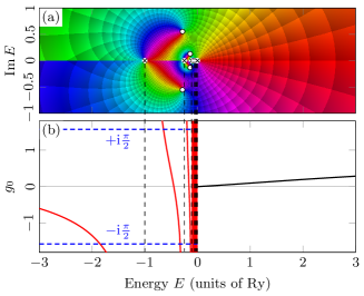
Figure 3: (Color online) Representations of the principal branch of $\displaystyle g_{\ell}(\eta)$ for $\displaystyle\ell=0$ (a) in the complex plane of the energy $\displaystyle E$ and (b) along the real $\displaystyle E$-axis. In (a), the conventional branch cut lies along the negative real $\displaystyle E$-axis. Throughout this paper, real functions are depicted in solid black. Where functions are complex, the real part is shown in solid red (dark gray) and the imaginary part in dashed blue. In (b), the imaginary part is either $\displaystyle+\mathrm{i}\pi/2$ (if $\displaystyle\arg E=+\pi$) or $\displaystyle-\mathrm{i}\pi/2$ (if $\displaystyle\arg E=-\pi$).

The function $\displaystyle g_{\ell}(\eta)$ is shown in Fig. 3 for $\displaystyle\ell=0$. It is a real function at positive energy but complex valued everywhere else, especially on the negative real $\displaystyle E$-axis.

One of the most noticeable structures is the array of poles at negative energies due to the digamma functions $\displaystyle\psi(\ell+1\pm\mathrm{i}\eta)$. In the energy plane, they are located at

$$k_{{\rm C},n}=\frac{\pm\mathrm{i}}{(n+\ell+1)a_{\mathrm{B}}}\quad\text{and}\quad E_{{\rm C},n}=\frac{\hbar^{2}}{2m}k_{{\rm C},n}^{2}\>,$$ (56)

for $\displaystyle n\in\{0,1,\ldots\}$, so that $\displaystyle E=0$ is an accumulation point of poles and thus an essential singularity of $\displaystyle g_{\ell}(\eta)$. Remarkably, the poles of Eq. (56) lie at the same energies as the hydrogen-like levels due to the $\displaystyle\ell$-dependence of $\displaystyle g_{\ell}(\eta)$. These poles are not related to bound states since the corresponding poles of the reduced ERF $\displaystyle\Delta_{\ell}(k)$ have no such interpretation.

In addition to the poles, the function $\displaystyle g_{\ell}(\eta)$ also shows infinitely many zeroes near the poles accumulating at $\displaystyle E=0$, as shown in Fig. 3(a). The pole-zero screening explains why the function becomes suddenly smooth at positive energy.

Such a smoothness of $\displaystyle g_{\ell}(\eta)$ at positive energy may suggest that it is analytic at $\displaystyle E=0$ and can be expanded in series at this point. If such an expansion was found, the function $\displaystyle g_{\ell}(\eta)$ could be merely omitted from the Coulomb-modified ERF (50) as proposed in Ramírez Suárez and Sparenberg (2017), since $\displaystyle\Delta_{\ell}(k)$ would also be analytic. However, because of the essential singularity at $\displaystyle E=0$, the function $\displaystyle g_{\ell}(\eta)$ is not analytic at this point, meaning that no Taylor expansion is expected to converge in a finite neighborhood of $\displaystyle E=0$.

On the other hand, according to Refs. Olver et al. (2010); Abramowitz and Stegun (1964), the digamma function $\displaystyle\psi(z)$ has an asymptotic Stirling expansion at $\displaystyle\left|z\right|\rightarrow\infty$ in all directions except the poles $\displaystyle\left|\arg z\right|<\pi-\varepsilon$ ($\displaystyle\varepsilon>0$). The corresponding asymptotic low-energy behavior of $\displaystyle g_{\ell}(\eta)$ reads

$$g_{\ell}(\eta)\sim-\sum_{n=1}^{\infty}\frac{B_{2n}}{2n}(\mathrm{i}a_{\mathrm{B}}k)^{2n}+\sum_{s=0}^{\ell}\frac{(a_{\mathrm{B}}k)^{2}s}{1+(a_{\mathrm{B}}ks)^{2}}\>,$$ (57)

for $\displaystyle\left|E\right|\ll 1~{}\mathrm{Ry}$ and $\displaystyle\left|\arg E\right|<\pi-\varepsilon$. The coefficients $\displaystyle B_{2n}$ in Eq. (57) are the Bernoulli numbers. They are known to dramatically increase with $\displaystyle n$ Olver et al. (2010); Abramowitz and Stegun (1964)

$$\frac{B_{2n}}{2n}\sim(-1)^{n+1}\frac{2\,\Gamma(2n)}{(2\pi)^{2n}}\quad\text{for}~{}n\rightarrow\infty\>.$$ (58)

Such an increase reduces to zero the radius of convergence of (57).

Regarding the other kinds of rational expansion, the logarithmic branch cut seen in Fig. 3(a) along the negative real $\displaystyle E$-axis will prevent the approximants from converging to $\displaystyle g_{\ell}(\eta)$. The logarithmic component in $\displaystyle g_{\ell}(\eta)$ is also evidenced by its high-energy behavior

$$g_{\ell}(\eta)=\psi(\ell+1)-\ln(\eta)+\operatorname{\mathcal{O}}(\eta)\>,$$ (59)

for $\displaystyle\left|E\right|\gg 1~{}\mathrm{Ry}$. The behavior (59) also means that $\displaystyle g_{\ell}(\eta)$ is a flat function at significantly higher energies than the nuclear Rydberg.

Besides the function $\displaystyle g_{\ell}(\eta)$, there are other important functions defined in the literature (see Cornille and Martin (1962); Hamilton et al. (1973); van Haeringen (1985); Kok (1980); Humblet (1984)): namely the functions $\displaystyle h^{\pm}_{\ell}(\eta)$. As for $\displaystyle g_{\ell}(\eta)$, they are typically encountered in their $\displaystyle\ell$-independent version. We define it with a dependence in $\displaystyle\ell$

$$h^{\pm}_{\ell}(\eta)=\psi(\pm\mathrm{i}\eta)+\frac{1}{\pm 2\mathrm{i}\eta}-\ln(\pm\mathrm{i}\eta)+\sum_{s=0}^{\ell}\frac{s}{s^{2}+\eta^{2}}\>,$$ (60)

so that they are on an equal footing with $\displaystyle g_{\ell}(\eta)$. This function is discussed further in Sec. III.3.

The important properties of $\displaystyle h^{\pm}_{\ell}(\eta)$ are Cornille and Martin (1962); Hamilton et al. (1973)

$$\begin{cases}\frac{h^{+}_{\ell}(\eta)+h^{-}_{\ell}(\eta)}{2}=g_{\ell}(\eta)\>,\\[5.0pt] \frac{h^{+}_{\ell}(\eta)-h^{-}_{\ell}(\eta)}{2\mathrm{i}}=\frac{\pi}{\mathop{}\!\mathrm{e}^{2\eta\pi}-1}\>.\end{cases}$$ (61)

In other words, $\displaystyle g_{\ell}(\eta)$ can be looked upon as the real part of either $\displaystyle h^{+}_{\ell}(\eta)$ or $\displaystyle h^{-}_{\ell}(\eta)$ at positive energy, since they are complex conjugated to each other Hamming (1973). In addition, the imaginary part of $\displaystyle h^{+}_{\ell}(\eta)$ at $\displaystyle E>0$ is nothing but the Coulomb factor $\displaystyle\pi/(\mathop{}\!\mathrm{e}^{2\eta\pi}-1)$, as it appears in Eq. (43).

Finally, it is possible to express the far-field behavior of $\displaystyle I_{\eta\ell}(kr)$ substituting the asymptotic formulae of $\displaystyle F_{\eta\ell}(x)$ and $\displaystyle G_{\eta\ell}(x)$ into Eq. (43) and using the properties (61) to get for positive energies

$$\begin{split}I_{\eta\ell}(x)&\xrightarrow{x\rightarrow\infty}-w_{\eta\ell}\left|h^{+}_{\ell}(\eta)\right|\\ \times&\sin\left(x-\ell\frac{\pi}{2}-\eta\ln(2x)+\sigma_{\eta\ell}-\arg h^{+}_{\ell}(\eta)\right)\>.\end{split}$$ (62)

III.3 Effective-range function by Hamilton et al.

Before studying further the function $\displaystyle\Delta_{\ell}(k)$, it is useful to take a look at other functions envisioned as potential alternatives to the traditional ERF $\displaystyle\varkappa_{\ell}(k)$. One of the drawbacks of $\displaystyle\Delta_{\ell}(k)$ is the presence of expected Coulomb poles at negative energy predicted by the analysis of $\displaystyle g_{\ell}(\eta)$ in Sec. III.2. These poles symmetrically occur in both the physical ($\displaystyle\operatorname{Im}k>0$) and the unphysical sheet ($\displaystyle\operatorname{Im}k<0$), possibly impairing the study of negative energies with $\displaystyle\Delta_{\ell}(k)$.

However, there is a way to partially overcome the issue by removing the poles of $\displaystyle g_{\ell}(\eta)$ from the physical sheet. One idea is to apply the reflection formula of the digamma function Abramowitz and Stegun (1964); Olver et al. (2010) to $\displaystyle\psi(\ell+1-\mathrm{i}\eta)$ in Eq. (54), which is responsible for the poles on the positive imaginary $\displaystyle k$-axis. For this purpose, we use the property

$$\psi(\ell+1-\mathrm{i}\eta)=\psi(\mathrm{i}\eta)-\mathrm{i}\pi-\frac{2\mathrm{i}\pi}{\mathop{}\!\mathrm{e}^{2\eta\pi}-1}+\sum_{s=1}^{\ell}\frac{1}{s-\mathrm{i}\eta}\>,$$ (63)

where the remaining digamma function $\displaystyle\psi(\mathrm{i}\eta)$ only has poles in the unphysical sheet. Inserting Eq. (63) into the expression (54) of $\displaystyle g_{\ell}(\eta)$ provides the relation

$$g_{\ell}(\eta)=h^{+}_{\ell}(\eta)-\frac{\mathrm{i}\pi}{\mathop{}\!\mathrm{e}^{2\eta\pi}-1}\>,$$ (64)

where one notices the appearance of the function $\displaystyle h^{+}_{\ell}(\eta)$ defined in Eq. (60). Indeed, the relation (64) directly follows from Eq. (61).

Furthermore, the decomposition (64) leads to new formulation of the usual ERF $\displaystyle\varkappa_{\ell}(k)$ due to Cornille and Martin Cornille and Martin (1962) and Hamilton et al. Hamilton et al. (1973)

$$\varkappa_{\ell}(k)=\frac{2w_{\eta\ell}}{\ell!^{2}a_{\mathrm{B}}^{2\ell+1}}\bigg{[}\underbrace{\frac{\pi[\cot\delta_{\ell}(k)-\mathrm{i}]}{\mathop{}\!\mathrm{e}^{2\eta\pi}-1}}_{\Delta^{+}_{\ell}(k)}+h^{+}_{\ell}(\eta)\bigg{]}\>,$$ (65)

where $\displaystyle\Delta^{+}_{\ell}(k)$ embeds the remaining exponential term in Eq. (64) Hamilton et al. (1973). The calculation being symmetric for $\displaystyle h^{+}_{\ell}(\eta)$ and $\displaystyle h^{-}_{\ell}(\eta)$, one defines the two notations accordingly

$$\Delta^{\pm}_{\ell}(k)=\Delta_{\ell}(k)\mp\frac{\mathrm{i}\pi}{\mathop{}\!\mathrm{e}^{2\eta\pi}-1}=\frac{\pi[\cot\delta_{\ell}(k)\mp\mathrm{i}]}{\mathop{}\!\mathrm{e}^{2\eta\pi}-1}\>.$$ (66)

The function $\displaystyle\Delta^{+}_{\ell}(k)$ is denoted as $\displaystyle F_{0}^{-1}$ in Hamilton et al. (1973) up to the factor $\displaystyle 2/a_{\mathrm{B}}$, and has been applied more recently to the ${}^{2}\mathrm{H}+\alpha$ elastic scattering process by Blokhintsev et al. Blokhintsev et al. (2017a, b).

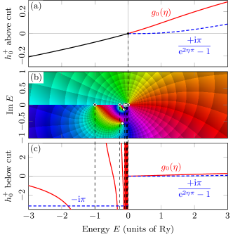
Figure 4: (Color online) Plots of the principal branch of $\displaystyle h^{+}_{\ell}(\eta)$ for $\displaystyle\ell=0$ (b) in the complex $\displaystyle E$-plane, (a) along the real $\displaystyle E$-axis in the physical sheet ($\displaystyle\arg E=0,+\pi$) and (c) along the real axis in the unphysical sheet ($\displaystyle\arg E=0,-\pi$). The function is complex valued for $\displaystyle\arg E=0$ but real for $\displaystyle\arg E=+\pi$. In (c), $\displaystyle h^{+}_{0}(\eta)$ is complex valued and shows the Coulomb poles.

Similarly to $\displaystyle g_{\ell}(\eta)$ and $\displaystyle\Delta_{\ell}(k)$, the function $\displaystyle h^{+}_{\ell}(\eta)$ is indicative of the behavior of $\displaystyle\Delta^{+}_{\ell}(k)$ in the $\displaystyle k$-plane. As shown in Fig. 4, $\displaystyle h^{+}_{\ell}(\eta)$ — and thus $\displaystyle\Delta^{+}_{\ell}(k)$ — is complex valued at positive energy, but real on the positive imaginary $\displaystyle k$-axis, that is to say at negative energy above the branch cut ($\displaystyle\arg E=+\pi$). This property is due to the compensation between the constant imaginary part $\displaystyle-\mathrm{i}\pi/2$ of $\displaystyle\mathrm{i}\pi/(\mathop{}\!\mathrm{e}^{2\eta\pi}-1)$ and the imaginary part $\displaystyle+\mathrm{i}\pi/2$ of $\displaystyle g_{\ell}(\eta)$ at $\displaystyle\arg E=+\pi$, as shown in Fig. 3(b). Below the branch cut ($\displaystyle\arg E=-\pi$), the function $\displaystyle h^{+}_{\ell}(\eta)$ is complex valued and has the same Coulomb poles as $\displaystyle g_{\ell}(\eta)$, but not the same zeroes. Therefore, although it is smooth near $\displaystyle E=0$ in Fig. 4(a), the function $\displaystyle\Delta^{+}_{\ell}(k)$ is still not analytic at $\displaystyle E=0$. In this respect, the use of $\displaystyle\Delta^{+}_{\ell}(k)$ as a potential substitute for the traditional ERF $\displaystyle\varkappa_{\ell}(k)$ is very debatable. This topic has never been pursued in the literature until now Blokhintsev et al. (2017a, b); Ramírez Suárez and Sparenberg (2017).

It should be noted that $\displaystyle\Delta^{+}_{\ell}(k)$ has the great advantage of mimicking the denominator of the Coulomb-modified scattering matrix element Gottfried (1966); Joachain (1979); Newton (1982)

$$S_{\ell}(k)=\mathop{}\!\mathrm{e}^{2\mathrm{i}\sigma_{\eta\ell}}\,\frac{\cot\delta_{\ell}(k)+\mathrm{i}}{\cot\delta_{\ell}(k)-\mathrm{i}}=\mathop{}\!\mathrm{e}^{2\mathrm{i}\sigma_{\eta\ell}}\,\frac{\Delta^{-}_{\ell}(k)}{\Delta^{+}_{\ell}(k)}\>.$$ (67)

Therefore, the poles of $\displaystyle S_{\ell}(k)$ are merely given by the zeroes of $\displaystyle\Delta^{+}_{\ell}(k)$ Blokhintsev et al. (2017a).

Using a two-term approximation of the effective-range expansion given by Eq. (53) and the ERF of Eq. (65), the equation of bound and resonant states $\displaystyle\Delta^{+}_{\ell}(k)=0$ can also be written as

$$w_{\eta\ell}\,h^{+}_{\ell}(\eta)=\frac{\ell!^{2}a_{\mathrm{B}}^{2\ell+1}}{2}\left(-\frac{1}{\alpha_{\ell}}+\frac{r_{\ell}}{2}k^{2}\right)\>,$$ (68)

to be solved for the unknowns $\displaystyle k$ and $\displaystyle\eta$ using Eq. (4).

When searching for bound states numerically, it is more appropriate to solve Eq. (68) in the $\displaystyle k$-plane than in the $\displaystyle E$-plane. As shown in Fig. 4(b), the branch cut of the principal-valued function $\displaystyle h^{+}_{\ell}(\eta)$ along the negative $\displaystyle E$-axis will prevent most iterative root-finding methods from converging to the bound state. The practical advantage of the $\displaystyle k$-representation of $\displaystyle h^{+}_{\ell}(\eta)$ is the absence of any singularity in the physical sheet.

If, in addition, we consider the $\displaystyle s$ wave at energies low enough that the effective-range term $\displaystyle r_{0}k^{2}/2$ is negligible, the equation (68) for bound and resonant states takes the form

$$h^{+}_{0}(\eta)=\psi(\mathrm{i}\eta)+\frac{1}{2\mathrm{i}\eta}-\ln(\mathrm{i}\eta)=\frac{-a_{\mathrm{B}}}{2\alpha_{0}}\>.$$ (69)

This equation is encountered with Dirac delta-plus-Coulomb potentials, since the effective-range $\displaystyle r_{0}$ is zero as well as any higher order coefficient Albeverio et al. (1988).

The solutions of Eq. (69) can be found graphically in Fig. 4(a) based on the scattering length $\displaystyle\alpha_{0}$. When $\displaystyle\alpha_{0}$ is positive then the solution can be interpreted as a bound state because $\displaystyle h^{+}_{0}(\eta)$ can match $\displaystyle-a_{\mathrm{B}}/2\alpha_{0}$ at negative energy. Otherwise, if $\displaystyle\alpha_{0}<0$, the solution is interpreted as a resonance. In the latter case, the zero of $\displaystyle\Delta^{+}_{\ell}(k)$ deviates from the real $\displaystyle E$-axis towards the unphysical sheet so as to follow the level curve defined by $\displaystyle\operatorname{Im}h^{+}_{\ell}(\eta)=0$ in Fig. 4(b). This curve is referred to as “universal” in Ref. Kok (1980), although it is only valid at zeroth-order approximation of the effective-range theory, as in Eq. (69).

III.4 Reduced effective-range function

We are now focusing on the properties of the reduced ERF $\displaystyle\Delta_{\ell}(k)$ and its potential interest in low-energy scattering. As recently highlighted in Ramírez Suárez and Sparenberg (2017), a major drawback of the usual ERF $\displaystyle\varkappa_{\ell}(k)$ is the overwhelming dominance of $\displaystyle g_{\ell}(\eta)$ upon the phase-shift-dependent part $\displaystyle\Delta_{\ell}(k)$, which occurs especially with heavy and moderately heavy nuclei. This imbalance comes from the smallness of the exponential prefactor $\displaystyle\pi/(\mathop{}\!\mathrm{e}^{2\eta\pi}-1)$ at typical energies encountered in low-energy nuclear scattering experiments ($\displaystyle<10~{}\mathrm{Ry}$)

$$\frac{\pi}{\mathop{}\!\mathrm{e}^{2\eta\pi}-1}\ll g_{0}(\eta)\quad\text{for}~{}\eta\gtrsim 1\>.$$ (70)

For instance, at $\displaystyle E=0.1~{}\mathrm{Ry}$, the Sommerfeld parameter is $\displaystyle\eta=\sqrt{10}$ and the factor $\displaystyle\pi/(\mathop{}\!\mathrm{e}^{2\eta\pi}-1)$ is about $\displaystyle 10^{6}$ times smaller than the function $\displaystyle g_{0}(\eta)$. The greatness of $\displaystyle g_{\ell}(\eta)$ is a potential problem while interpolating $\displaystyle\varkappa_{\ell}(k)$ because it may conceal the structures in $\displaystyle\Delta_{\ell}(k)$ due to the phase shift. Therefore, the addition of $\displaystyle g_{\ell}(\eta)$ could lead to an underfitting of the phase-shift-dependent part $\displaystyle\Delta_{\ell}(k)$ of the usual ERF, as done in Refs. Orlov et al. (2016, 2017).

One easy way to avoid this drawback is to directly approach the experiment-based function $\displaystyle\Delta_{\ell}(k)$ by an expansion of the form

$$\Delta_{\ell}(k)=-g_{\ell}(\eta)+\frac{\ell!^{2}a_{\mathrm{B}}^{2\ell+1}}{2w_{\eta\ell}}\left[\frac{-1}{\alpha_{\ell}}+\frac{r_{\ell}}{2}k^{2}+\operatorname{\mathcal{O}}(k^{4})\right]\>.$$ (71)

It has the advantage of being perfectly consistent with the usual effective-range method (50). But now, there is no more risk of superposition between large and small quantities.

The peculiar properties of the functions $\displaystyle h^{\pm}_{\ell}(\eta)$ and $\displaystyle g_{\ell}(\eta)$ allow us to go a little further. As shown in Eq. (64), the only difference between $\displaystyle h^{+}_{\ell}(\eta)$ and $\displaystyle g_{\ell}(\eta)$ is the exponential term behaving like

$$\frac{\mathrm{i}\pi}{\mathop{}\!\mathrm{e}^{2\eta\pi}-1}\sim\mathrm{i}\pi\mathop{}\!\mathrm{e}^{-2\pi/a_{\mathrm{B}}k}\quad\text{as}~{}E\xrightarrow{>}0\>.$$ (72)

Accordingly, the asymptotic expansion of $\displaystyle\mathrm{i}\pi/(\mathop{}\!\mathrm{e}^{2\eta\pi}-1)$ is zero at $\displaystyle E=0$ (for $\displaystyle E>0$) due to the essential singularity at this point. Therefore, the function $\displaystyle h^{+}_{\ell}(\eta)$ has the same asymptotic expansion (57) as $\displaystyle g_{\ell}(\eta)$

$$h^{+}_{\ell}(\eta)\sim-\sum_{n=1}^{n_{\max}}\frac{B_{2n}}{2n}(\mathrm{i}a_{\mathrm{B}}k)^{2n}+\sum_{s=0}^{\ell}\frac{(a_{\mathrm{B}}k)^{2}s}{1+(a_{\mathrm{B}}ks)^{2}}\>,$$ (73)

for $\displaystyle E\rightarrow 0$ but in the physical sheet ($\displaystyle\operatorname{Im}k\geq 0$) as the order $\displaystyle n_{\max}$ tends to infinity. This shows that $\displaystyle h^{+}_{\ell}(\eta)$ and $\displaystyle g_{\ell}(\eta)$ come together smoothly at the origin in the physical sheet, as evidenced by Fig. 4(a). Since the two functions $\displaystyle h^{+}_{\ell}(\eta)$ and $\displaystyle g_{\ell}(\eta)$ are similar to $\displaystyle\Delta^{+}_{\ell}(k)$ and $\displaystyle\Delta_{\ell}(k)$ respectively, the above statement also means that $\displaystyle\Delta^{+}_{\ell}(k)$ and $\displaystyle\Delta_{\ell}(k)$ smoothly join at $\displaystyle E=0$ in the physical sheet.

To some extent, this property can be exploited to extrapolate low-energy data to negative energies using $\displaystyle\Delta_{\ell}(k)$ instead of the traditional ERF, as done in Refs. Ramírez Suárez and Sparenberg (2017); Blokhintsev et al. (2017a, b). Indeed, it is possible that the direct interpolation $\displaystyle\Delta_{\ell}^{\mathrm{fit}}(k)$ of the experiment-based function $\displaystyle\Delta_{\ell}(k)$ locally provides a reasonable estimate of $\displaystyle\Delta^{+}_{\ell}(k)$ at negative energies in the physical sheet

$$\Delta_{\ell}^{\mathrm{fit}}(k)\sim\begin{cases}\Delta_{\ell}(k)&\textrm{for}~{}\arg E=0\>,\\[5.0pt] \Delta^{+}_{\ell}(k)&\textrm{for}~{}\arg E=+\pi\>.\end{cases}$$ (74)

Therefore, the negative-energy zeroes of $\displaystyle\Delta_{\ell}^{\mathrm{fit}}(k)$ can be interpreted as bound states, as long as they are located in a region of low energy (typically $\displaystyle\left|E\right|\ll 1~{}\mathrm{Ry}$).

However, it should be noted that such a method is not guaranteed to provide reliable results, because $\displaystyle\Delta_{\ell}(k)$ and $\displaystyle\Delta^{+}_{\ell}(k)$ are not analytic at $\displaystyle E=0$. The smoothness of $\displaystyle\Delta^{+}_{\ell}(k)$ at $\displaystyle E=0$ in the physical sheet is not enough to consider it as analytic, because of the essential singularity at $\displaystyle E=0$ [see the accumulation of poles in Fig. 4(c)]. Attempting to interpolate $\displaystyle\Delta_{\ell}(k)$ by a meromorphic function like a Padé approximant is likely to lead to undetermined behaviors, without possible convergence to $\displaystyle\Delta^{+}_{\ell}(k)$.

In addition, the analytic continuation of the function $\displaystyle\Delta_{\ell}(k)$ is multi-valued due to its logarithmic component discussed in Sec. III.2. Such a feature cannot be interpolated by a Padé approximant. If, though, it is done, the fitted Padé approximant would attempt to accumulate spurious poles on the negative $\displaystyle E$-axis to come closer to the branch cut. This will be discussed further in Sec. IV.

On the other hand, it is possible to quantify the accuracy of the asymptotic expansion (73). This should help to estimate the minimum error made when approaching $\displaystyle\Delta_{\ell}(k)$ with a polynomial in $\displaystyle E$. Indeed, despite the convergence of $\displaystyle\Delta_{\ell}^{\mathrm{fit}}(k)$ is not expected as the order increases, it may provide useful interpolation in a low enough energy range.

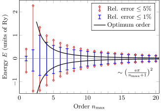
Figure 5: Energy intervals where the relative error of the truncated Stirling expansion (73) of $\displaystyle h^{+}_{\ell}(\eta)$ (for $\displaystyle\ell=0$) does not exceed $\displaystyle 5\%$ and $\displaystyle 1\%$. The expected optimum order $\displaystyle n_{\rm opt}$ of Eq. (76) is shown in solid black.

For this purpose, we compute the energy intervals where the relative error in the truncated Stirling series (73) does not exceed $\displaystyle 1\%$ to $\displaystyle 5\%$ as a function of the order $\displaystyle n_{\max}$. The result is shown in Fig. 5.

The expansion obviously diverges since the region of validity, represented by vertical bars, continues to decrease. At high orders, an approximate calculation involving Eq. (58) shows that the energy interval roughly decreases like $\displaystyle[\mathop{}\!\mathrm{e}\pi/(n_{\max}+1)]^{2}~{}\mathrm{Ry}$ as $\displaystyle n_{\max}\rightarrow\infty$, independently of the bound on the relative error.

Beyond about $\displaystyle 1~{}\mathrm{Ry}$, the error is larger than $\displaystyle 5\%$ whatever the order $\displaystyle n_{\max}$ in Eq. (73). This suggests that, as long as no data point is known in the interval $\displaystyle[-1,1]~{}\mathrm{Ry}$, the interpolation of $\displaystyle\Delta_{\ell}(k)$ will not be of practical interest at $\displaystyle E<0$.

However, it is possible to get relatively accurate results if data points are known at energies below $\displaystyle 1~{}\mathrm{Ry}$. This case is typically encountered for heavy and moderately heavy particles. In addition, the intervals in Fig. 5 allow us to roughly estimate the maximum order $\displaystyle n_{\max}$ before a polynomial interpolation of $\displaystyle\Delta_{\ell}(k)$ will stray too much from $\displaystyle\Delta^{+}_{\ell}(k)$ depending on the energy range considered.

Moreover, there is an optimum order that minimizes the error of the asymptotic series in Eq. (73). It also corresponds to the smallest term of this series. To get it for the $\displaystyle s$ wave, one cancels the logarithmic derivative of the $\displaystyle n$th term in Eq. (73) using the asymptotic behavior (58)

$$\frac{\mathop{}\!\mathrm{d}}{\mathop{}\!\mathrm{d}n}\big{[}\ln\Gamma(2n)-2n\ln\left|2\eta\pi\right|\big{]}=0\>.$$ (75)

This is a suitable approximation provided that the sought index $\displaystyle n$ is larger than $\displaystyle 1$. The approximate solution of Eq. (75), rounded to the closest integer, is

$$n_{\rm opt}\simeq\pi\left|\eta\right|=\pi\sqrt{\frac{\mathrm{Ry}}{\left|E\right|}}\>.$$ (76)

The curve of the optimum order $\displaystyle n_{\rm opt}$ is shown in Fig. 5. Above $\displaystyle n_{\rm opt}$, the Stirling series in Eq. (73) starts diverging.

IV Application to proton-proton collision

In this section, we propose to apply the effective-range theory to the ${}^{1}S_{0}$ elastic scattering of two protons. Indeed, this two-body system is of historical importance and is greatly documented in the literature, especially in Refs. Breit et al. (1936); Landau and Smorodinsky (1944); Blatt (1948); Bethe (1949); Chew and Goldberger (1949); Jackson and Blatt (1950); Naisse (1977); Kok (1980); Bergervoet et al. (1988); Mukhamedzhanov et al. (2010). This section is divided into two parts: the first one is about the graphical representation of the previously discussed effective-range functions $\displaystyle\Delta_{\ell}(k)$, $\displaystyle\Delta^{+}_{\ell}(k)$ and $\displaystyle\varkappa_{\ell}(k)$ at real and complex energies, and the second one is about the practical use of the reduced ERF $\displaystyle\Delta_{\ell}(k)$ Ramírez Suárez and Sparenberg (2017) in the framework of proton-proton collision. As a reminder, the orders of magnitude for the proton-proton system are mainly governed by the nuclear Rydberg energy: $\displaystyle 1~{}\mathrm{Ry}=12.49~{}\mathrm{keV}$ Bethe (1949).

IV.1 Effective-range functions in the $\displaystyle\boldsymbol{E}$-plane

In order to reproduce the phase shift $\displaystyle\delta_{\ell}(k)$ and the related quantities for the proton-proton scattering, we resort to the square-well model. We assume the total potential $\displaystyle V(r)$ to be constant in the short-range region $\displaystyle r\leq R$

$$V(r)=\begin{cases}V_{0}&\text{if}~{}r\leq R\>,\\[3.0pt] \frac{\alpha\hbar c}{r}&\text{if}~{}r>R\>,\end{cases}$$ (77)

with typically negative $\displaystyle V_{0}$. This simple model should be sufficient to describe the functions of interest at relatively low energy, i.e., below about $\displaystyle 5~{}\mathrm{MeV}$ for proton-proton.

Such an approach is similar to what has recently been done by Blokhintsev et al. in Blokhintsev et al. (2017a). However, we assume the additional potential compensates for Coulomb interaction in the nuclear region $\displaystyle r\leq R$. This provides a total potential $\displaystyle V(r)$ that is both simple and practical. This choice has no consequences at low energy, but it modifies the high-energy limit of the effective-range functions.

The square-well model has the advantage of being exactly solvable. This will be quite useful in the following to perform the analytic continuation of the functions to the complex $\displaystyle E$-plane. In the short-range region, the wave function $\displaystyle u_{k\ell}(r)$ is described by the spherical Bessel functions $\displaystyle j_{\ell}(z)$ Messiah (1961); Gottfried (1966); Joachain (1979); Newton (1982)

$$u_{k\ell}(r)=qr\,j_{\ell}(qr)\quad\text{for}~{}r\leq R\>,$$ (78)

where $\displaystyle q$ is the local wave number given by

$$q=\sqrt{k^{2}-\frac{2m}{\hbar^{2}}V_{0}}\>.$$ (79)

Then, we compute $\displaystyle\cot\delta_{\ell}(k)$ from Eq. (46) using the recurrence properties of the Coulomb wave functions to compute their derivatives Olver et al. (2010). The computation is done in the Wolfram Mathematica software Wolfram (1999) using the implementation of the confluent hypergeometric functions $\displaystyle M(a,b,z)$ and $\displaystyle U(a,b,z)$ defined for complex arguments.

Finally, the parameters $\displaystyle R$ and $\displaystyle V_{0}$ of the potential well are fitted to reproduce the effective-range parameters $\displaystyle\alpha_{0}$ and $\displaystyle r_{0}$ for the proton-proton ${}^{1}S_{0}$ channel as given by Refs. Naisse (1977); Bergervoet et al. (1988)

$$\begin{cases}\alpha_{0}=-7.81~{}\mathrm{fm}\>,\\ r_{0}=2.79~{}\mathrm{fm}\>.\end{cases}$$ (80)

We obtain the parameters

$$\begin{cases}R=2.8~{}\mathrm{fm}\>,\\ V_{0}=-10.66~{}\mathrm{MeV}\>.\end{cases}$$ (81)

In the following subsections, all the phase-shift-related quantities have been computed for the square-well model with the parameters of Eq. (81).

IV.1.1 Proton-proton reduced effective-range function

The reduced ERF $\displaystyle\Delta_{0}(E)$ of the proton-proton $\displaystyle s$ wave is represented in the complex plane of the energy in Figs. 6 and 7.

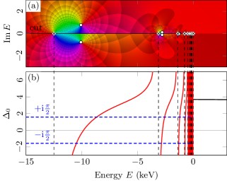
Figure 6: (Color online) Function $\displaystyle\Delta_{0}(E)$ for the proton-proton ${}^{1}S_{0}$ scattering (a) in the complex $\displaystyle E$-plane and (b) on the real $\displaystyle E$-axis. The function is real and positive at $\displaystyle E>0$ but complex-valued at $\displaystyle E<0$. In (a), the branch cut along the negative $\displaystyle E$-axis is depicted by a black line. The imaginary part around the cut is either $\displaystyle-\mathrm{i}\pi/2$ (if $\displaystyle\arg E=+\pi$) or $\displaystyle+\mathrm{i}\pi/2$ (if $\displaystyle\arg E=-\pi$).

Figure 7: (Color online) Same as Fig. 6 but at higher energies. At this scale, the Coulomb poles look merged at $\displaystyle E=0$. The two zeroes are located at about $\displaystyle E=(-1.75\pm 1.33\,\mathrm{i})~{}\mathrm{MeV}$.

The function $\displaystyle\Delta_{0}(E)$ is shown at two different scales because of the large disparity of the orders of magnitude for this system. Indeed, $\displaystyle\Delta_{0}(E)$ is almost linear beyond roughly $\displaystyle 2~{}\mathrm{MeV}$ in Fig. 7(b), but also has poles below $\displaystyle 1~{}\mathrm{Ry}=12.49~{}\mathrm{keV}$ accumulating at $\displaystyle E=0$ on the negative real $\displaystyle E$-axis in Fig. 6.

It should be noted that these poles exactly correspond to the Coulomb poles of $\displaystyle g_{0}(\eta)$ given by Eq. (56). The Coulombic nature of the poles of $\displaystyle\Delta_{0}(E)$ can be checked by observing that they are independent of the nuclear potential depth $\displaystyle V_{0}$. Besides, the function $\displaystyle\Delta_{0}(E)$ also shows an accumulation of zeroes at $\displaystyle E=0$ that are compensating for the poles, hence the smooth behavior at $\displaystyle E>0$. The two high-energy zeroes of $\displaystyle\Delta_{0}(E)$ in Fig. 7(a) are located at about $\displaystyle E=(-1.75\pm 1.33\,\mathrm{i})~{}\mathrm{MeV}$, and correspond to points where the scattering matrix from Eq. (67) amounts to $\displaystyle-1$ up to a pure Coulomb phase. Unlike the Coulomb poles, all these zeroes depend on the parameters of the nuclear potential.

In addition, $\displaystyle\Delta_{0}(E)$ possesses a branch cut clearly visible in Fig. 7(a) and highlighted by a black line in Fig. 6(a). The cut stops at $\displaystyle E=0$ and the function is smooth at positive energy.

Furthermore, the function $\displaystyle\Delta_{0}(E)$ shows two very different structures for positive and negative real energies in Fig. 6(b) due to the essential singularity at this point. This could suggest that $\displaystyle\Delta_{0}(E)$ is piecewise defined. However, Fig. 6(a) shows that there is no such thing, because these two pieces belong to the same Riemann surface through analytic continuation.

Finally, all these low-energy structures confirm that $\displaystyle\Delta_{0}(E)$ behaves as predicted by the expansion (71) of the effective-range theory.

IV.1.2 Proton-proton effective-range function by Hamilton et al.

The ERF $\displaystyle\Delta^{+}_{0}(E)$ by Hamilton et al. Hamilton et al. (1973) for the two-proton system is shown in Fig. 8 at relatively high energies with respect to the nuclear Rydberg energy of $\displaystyle 12.49~{}\mathrm{keV}$. The plot of $\displaystyle\Delta^{+}_{0}(E)$ at low energies ($\displaystyle\left|E\right|<1~{}\mathrm{Ry}$) is very similar to Fig. 6(a), but without poles or zeroes in the physical sheet ($\displaystyle\operatorname{Im}k>0$). Of course, $\displaystyle\Delta^{+}_{0}(E)$ has Coulomb poles and zeroes in the unphysical sheet, as well as the function $\displaystyle h^{+}_{0}(\eta)$.

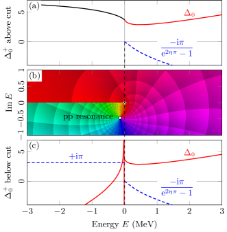
Figure 8: (Color online) Proton-proton function $\displaystyle\Delta^{+}_{0}(E)$ (b) in the complex $\displaystyle E$-plane, (a) on the real $\displaystyle E$-axis in the physical sheet and (c) in the unphysical sheet. The function is real for $\displaystyle\arg E=+\pi$. Its real part reduces to $\displaystyle\Delta_{0}(E)$ at $\displaystyle E>0$. In (c), the Coulomb poles at $\displaystyle\arg E=-\pi$ are indistinguishable at this scale.

As discussed in Sec. III.3, the function $\displaystyle\Delta^{+}_{0}(E)$ features zeroes corresponding to poles of the $\displaystyle S_{0}$ matrix element. Indeed, one notices a zero in Fig. 8(b) located at

$$E_{\rm res,pp}\simeq(-142-467\,\mathrm{i})~{}\mathrm{keV}\>,$$ (82)

that coincides with the proton-proton broad resonance referred to in literature Kok (1980); Mukhamedzhanov et al. (2010). Other nontrivial zeroes exist in the unphysical sheet at low negative energies ($\displaystyle\left|E\right|<1~{}\mathrm{Ry}$), but, being very close to the negative $\displaystyle E$-axis, they are interpreted in Ref. Kok (1980) as antibound states.

Furthermore, $\displaystyle\Delta^{+}_{0}(E)$ is smooth in the physical sheet near $\displaystyle E=0$, although it might be unclear in Fig. 8(a). In fact, the function has a inflection point at about $\displaystyle E=1.1~{}\mathrm{Ry}=13.9~{}\mathrm{keV}$ very close to the origin at this scale, hence the impression of an angular point at $\displaystyle E=0$.

The potential interest of $\displaystyle\Delta^{+}_{0}(E)$ to extrapolate experimental data to negative energies in the physical sheet is obvious in Fig. 8(a). Even though the essential singularity at $\displaystyle E=0$ prevents the interpolation functions from converging everywhere in the $\displaystyle E$-plane.

IV.1.3 Proton-proton usual effective-range function

The last function to show for the proton-proton ${}^{1}S_{0}$ wave is the traditional ERF $\displaystyle\varkappa_{0}(E)$. It is plotted in the complex $\displaystyle E$-plane in Fig. 9.

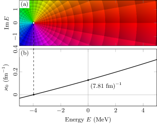
Figure 9: (Color online) Standard ERF $\displaystyle\varkappa_{0}(E)$ for the proton-proton ${}^{1}S_{0}$ collision (a) in the complex $\displaystyle E$-plane and (b) on the real $\displaystyle E$-axis. The zero is located at about $\displaystyle E\simeq-3.8~{}\mathrm{MeV}$.

The function $\displaystyle\varkappa_{0}(E)$ is real valued at both positive and negative energy, and it is analytic at $\displaystyle E=0$. Remarkably, in the two-proton scattering, $\displaystyle\varkappa_{0}(E)$ is a nearly straight line because the experimentally observed $\displaystyle\operatorname{\mathcal{O}}(E^{2})$ term is very small Landau and Smorodinsky (1944); Bethe (1949); Blatt (1948); Chew and Goldberger (1949); Jackson and Blatt (1950); Kok (1980).

The negative-energy zero of $\displaystyle\varkappa_{0}(E)$ shown in Fig. 9 is located at about

$$E=\frac{\hbar^{2}}{2m}\frac{2}{\alpha_{0}r_{0}}\simeq-3.8~{}\mathrm{MeV}\>,$$ (83)

using the linear approximation of the usual ERF, and the parameters from Eq. (80).

All these features justify the method based on the traditional ERF expansion, especially for light particles such as protons. Indeed, the low-energy behavior of the proton-proton ${}^{1}S_{0}$ phase shift is accurately given over a few MeVs by merely two parameters $\displaystyle\alpha_{0}$ and $\displaystyle r_{0}$.

IV.2 Use of the reduced effective-range function

In this section, we consider using the reduced ERF $\displaystyle\Delta_{0}(E)$ directly to obtain information on negative energies, as proposed in Ref. Ramírez Suárez and Sparenberg (2017). The proton-proton ${}^{1}S_{0}$ scattering is still used as a practical example.

The following results can still be compared to other scattering systems provided that we refer to the nuclear Rydberg energy. Indeed, this quantity governs most of the orders of magnitude of energy in the charged-particle scattering. This is why energies are expressed in $\displaystyle\mathrm{Ry}$ hereafter.

IV.2.1 Extraction of resonances

First, we focus on the determination of the proton-proton resonance from experimental data using the function $\displaystyle\Delta_{0}(E)$. For this purpose, we interpolate directly $\displaystyle\Delta_{0}(E)$ with Padé approximants of different orders, as done in Ref. Ramírez Suárez and Sparenberg (2017).

To compute the fitting, 120 data points sampled logarithmically are taken from the square-well model in the range $\displaystyle[10,10^{3}]~{}\mathrm{Ry}\simeq[0.125,12.5]~{}\mathrm{MeV}$. This range has been chosen because it is the closest to the experimental framework of proton-proton collision. The resulting Padé approximants of orders $\displaystyle[2/1]$, $\displaystyle[4/3]$ and $\displaystyle[6/5]$ are shown in Fig. 10(a). Our choice of the orders $\displaystyle[(n+1)/n]$ builds on the Refs. Hartt (1981); Midya et al. (2015), but different orders do not affect our results.

To get the resonance, one has to find the root of the equation $\displaystyle\cot\delta^{\mathrm{fit}}_{0}(E)=\mathrm{i}$, that is to say in terms of $\displaystyle\Delta_{0}(E)$

$$\Delta^{\mathrm{fit}}_{0}(E)=\frac{\mathrm{i}\pi}{\mathop{}\!\mathrm{e}^{2\eta\pi}-1}\>.$$ (84)

Solving Eq. (84) numerically with the Padé approximant $\displaystyle[6/5]$ provides a broad resonance at

$$E_{\rm res,pp}\simeq(-141-467\,\mathrm{i})~{}\mathrm{keV}\>,$$ (85)

very close to (82) that we have found in the square-well model, and previously reported in Refs. Mukhamedzhanov et al. (2010); Kok (1980). Such an agreement can be explained by the remoteness of the resonance pole from the nuclear Rydberg energy ($\displaystyle 1~{}\mathrm{Ry}\simeq 12.5~{}\mathrm{keV}$) below which the essential singularity of $\displaystyle\Delta_{0}(E)$ hinders the convergence of the interpolations, as shown in Fig. 10(a). In addition, being of modulus $\displaystyle\left|E_{\rm pp,res}\right|=0.488~{}\mathrm{MeV}$, the pole lies in a ring centered at $\displaystyle E=0$ that covers the data points in $\displaystyle[0.125,12.5]~{}\mathrm{MeV}$. Therefore, the fitting successfully provides the resonance pole, although no convergence of the Padé approximant is observed because of the logarithmic branch cut of $\displaystyle\Delta_{0}(E)$. Heuristically, the region of the complex $\displaystyle E$-plane where the fitting is reliable turns out to be the sector $\displaystyle\left|\arg E\right|\lesssim 3\pi/4$ and $\displaystyle\left|E\right|\gtrsim 1~{}\mathrm{Ry}$. Closer to the negative $\displaystyle E$-axis, spurious poles makes the fitting unusable.

Finally, we conclude that it is possible to extract narrow or broad resonances from the reduced ERF $\displaystyle\Delta_{0}(E)$, provided that the corresponding sought poles are not too close to the negative $\displaystyle E$-axis with respect to the nuclear Rydberg energy.

IV.2.2 Extrapolation to negative energies

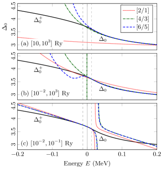
Figure 10: Interpolations of $\displaystyle\Delta_{0}(E)$ at $\displaystyle E>0$ for the proton-proton ${}^{1}S_{0}$ wave with Padé approximants of orders $\displaystyle[2/1]$, $\displaystyle[4/3]$ and $\displaystyle[6/5]$. $\displaystyle\Delta_{0}(E)$ is sampled logarithmically in 120 points (not shown) on different ranges (a) $\displaystyle[10,10^{3}]~{}\mathrm{Ry}$, (b) $\displaystyle[10^{-2},10^{3}]~{}\mathrm{Ry}$, and (c) $\displaystyle[10^{-2},10^{-1}]~{}\mathrm{Ry}$. The Coulomb range $\displaystyle[-1,1]~{}\mathrm{Ry}$ is surrounded by vertical dashed lines. The real part of $\displaystyle\Delta^{+}_{0}(E)$ (for $\displaystyle\arg E=+\pi$) is shown in solid black.

Now, we consider using the function $\displaystyle\Delta_{0}(E)$ to extract information on the bound states. Although the two-proton system has no bound state, it is useful to study how the interpolation of $\displaystyle\Delta_{0}(E)$ may extend to negative energies, especially, in which circumstances it approaches the function $\displaystyle\Delta^{+}_{0}(E)$, as predicted in Eq. (74).

As previously, we take 120 sample points of $\displaystyle\Delta_{0}(E)$ computed in the square-well model to fit the Padé approximants. Three sampling intervals are envisioned to reproduce different experimental situations. Case (a) is the typical situation encountered for proton-proton collision: no experimental data is known below about $\displaystyle 10~{}\mathrm{Ry}\simeq 0.125~{}\mathrm{MeV}$. Case (c) is more likely encountered with heavy or moderately heavy nuclei, for which the Rydberg energy is relatively high compared to nuclear energies. Case (b) is intermediate because involving both low and high energy data with respect to the Rydberg energy.

In case (a), 120 data points are sampled in the interval $\displaystyle[10,1000]~{}\mathrm{Ry}\simeq[0.125,12.5]~{}\mathrm{MeV}$. One notices in Fig. 10(a) that none of the Padé approximants is reliable in the Coulomb range, i.e., below $\displaystyle 1~{}\mathrm{Ry}$. The high-order Padé approximants $\displaystyle[4/3]$ and $\displaystyle[6/5]$ diverge near the inflection point located at about $\displaystyle 1.1~{}\mathrm{Ry}$. Beyond that point, spurious poles appear at negative energy (not visible in Fig. 10). This means that the $\displaystyle\Delta_{0}$-based extrapolation is not indicated for light particle systems such as protons.

In case (b), we consider a fictitious situation with 120 data points in the interval $\displaystyle[0.01,1000]~{}\mathrm{Ry}$. Although the Padé approximants are closer to $\displaystyle\Delta^{+}_{0}(E)$, they still diverge at negative energy. In addition, the Padé approximant $\displaystyle[4/3]$ shows a spurious pole very close to $\displaystyle E=0$ in the negative-energy Coulomb range. Such spurious poles are likely due to the negative-energy branch cut of $\displaystyle\Delta_{0}(E)$ which prevents the approximants from converging. From this point of view, additional data are not helpful and create more constraints that the Padé approximants cannot follow anyway.

Finally, in case (c), 120 data points are sampled in $\displaystyle[0.01,0.1]~{}\mathrm{Ry}\simeq[0.125,1.25]~{}\mathrm{keV}$. Interestingly, the fitted Padé approximants are significantly closer to $\displaystyle\Delta^{+}_{0}(E)$ up to about $\displaystyle-2~{}\mathrm{Ry}$.

Spurious poles at positive energy in case (c) make the Padé approximants unusable for $\displaystyle E\gtrsim 1~{}\mathrm{Ry}$. This seems to show that, in general, one has to choose between fitting at higher or lower energies than about $\displaystyle 1~{}\mathrm{Ry}$.

The Padé approximants in (c) are also consistent with each other although they do not seem to converge. Such an adequacy can be interpreted as the consequence of the asymptotic expansion (73) of $\displaystyle h^{+}_{0}(\eta)$. Furthermore, Fig. 10(c) shows that the $\displaystyle\Delta_{0}$-based extrapolation provides reliable results as long as enough experimental points are known in the Coulomb range. Since this condition is generally satisfied with heavy and moderately nuclei, the direct fitting of $\displaystyle\Delta_{0}(E)$ is useful for the analysis of weakly bound states. For instance, in case (c), bound states would correspond to negative-energy zeroes of $\displaystyle\Delta^{\mathrm{fit}}_{0}(E)$.

V Conclusions

In this paper, the effective-range function method for charged particles has been studied as well as recently proposed variants Ramírez Suárez and Sparenberg (2017); Blokhintsev et al. (2017a, b). The usual ERF method, due to Landau Landau and Smorodinsky (1944) and Bethe Bethe (1949), allows us to interpolate the experimental phase shifts at low energy with a minimum of fitting parameters. In this way, positive energy data can be extrapolated to the complex $\displaystyle E$-plane to determine resonances and bound states.

We have given a detailed proof of the expression of the usual ERF by a novel approach solely involving the properties of the Coulomb wave functions in the $\displaystyle E$-plane. We have established the connection between the original writing (50) of the ERF and the alternate formulation (65) due to Cornille and Martin Cornille and Martin (1962) and Hamilton et al. Hamilton et al. (1973) based on the function $\displaystyle h^{+}_{\ell}(\eta)$. We have also shown that the reduced ERF $\displaystyle\Delta_{\ell}$ Ramírez Suárez and Sparenberg (2017) has special structures at negative energy: an accumulation point of poles and zeroes as well as a branch cut emanating from the principal-valued logarithm. These structures, also seen in the complementary function $\displaystyle g_{\ell}(\eta)$, make the reduced ERF $\displaystyle\Delta_{\ell}$ singular at $\displaystyle E=0$. We have graphically verified the expected properties of the functions $\displaystyle\Delta_{\ell}$ and $\displaystyle\Delta^{+}_{\ell}$ in the $\displaystyle E$-plane for the well-known proton-proton ${}^{1}S_{0}$ collision.

As pointed out in Ref. Ramírez Suárez and Sparenberg (2017), the function $\displaystyle\Delta_{\ell}$ is in practice much smaller than $\displaystyle g_{\ell}(\eta)$ for heavy and moderately heavy nuclei at low energy, because of the prefactor $\displaystyle\pi/(\mathop{}\!\mathrm{e}^{2\eta\pi}-1)$. Therefore, the addition of $\displaystyle g_{\ell}(\eta)$ could bias the heuristic interpolation of the usual ERF $\displaystyle\varkappa_{\ell}$, leading to an underfitting of the phase-shift-dependent part $\displaystyle\Delta_{\ell}$ Orlov et al. (2016, 2017). To avoid this, we propose to interpolate $\displaystyle\Delta_{\ell}$ by means of Eq. (71) considering $\displaystyle-g_{\ell}(\eta)$ as the first term of the expansion, in accordance with the usual ERF theory.

A potential alternative proposed in Ref. Ramírez Suárez and Sparenberg (2017) is to directly interpolate $\displaystyle\Delta_{\ell}$ by Padé approximants, being closer to the phase shift. Caution should be exercised when using this method because the Padé approximants are not expected to faithfully converge to the function $\displaystyle\Delta_{\ell}$, given its singularities.

However, this approach turns out to be heuristically useful in two different cases: either to determine resonances, or to study weakly bound states ($\displaystyle\lesssim 1~{}\mathrm{Ry}$), as long as data are known in appropriate energy ranges. With bound states, the method exploits the noticeable property that $\displaystyle\Delta_{\ell}$ and $\displaystyle\Delta^{+}_{\ell}$ join smoothly together at $\displaystyle E=0$ in the physical sheet, due to the common asymptotic Stirling expansion of $\displaystyle g_{\ell}(\eta)$ and $\displaystyle h^{+}_{\ell}(\eta)$ at this point. This property allows us to reliably extrapolate data below $\displaystyle 1~{}\mathrm{Ry}$ to negative energy in $\displaystyle\left|E\right|\lesssim 1~{}\mathrm{Ry}$ in the physical sheet with expansions of relatively low order. In practice, obtaining a reliable interpolation on the two ranges $\displaystyle E\ll 1~{}\mathrm{Ry}$ and $\displaystyle E\gg 1~{}\mathrm{Ry}$ turns out to be difficult, likely because of the sharp inflection point of $\displaystyle\Delta_{\ell}$ at $\displaystyle E\simeq 1.1~{}\mathrm{Ry}$. For this reason, it seems preferable to restrict the data points to specific energy ranges when fitting the Padé approximants.

Finally, the present study theoretically justifies in which situations the low-energy scattering of charged particles can be directly parametrized in terms of a Taylor or Padé expansion of the $\displaystyle\Delta_{\ell}$ function, as was empirically found for the $\displaystyle{}^{12}\mathrm{C}+\alpha$ system Ramírez Suárez and Sparenberg (2017); Blokhintsev et al. (2017a, b). For other systems, like proton-proton, the use of the standard ERF is still required, at least to compensate for the lack of experimental data at energies around and below the nuclear Rydberg energy, where the mathematical singularities of the Coulomb functions play an crucial role. With these guidelines in mind, other systems can be tackled.

In the future, we plan to further study the interest of Padé approximants, for either the reduced or the standard effective-range functions, to extend the parametrization studied here for low-energy data up to high energies. We also plan to expand the present results to other reaction channels and to coupled-channel situations.

Appendix A Graphing complex functions

Graphical representation of complex-valued functions of one complex variable ($\displaystyle f:\mathbb{C}\rightarrow\mathbb{C}$) are quite challenging. Although there are many ways to proceed, we have chosen in this paper to use color-coded phase plots, as recommended in Ref. Wegert (2012). This method is more straightforward to implement and provides less ambiguous graphics than 3D plots Wegert (2012), with the functions that we consider. However, for convenience, the complementary 2D plots along the real axis are shown throughout this paper.

This graphical method consists in representing the complex argument with a hue on the color wheel. Indeed, the argument turns out to be more useful than the complex modulus to identify the analytic structure of a function, especially the poles, zeroes and branch cuts. In practice, poles can be graphically distinguished from zeroes using Cauchy’s argument principle Wegert (2012).

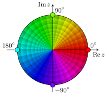
Figure 11: (Color online) Identity function in the complex plane with the color code used in this paper. The complex argument is represented with a hue: red color at $\displaystyle 0^{\circ}$ (for $\displaystyle\mathbb{R}^{+}$), chartreuse green at $\displaystyle 90^{\circ}$, cyan at $\displaystyle 180^{\circ}$ (for $\displaystyle\mathbb{R}^{-}$) and violet at $\displaystyle-90^{\circ}$. The log-polar grid highlights both the modulus and the argument.

The color map used in this paper is shown in Fig. 11 for the identity function $\displaystyle z\mapsto z$. The analytic structures are also highlighted by an array of contour lines in phase and in modulus forming a logarithmic polar grid. This logarithmic polar grid allows us to directly visualize the conformality of the mapping $\displaystyle z\mapsto f(z)$ — and therefore the analyticity of $\displaystyle f(z)$ — through the preservation of right angles of the tiles Wegert (2012). In practice, the polar grid is obtained by modulation of the color value $\displaystyle v(z)$ according to the formula

$$v(z)=v_{0}+(1-v_{0})\frac{\operatorname{frac}\big{(}\frac{N}{2\pi}\ln\left|z\right|\big{)}+\operatorname{frac}\big{(}\frac{N}{2\pi}\arg z\big{)}}{2}\>,$$ (86)

where $\displaystyle\operatorname{frac}{x}$ denotes the fractional part, also known as the sawtooth function, defined by $\displaystyle\operatorname{frac}{x}=x-\lfloor x\rfloor$ with the floor function $\displaystyle x\mapsto\lfloor x\rfloor$. We have chosen to set the minimum color value $\displaystyle v_{0}$ to $\displaystyle 60\%$ and the number of angular divisions $\displaystyle N$ to $\displaystyle 32$.

Many other color codes can produce such a polar grid, but Eq. (86) has the advantage of not requiring too much extra computing effort, and ensuring for all $\displaystyle N$ that the sides of the tiles look as equal as possible, independently of the modulus.

References

- Bethe (1949) H. A. Bethe, Phys. Rev. 76, 38 (1949).
- Landau and Smorodinsky (1944) L. D. Landau and Y. A. Smorodinsky, J. Phys. USSR 8, 154 (1944).
- Blatt (1948) J. M. Blatt, Phys. Rev. 74, 92 (1948).
- Chew and Goldberger (1949) G. F. Chew and M. L. Goldberger, Phys. Rev. 75, 1637 (1949).
- Jackson and Blatt (1950) J. D. Jackson and J. M. Blatt, Rev. Mod. Phys. 22, 77 (1950).
- Joachain (1979) C. J. Joachain, Quantum Collision Theory, 2nd ed. (North-Holland, Amsterdam, 1979).
- Newton (1982) R. G. Newton, Scattering Theory of Waves and Particles, 2nd ed., Dover Books on Physics (Dover, Mineola, New York, 1982).
- van Haeringen (1985) H. van Haeringen, Charged Particle Interactions: Theory and Formulas (Coulomb Press, Leiden, 1985).
- Hartt (1981) K. Hartt, Phys. Rev. C 23, 2399 (1981).
- Rakityansky and Elander (2013) S. A. Rakityansky and N. Elander, J. Math. Phys. 54, 122112 (2013).
- Midya et al. (2015) B. Midya, J. Evrard, S. Abramowicz, O. L. Ramírez Suárez, and J.-M. Sparenberg, Phys. Rev. C 91, 054004 (2015).
- Abramowitz and Stegun (1964) M. Abramowitz and I. A. Stegun, Handbook of Mathematical Functions: With Formulas, Graphs, and Mathematical Tables, Dover Books on Mathematics (Dover, New York, 1964).
- Olver et al. (2010) F. W. J. Olver, D. W. Lozier, R. F. Boisvert, and C. W. Clark, NIST Handbook of Mathematical Functions, 1st ed. (NIST, New York, 2010).
- Cornille and Martin (1962) H. Cornille and A. Martin, Il Nuovo Cimento 26, 298 (1962).
- Lambert (1969) E. Lambert, Helv. Phys. Acta 42, 667 (1969).
- Hamilton et al. (1973) J. Hamilton, I. Øverbö, and B. Tromborg, Nucl. Phys. B 60, 443 (1973).
- van Haeringen and Kok (1982) H. van Haeringen and L. P. Kok, Phys. Rev. A 26, 1218 (1982).
- Humblet (1990) J. Humblet, Phys. Rev. C 42, 1582 (1990).
- Yarmukhamedov and Baye (2011) R. Yarmukhamedov and D. Baye, Phys. Rev. C 84, 024603 (2011).
- Ramírez Suárez and Sparenberg (2017) O. L. Ramírez Suárez and J.-M. Sparenberg, Phys. Rev. C 96, 034601 (2017).
- Blokhintsev et al. (2017a) L. D. Blokhintsev, A. S. Kadyrov, A. M. Mukhamedzhanov, and D. A. Savin, Phys. Rev. C 95, 044618 (2017a).
- Blokhintsev et al. (2017b) L. D. Blokhintsev, A. S. Kadyrov, A. M. Mukhamedzhanov, and D. A. Savin, “Extrapolation of scattering data to the negative-energy region II,” (2017b), arXiv preprint, arXiv:1710.10767v1 [nucl-th] .
- Orlov et al. (2016) Y. V. Orlov, B. F. Irgaziev, and L. I. Nikitina, Phys. Rev. C 93, 014612 (2016).
- Orlov et al. (2017) Y. V. Orlov, B. F. Irgaziev, and J.-U. Nabi, Phys. Rev. C 96, 025809 (2017).
- Naisse (1977) J. P. Naisse, Nucl. Phys. A 278, 506 (1977).
- Kok (1980) L. P. Kok, Phys. Rev. Lett. 45, 427 (1980).
- Bergervoet et al. (1988) J. R. Bergervoet, P. C. van Campen, W. A. van der Sanden, and J. J. de Swart, Phys. Rev. C 38, 15 (1988).
- Mukhamedzhanov et al. (2010) A. M. Mukhamedzhanov, B. F. Irgaziev, V. Z. Goldberg, Y. V. Orlov, and I. Qazi, Phys. Rev. C 81, 054314 (2010).
- Chen et al. (1989) C. R. Chen, G. L. Payne, J. L. Friar, and B. F. Gibson, Phys. Rev. C 39, 1261 (1989).
- Kievsky et al. (1997) A. Kievsky, S. Rosati, M. Viviani, C. R. Brune, H. J. Karwowski, E. J. Ludwig, and M. H. Wood, Phys. Lett. B 406, 292 (1997).
- Brune et al. (2001) C. R. Brune, W. H. Geist, H. J. Karwowski, E. J. Ludwig, K. D. Veal, M. H. Wood, A. Kievsky, S. Rosati, and M. Viviani, Phys. Rev. C 63, 044013 (2001).
- Humblet et al. (1976) J. Humblet, P. Dyer, and B. A. Zimmerman, Nucl. Phys. A 271, 210 (1976).
- Brune et al. (1999) C. R. Brune, W. H. Geist, R. W. Kavanagh, and K. D. Veal, Phys. Rev. Lett. 83, 4025 (1999).
- Filippone et al. (1989) B. W. Filippone, J. Humblet, and K. Langanke, Phys. Rev. C 40, 515 (1989).
- Mohr et al. (2016) P. J. Mohr, D. B. Newell, and B. N. Taylor, J. Phys. Chem. Ref. Data 45, 043102 (2016).
- Breit et al. (1936) G. Breit, E. U. Condon, and R. D. Present, Phys. Rev. 50, 825 (1936).
- Messiah (1961) A. Messiah, Quantum Mechanics, Vol. 1 (Interscience, New York, 1961).
- Gottfried (1966) K. Gottfried, Quantum Mechanics: Volume I: Fundamentals (W. A. Benjamin, New York, 1966).
- Bateman et al. (1953) H. Bateman, A. Erdélyi, W. Magnus, F. Oberhettinger, and F. G. Tricomi, Higher Transcendental Functions, Vol. 1 (McGraw-Hill, New York, 1953).
- Humblet (1984) J. Humblet, Ann. Phys. (NY) 155, 461 (1984).
- Yost et al. (1936) F. L. Yost, J. A. Wheeler, and G. Breit, Phys. Rev. 49, 174 (1936).
- Kummer (1837) E. E. Kummer, J. Reine Angew. Math. 17, 228 (1837), written in Latin.
- Hamming (1973) R. W. Hamming, Numerical Methods for Scientists and Engineers, 2nd ed., Dover Books on Engineering (Dover, New York, 1973).
- Albeverio et al. (1988) S. Albeverio, F. Gesztesy, R. Høegh-Krohn, and H. Holden, Solvable Models in Quantum Mechanics, edited by W. Beiglböck, J. L. Birman, R. P. Geroch, E. H. Lieb, T. Regge, and W. Thirring, Texts and Monographs in Physics (Springer, New York, 1988).
- Wolfram (1999) S. Wolfram, The Mathematica® Book, 4th ed. (Cambridge University, New York, 1999).
- Wegert (2012) E. Wegert, Visual Complex Functions: An Introduction with Phase Portraits (Birkhäuser, Basel, 2012).