Iterative Refinement of A Modified Lavrentiev Regularization Method for De-convolution of the Discrete Helmholtz Type Differential Filter

Abstract.

We propose and analyze an iterative refinement of a modified Lavrentiev regularization method for deconvolution of the discrete Helmholtz-type differential filter. The modification for the Lavrentiev regularization method exploits the properties of the Helmholtz filter, and we prove that the modification reduces the error bound between the original solution and the approximated solution. Furthermore, we derive an optimal stopping condition on the number of iterations necessary for the regularization. We provide numerical examples demonstrating the benefits of this iterative modified Lavrentiev regularization over a family of Tikhonov regularization methods.

1. Introduction

Since its introduction in $1963$, Large Eddy Simulation (LES), a model in between the direct simulation of the Navier-Stokes equations (DNS) and Reynolds-averaged Navier-Stokes equations (RANS), has been widely applied in meteorology, astrophysics, aerospace, mechanical, chemical and environmental engineering [24, 11, 23, 29, 6, 25, 27]. With a certain low-pass filter, LES is able to reduce the spatial scales (and sometimes even the temporal scales), therefore reducing the computational load of doing DNS [27, 12, 18, 3]. Most LES filters use convolution, defined as follows,

(1) $$\bar{u}(x;\delta)=\int_{x^{\prime}\in\Omega}G(x-x^{\prime};\delta)u(x^{\prime})\,dx^{\prime}$$

where $\Omega$ is the spatial domain, and $\delta$ is the filtering radius (also known as the length scale cutoff) [10, 27, 12, 9]. However the LES filter we are interested in uses a Helmholtz-type differential equation. In this paper, we will address the issue on how to deconvolve this Helmholtz filter so that we can resolve the smaller length scales below the spatial cutoff, $\delta$. We are given a Helmholtz filter $G$ and a filtered solution $\bar{u}$, where $Gu=\bar{u}$ with $u$ being the desired solution, then we will use an iterative regularization algorithm to find an approximation $\tilde{u}$, such that $\tilde{u}\approx u$, and the error, $u-\tilde{u}$, is well contained. The mathematical definition of the filtering process is given as follows,

Problem 1.1 (Noise Free Model Problem).

Let $X$ and $Y$ be Hilbert spaces. Given a linear filter operator $G:X\rightarrow Y$ and a filtered signal $\bar{u}\in\text{Range}(G)$. The noise free model problem is to find $u\in X$ which satisfies

(2) $$Gu=\bar{u}.$$

Problem 1.2 (Noisy Model Problem).

Let $X$ and $Y$ be Hilbert spaces. Given a linear filter operator $G:X\rightarrow Y$ and a filtered signal $\bar{u}\in\text{Range}(G)$ and noise $\epsilon\in Y$. The noisy model problem is to find $u\in X$ satisfying

(3) $$Gu=\bar{u}+\epsilon.$$

We will mainly consider the case where the linear filter $G$ is a Helmholtz filter, hence solving either Problem 1.1 or Problem 1.2 becomes a deconvolution problem. This kind of deconvolution problem is an important inverse problem [9, 16, 21, 22, 30]. This problem occurs in many applications including parameter identification [7, 8], the deconvolution problem of image processing [4], and the closure problem in turbulence modeling [3, 10, 18, 22]. The deconvolution problem gets more complicated when noise is present in the filtering process. It is known that if $G$ is compact and $Range(G)$ is infinite dimensional, then Problems 1.1 and 1.2 are ill-posed [1, 2, 13, 26, 28, 35, 33]. Tikhonov-Lavrentiev regularization, a regularization method described further in Algorithm 2.8, which introduces a regularization parameter $\alpha$, is a well-established method used to solve Problems 1.1 and 1.2 [22, 19, 15, 8, 34]. However, Tikhonov-Lavrentiev regularization is a general method which does not exploit the properties of the Helmholtz-type differential filter (with filtering radius $\delta$). Therefore we introduce a new regularization method with a modification to iterative Tikhonov-Lavrentiev regularization, which in Theorem 3.8 shows that it is able to exploit the properties of the Helmholtz filter $G$ and improves the error bounds for Problems 1.1. That is, a small algorithmic modification leads to a large improvement in the error bounds.

In section 2, we introduce the necessary notation and inequalities which are used in the proofs of our theorems. Section 3 describes the Modified Iterative Tikhonov-Lavrentiev Regularization (Mitlar) algorithm in details and shows the error bounds in both the continuous case and discrete case. Section 4 provides an optimal stopping condition for the total number of iterations to counter the presence of noise in the the filtering process. Finally, in section 5, we show a number of numerical examples to verify the convergence rate, the optimal stopping condition and also compare the performance of our new algorithm to a family of existing Tikhonov-Lavrentiev regularization methods: original Tikhonov-Lavrentiev regularization, iterative Tikhonov-Lavrentiev regularization, and modified Tikhonov-Lavrentiev regularization.

2. Preliminaries and notation

Throughout this paper, we use the standard notation for Lebesgue and Sobolev spaces and their norms. Also, $\Omega$ will be a regular, bounded, polyhedral domain in $\mathbb{R}^{n}$. We define the following space

(4) $$X=H^{1}_{0}(\Omega)^{d}=\left\{v\in L^{2}(\Omega)^{d}:\nabla v\in L^{2}(\Omega)^{d\times d}\text{ and }v=0\text{ on }\partial\Omega\right\}.$$

The norm $\|\cdot\|$ (when subscript is not present) will also denote the $L^{2}(\Omega)$ norm unless otherwise specified in a proof. Similarly the inner product $(\cdot,\cdot)$ will denote the $L^{2}(\Omega)$ inner product. We will use the notation $X^{h}\subset X$ to denote a finite dimensional subset of $X$. An example of $X^{h}$ is the set of continuous polynomials of degree $k$. We also assume that we have homogeneous boundary data throughout. We use the following approximation inequalities, see [5],

$$\inf_{v\in X^{h}}\|u-v\|_{L^{2}(\Omega)} \leq Ch^{k+1}\|u\|_{H^{k+1}(\Omega)},\quad u\in H^{k+1}(\Omega)^{n},$$

(5) $$\inf_{v\in X^{h}}\|u-v\|_{H^{1}(\Omega)} \leq Ch^{k}\|u\|_{H^{k}(\Omega)},\quad u\in H^{k+1}(\Omega)^{n}.$$

Other well known inequalities used herein include:

• Cauchy-Schwartz inequality: $|(f,g)|\leq\|f\|\|g\|,\quad\forall f,g\in L^{2}(\Omega)$.

• Young’s inequality: $ab\leq\frac{\epsilon}{p}a^{p}+\frac{\epsilon^{-q/p}}{q}b^{q}$, where $1<p,q<\infty$, $\frac{1}{p}+\frac{1}{q}=1$, $\epsilon>0$, and $a,b\geq 0$.

• Poincare-Friedrich’s inequality: $\|v\|\leq C_{PF}\|\nabla v\|,\quad\forall v\in X$.

• Triangle inequality: $\|a+b\|\leq\|a\|+\|b\|$.

2.1. The differential filter

The differential filter (also known as the Helmholtz-type differential filter) is used in multiple large eddy simulation models [3, 9, 10, 18, 21, 22]. This filter is equivalent to the Pao filter used in image processing [18].

Definition 2.1 (Differential filter).

The differential filter $G$ is defined as $Gu=\bar{u}$, where $u$ and $\bar{u}$ satisfy

(6) $$-\delta^{2}\Delta\bar{u}+\bar{u}=u\quad\text{ in }\Omega.$$

Remark 2.2 (Variational differential filter).

The differential filter is equivalent (see [21, 22]) to the following variational formulation. Find $\overline{u}\in H^{1}_{0}(\Omega)$ satisfying

(7) $$\delta^{2}(\nabla\overline{u},\nabla v)+(\overline{u},v)=(u,v),\quad\forall v\in X.$$

Definition 2.3 (Discrete differential filter).

Let $X^{h}$ be a finite dimensional subspace of $X$. We define $G^{h}:L^{2}(\Omega)^{d}\rightarrow X^{h}$ where $\overline{u}^{h}=G^{h}u$ which is the unique solution in $X^{h}$ to

(8) $$\delta^{2}\left({\nabla\overline{u}^{h},\nabla v^{h}}\right)+\left({\overline{u}^{h},v^{h}}\right)=\left({u,v^{h}}\right),\quad\forall v^{h}\in X^{h}.$$

Lemmas 2.4, 2.5, 2.6, and 2.7 are quoted from [21] for completeness.

Lemma 2.4.

If $u\in L^{2}(\Omega)^{d}$, the following stability estimate for problem (7) holds:

(9) $$\delta^{2}\|\nabla\overline{u}\|^{2}+\frac{1}{2}\|\overline{u}\|^{2}\leq\frac{1}{2}\|u\|^{2}.$$

Lemma 2.5.

The operator $G:L^{2}(\Omega)^{d}\rightarrow X$ is self-adjoint.

Lemma 2.6.

If $\nabla u\in L^{2}(\Omega)^{d}$ and $\overline{u}$ satisfies (7), then

(10) $$\frac{\delta^{2}}{2}\|\nabla(u-\overline{u})\|^{2}+\|u-\overline{u}\|^{2}\leq\frac{\delta^{2}}{2}\|\nabla u\|^{2}.$$

If, additionally $\Delta u\in L^{2}(\Omega)^{d}$, then

(11) $$\delta^{2}\|\nabla(u-\overline{u})\|^{2}+\frac{1}{2}\|u-\overline{u}\|^{2}\leq\delta^{4}\|\Delta u\|^{2}.$$

Lemma 2.7.

The operator $G^{h}:L^{2}(\Omega)^{d}\rightarrow X^{h}$ is self-adjoint and positive semi-definite on $L^{2}(\Omega)$ and positive definite on $X^{h}$.

2.2. Tikhonov regularization

A major tool which is often used to solve inverse problems is the Tikhonov regularization [31, 32, 8]. In order to solve an ill-posed linear system $Gu=\bar{u}$, a general Tikhonov regularization will try to find the minimizer of the following problem,

(12) $$u_{T}=\underset{{u}}{\operatorname{argmin}}\{\left|\left|Gu-\bar{u}\right|\right|^{2}+\left|\left|\Gamma u\right|\right|^{2}\}$$

where $\Gamma$ is a suitably chosen linear operator, called Tikhonov operator (or Tikhonov matrix when $G$ is a matrix). The Tikhonov minimizer of (12), $u_{T}$, has a closed form expression,

(13) $$u_{T}=(G^{*}G+\Gamma^{*}\Gamma)^{-1}G^{*}u$$

where $G^{*}$ and $\Gamma^{*}$ are Hermitian transposes of $G$ and $\Gamma$ respectively. In most cases, $\Gamma$ is picked as a multiple of the identity operator, that is, $\Gamma=\alpha I$. In this case, (13) simplifies down to,

(14) $$u_{T}=(G^{*}G+\alpha^{2}I)^{-1}G^{*}u$$

If the operator $G$ is monotone, then instead of solving $Gu=\bar{u}$ with the the perturbed normal equation from Tikhonov regularization, Tikhonov-Lavrentiev regularization can be used. This is known in the literature as the method of Lavrentiev Regularization [17] or the method of Singular Perturbation [20],

Definition 2.8 (Tikhonov-Lavrentiev Regularization).

Choose a regularization parameter $\alpha>0$. Solve for $u_{0}$ satisfying

$$(G+\alpha I)u_{0} =\overline{u},\quad\text{in }\Omega.$$

This regularization method can be improved by an iterative method.

Definition 2.9 (Iterated Tikhonov-Lavrentiev regularization).

Choose a regularization parameter $\alpha>0$ and fix the number of updates $J\geq 1$. The iterative Tikhonov-Lavrentiev approximations $u_{j}$ $(0\leq j\leq J)$ are found by solving

$$(G+\alpha I)u_{0} =\overline{u},\quad\text{in }\Omega,$$

$$(G+\alpha I)(u_{j}-u_{j-1}) =\overline{u}-Gu_{j-1},\quad\text{in }\Omega.$$

Given a source condition, it is shown in [8, 15] that Tikhonov-Lavrentiev and iterative Tikhonov-Lavrentiev regularization converge to $u$ as $\alpha\rightarrow 0$ (in the noise free case) and as $\epsilon\rightarrow 0$ and $\alpha\rightarrow 0$ (in the noisy case).

Theorem 2.10 (Error bound of Tikhonov-Lavrentiev regularization).

Suppose that $G$ is non-negative definite. Fix $\alpha>0$. Let $e_{j}=u-u_{j}$ for all $j=0,\dots,J$. Suppose, for some $\beta\geq 0$ that $u\in Range(G^{\beta}$) and the noise is bounded $\|\epsilon\|\leq\epsilon_{0}<\infty$. Then, there exists a constant $C(J)<\infty$ such that, for any $0\leq J\leq\beta$,

(15) $$\|e_{J}\|\leq\frac{(J+1)\epsilon_{0}}{\alpha}+\alpha^{J+1}C(J).$$

Moreover, if $\alpha=\alpha(\epsilon_{0})=C\epsilon_{0}^{1/(J+2)}$ we have that $\|e_{J}\|\leq C\epsilon_{0}^{1-1/(J+2)}$.

The error bounds for Tikhonov-Lavrentiev regularization are similar to that of Tikhonov regularization, see [15, 8, 34].

3. Modification to iterative Tikhonov-Lavrentiev regularization

Algorithm 3.1 describes the modification which we add to iterative Tikhonov-Lavrentiev Regularization to develop our new algorithm, the Modified Iterative Tikhonov-Lavrentiev Regularization (Mitlar). We analyze the error in the continuous case by separating it into the following components: the regularization error in the Mitlar algorithm and the amount of noise amplification due to our regularization. We then discretize Mitlar in Algorithm 3.9. We analyze the error in the discretized case by separating it into the following components: the regularization error in the continuous Mitlar algorithm, the discretization error in the solution, and the discretized noise amplification due to the discrete Mitlar algorithm.

Algorithm 3.1.

(Modified Iterated Tikhonov-Lavrentiev Regularization [Mitlar]) Given the convolved data $\bar{u}$, to solve for $u$ satisfying $Gu=\bar{u}$ (the noise free model) or $Gu=\bar{u}+\epsilon$ (the noisy model), we fix the maximum number of iterations $J\geq 1$ and regularization parameter $\alpha>0$. Solve for $u_{0}$ satisfying

(16) $$[(1-\alpha)G+\alpha I]u_{0}=\bar{u}.$$

Then for $j=1,...,J$, solve for $u_{j}$ satisfying

(17) $$[(1-\alpha)G+\alpha I](u_{j}-u_{j-1})=\bar{u}-Gu_{j-1}.$$

We define the following regularization operators $D_{\alpha}$ and $D_{\alpha,j}$ for convenience of notation.

Definition 3.2.

For $\alpha>0$ define the modified Tikhonov-Lavrentiev operator $D_{\alpha}$ to be

(18) $$D_{\alpha}=[(1-\alpha)G+\alpha I]^{-1}.$$

For $j>0$, define the $j^{th}$ modified iterative Tikhonov-Lavrentiev operator $D_{\alpha,j}$ by

(19) $$D_{\alpha,j}\overline{u}=u_{j},$$

where $u_{j}$ is obtained via Algorithm 3.1.

Remark 3.3 (Variational formulation of Mitlar).

Assume $G$ is the differential filter defined in (7). Algorithm 3.1 is equivalent to the following variational formulation. Given $u\in L^{2}(\Omega)$, then $u_{J}=D_{J}\bar{u}$ is the unique solution to the following equations

(20) $$\alpha\delta^{2}\left({\nabla u_{0},\nabla v}\right)+\left({u_{0},v}\right) =\delta^{2}\left({\nabla\bar{u},\nabla v}\right)+\left({\bar{u},v}\right),\quad\forall v\in X,\text{ and}$$

$$\alpha\delta^{2}\left({\nabla u_{j},\nabla v}\right)+\left({u_{j},v}\right) =\delta^{2}\left({\nabla\bar{u},\nabla v}\right)+\left({\bar{u},v}\right)+\alpha\delta^{2}\left({\nabla u_{j-1},\nabla v}\right),\quad\forall v\in X.$$

Theorem 3.8 shows that this modification to Tikhonov-Lavrentiev regularization provides a higher order deconvolution error compared to iterated Tikhonov-Lavrentiev regularization. The following lemmas and propositions are needed for the proof of the error bound in Theorem 3.8.

Lemma 3.4.

For $0\leq\alpha\leq 1$, the function $f(x)=((1-\alpha)x+\alpha)^{-1}$ maps the interval $(0,1]$ to $[1,\frac{1}{\alpha})$, and the function $g(x)=x((1-\alpha)x+\alpha)^{-1}$ maps the interval $(0,1]$ to $(0,1]$.

Proof.

The term $(1-\alpha)x+\alpha$ is a convex combination of $x$ and $1$, so

$$\alpha<(1-\alpha)x+\alpha\leq 1,\text{ and}$$

$$1\leq\frac{1}{(1-\alpha)x+\alpha}<\frac{1}{\alpha}.$$

For the bounds on $g(x)$, consider

$$g^{\prime}(x)=\alpha((1-\alpha)x+\alpha)^{-2}.$$

So $g^{\prime}(x)$ has no critical points in the interval $(0,1)$. Therefore $g(x)$ attains its extrema on the boundary of $[0,1]$. Note that $g(1)=1$, and $g(x)=0$ if and only if $x=0$. Therefore $g:(0,1]\rightarrow(0,1]$. ∎

Lemma 3.5.

For $0\leq\alpha\leq 1$, the operators $D_{\alpha}$, $D_{\alpha}G$, and $I-D_{\alpha}G$ are bounded. In particular, they satisfy

(21) $$\|D_{\alpha}\|\leq\frac{1}{\alpha},\quad\|D_{\alpha}G\|\leq 1,\text{ and }\|I-D_{\alpha}G\|\leq 1.$$

Proof.

The method of proof is similar to that employed in [22]. The differential filter operator $G$ has a spectrum that lies in $(0,1]$. Therefore by Lemma 3.4, the spectrum of $D_{\alpha}=((1-\alpha)G+\alpha I)^{-1}$ lies between $[1,\frac{1}{\alpha})$. Also by Lemma 3.4, the spectrum of $D_{\alpha}G=((1-\alpha)G+\alpha I)^{-1}G$ lies between (0,1]. Similarly, the spectrum of $I-D_{\alpha}G$ lies between [0,1). ∎

Proposition 3.6.

The error equation $e_{J}=u-u_{J}$ is given by

(22) $$e_{J}=(-\alpha\delta^{2})^{J+1}(D_{\alpha}G)^{J+1}(\Delta^{J+1}u),$$

and the error is bounded

(23) $$\|e_{J}\|\leq(\alpha\delta^{2})^{J+1}\|\Delta^{J+1}u\|.$$

Proof.

For $0<j\leq J$, we start with (17) and an identity for the original solution $u$,

$$[(1-\alpha)G+\alpha I](u_{j}-u_{j-1}) =\bar{u}-Gu_{j-1}\quad\text{and}$$

$$[(1-\alpha)G+\alpha I](u-u) =\bar{u}-Gu.$$

Subtracting these equations and rearranging gives

(24) $$e_{j}=\alpha D_{\alpha}(I-G)e_{j-1}=\alpha D_{\alpha}G(G^{-1}-I)e_{j-1}.$$

For $j=0$, we use (16) and the true solution

$$[(1-\alpha)G+\alpha I]u_{0} =\bar{u}\quad\text{and}$$

$$[(1-\alpha)G+\alpha I]u =(1-\alpha)\bar{u}+\alpha u.$$

Subtraction gives

(25) $$e_{0}=\alpha D_{\alpha}(I-G)u=\alpha D_{\alpha}G(G^{-1}-I)u.$$

Thus, we arrive at,

$$e_{J}=\alpha^{J+1}(D_{\alpha}G)^{J+1}(G^{-1}-I)^{J+1}u$$

Using the fact that $(G^{-1}-I)u=-\delta^{2}\Delta u$, we have shown equation (22). The norm of the error is bounded by taking the norm of the error equation (22) and using the bound on $\|D_{\alpha}G\|$ in (21) to obtain

$$\|e_{J}\| =\|(-\alpha\delta^{2})^{J+1}(D_{\alpha}G)^{J+1}(\Delta^{J+1}u)\|$$

$$\leq(\alpha\delta^{2})^{J+1}\|(D_{\alpha}G)^{J+1}\|\|\Delta^{J+1}u\|$$

$$\leq(\alpha\delta^{2})^{J+1}\|\Delta^{J+1}u\|.$$

∎

Proposition 3.7.

The $j^{th}$ step of the Mitlar algorithm, $u_{j}$, is given by

(26) $$u_{j}:=D_{\alpha,j}\overline{u}=D_{\alpha}\sum_{i=0}^{j}(\alpha D_{\alpha}(I-G))^{i}\overline{u}.$$

Proof.

Starting with (17), solve for $u_{j}$ with the equations

$$I-D_{\alpha}G=\alpha D_{\alpha}(I-G)\text{ and }u_{0}=D_{\alpha}\overline{u}.$$

$$u_{j} =u_{j-1}+D_{\alpha}(\overline{u}-Gu_{j-1})$$

$$=D_{\alpha}\overline{u}+(I-D_{\alpha}G)u_{j-1}$$

$$=D_{\alpha}\overline{u}+\alpha D_{\alpha}(I-G)u_{j-1}$$

$$\vdots$$

$$=D_{\alpha}\sum_{i=0}^{j}(\alpha D_{\alpha}(I-G))^{i}\overline{u}.$$

as claimed. ∎

Noise amplification is one of the fundamental difficulties in solving ill-posed inverse problems [8]. The noise amplification is studied in Problem 1.2 where $\bar{u}$ has additive noise $\epsilon$. The Mitlar algorithm applied to this problem gives an improvement over iterated Tikhonov regularization in the noise free portion of the error as shown in Proposition 3.6. The bound on the error in the noisy data is no worse as shown in Theorem 3.8.

Theorem 3.8.

Under the conditions of Algorithm 3.1 and (6) and if there exists some $\epsilon_{0}$ such that $\|\epsilon\|<\epsilon_{0}$, then the error in the $j^{th}$ step of the Mitlar algorithm is

(27) $$e_{J}=(-\alpha\delta^{2})^{J+1}(D_{\alpha}G)^{J+1}(\Delta^{J+1}u)+D_{\alpha}\sum_{j=0}^{J}(I-D_{\alpha}G)^{j}\epsilon.$$

The error is bounded,

(28) $$\|e_{J}\|\leq(\alpha\delta^{2})^{J+1}\|\Delta^{J+1}u\|+\frac{(J+1)\epsilon_{0}}{\alpha}.$$

Proof.

Using the definition the $J^{th}$ modified iterative Tikhonov-Lavrentiev operator $D_{\alpha,J}$ and $Gu=\bar{u}+\epsilon$, we have

$$u_{J} =D_{\alpha,J}\overline{u}$$

$$=D_{\alpha,J}(Gu-\epsilon)$$

$$=D_{\alpha,J}Gu-D_{\alpha,J}\epsilon$$

We then divide the error, $e_{J}=u-u_{J}$, into two parts,

$$e_{J}=(u-D_{\alpha,J}Gu)+D_{\alpha,J}\epsilon$$

Together with Proposition 3.6 and 3.7, we have

$$e_{J}=(-\alpha\delta^{2})^{J+1}(D_{\alpha}G)^{J+1}(\Delta^{J+1}u)+D_{\alpha}\sum_{j=0}^{J}(I-D_{\alpha}G)^{j}\epsilon$$

as claimed. To get a bound on the norm of the error, start with the error equation and take the norm and use the inequalities in (21).

$$\|e_{J}\| =\left\|(-\alpha\delta^{2})^{J+1}(D_{\alpha}G)^{J+1}(\Delta^{J+1}u)+D_{\alpha}\sum_{j=0}^{J}(I-D_{\alpha}G)^{j}\epsilon\right\|$$

$$\leq(\alpha\delta^{2})^{J+1}\|\Delta^{J+1}u\|+\|D_{\alpha}\|\sum_{j=0}^{J}\|(I-D_{\alpha}G)^{j}\|\|\epsilon\|$$

$$\leq(\alpha\delta^{2})^{J+1}\|\Delta^{J+1}u\|+\frac{1}{\alpha}\sum_{j=0}^{J}\epsilon_{0}$$

$$\leq(\alpha\delta^{2})^{J+1}\|\Delta^{J+1}u\|+\frac{(J+1)\epsilon_{0}}{\alpha}.$$

∎

We see that this is an improvement over iterative Tikhonov-Lavrentiev regularization because of its double asymptotic behavior in $\alpha$ and $\delta$ of the error bound. Each update step in the method contributes an extra factor of $\alpha\delta^{2}$ , whereas each update step of iterative Tikhonov-Lavrentiev contributes only an extra factor of $\alpha$. However, we also notice that each iterative step adds an term, $\frac{\epsilon_{0}}{\alpha}$, to the error bound, thus possibly increasing the error. How to balance the total number of iterations and the noise becomes significant in reducing the error bound. And we will discuss such relationship in section 4.

3.1. Discrete Mitlar Applied to the differential operator

The results of the previous section are now extended to the discrete form of the Mitlar algorithm. The modified iterated Tikhonov-Lavrentiev regularization operator applied to the differential filter is defined in Definition 2.3 variationally on a finite dimensional space.

Algorithm 3.9 (Discrete modified iterated Tikhonov-Lavrentiev regularization).

Let $X^{h}$ be a finite dimensional subspace of $X$. Let $u\in X$ and $G^{h}u=\overline{u}^{h}\in X^{h}$ satisfy Definition 2.3. Choose $\alpha>0$ and filter radius $\delta>0$ and define $u_{j}^{h}=D_{\alpha,j}^{h}\overline{u}$ recursively by finding the unique solution in $X^{h}$ to the problems

(29) $$\alpha\delta^{2}\left({\nabla u_{0}^{h},\nabla v^{h}}\right)+\left({u_{0}^{h},v^{h}}\right) =\left({u,v^{h}}\right),\quad\forall v^{h}\in X^{h}\text{ and}$$

$$\alpha\delta^{2}\left({\nabla u_{j}^{h},\nabla v^{h}}\right)+\left({u_{j}^{h},v^{h}}\right) =\left({u,v^{h}}\right)+\alpha\delta^{2}\left({\nabla u_{j-1}^{h},\nabla v^{h}}\right)\quad\forall v^{h}\in X^{h}.$$

Theorem 3.10.

Given a filter radius $\delta>0$ of the differential filter operator $G$, and fix a regularization parameter $0\leq\alpha\leq 1$ and stopping number $J\geq 0$. If $\|\Delta^{j}u\|_{L^{2}(\Omega)}$ is bounded for all $j\leq J+1$, then the error to the problem in (2) using the discrete Mitlar algorithm is bounded. In particular,

$$\|u-D_{\alpha,J}^{h}G^{h}u\|_{L^{2}(\Omega)} \leq(\alpha\delta^{2})^{J+1}\|\Delta^{J+1}u\|_{L^{2}(\Omega)}$$

(30) $$\quad+C(\sqrt{\alpha}\delta h^{k}+h^{k+1})\max_{0\leq j\leq J}\|D_{\alpha,j}Gu\|_{H^{k+1}(\Omega)}.$$

Proof.

We denote $\|\cdot\|_{L^{2}(\Omega)}$ by $\|\cdot\|$. Then we add and subtract the exact deconvolution term, and use the triangle inequality,

(31) $$\|u-D_{\alpha,J}^{h}G^{h}u\|\leq\|u-D_{\alpha,J}Gu\|+\|D_{\alpha,J}Gu-D_{\alpha,J}^{h}G^{h}u\|.$$

The first term of (31) is bounded by (23)

$$\|u-D_{\alpha,J}Gu\|\leq(\alpha\delta^{2})^{J+1}\|\Delta^{J+1}u\|.$$

For the second term of (31), start with (20) and take $v=v^{h}$, then subtract equation (29). For $j=1,\dots,J$, we have

(32) $$\alpha\delta^{2}\left({\nabla(u_{j}-u_{j}^{h}),\nabla v^{h}}\right)+\left({u_{j}-u_{j}^{h},v^{h}}\right)=\alpha\delta^{2}\left({\nabla(u_{j-1}-u_{j-1}^{h}),\nabla v^{h}}\right).$$

The case when $j=0$ follows similarly or see [22]. We define $\eta_{j}=u_{j}-w_{j}^{h}$ and $\phi^{h}_{j}=u^{h}_{j}-w_{j}^{h}$ for some $w_{j}^{h}\in X^{h}$ to be chosen later for each $j=1,\dots,J$. Using these definitions, we write (32) as

(33) $$\alpha\delta^{2}\left({\nabla(\eta_{j}-\phi_{j}^{h}),\nabla v^{h}}\right)+\left({\eta_{j}-\phi_{j}^{h},v^{h}}\right)=\alpha\delta^{2}\left({\nabla(\eta_{j-1}-\phi_{j-1}^{h}),\nabla v^{h}}\right).$$

Take $v^{h}=\phi_{j}^{h}$, denote $e_{j}=u_{j}-u_{j}^{h}=\eta_{j}-\phi_{j}^{h}$, and separate the terms to get

$$\alpha\delta^{2}\|\nabla\phi_{j}^{h}\|^{2}+\|\phi_{j}^{h}\|^{2} =\alpha\delta^{2}\left({\nabla\eta_{j},\nabla\phi_{j}^{h}}\right)+\left({\eta_{j},\phi_{j}^{h}}\right)-\alpha\delta^{2}\left({\nabla e_{j-1},\nabla\phi_{j}^{h}}\right)$$

$$\leq\alpha\delta^{2}\|\nabla\eta_{j}\|^{2}+\frac{\alpha\delta^{2}}{4}\|\nabla\phi_{j}^{h}\|^{2}+\frac{1}{2}\|\eta_{j}\|^{2}+\frac{1}{2}\|\phi_{j}^{h}\|^{2}$$

$$\qquad+\alpha\delta^{2}\|\nabla e_{j-1}\|^{2}+\frac{\alpha\delta^{2}}{4}\|\nabla\phi_{j}^{h}\|^{2}.$$

Move the $\|\nabla\phi_{j}^{h}\|^{2}$ and $\|\phi_{j}^{h}\|^{2}$ terms from the left hand side to the right, and then multiply by $2$ to get

$$\alpha\delta^{2}\|\nabla\phi_{j}^{h}\|^{2}+\|\phi_{j}^{h}\|^{2} \leq 2\alpha\delta^{2}\|\nabla\eta_{j}\|^{2}+\|\eta_{j}\|^{2}+2\alpha\delta^{2}\|\nabla e_{j-1}\|^{2}.$$

Use $\|e_{j}\|\leq\|\eta_{j}\|+\|\phi_{j}^{h}\|$ and $\|\nabla e_{j}\|\leq\|\nabla\eta_{j}\|+\|\nabla\phi_{j}^{h}\|$ to obtain the recursion

(34) $$\alpha\delta^{2}\|\nabla e_{j}\|^{2}+\|e_{j}\|^{2}\leq 3\alpha\delta^{2}\|\nabla\eta_{j}\|^{2}+2\|\eta_{j}\|^{2}+2\alpha\delta^{2}\|\nabla e_{j-1}\|^{2}.$$

Thus

(35) $$\|e_{J}\|\leq C(J)\max_{0\leq j\leq J}\left(\sqrt{\alpha\delta^{2}}\|\nabla\eta_{j}\|+\|\eta_{j}\|\right)$$

This inequality holds for all $w_{j}^{h}\in X^{h}$, so take the infimum over $X^{h}$ and apply the approximation inequalities (5) to obtain

(36) $$\|D_{\alpha,J}Gu-D_{\alpha,J}^{h}G^{h}u\|\leq C(\sqrt{\alpha}\delta h^{k}+h^{k+1})\max_{0\leq j\leq J}\|D_{\alpha,j}Gu\|_{H^{k+1}(\Omega)}.$$

Combining equations (23) and (36) proves the claim. ∎

Problem 1.2 still needs to be addressed. If our data consists of discrete measurements that contain noise $\epsilon$, making $G^{h}u=\overline{u}^{h}+\varepsilon$, then approximations of the error from that noise are needed. This problem is addressed by applying the discretized modified iterated Tikhonov-Lavrentiev algorithm to the discretized and noisy data $\overline{u}^{h}$. First, we prove the boundedness of operators $G^{h}$, $D^{h}$, and $D^{h}_{J}$.

Lemma 3.11.

The operators $G^{h}:X^{h}\rightarrow X^{h}$, $D^{h}:X^{h}\rightarrow X^{h}$, and $D^{h}_{J}:X^{h}\rightarrow X^{h}$ are bounded and furthermore they satisfy

(37) $$\|G^{h}\| \leq 1,$$

(38) $$\|D^{h}\| \leq\frac{1}{\alpha},$$

(39) $$\|D^{h}_{J}\| \leq\frac{J+1}{\alpha},$$

(40) $$\|D^{h}G^{h}\| \leq 1,\text{ and}$$

(41) $$\|I-D^{h}G^{h}\| \leq 1.$$

Proof.

For the first, take $u\in X^{h}$ then $\|G^{h}u\|\leq\|u^{h}\|$ by Cauchy-Schwartz and Young inequalities to equation (7). For the second, note that $D^{h}=[(1-\alpha)G^{h}+\alpha I]^{-1}$ is the convex combination of positive operators, so its spectrum is bounded by $\frac{1}{\alpha}$. For the third, we write out $D^{h}_{J}=D^{h}\sum_{i=0}^{J}(\alpha D^{h}(I-G^{h}))^{i}$. Then taking $u\in X^{h}$ we obtain,

(42) $$\|D^{h}_{J}u\| =\|D^{h}\sum_{j=0}^{J}(\alpha D^{h}(I-G^{h}))^{j}u\|$$

(43) $$\leq\|D^{h}\|\sum_{j=0}^{J}\|(\alpha D^{h}(I-G^{h}))^{j}\|\|u\|$$

(44) $$\leq\frac{1}{\alpha}\sum_{j=0}^{J}\|u\|$$

(45) $$\leq\frac{J+1}{\alpha}\|u\|.$$

The spectrum of $D^{h}G^{h}$ lies in between (0,1] and the spectrum of $I-D^{h}G^{h}$ lies in between [0,1) proving the result. ∎

Theorem 3.12.

If the noise $\varepsilon\in X^{h}$ is bounded $\|\varepsilon\|\leq\epsilon_{0}$, then the error $e_{j}$ between the desired solution, $u$, and the discretized Mitlar solution applied to noisy data $\overline{u}^{h}$ with $G^{h}u=\overline{u}^{h}+\varepsilon$ is bounded, and

$$\|e_{j}\| :=\|u-D_{J}^{h}\overline{u}^{h}\|$$

$$\leq\frac{J+1}{\alpha}\epsilon_{0}+(\alpha\delta^{2})^{J+1}\|\Delta^{J+1}u\|$$

(46) $$\qquad+C(\sqrt{\alpha}\delta h^{k}+h^{k+1})\max_{0\leq j\leq J}\|D_{\alpha,j}Gu\|_{H^{k+1}(\Omega)}.$$

Proof.

Use the triangle inequality to separate the error into two pieces, the true discretization error and the error associated with noise

(47) $$\|u-D_{J}^{h}\bar{u}^{h}\| \leq\|u-D_{J}^{h}(G^{h}u-\varepsilon)\|$$

(48) $$\leq\|u-D_{J}^{h}G^{h}u\|+\|D_{J}^{h}\varepsilon\|.$$

Using Theorem 3.10 to bound the first term,

$$\|u-D_{J}^{h}G^{h}u\| \leq(\alpha\delta^{2})^{J+1}\|\Delta^{J+1}u\|$$

(49) $$\quad+C(\sqrt{\alpha}\delta h^{k}+h^{k+1})\max_{0\leq j\leq J}\|D_{\alpha,j}Gu\|_{H^{k+1}(\Omega)}.$$

Lemma 3.11 gives a bound on the second term,

(50) $$\|D_{J}^{h}\varepsilon\|\leq\frac{J+1}{\alpha}\|\varepsilon\|.$$

Combine these results to prove the claim. ∎

4. Descent properties of modified iterated Tikhonov-Lavrentiev regularization

For a self-adjoint and positive definite $G$, solving Problem 1.1 is equivalent to solving the following minimization problem

$$w=\text{arg}\min_{v\in X}E_{0}(v),\text{ where }E_{0}(v)\coloneqq\frac{1}{2}(Gv,v)-(\bar{u},v).$$

We analyze when the Mitlar approximations, $\{u_{0}$, $u_{1}$, $\dots,u_{J}\}$, will form a minimizing sequence for $E_{0}$.

Proposition 4.1.

Let $G$ be self-adjoint and positive definite and $0<\alpha\leq\frac{1}{2}$. Then the Modified Iterative Tikhonov-Lavrentiev iterates are a minimizing sequence for $E_{0}$. In particular,

(51) $$E_{0}(u_{j})-E_{0}(u_{j+1})=([(\frac{1}{2}-\alpha)G+\alpha I](u_{j+1}-u_{j}),u_{j+1}-u_{j})\geq 0.$$

with equality achieved only when $u_{j}=u_{j+1}$. Thus

$$E_{0}(u_{j+1})<E_{0}(u_{j}),\text{ unless }u_{j+1}=u_{j}.$$

Proof.

Expand using the definition of $E_{0}(\cdot)$ and cancel terms to prove the identity along with the fact that $G$ is self-adjoint.

$$E_{0}(u_{j})-E_{0}(u_{j+1}) =\frac{1}{2}(Gu_{j},u_{j})-(\bar{u},u_{j})-\frac{1}{2}(Gu_{j+1},u_{j+1})+(\bar{u},u_{j+1})$$

$$=\frac{1}{2}(Gu_{j},u_{j}-u_{j+1})+\frac{1}{2}(G(u_{j}-u_{j+1}),u_{j})$$

$$\qquad-(\bar{u},u_{j}-u_{j+1})$$

$$=\frac{1}{2}(G(u_{j}-u_{j+1}),u_{j}+u_{j+1})$$

$$\qquad-([(1-\alpha)G+\alpha I](u_{j+1}-u_{j})+Gu_{j},u_{j}-u_{j+1})$$

$$=\frac{1}{2}(G(u_{j}-u_{j+1}),u_{j}+u_{j+1})-(G(u_{j}-u_{j+1}),u_{j+1})$$

$$\qquad+\alpha([I-G](u_{j}-u_{j+1}),u_{j}-u_{j+1})$$

$$=([(\frac{1}{2}-\alpha)G+\alpha I](u_{j+1}-u_{j}),u_{j+1}-u_{j}).$$

Equation (51) stays positive as long as $0<\alpha\leq\frac{1}{2}$, hence $E_{0}(u_{j+1})<E_{0}(u_{j})$ unless $u_{j+1}=u_{j}$ as claimed. ∎

Equation (17) implies that if $u_{j}=u_{j+1}$, then $Gu_{j}=\bar{u}$. However, in the noisy case, such convergence is not desired, since $\bar{u}=Gu-\epsilon$ according to Problem 1.2. Thus, as $j\rightarrow\infty$, $u_{j}\rightarrow Gu-\epsilon$. This implies that it is critical to stop after a finite number of update steps. We seek the desired solution, $u$, to Problem 1.2 when noise is present in the filtering process. Similarly, finding such $u$ is equivalent to the finding the minimizer of the following minimization problem,

$$w=\text{arg}\min_{v\in X}E_{\epsilon}(v),\text{ where }E_{\epsilon}(v)\coloneqq\frac{1}{2}(Gv,v)-(\bar{u}+\epsilon,v).$$

Then we analyze the sequence of noisy Mitlar approximations $u_{j}$’s in the noisy functional, $E_{\epsilon}(\cdot)$. Again we expand the difference, $E_{\epsilon}(u_{j})-E_{\epsilon}(u_{j+1})$, and the following is obtained,

$$E_{\epsilon}(u_{j})-E_{\epsilon}(u_{j+1})=(\epsilon,u_{j+1}-u_{j})+([(\frac{1}{2}-\alpha)G+\alpha I](u_{j+1}-u_{j}),u_{j+1}-u_{j})$$

Theorem 4.2.

Let $G$ be self-adjoint and positive definite. Suppose an estimate on the noise $\left|\left|\epsilon\right|\right|\leq\epsilon_{0}$ is known. Then the solutions from the Modified Iterative Tikhonov-Lavrentiev Regularization are a minimizing sequence for the noisy functional $E_{\epsilon}$ as long as

(52) $$\frac{\epsilon_{0}}{\left|\left|u_{j+1}-u_{j}\right|\right|}\leq\alpha\leq\frac{1}{2}.$$

Proof.

First, the Cauchy-Schwartz inequality implies

$$|(\epsilon,u_{j+1}-u_{j})|\leq\|\epsilon\|\|u_{j+1}-u_{j}\|$$

Then, if (52) holds, then

$$0 \leq\|\epsilon\|\|u_{j+1}-u_{j}\|-|(\epsilon,u_{j+1}-u_{j})|$$

$$\leq\epsilon_{0}\|u_{j+1}-u_{j}\|-|(\epsilon,u_{j+1}-u_{j})|$$

$$\leq\alpha\|u_{j+1}-u_{j}\|^{2}-|(\epsilon,u_{j+1}-u_{j})|$$

$$\leq\left([(\frac{1}{2}-\alpha)G+\alpha I](u_{j+1}-u_{j}),u_{j+1}-u_{j}\right)-|(\epsilon,u_{j+1}-u_{j})|$$

$$\leq\left([(\frac{1}{2}-\alpha)G+\alpha I](u_{j+1}-u_{j}),u_{j+1}-u_{j}\right)+(\epsilon,u_{j+1}-u_{j})$$

$$=E_{\epsilon}(u_{j})-E_{\epsilon}(u_{j+1}).$$

∎

Theorem 4.2 implies that when the size of the updates is larger than twice the noise, the updates move the solutions closer to desired solution, $u$. As the updates become smaller, $u_{j}$ begins to deviate from an approximation of $u$ unless $\alpha$ is increased. This result can be extended if more is known about the noise or its statistical distribution. In particular if there exists a projection operator $P$ where $P\epsilon\perp(u_{j+1}-u_{j})$, then

$$(\epsilon,u_{j+1}-u_{j})=(\epsilon,(I-P)[u_{j+1}-u_{j}]).$$

In other words, if a component of the Mitlar update is in the range of the projection, then that updated component will reduce the error to the desired solution, $u$. This suggests the following small algorithmic modification.

Algorithm 4.3.

Given data $\bar{u}=Gu-\epsilon$, suppose $\|\epsilon\|\leq\epsilon_{0}$ and given a projection operator $P$ satisfying $\bar{P}\epsilon=0$. Fix $J\geq 0$. Solve for $u_{0}$ in

$$((1-\alpha)G+\alpha I)u_{0}=\bar{u}.$$

Then for $j=1,\dots,J$ and while $\frac{\epsilon_{0}}{\left|\left|u_{j}-u_{j-1}\right|\right|}\leq\alpha\leq\frac{1}{2}$, solve for $u_{j}$ in

$$((1-\alpha)G+\alpha I)(u_{j}-u_{j-1})=\bar{u}-Gu_{j-1}$$

If $\alpha<\frac{\epsilon_{0}}{\left|\left|u_{j}-u_{j-1}\right|\right|}$, then either increase $\alpha$ so that the hypothesis for Theorem 4.2 applies and recompute or compute as above $u_{j}-u_{j-1}$ and calculate

(53) $$\tilde{u}_{j}=u_{j-1}+P(u_{j}-u_{j-1}).$$

Then set $D_{j}\bar{u}:=\tilde{u}_{j}$.

5. Numerical illustrations

We investigate several applications. In section 5.1, we verify the use of our stopping criterion. In section 5.2, we compare the family of Tikhonov-Lavrentiev regularizations: Tikhonov-Lavrentiev, iterated Tikhonov-Lavrentiev, modified Tikhonov-Lavrentiev, and Mitlar in the application of deconvolving the differential filter. Section 5.3 verifies and compares the convergence rates of the $4$ different Tikhonov-Lavrentiev regularization methods.

5.1. An example of the stopping criterion

We implement and verify the optimal stopping criterion (Theorem 4.2) in MATLAB (version: $R2014b$) with the following details: first we choose a true solution to be $u=\sin(\pi x)+\sin(200\pi x)$, plotted in Figure 1, over the interval $[0,2]$.

Figure 1. $u=\sin(\pi x)+\sin(200\pi x)$, with high and low frequencies, used in the demonstration for finding the optimal stopping condition

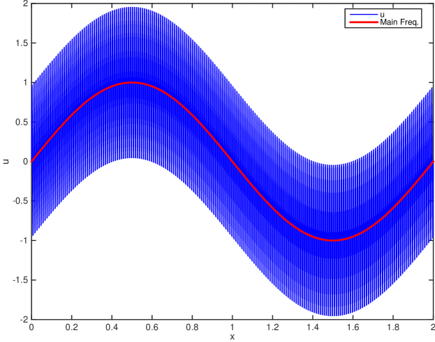
Then we discretize the interval with a step size of $h=\frac{2}{1000}$ (hence $1001$ sample points) and choose the filtering radius for the differential filter to be $\delta=6h$. To implement the Helmholtz filter, we begin with approximating the Laplacian operator with a center differencing scheme,

$$\Delta u\approx\Delta^{h}u=\frac{u(x-\Delta x)-2u(x)+u(x+\Delta x)}{(\Delta x)^{2}}.$$

and define our discrete operator, namely $A^{h}$ (the inverse operator to $G^{h}$) as

$$A^{h}\bar{u}=-\delta^{2}\Delta^{h}\bar{u}+\bar{u}\quad\text{and}\quad A^{h}G^{h}=I.$$

Our simulated data was obtained by filtering the true solution and adding $1\%$ random noise to the filtered data, that is, $\bar{u}=G^{h}u-\epsilon$ where $\|\epsilon\|=0.01*\|G^{h}u\|$ ($\epsilon$ is generated in Matlab using the command “randn”, and normalized to have $L^{2}$ norm of $1$). And for calculating the $L^{2}$ norm of a function $f$ over $[a,b]$, we use either the composite Trapezoidal rule or the composite Simpson’s rule. We select the regularization parameter $\alpha=0.1$ ($\alpha\leq 0.5$ to have a decreasing sequence for the noise free energy functional) for Mitlar. And we use the following guideline for finding the optimal stopping $J$:

1. At the $j^{th}$ iterate, except the initial iterate, we calculate $\left|\left|u_{j+1}-u_{j}\right|\right|$.

2. We then compare $\alpha$, the regularization parameter, to $\epsilon_{0}/\left|\left|u_{j+1}-u_{j}\right|\right|$.

3. According to (52): if $\alpha\geq\epsilon_{0}/\left|\left|u_{j+1}-u_{j}\right|\right|$, we proceed to next iterate; when $\alpha<\epsilon_{0}/\left|\left|u_{j+1}-u_{j}\right|\right|$, we stop the iteration.

The actual simulation which we did for this demonstration, on the other hand, will not stop once we find the stopping $J$; instead the optimal $J$ will be recorded.

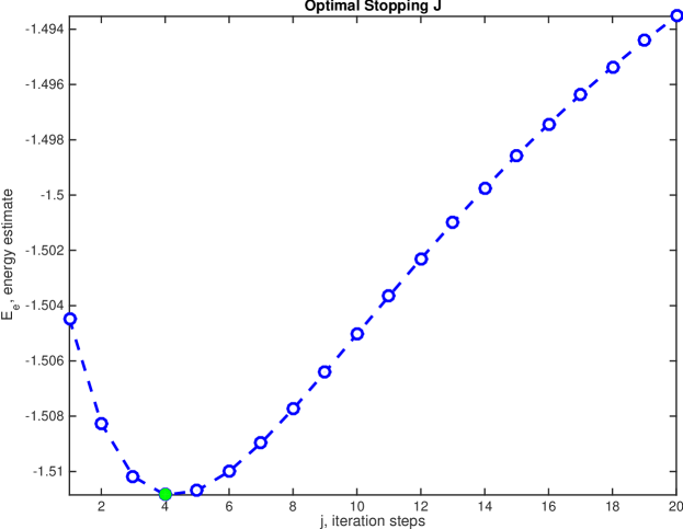
Figure 2 shows the noisy energy functional, $E_{\epsilon}$, calculated with the Mitlar approximation $u_{j}$’s when there is noise in the filtering process, i.e., $Gu=\bar{u}+\epsilon$. The calculated optimal stopping point (via Theorem 4.2) occurs after $J=4$ iteration steps and is shown as a green dot. The figure shows that the algorithm stops right where functional reaches its minimum and starts increasing again, hence avoiding the convergence to the noisy solution. However, because we do not have precise information of the noise (as it is always the case in real life applications), the algorithm will always try to stop before the energy functional reaches its minimum.

Figure 2. Noisy energy functional calculated for values of $J$ between $1$ and $20$. The stopping criterion forces us to stop after $4$ iteration steps (as shown with the green dot with white face color).

5.2. Comparison of four deconvolution algorithms

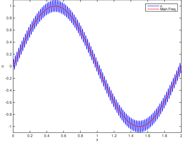
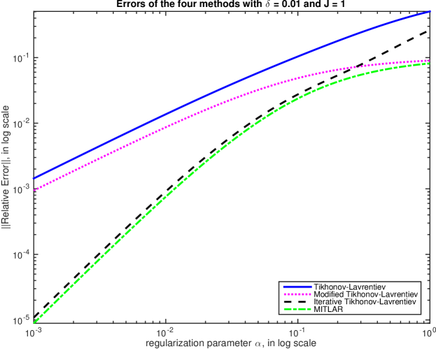
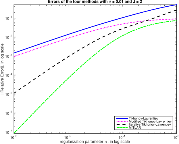
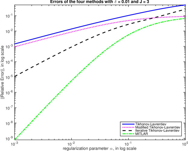
We check the efficiency of Algorithm 3.1 by comparing the relative error of a solution for a given parameter $\alpha$ to the relative errors found with Tikhonov-Lavrentiev, iterative Tikhonov-Lavrentiev, and Modified Tikhonov-Lavrentiev using the same $\alpha$. We implement the codes in MATLAB (version $R2014b$) with the following details: we start out with the original data as $u=sin(\pi x)+0.1sin(100\pi x)$, with $1001$ sample points taken over the interval $[0,2]$, see figure 3; hence the step size is $h=\frac{2}{1000}$. We set our filtering radius at $\delta=0.01$. We let the $\alpha$ vary from $1$ to $10^{-3}$ and calculate $1$, $2$, and $3$ steps for the two iterative methods. For an approximation $u_{appr.}$ to a desired solution $u$, the relative error, $Err_{rel}$, is defined as, $Err_{rel}=\left|\left|u-u_{appr.}\right|\right|/\left|\left|u\right|\right|$. The results are shown in Figures 4, 5, and 6 respectively. We see that the error in Mitlar is the lowest for any given $\alpha$; meanwhile as the number of iterates increases, the accuracy of Mitlar increases. We would like to point out that, for bigger $J$ (total iteration numbers), the difference between Mitlar and the other $3$ regularization methods widens for small $\alpha$.

Figure 3. $u=sin(\pi x)+0.1sin(100\pi x)$, use in performance comparison against Tikhonov-Lavrentiev, iterative Tikhonov-Lavrentiev, and Modified Tikhonov-Lavrentiev

Figure 4. Relative errors for the four algorithms over $\alpha=10^{-3}$ to $\alpha=1$ and $J=1$. Notice that the modified iterated Tikhonov-Lavrentiev plot has the lowest error over the entire range of regularization parameters. Notice that gap between Mitlar and iterative Tikhonov-Lavrentiev is small across the whole $\alpha$ range.

Figure 5. Relative errors for the four algorithms over $\alpha=10^{-3}$ to $\alpha=1$ and $J=2$. Notice that the modified iterated Tikhonov-Lavrentiev plot has the lowest error over the entire range of regularization parameters. Notice that gap between Mitlar and iterative Tikhonov-Lavrentiev increases as $\alpha\rightarrow 0$.

Figure 6. Relative errors for the four algorithms over $\alpha=10^{-3}$ to $\alpha=1$ and $J=3$. Notice that the modified iterated Tikhonov-Lavrentiev plot has the lowest error over the entire range of regularization parameters. Notice that gap between Mitlar and iterative Tikhonov-Lavrentiev further increases as $\alpha\rightarrow 0$.

5.3. Verification of convergence rates

We calculate the convergence rates of the family of Tikhonov-Lavrentiev regularization methods to verify the convergence rates predicted in Theorem 3.10. We take a true solution over the domain $[0,2]\times[0,2]$ of

$$u=\sin(\pi x)\sin(\pi y)+sin(20\pi x)sin(20\pi y).$$

see Figure 7.

Figure 7. $u=\sin(\pi x)\sin(\pi y)+sin(20\pi x)sin(20\pi y)$, used in the convergence rate analysis.

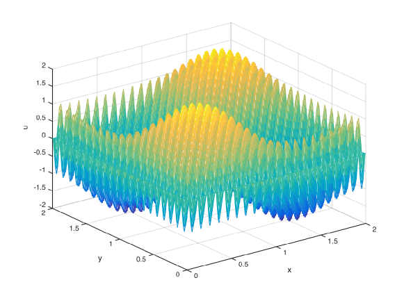
We discretize using the square command in FreeFEM++ [14] with $n$ intervals in each of $x$ and $y$ coordinates and use piecewise continuous linear polynomials. We use a filter radius of $\delta=0.1(\frac{2\pi}{n})^{1/4}=\mathcal{O}(h^{0.25})$ and regularization parameter $\alpha=0.1(\frac{2\pi}{n})^{1/2}=\mathcal{O}(h^{0.5})$. And the results are presented in the following tables.

Table 1. Convergence rates for modified Tikhonov-Lavrentiev (Mitlar with $J=0$). The convergence rates are approximating the theoretical value of $1$ in $H^{1}$ norm, since $\mathcal{O}(\alpha\delta^{2})=\mathcal{O}(h)$.

n	$L_{2}$ error	rate	$H_{1}$ error	rate
60	9.31514e-05		45.2992
120	1.23099e-05	2.9198	30.0506	0.5921
240	8.6617e-07	3.8290	15.9409	0.9147
480	6.22738e-08	3.7980	8.43094	0.9190
960	4.31597e-09	3.8509	4.38127	0.9443

Table 2. Convergence rates for Mitlar with $J=1$. The convergence rates are approximating the theoretical value of $2$ in $H^{1}$ norm, since $\mathcal{O}((\alpha\delta^{2})^{2})=\mathcal{O}(h^{2})$.

n	$L_{2}$ error	rate	$H_{1}$ error	rate
60	7.56535e-05		28.7953
120	4.44553e-07	7.4109	10.9148	1.3995
240	4.7906e-07	-0.1079	2.90149	1.9114
480	4.91109e-08	3.2861	0.802423	1.8544
960	3.87667e-09	3.6632	0.216175	1.8922

Table 3. Convergence rates for Tikhonov-Lavrentiev. The convergence rates are approximating the theoretical value of $0.5$ in $H^{1}$ norm, since $\mathcal{O}(\alpha)=\mathcal{O}(h^{0.5})$, superconvergence is obersved.

n	$L_{2}$ error	rate	$H_{1}$ error	rate
60	8.96747e-05		45.6474
120	1.17545e-05	2.9315	30.8419	0.5656
240	8.31362e-07	3.8216	16.8802	0.8696
480	6.03285e-08	3.7846	9.25259	0.8574
960	4.21634e-09	3.8388	5.02571	0.8805

Table 4. Convergence rates for iterated Tikhonov-Lavrentiev with $J=1$. The convergence rates are approximating the theoretical value of $1$ in $H^{1}$ norm, since $\mathcal{O}(\alpha^{2})=\mathcal{O}(h)$, superconvergence is observed.

n	$L_{2}$ error	rate	$H_{1}$ error	rate
60	7.50352e-05		29.1851
120	7.58837e-09	13.2715	11.4673	1.3477
240	4.29861e-07	-5.8239	3.25182	1.8182
480	4.58056e-08	3.2303	0.966347	1.7506
960	3.69301e-09	3.6327	0.284427	1.7645

6. Conclusion

We introduced a novel tool for solving some special types of inverse problems, that is, to deconvolve solutions filtered by a Helmholtz-type differential filter. We show that the noise free errors in using Mitlar are doubly asymptotic in $\alpha$ and $\delta$, that is $\mathcal{O}((\alpha\delta^{2})^{J+1})$. However, using the Tikhonov-Lavrentiev regularization or iterated Tikhonov-Lavrentiev regularization only results in the noise free errors depending solely on $\alpha$, which are $\mathcal{O}(\alpha)$ and $\mathcal{O}(\alpha^{J+1})$ respectively.

We also introduce a tool for calculating when to stop the iterations for our iterative algorithm. We show that continuing to iterate until the solution converges gives the unwanted and noisy solution. However, our stopping criterion guarantees that the iteration steps are getting closer to the original solution. The example chosen to illustrate the stopping criterion showed the exact optimal stopping, which is not always guaranteed due to insufficient knowledge of the noise. The actual implementation, on the other hand, will always try to stop before reaching the optimal number of iterations. And if we can incorporated more knowledge about the noise added into the model, then we would be able to get a more accurate bound on the optimal number of iterations.

Furthermore, we would like to point out that the analysis done in Mitlar can be applied to other filters whose transfer function behaves like the Pao filter for small wave lengths, due to the robustness of the Tikhonov-Lavrentiev regularization method.

References

- [1] A. K. Alekseev and I. M. Navon, The analysis of an ill-posed problem using multi-scale resolution and second-order adjoint techniques, C.M.A.M.E., 190 (2001), pp. 1937 – 1953.
- [2] A. B. Bakushinsky and M. Y. Kokurin, Iterative Methods for Approximate Solution of Inverse Problems, Kluwer, Dordrecht, the Netherlands, 2004.
- [3] L. Berselli, T. Iliescu, and W. J. Layton, Mathematics of Large Eddy Simulation of Turbulent Flows, Springer, Berlin, 2006.
- [4] M. Bertero and P. Boccacci, Introduction to Inverse Problems in Imaging, Institute of Physics Publishing Ltd., Bristol, UK, 1998.
- [5] S. Brenner and L. R. Scott, The Mathematical Theory of Finite Element Methods, Springer-Verlag, New York, 1994.
- [6] N. G. Deen, T. Solberg, and B. H. Hjertager, Large eddy simulation of the gas-liquid flow in a square cross-sectioned bubble column, Chemical Engineering Science, 56 (2001), pp. 6341 – 6349.
- [7] H. W. Engl, C. Flamm, P. Kügler, J. Lu, S. Müller, and P. Schuster, Inverse problems in systems biology, Inverse Problems, 25 (2009), pp. 1 – 51.
- [8] H. W. Engl, M. Hanke, and G. Neubauer, Regularization of Inverse Problems, Kluwer, Dordrecht, the Netherlands, 1996.
- [9] M. Germano, Differential filters for the large eddy numerical simulation of turbulent flows, Phys. Fluids, 29 (1986), pp. 1755–1757.
- [10] B. J. Geurts, Inverse modeling for large-eddy simulation, Phys. Fluids, 9 (1997), pp. 3585 – 3587.
- [11] M. Ghizaru, P. Charbonneau, and P. K. Smolarkiewicz, Magnetic cycles in global large-eddy simulations of solar convection, The Astrophysical Journal Letters, 715 (2010), pp. L133 – L137.
- [12] J. L. Guermond, J. T. Oden, and S. Prudhomme, Mathematical perspectives on large eddy simulation models for turbulent flows, Journal of Mathematical Fluid Mechanics, 6 (2004), pp. 194 – 248.
- [13] P. C. Hansen, Regularization tools: A matlab package for analysis and solution of discrete ill-posed problems, Numer. Algorithms, 6 (1994), pp. 1 – 35.
- [14] F. Hecht, New development in freefem++, J. Numer. Math., 20 (2012), pp. 251–265.
- [15] J. T. King and D. Chillingworth, Approximation of generalized inverses by iterated regularization, Numer. Functional Anal. and Optim., 1 (1979), pp. 499 – 513.
- [16] A. Labovschii and C. Trenchea, Approximate deconvolution models for magnetohydrodynamics, Numerical Functional Analysis and Optimization, 31 (2010), pp. 1362 – 1385.
- [17] M. M. Lavrentiev, Some Improperly Posed Problems of Mathematical Physics, Springer, New York, 1967.
- [18] W. J. Layton and R. Lewandowski, Residual stress of approximate deconvolution large eddy simulation models of turbulence, Journal of Turbulence, 7 (2006), pp. 1 – 21.
- [19] W. J. Layton and L. G. Rebholz, Approximate Deconvolution Models of Turbulence: Analysis, Phenomenology and Numerical Analysis, Springer-Verlag, Berlin, Heidelberg, 2012.
- [20] F. Liu and M. Z. Nashed, Convergence of regularized solutions of nonlinear ill-posed problems with monotone operators, in Partial Differential Equations and Applications, P. M. et al, ed., Dekker, New York, 1996, pp. 353 – 361.
- [21] C. C. Manica and S. K. Merdan, Convergence analysis of the finite element method for a fundamental model in turbulence, technical report, Mathematics Department, University of Pittsburgh, http://www.mathematics.pitt.edu/documents/0612.pdf, 2006.
- [22] C. C. Manica and I. Stanculescu, Numerical analysis of leray-tikhonov deconvolution models of fluid motion, Comput. Math. Appl., 60 (2010), pp. 1440 – 1456.
- [23] R. Mittal and P. Moin, Suitability of upwind-biased finite difference schemes for large-eddy simulation of turbulent flows, AIAA Journal, 35 (1997), pp. 1415 – 1417.
- [24] C.-H. Moeng, A large-eddy-simulation model for the study of planetary boundary-layer turbulence, J. Atmos. Sci., 41 (1984), pp. 2052 – 2062.
- [25] K. Nadaoka and H. Yagi, Shallow-water turbulence modeling and horizontal large-eddy computation of river flow, Journal of Hydraulic Engineering, 124 (1998), pp. 493 – 500.
- [26] F. Natterer, Error bounds for tikhonov regularization in hilbert scales, Appl. Anal., 18 (1984), pp. 262 – 270.
- [27] U. Piomelli, A. Scotti, and E. Balaras, Large-eddy simulations of turbulent flows, from desktop to supercomputer, in VECPAR 2000, LNCS 1981, P. et al., ed., Springer-Verlag, Berlin, Heidelberg, 2001, pp. 551 – 577.
- [28] T. Schuster, The Method of Approximate Inverse: Theory and Applications, Springer, Berlin, 2007.
- [29] K. B. Shah and J. H. Ferziger, A fluid mechanicians view of wind engineering: Large eddy simulation of flow past a cubic obstacle, Journal of Wind Engineering and Industrial Aerodynamics, 67 & 68 (1997), pp. 211 – 224.
- [30] S. Stolz, N. A. Adams, and L. Kleiser, The approximate deconvolution model for large-eddy simulations of compressible flows and its application to shock-turbulent-boundary-layer interaction, Physics of Fluids, 13 (2001), pp. 2985 – 3001.
- [31] A. N. Tikhonov and V. Y. Arsenin, Solutions of Ill-posed Problems, Halsted Press, New York, 1977.
- [32] , Methods of Solving Ill-posed Porlbmes in Hilbert Spaces, Nauka, Moskow, 1979.
- [33] G. M. Vainikko, Solution Methods for Linear Ill-posed Problems in Hilbert Spaces, Nauka, Moskow, 1982.
- [34] G. M. Vainikko and A. Y. Veretennikov, Iteration Procedures in Ill-posed Problems, Nauka, Moskow, 1982.
- [35] C. R. Vogel, Computational Methods for Inverse Problems, SIAM publications, Philadelphia, 2002.