Higgs alignment from extended supersymmetry

Abstract

We consider the effective type-II Two-Higgs doublet model originating from Dirac gaugino models with extended supersymmetry in the gauge sector, which is automatically aligned in the simplest realisations. We show that raising the scale at which the extended supersymmetry is manifest and including quantum corrections actually improves the alignment. Using an effective field theory approach including new threshold corrections and two-loop RGEs, plus two-loop corrections to the Higgs mass in the low-energy theory, we study the implications from the Higgs mass and other experimental constraints on the scale of superpartners. We contrast the results of the minimal Dirac gaugino model, where alignment is automatic, with the hMSSM and the MRSSM, where it is not, also providing an hMSSM-inspired analysis for the new models.

Higgs alignment from extended supersymmetry

Karim Benakli kbenakli@lpthe.jussieu.fr, Mark D. Goodsell goodsell@lpthe.jussieu.fr and Sophie L. Williamson swilliamson@lpthe.jussieu.fr

Laboratoire de Physique Théorique et Hautes Energies (LPTHE),
UMR 7589, Sorbonne Université et CNRS, 4 place Jussieu, 75252 Paris Cedex 05, France.

1 Introduction

In the absence of signals of strongly-coupled particles at the LHC, it has become important to study the possibility of new particles that couple to Standard Model (SM) states only via couplings of electroweak strength. The bounds on such particles are still relatively weak but with much luminosity to arrive there is still a substantial parameter space to explore, and such theories perhaps represent now the best chance for discoveries. Among such theories, one that has received significant and now increasing attention is the Two Higgs Doublet Model (THDM); see e.g. [1, 2, 3, 4] and references therein. It is important to ask the question: “does the Higgs sector just consist of one doublet?” because the answer will give profound information about nature. If there are indeed additional fundamental scalars that mix with the Higgs boson, then this dramatically worsens the Hierarchy problem and would necessitate a rethinking of our ideas of naturalness. On the other hand, such sectors naturally appear in the context of supersymmetry (SUSY) and it is conceivable that a second Higgs doublet could be the harbinger of a full SUSY theory.

However, the measurements of the Higgs boson’s couplings already place significant constraints on the amount of mixing that it can suffer. It is for this reason that there has been much interest in the idea of alignment in the Higgs sector, i.e. that the mass eigenstates align with the vacuum expectation value, because in this case the couplings would be exactly SM-like.

To quantify this, consider two Higgs doublets Φ1,Φ2subscriptΦ1subscriptΦ2\Phi_{1},\Phi_{2} which mix, and then rotate their neutral components as follows:

(Re(Φ10)Re(Φ20))=12(cβsβsβcβ)(v+h~H~)ResuperscriptsubscriptΦ10ResuperscriptsubscriptΦ2012subscript𝑐𝛽subscript𝑠𝛽subscript𝑠𝛽subscript𝑐𝛽𝑣~~𝐻\displaystyle\left(\begin{array}[]{c}\mathrm{Re}(\Phi_{1}^{0})\\ \mathrm{Re}(\Phi_{2}^{0})\end{array}\right)=\frac{1}{\sqrt{2}}\left(\begin{array}[]{cc}c_{\beta}&-s_{\beta}\\ s_{\beta}&c_{\beta}\end{array}\right)\left(\begin{array}[]{c}v+\tilde{h}\\ \tilde{H}\end{array}\right) (1.7)

where we shall throughout use the notation

cβcosβ,sβsinβ,tβtanβ.formulae-sequencesubscript𝑐𝛽𝛽formulae-sequencesubscript𝑠𝛽𝛽subscript𝑡𝛽𝛽c_{\beta}\equiv\cos\beta,\qquad s_{\beta}\equiv\sin\beta,\qquad t_{\beta}\equiv\tan\beta.

In this basis, we can write the mass matrix as

h2(Z1v2Z6v2Z6v2mA2+Z5v2),subscriptsuperscript2matrixsubscript𝑍1superscript𝑣2subscript𝑍6superscript𝑣2subscript𝑍6superscript𝑣2superscriptsubscript𝑚𝐴2subscript𝑍5superscript𝑣2\displaystyle\mathcal{M}^{2}_{h}\equiv\begin{pmatrix}Z_{1}v^{2}&Z_{6}v^{2}\\ Z_{6}v^{2}&m_{A}^{2}+Z_{5}v^{2}\end{pmatrix}, (1.8)

where the quantities Z1,Z5,Z6subscript𝑍1subscript𝑍5subscript𝑍6Z_{1},Z_{5},Z_{6} are functions of the quartic couplings and mixing angles only; we shall give explicit expressions for this relationship later, in equation (2.30). Clearly the mass eigenstates are only h~,H~~~𝐻\tilde{h},\tilde{H} if

Z6=0,subscript𝑍60Z_{6}=0,

and this is the condition for alignment, because the fields align with the electroweak vacuum expectation value. On the other hand, if Z60subscript𝑍60Z_{6}\neq 0, we must make a further rotation which is conventionally parameterised by an angle α𝛼\alpha as

(h~H~)=~~𝐻absent\displaystyle\left(\begin{array}[]{c}\tilde{h}\\ \tilde{H}\end{array}\right)= (sβαcβαcβαsβα)(hH)subscript𝑠𝛽𝛼subscript𝑐𝛽𝛼subscript𝑐𝛽𝛼subscript𝑠𝛽𝛼𝐻\displaystyle\left(\begin{array}[]{cc}s_{\beta-\alpha}&c_{\beta-\alpha}\\ c_{\beta-\alpha}&-s_{\beta-\alpha}\end{array}\right)\left(\begin{array}[]{c}h\\ H\end{array}\right) (1.15)

where now h,H𝐻h,H are the two mass eigenstates. We shall assume throughout that hh is the lightest eigenstate. In terms of the masses of the physical bosons mh,Hsubscript𝑚𝐻m_{h,H} this gives

Z6v2=subscript𝑍6superscript𝑣2absent\displaystyle Z_{6}v^{2}= sβαcβα(mh2mH2).subscript𝑠𝛽𝛼subscript𝑐𝛽𝛼superscriptsubscript𝑚2superscriptsubscript𝑚𝐻2\displaystyle s_{\beta-\alpha}c_{\beta-\alpha}(m_{h}^{2}-m_{H}^{2}). (1.16)

In both the type-I and type-II THDM, there is a Higgs eigenstate that couples to the up-type quarks, and we define this eigenstate to be Φ2subscriptΦ2\Phi_{2}. This means that the ratio of the hh coupling to all up-type quarks compared to the SM Higgs’ value is

κu=cosαsinβ,subscript𝜅𝑢𝛼𝛽\kappa_{u}=\frac{\cos\alpha}{\sin\beta},

while the ratio of the coupling to vector bosons to the SM value is also determined entirely by the mixing (neglecting loop effects from the rest of the extended Higgs sector):

κV=sin(βα).subscript𝜅𝑉𝛽𝛼\displaystyle\kappa_{V}=\sin(\beta-\alpha). (1.17)

However, there is a combined ATLAS+CMS bound [5] on the ratio of these:

λVuκVκu=10.12+0.13=11+1tβtβα.subscript𝜆𝑉𝑢subscript𝜅𝑉subscript𝜅𝑢subscriptsuperscript10.130.12111subscript𝑡𝛽subscript𝑡𝛽𝛼\displaystyle\lambda_{Vu}\equiv\frac{\kappa_{V}}{\kappa_{u}}=1^{+0.13}_{-0.12}=\frac{1}{1+\frac{1}{t_{\beta}t_{\beta-\alpha}}}. (1.18)

This is enough to constrain

tβtβα7.3|Z6||7.3tβ53+tβ2mH2mh2v2||0.5mH2mh2v2|,greater-than-or-equivalent-tosubscript𝑡𝛽subscript𝑡𝛽𝛼7.3subscript𝑍6less-than-or-similar-to7.3subscript𝑡𝛽53superscriptsubscript𝑡𝛽2superscriptsubscript𝑚𝐻2superscriptsubscript𝑚2superscript𝑣2less-than-or-similar-to0.5superscriptsubscript𝑚𝐻2superscriptsubscript𝑚2superscript𝑣2\displaystyle t_{\beta}t_{\beta-\alpha}\gtrsim 7.3\Rightarrow|Z_{6}|\lesssim\bigg{|}-\frac{7.3t_{\beta}}{53+t_{\beta}^{2}}\frac{m_{H}^{2}-m_{h}^{2}}{v^{2}}\bigg{|}\lesssim\bigg{|}-0.5\frac{m_{H}^{2}-m_{h}^{2}}{v^{2}}\bigg{|}, (1.19)

where the latter bound comes from the value tβ=7.3subscript𝑡𝛽7.3t_{\beta}=7.3, and the bound is much more stringent for large or small tβsubscript𝑡𝛽t_{\beta}. For mHsubscript𝑚𝐻m_{H} somewhat above mhsubscript𝑚m_{h} this is a rather weak constraint, only becoming relevant when the two states approach degeneracy. However, in the type-II THDM, there is another constraint from the ratio of the ratio of the neutral Higgs coupling to all down-type quarks compared to its SM value

κd=sinαcosβsubscript𝜅𝑑𝛼𝛽\kappa_{d}=-\frac{\sin\alpha}{\cos\beta}

via

λduκdκu=0.92±0.12=1tβtβα1+1tβtβαsubscript𝜆𝑑𝑢subscript𝜅𝑑subscript𝜅𝑢plus-or-minus0.920.121subscript𝑡𝛽subscript𝑡𝛽𝛼11subscript𝑡𝛽subscript𝑡𝛽𝛼\displaystyle\lambda_{du}\equiv\frac{\kappa_{d}}{\kappa_{u}}=0.92\pm 0.12=\frac{1-\frac{t_{\beta}}{t_{\beta-\alpha}}}{1+\frac{1}{t_{\beta}t_{\beta-\alpha}}} (1.20)

and, since from the previous constraint we know that the denominator is nearly equal to one, we have

0.04tβtβα0.2less-than-or-similar-to0.04subscript𝑡𝛽subscript𝑡𝛽𝛼less-than-or-similar-to0.2\displaystyle-0.04\lesssim\frac{t_{\beta}}{t_{\beta-\alpha}}\lesssim 0.2 (1.21)

which in turn implies tβαtβmuch-greater-thansubscript𝑡𝛽𝛼subscript𝑡𝛽t_{\beta-\alpha}\gg t_{\beta} and so sβαcβα1tβαsimilar-to-or-equalssubscript𝑠𝛽𝛼subscript𝑐𝛽𝛼1subscript𝑡𝛽𝛼s_{\beta-\alpha}c_{\beta-\alpha}\simeq\frac{1}{t_{\beta-\alpha}} and

0.04mH2mh2tβv2Z60.2mH2mh2tβv2.less-than-or-similar-to0.04superscriptsubscript𝑚𝐻2superscriptsubscript𝑚2subscript𝑡𝛽superscript𝑣2subscript𝑍6less-than-or-similar-to0.2superscriptsubscript𝑚𝐻2superscriptsubscript𝑚2subscript𝑡𝛽superscript𝑣2\displaystyle-0.04\frac{m_{H}^{2}-m_{h}^{2}}{t_{\beta}v^{2}}\lesssim Z_{6}\lesssim 0.2\frac{m_{H}^{2}-m_{h}^{2}}{t_{\beta}v^{2}}. (1.22)

This leads to a sensible constraint; for example, for mH=600subscript𝑚𝐻600m_{H}=600 GeV and tβ=5subscript𝑡𝛽5t_{\beta}=5 it leads to Z60.2less-than-or-similar-tosubscript𝑍60.2Z_{6}\lesssim 0.2. So we see that either we should take the mass mHsubscript𝑚𝐻m_{H} to be large, in which case we have decoupling, or we keep it light in order to possibly detect it at the LHC, in which case we need alignment without decoupling (see e.g. [6]). However, as we have seen this is non-trivial; as the LHC measurements become more precise, the constraints will tighten further, and it is in this spirit that it is important to consider models where the alignment is natural rather than ad hoc.

The problem for the different types of THDM is that alignment without decoupling is not generic when we choose the masses – or equivalently quartic couplings – from the bottom up. Hence it is logical to derive the couplings of the THDM from some higher-energy theory and look for cases where alignment arises naturally. For example, [7, 8, 9] proposed models which lead to a natural alignment condition, based on additional bosonic symmetries. Here, on the other hand, we shall show how alignment arises automatically in a class of supersymmetric models, in contrast to the MSSM or NMSSM [10], with the additional benefits of (greatly) increasing the naturalness of the model and being able to predict the scale of new superpartners. Moreover, we shall show that quantum corrections actually improve the alignment!

The class of models that we shall consider have a gauge sector which is enhanced to N=2𝑁2N=2 supersymmetry at a (potentially high) scale MN=2subscript𝑀𝑁2M_{N=2}. This fits into the framework of Dirac gaugino models, which have been well-studied in, for example, [11, 12, 13, 14, 15, 16, 17, 18, 19, 20, 21, 22, 23, 24, 25, 26, 27, 28, 29, 30, 31, 32, 33, 34, 35, 36, 37, 38, 39, 40, 41, 42, 43, 44, 45, 46, 47, 48, 49, 50, 51, 52, 53, 54, 55, 56, 57, 58, 59, 60, 61, 62, 63, 64, 65, 66, 67, 68, 69, 70, 71]. In particular, the idea of N=2𝑁2N=2 supersymmetry in the gauge sector only and the consequences for the Higgs sector were first explored in [16] and recently studied in [72, 73]. In general, though, this was either taken to be at the same scale as the other superpartners [73], or only a rough estimate of the main contribution of the chiral sector was included [16], while we shall show that increasing MN=2subscript𝑀𝑁2M_{N=2} improves alignment and increases naturalness!

In section 2 we will describe our theory and how it leads to natural alignment at tree level. In section 3 we will outline the effect of radiative corrections. In section 4 we perform a precision study of the model using an EFT approach to obtain the parameters at low energies, give predictions for the scale of new physics from the value of the Higgs mass, and explore the consequences for alignment. In section 5 we consider all of the relevant constraints on the model space, including the latest LHC search for decays to τ𝜏\tau pairs, bsγ𝑏𝑠𝛾b\rightarrow s\gamma searches and electroweak precision constraints, and show how this affects our model. In the appendix we give all of the one-loop threshold corrections for our model at the scale of supersymmetry. Finally, in section 6 we briefly consider the case of the MRSSM.

2 Alignment from extended supersymmety

2.1 The Higgs sector of Dirac gaugino models

2.1.1 The minimal model

To endow gauginos with a Dirac mass, at a minimum we need to add chiral fermions in the adjoint representation of each gauge group, which means adding adjoint chiral superfields: a singlet 𝐒𝐒\mathbf{S}, an SU(2)𝑆𝑈2SU(2) triplet 𝐓𝐓\mathbf{T}, and an SU(3)𝑆𝑈3SU(3) octet 𝐎𝐎\mathbf{O}. If we add just these fields, then we have the simplest Dirac-gaugino extension of the MSSM whose Higgs sector has been well studied [21, 26, 32, 44, 69]. However, we can then choose the superpotential according to the symmetries that we want to preserve. One motivation for the adjoint fields is as the additional degrees of freedom from an N=2𝑁2N=2 supersymmetric gauge multiplet, and then the Hu,Hdsubscript𝐻𝑢subscript𝐻𝑑H_{u},H_{d} fields become an N=2𝑁2N=2 hypermultiplet; in this work we shall assume that N=2𝑁2N=2 supersymmetry in the gauge/Higgs sector only is valid above some scale MN=2subscript𝑀𝑁2M_{N=2}. In this case, we can immediately write down the superpotential

WHiggs=μ𝕦𝕕+λS𝕊𝕦𝕕+2λT𝕕𝕋𝕦subscript𝑊Higgs𝜇subscript𝕦subscript𝕕subscript𝜆𝑆𝕊subscript𝕦subscript𝕕2subscript𝜆𝑇subscript𝕕𝕋subscript𝕦\displaystyle W_{\text{Higgs}}=\mu\,\mathbb{H_{u}}\cdot\mathbb{H_{d}}+\lambda_{S}\mathbb{S}\,\mathbb{H_{u}}\cdot\mathbb{H_{d}}+2\lambda_{T}\,\mathbb{H_{d}}\cdot\mathbb{T}\mathbb{H_{u}} (2.1)

which contains the only interactions compatible with N=2𝑁2N=2 SUSY and includes a central role for the R-symmetry. Indeed, under the R-symmetry of the N=1𝑁1N=1 theory the adjoint scalars must have zero charge, and this prevents couplings of the form S2,S3superscript𝑆2superscript𝑆3S^{2},S^{3} etc which would otherwise be permitted by the gauge symmetry. The condition of N=2𝑁2N=2 supersymmetry imposes

λS=12gY,λT=12g2formulae-sequencesubscript𝜆𝑆12subscript𝑔𝑌subscript𝜆𝑇12subscript𝑔2\displaystyle\lambda_{S}=\frac{1}{\sqrt{2}}g_{Y},\qquad\lambda_{T}=\frac{1}{\sqrt{2}}g_{2} (2.2)

(where gY,g2subscript𝑔𝑌subscript𝑔2g_{Y},g_{2} are the hypercharge and SU(2)𝑆𝑈2SU(2) gauge couplings) at the scale MN=2subscript𝑀𝑁2M_{N=2}, which we shall in general take to be greater than the N=1𝑁1N=1 SUSY scale.

We must also add supersymmetry-breaking terms, and these do not necessarily need to respect the same symmetries as supersymmetric terms. The most general choice that we can make for the Higgs and adjoint scalar sector for the standard soft terms is

standardsoft=mHu2|Hu|2+mHd2|Hd|2+Bμ(HuHd+h.c)+12Miλiλisubscriptstandardsoftsuperscriptsubscript𝑚subscript𝐻𝑢2superscriptsubscript𝐻𝑢2superscriptsubscript𝑚subscript𝐻𝑑2superscriptsubscript𝐻𝑑2subscript𝐵𝜇subscript𝐻𝑢subscript𝐻𝑑h.c12subscript𝑀𝑖subscript𝜆𝑖subscript𝜆𝑖\displaystyle\mathcal{L}_{\rm standard\ soft}=m_{H_{u}}^{2}|H_{u}|^{2}+m_{H_{d}}^{2}|H_{d}|^{2}+B_{\mu}(H_{u}\cdot H_{d}+\text{h.c})+\frac{1}{2}M_{i}\lambda_{i}\lambda_{i} (2.3)
+mS2|S|2+2mT2tr(TT)+12BS(S2+h.c)+BT(tr(TT)+h.c.)+mO2|O|2+BO(tr(OO)+h.c.)\displaystyle+m_{S}^{2}|S|^{2}+2m_{T}^{2}\text{tr}(T^{\dagger}T)+\frac{1}{2}B_{S}\left(S^{2}+h.c\right)+B_{T}\left(\text{tr}(TT)+h.c.\right)+m_{O}^{2}|O|^{2}+B_{O}\left(\text{tr}(OO)+h.c.\right)
+AS(SHuHd+h.c)+2AT(HdTHu+h.c)+Aκ3(S3+h.c.)+AST(Str(TT)+h.c)+ASO(Str(OO)+h.c),\displaystyle+A_{S}\left(SH_{u}\cdot H_{d}+h.c\right)+2A_{T}\left(H_{d}\cdot TH_{u}+h.c\right)+\frac{A_{\kappa}}{3}\left(S^{3}+h.c.\right)+A_{ST}\left(S\mathrm{tr}(TT)+h.c\right)+A_{SO}\left(S\mathrm{tr}(OO)+h.c\right),

where λi={λY,λ2,λ3}subscript𝜆𝑖subscript𝜆𝑌subscript𝜆2subscript𝜆3\lambda_{i}=\{\lambda_{Y},\lambda_{2},\lambda_{3}\} are the gauginos of hypercharge, SU(2)𝑆𝑈2SU(2) and SU(3)𝑆𝑈3SU(3) respectively, with Majorana masses MY,M2,M3subscript𝑀𝑌subscript𝑀2subscript𝑀3M_{Y},M_{2},M_{3}, and to these we add the supersoft operators mDiθαsubscript𝑚𝐷𝑖superscript𝜃𝛼m_{Di}\theta^{\alpha} for Dirac masses as

d2θ[2mDYθα𝕎1α𝕊+22mD2θαtr(𝕎2α𝕋)+22mD3θαtr(𝕎3α𝕆)]superscript𝑑2𝜃delimited-[]2subscript𝑚𝐷𝑌superscript𝜃𝛼subscript𝕎1𝛼𝕊22subscript𝑚𝐷2superscript𝜃𝛼trsubscript𝕎2𝛼𝕋22subscript𝑚𝐷3superscript𝜃𝛼trsubscript𝕎3𝛼𝕆\displaystyle\int d^{2}\theta\left[\sqrt{2}\,m_{DY}\theta^{\alpha}\mathbb{W}_{1\alpha}\mathbb{S}+2\sqrt{2}\,m_{D2}\theta^{\alpha}\text{tr}\left(\mathbb{W}_{2\alpha}\mathbb{T}\right)+2\sqrt{2}\,m_{D3}\theta^{\alpha}\text{tr}\left(\mathbb{W}_{3\alpha}\mathbb{O}\right)\!\right] (2.4)

where 𝕎iαsubscript𝕎𝑖𝛼\mathbb{W}_{i\alpha} are the supersymmetric gauge field strengths.

Since we are interested in Dirac gaugino masses and their attractive theoretical and phenomenological properties, we should expect that the terms that violate R-symmetry should be small: this includes the Majorana gaugino masses; AS,ATsubscript𝐴𝑆subscript𝐴𝑇A_{S},A_{T}; but also Bμsubscript𝐵𝜇B_{\mu}. However, we require that the R-symmetry is broken at some scale, since we believe that global symmetries cannot be exact; but also, in this model, the Higgs must carry R-charge and so the absence of an R-axion requires it. Indeed, the R-axion is essentially the Higgs pseudoscalar, whose mass is controlled by the Bμsubscript𝐵𝜇B_{\mu} term. We therefore, as in earlier works, take Bμsubscript𝐵𝜇B_{\mu} to have a small but non-zero value. We can also take motivation from models of gauge mediation of supersymmetry [20, 68], where the trilinears are all small, and we shall mostly neglect them in the following (although they do not significantly affect the analysis).

On the other hand, in gauge-mediated models the adjoint scalars are typically the heaviest states. Taking large mS,mT,mOsubscript𝑚𝑆subscript𝑚𝑇subscript𝑚𝑂m_{S},m_{T},m_{O} then motivates integrating them out of the light spectrum. Interestingly, since Bμsubscript𝐵𝜇B_{\mu} should remain small due to the approximate R-symmetry, if we were to tune the Higgs masses such that only one remains light, then we would have very large tanβ𝛽\tan\beta, and would have trouble obtaining the correct Yukawa couplings for the down-type quarks and leptons. This implies that a second Higgs should be taken to be somewhat light, and motivates studying the two-Higgs doublet limit of the model.

Finally, we note that this model does not have gauge-coupling unification. If we wish to naturally restore gauge coupling unification, we can add additional vector-like lepton fields, as was done in [55, 64]. Since they are vector-like, we could also allow them to be hypermultiplets of the N=2𝑁2N=2 at MN=2subscript𝑀𝑁2M_{N=2}, but their inclusion will little change the discussion in this paper so for sake of generality we shall neglect them.

2.1.2 The MRSSM

Another very popular realisation of Dirac gaugino models is the MRSSM [17, 54, 65, 66, 70]. In this model, we preserve an exact continuous R-symmetry by including some R-Higgs doublet superfields which couple to the Higgs bosons but do not obtain an expectation value, allowing the Higgs doublets Hu,Hdsubscript𝐻𝑢subscript𝐻𝑑H_{u},H_{d} to have zero R-charge. The Higgs superpotential becomes111We note the discrepancy of a factor of 222 for the triplet coupling terms compared to [54, 53], which arises due to a difference in definition of T𝑇T and the choice for the neutral components to take the same pre-factor as the singlet neutral components.

WHiggsMRSSMsuperscriptsubscript𝑊HiggsMRSSM\displaystyle W_{\text{Higgs}}^{\rm MRSSM} =\displaystyle= μu𝕦𝕦+μd𝕕𝕕+λSu𝕊𝕦𝕦+λSd𝕊𝕕𝕕subscript𝜇𝑢subscript𝕦subscript𝕦subscript𝜇𝑑subscript𝕕subscript𝕕subscript𝜆subscript𝑆𝑢𝕊subscript𝕦subscript𝕦subscript𝜆subscript𝑆𝑑𝕊subscript𝕕subscript𝕕\displaystyle\mu_{u}\,\mathbb{R_{u}}\cdot\mathbb{H_{u}}+\mu_{d}\,\mathbb{R_{d}}\cdot\mathbb{H_{d}}+\lambda_{S_{u}}\mathbb{S}\,\mathbb{R_{u}}\cdot\mathbb{H_{u}}+\lambda_{S_{d}}\mathbb{S}\,\mathbb{R_{d}}\cdot\mathbb{H_{d}} (2.5)
+2λTu𝕦𝕋𝕦+2λTd𝕕𝕋𝕕.2subscript𝜆subscript𝑇𝑢subscript𝕦𝕋subscript𝕦2subscript𝜆subscript𝑇𝑑subscript𝕕𝕋subscript𝕕\displaystyle+2\lambda_{T_{u}}\,\mathbb{R_{u}}\cdot\mathbb{T}\mathbb{H_{u}}+2\lambda_{T_{d}}\,\mathbb{R_{d}}\cdot\mathbb{T}\mathbb{H_{d}}\,.

If we then impose N=2𝑁2N=2 supersymmetry at some scale, we can treat (Ru,Hu)subscript𝑅𝑢subscript𝐻𝑢(R_{u},H_{u}) and (Rd,Hd)subscript𝑅𝑑subscript𝐻𝑑(R_{d},H_{d}) as hypermultiplets and then we would have

λSu=gY2,λSd=gY2,λTu=λTd=g22.,formulae-sequencesubscript𝜆subscript𝑆𝑢subscript𝑔𝑌2formulae-sequencesubscript𝜆subscript𝑆𝑑subscript𝑔𝑌2subscript𝜆subscript𝑇𝑢subscript𝜆subscript𝑇𝑑subscript𝑔22\displaystyle\lambda_{S_{u}}=\frac{g_{Y}}{\sqrt{2}},\qquad\lambda_{S_{d}}=-\frac{g_{Y}}{\sqrt{2}},\qquad\lambda_{T_{u}}=\lambda_{T_{d}}=\frac{g_{2}}{\sqrt{2}}., (2.6)

where the difference in sign is explained by the different charges of the hypermultiplets.222Equivalently the second hypermultiplet could be written (Hd,Rd)subscript𝐻𝑑subscript𝑅𝑑(H_{d},R_{d}) and then we would have λSd=gY/2,λTd=g2/2.formulae-sequencesubscript𝜆subscript𝑆𝑑subscript𝑔𝑌2subscript𝜆subscript𝑇𝑑subscript𝑔22\lambda_{S_{d}}=g_{Y}/\sqrt{2},\lambda_{T_{d}}=-g_{2}/\sqrt{2}.

R-symmetry then limits the possible soft-supersymmetry breaking terms to consist of only the supersoft operator, squark/slepton masses and

standardsoftMRSSM=mHu2|Hu|2+mHd2|Hd|2+Bμ(HuHd+h.c)+mRu2|Ru|2+mRd2|Rd|2superscriptsubscriptstandardsoftMRSSMsuperscriptsubscript𝑚subscript𝐻𝑢2superscriptsubscript𝐻𝑢2superscriptsubscript𝑚subscript𝐻𝑑2superscriptsubscript𝐻𝑑2subscript𝐵𝜇subscript𝐻𝑢subscript𝐻𝑑h.csuperscriptsubscript𝑚subscript𝑅𝑢2superscriptsubscript𝑅𝑢2superscriptsubscript𝑚subscript𝑅𝑑2superscriptsubscript𝑅𝑑2\displaystyle\mathcal{L}_{\rm standard\ soft}^{\rm MRSSM}=m_{H_{u}}^{2}|H_{u}|^{2}+m_{H_{d}}^{2}|H_{d}|^{2}+B_{\mu}(H_{u}\cdot H_{d}+\text{h.c})+m_{R_{u}}^{2}|R_{u}|^{2}+m_{R_{d}}^{2}|R_{d}|^{2} (2.7)
+mS2|S|2+2mT2tr(TT)+12BS(S2+h.c)+BT(tr(TT)+h.c.)+mO2|O|2+BO(tr(OO)+h.c.)\displaystyle+m_{S}^{2}|S|^{2}+2m_{T}^{2}\text{tr}(T^{\dagger}T)+\frac{1}{2}B_{S}\left(S^{2}+h.c\right)+B_{T}\left(\text{tr}(TT)+h.c.\right)+m_{O}^{2}|O|^{2}+B_{O}\left(\text{tr}(OO)+h.c.\right)
+AS(SHuHd+h.c)+2AT(HdTHu+h.c)+Aκ3(S3+h.c.)+AST(Str(TT)+h.c)+ASO(Str(OO)+h.c).\displaystyle+A_{S}\left(SH_{u}\cdot H_{d}+h.c\right)+2A_{T}\left(H_{d}\cdot TH_{u}+h.c\right)+\frac{A_{\kappa}}{3}\left(S^{3}+h.c.\right)+A_{ST}\left(S\mathrm{tr}(TT)+h.c\right)+A_{SO}\left(S\mathrm{tr}(OO)+h.c\right).

The terms on the last line are usually neglected, but there is no symmetry that forbids them (even if we expect them to be small in e.g. gauge mediation models).

2.2 Two-Higgs doublet model limit

The Higgs sectors of the models in the previous subsection have been comprehensively studied. However, here we wish to map them onto the two Higgs doublet model once the adjoint scalars have been integrated out. The standard parametrisation of the Two-Higgs doublet model is

VEWsubscript𝑉𝐸𝑊\displaystyle V_{EW} =\displaystyle= m112Φ1Φ1+m222Φ2Φ2[m122Φ1Φ2+h.c]+12λ1(Φ1Φ1)2+12λ2(Φ2Φ2)2superscriptsubscript𝑚112superscriptsubscriptΦ1subscriptΦ1superscriptsubscript𝑚222superscriptsubscriptΦ2subscriptΦ2delimited-[]superscriptsubscript𝑚122superscriptsubscriptΦ1subscriptΦ2h.c12subscript𝜆1superscriptsuperscriptsubscriptΦ1subscriptΦ1212subscript𝜆2superscriptsuperscriptsubscriptΦ2subscriptΦ22\displaystyle m_{11}^{2}\Phi_{1}^{\dagger}\Phi_{1}+m_{22}^{2}\Phi_{2}^{\dagger}\Phi_{2}-[m_{12}^{2}\Phi_{1}^{\dagger}\Phi_{2}+\text{h.c}]+\frac{1}{2}\lambda_{1}(\Phi_{1}^{\dagger}\Phi_{1})^{2}+\frac{1}{2}\lambda_{2}(\Phi_{2}^{\dagger}\Phi_{2})^{2} (2.8)
+λ3(Φ1Φ1)(Φ2Φ2)+λ4(Φ1Φ2)(Φ2Φ1)subscript𝜆3superscriptsubscriptΦ1subscriptΦ1superscriptsubscriptΦ2subscriptΦ2subscript𝜆4superscriptsubscriptΦ1subscriptΦ2superscriptsubscriptΦ2subscriptΦ1\displaystyle+\lambda_{3}(\Phi_{1}^{\dagger}\Phi_{1})(\Phi_{2}^{\dagger}\Phi_{2})+\lambda_{4}(\Phi_{1}^{\dagger}\Phi_{2})(\Phi_{2}^{\dagger}\Phi_{1})
+[12λ5(Φ1Φ2)2+[λ6(Φ1Φ1)+λ7(Φ2Φ2)]Φ1Φ2+h.c],delimited-[]12subscript𝜆5superscriptsuperscriptsubscriptΦ1subscriptΦ22delimited-[]subscript𝜆6superscriptsubscriptΦ1subscriptΦ1subscript𝜆7superscriptsubscriptΦ2subscriptΦ2superscriptsubscriptΦ1subscriptΦ2h.c\displaystyle+\left[\frac{1}{2}\lambda_{5}(\Phi_{1}^{\dagger}\Phi_{2})^{2}+[\lambda_{6}(\Phi_{1}^{\dagger}\Phi_{1})+\lambda_{7}(\Phi_{2}^{\dagger}\Phi_{2})]\Phi_{1}^{\dagger}\Phi_{2}+\text{h.c}\right]\,,\,

To map our supersymmetric model onto this, we choose to make the identification

Φ2=Hu,Φ1i=ϵij(Hdj)(Hd0Hd)=(Φ10(Φ1+))formulae-sequencesubscriptΦ2subscript𝐻𝑢superscriptsubscriptΦ1𝑖subscriptitalic-ϵ𝑖𝑗superscriptsuperscriptsubscript𝐻𝑑𝑗superscriptsubscript𝐻𝑑0superscriptsubscript𝐻𝑑superscriptsubscriptΦ10superscriptsuperscriptsubscriptΦ1\displaystyle\Phi_{2}=H_{u},\qquad\Phi_{1}^{i}=-\epsilon_{ij}(H_{d}^{j})^{*}\leftrightarrow\left(\begin{array}[]{c}H_{d}^{0}\\ H_{d}^{-}\end{array}\right)=\left(\begin{array}[]{c}\Phi_{1}^{0}\\ -(\Phi_{1}^{+})^{*}\end{array}\right) (2.13)

from which we can write down

m112superscriptsubscript𝑚112\displaystyle m_{11}^{2} =\displaystyle= mHd2+μ2,m222=mHu2+μ2,m122=Bμ.formulae-sequencesuperscriptsubscript𝑚subscript𝐻𝑑2superscript𝜇2superscriptsubscript𝑚222superscriptsubscript𝑚subscript𝐻𝑢2superscript𝜇2superscriptsubscript𝑚122subscript𝐵𝜇\displaystyle m_{H_{d}}^{2}+\mu^{2},\qquad m_{22}^{2}=m_{H_{u}}^{2}+\mu^{2},\qquad m_{12}^{2}=B_{\mu}. (2.14)

The parameters λisubscript𝜆𝑖\lambda_{i} were given at tree-level and with some loop corrections in [21, 44] in the limit of neglecting μ𝜇\mu and mDY,mD2subscript𝑚𝐷𝑌subscript𝑚𝐷2m_{DY},m_{D2}. However, when we integrate out the adjoint scalars and retain these terms, there are corrections due to the presence of trilinear couplings; setting the parameters AS,ATsubscript𝐴𝑆subscript𝐴𝑇A_{S},A_{T} to zero, we find for the minimal model:

λ1=subscript𝜆1absent\displaystyle\lambda_{1}= 14(g22+gY2)(gYmDY2λSμ)2mSR2(gmD2+2λTμ)2mTP214superscriptsubscript𝑔22superscriptsubscript𝑔𝑌2superscriptsubscript𝑔𝑌subscript𝑚𝐷𝑌2subscript𝜆𝑆𝜇2superscriptsubscript𝑚𝑆𝑅2superscript𝑔subscript𝑚𝐷22subscript𝜆𝑇𝜇2superscriptsubscript𝑚𝑇𝑃2\displaystyle\frac{1}{4}(g_{2}^{2}+g_{Y}^{2})-\frac{\left(g_{Y}m_{DY}-\sqrt{2}\lambda_{S}\mu\right)^{2}}{m_{SR}^{2}}-\frac{\left(gm_{D2}+\sqrt{2}\lambda_{T}\mu\right)^{2}}{m_{TP}^{2}}
λ2=subscript𝜆2absent\displaystyle\lambda_{2}= 14(g22+gY2)(gYmDY+2λSμ)2mSR2(gmD22λTμ)2mTP214superscriptsubscript𝑔22superscriptsubscript𝑔𝑌2superscriptsubscript𝑔𝑌subscript𝑚𝐷𝑌2subscript𝜆𝑆𝜇2superscriptsubscript𝑚𝑆𝑅2superscript𝑔subscript𝑚𝐷22subscript𝜆𝑇𝜇2superscriptsubscript𝑚𝑇𝑃2\displaystyle\frac{1}{4}(g_{2}^{2}+g_{Y}^{2})-\frac{\left(g_{Y}m_{DY}+\sqrt{2}\lambda_{S}\mu\right)^{2}}{m_{SR}^{2}}-\frac{\left(gm_{D2}-\sqrt{2}\lambda_{T}\mu\right)^{2}}{m_{TP}^{2}}
λ3=subscript𝜆3absent\displaystyle\lambda_{3}= 14(g22gY2)+2λT2+gY2mDY22λS2μ2mSR2g2mD222λT2μ2mTP214superscriptsubscript𝑔22superscriptsubscript𝑔𝑌22superscriptsubscript𝜆𝑇2superscriptsubscript𝑔𝑌2superscriptsubscript𝑚𝐷𝑌22superscriptsubscript𝜆𝑆2superscript𝜇2superscriptsubscript𝑚𝑆𝑅2superscript𝑔2superscriptsubscript𝑚𝐷222superscriptsubscript𝜆𝑇2superscript𝜇2superscriptsubscript𝑚𝑇𝑃2\displaystyle\frac{1}{4}(g_{2}^{2}-g_{Y}^{2})+2\lambda_{T}^{2}+\frac{g_{Y}^{2}m_{DY}^{2}-2\lambda_{S}^{2}\mu^{2}}{m_{SR}^{2}}-\frac{g^{2}m_{D2}^{2}-2\lambda_{T}^{2}\mu^{2}}{m_{TP}^{2}}
λ4=subscript𝜆4absent\displaystyle\lambda_{4}= 12g22+λS2λT2+2g22mD224λT2μ2mTP2,12superscriptsubscript𝑔22superscriptsubscript𝜆𝑆2superscriptsubscript𝜆𝑇22superscriptsubscript𝑔22superscriptsubscript𝑚𝐷224superscriptsubscript𝜆𝑇2superscript𝜇2superscriptsubscript𝑚𝑇𝑃2\displaystyle-\frac{1}{2}g_{2}^{2}+\lambda_{S}^{2}-\lambda_{T}^{2}+\frac{2g_{2}^{2}m_{D2}^{2}-4\lambda_{T}^{2}\mu^{2}}{m_{TP}^{2}}\,,
λ5=subscript𝜆5absent\displaystyle\lambda_{5}= λ6=λ7=0.subscript𝜆6subscript𝜆70\displaystyle\lambda_{6}=\lambda_{7}=0. (2.15)

Here we have defined

mSR2superscriptsubscript𝑚𝑆𝑅2absent\displaystyle m_{SR}^{2}\equiv mS2+BS+4mDY2,mTP2mT2+BT+4mD22.superscriptsubscript𝑚𝑆2subscript𝐵𝑆4superscriptsubscript𝑚𝐷𝑌2superscriptsubscript𝑚𝑇𝑃2superscriptsubscript𝑚𝑇2subscript𝐵𝑇4superscriptsubscript𝑚𝐷22\displaystyle m_{S}^{2}+B_{S}+4m_{DY}^{2},\qquad m_{TP}^{2}\equiv m_{T}^{2}+B_{T}+4m_{D2}^{2}. (2.16)

In fact, the terms suppressed by mSR,mTPsubscript𝑚𝑆𝑅subscript𝑚𝑇𝑃m_{SR},m_{TP} all have the effect of suppressing the Higgs quartic coupling: in the limit of large Dirac gaugino masses so that we can neglect mS2,BS,mT2,BTsuperscriptsubscript𝑚𝑆2subscript𝐵𝑆superscriptsubscript𝑚𝑇2subscript𝐵𝑇m_{S}^{2},B_{S},m_{T}^{2},B_{T} we find

λ1,λ20,λ32λT2,λ4λS2λT2.formulae-sequencesubscript𝜆1subscript𝜆20formulae-sequencesubscript𝜆32superscriptsubscript𝜆𝑇2subscript𝜆4superscriptsubscript𝜆𝑆2superscriptsubscript𝜆𝑇2\displaystyle\lambda_{1},\lambda_{2}\rightarrow 0,\qquad\lambda_{3}\rightarrow 2\lambda_{T}^{2},\qquad\lambda_{4}\rightarrow\lambda_{S}^{2}-\lambda_{T}^{2}. (2.17)

This simply corresponds to the well-known fact (see e.g. [14]) that the adjoint scalars eliminate the D-term potential of the Higgs, because they couple via the D-term. Writing ϕisubscriptitalic-ϕ𝑖\phi_{i} for (anti)fundamental scalars and ΣΣ\Sigma for adjoint scalars, we have

absent\displaystyle\mathcal{L}\supset 2mDΣΣaDa+gDaϕiTaϕiVD=12(2mDΣΣa+gϕiTaϕi)22subscript𝑚𝐷ΣsuperscriptΣ𝑎superscript𝐷𝑎𝑔superscript𝐷𝑎superscriptsubscriptitalic-ϕ𝑖superscript𝑇𝑎subscriptitalic-ϕ𝑖subscript𝑉𝐷12superscript2subscript𝑚𝐷ΣsuperscriptΣ𝑎𝑔superscriptsubscriptitalic-ϕ𝑖superscript𝑇𝑎subscriptitalic-ϕ𝑖2\displaystyle\sqrt{2}m_{D\Sigma}\Sigma^{a}D^{a}+gD^{a}\phi_{i}^{*}T^{a}\phi_{i}\rightarrow V_{D}=\frac{1}{2}\left(\sqrt{2}m_{D\Sigma}\Sigma^{a}+g\phi_{i}^{*}T^{a}\phi_{i}\right)^{2} (2.18)

where Tasuperscript𝑇𝑎T^{a} are the generators of the gauge group with coupling g𝑔g, and we see that the above will always be zero when we integrate out ΣΣ\Sigma.

For the MRSSM, for simplicity again neglecting AS,ATsubscript𝐴𝑆subscript𝐴𝑇A_{S},A_{T} – for completeness we give the full corrections in appendix D.1 – we find

λ1MRSSM=superscriptsubscript𝜆1MRSSMabsent\displaystyle\lambda_{1}^{\rm MRSSM}= 14(g22+gY2)(gYmDY2λSdμd)2mSR2(g2mD2+2λTdμd)2mTP214superscriptsubscript𝑔22superscriptsubscript𝑔𝑌2superscriptsubscript𝑔𝑌subscript𝑚𝐷𝑌2subscript𝜆subscript𝑆𝑑subscript𝜇𝑑2superscriptsubscript𝑚𝑆𝑅2superscriptsubscript𝑔2subscript𝑚𝐷22subscript𝜆subscript𝑇𝑑subscript𝜇𝑑2superscriptsubscript𝑚𝑇𝑃2\displaystyle\frac{1}{4}(g_{2}^{2}+g_{Y}^{2})-\frac{(g_{Y}m_{DY}-\sqrt{2}\lambda_{S_{d}}\mu_{d})^{2}}{m_{SR}^{2}}-\frac{(g_{2}m_{D2}+\sqrt{2}\lambda_{T_{d}}\mu_{d})^{2}}{m_{TP}^{2}}
λ2MRSSM=superscriptsubscript𝜆2MRSSMabsent\displaystyle\lambda_{2}^{\rm MRSSM}= 14(g22+gY2)(gYmDY+2λSuμu)2mSR2(g2mD2+2λTuμu)2mTP214superscriptsubscript𝑔22superscriptsubscript𝑔𝑌2superscriptsubscript𝑔𝑌subscript𝑚𝐷𝑌2subscript𝜆subscript𝑆𝑢subscript𝜇𝑢2superscriptsubscript𝑚𝑆𝑅2superscriptsubscript𝑔2subscript𝑚𝐷22subscript𝜆subscript𝑇𝑢subscript𝜇𝑢2superscriptsubscript𝑚𝑇𝑃2\displaystyle\frac{1}{4}(g_{2}^{2}+g_{Y}^{2})-\frac{(g_{Y}m_{DY}+\sqrt{2}\lambda_{S_{u}}\mu_{u})^{2}}{m_{SR}^{2}}-\frac{(g_{2}m_{D2}+\sqrt{2}\lambda_{T_{u}}\mu_{u})^{2}}{m_{TP}^{2}}
λ3MRSSM=superscriptsubscript𝜆3MRSSMabsent\displaystyle\lambda_{3}^{\rm MRSSM}= 14(g22gY2)14superscriptsubscript𝑔22superscriptsubscript𝑔𝑌2\displaystyle\frac{1}{4}(g_{2}^{2}-g_{Y}^{2})
+(gYmDY2λSdμd)(gYmDY+2λSuμu)mSR2(g2mD2+2λTdμd)(g2mD2+2λTuμu)mTP2subscript𝑔𝑌subscript𝑚𝐷𝑌2subscript𝜆subscript𝑆𝑑subscript𝜇𝑑subscript𝑔𝑌subscript𝑚𝐷𝑌2subscript𝜆subscript𝑆𝑢subscript𝜇𝑢superscriptsubscript𝑚𝑆𝑅2subscript𝑔2subscript𝑚𝐷22subscript𝜆subscript𝑇𝑑subscript𝜇𝑑subscript𝑔2subscript𝑚𝐷22subscript𝜆subscript𝑇𝑢subscript𝜇𝑢superscriptsubscript𝑚𝑇𝑃2\displaystyle+\frac{(g_{Y}m_{DY}-\sqrt{2}\lambda_{S_{d}}\mu_{d})(g_{Y}m_{DY}+\sqrt{2}\lambda_{S_{u}}\mu_{u})}{m_{SR}^{2}}-\frac{(g_{2}m_{D2}+\sqrt{2}\lambda_{T_{d}}\mu_{d})(g_{2}m_{D2}+\sqrt{2}\lambda_{T_{u}}\mu_{u})}{m_{TP}^{2}}
λ4MRSSM=superscriptsubscript𝜆4MRSSMabsent\displaystyle\lambda_{4}^{\rm MRSSM}= 12g22+2(g2mD2+2λTdμd)(g2mD2+2λTuμu)mTP212superscriptsubscript𝑔222subscript𝑔2subscript𝑚𝐷22subscript𝜆subscript𝑇𝑑subscript𝜇𝑑subscript𝑔2subscript𝑚𝐷22subscript𝜆subscript𝑇𝑢subscript𝜇𝑢superscriptsubscript𝑚𝑇𝑃2\displaystyle-\frac{1}{2}g_{2}^{2}+2\frac{(g_{2}m_{D2}+\sqrt{2}\lambda_{T_{d}}\mu_{d})(g_{2}m_{D2}+\sqrt{2}\lambda_{T_{u}}\mu_{u})}{m_{TP}^{2}}
λ5MRSSM=superscriptsubscript𝜆5MRSSMabsent\displaystyle\lambda_{5}^{\rm MRSSM}= λ6MRSSM=λ7MRSSM=0.superscriptsubscript𝜆6MRSSMsuperscriptsubscript𝜆7MRSSM0\displaystyle\lambda_{6}^{\rm MRSSM}=\lambda_{7}^{\rm MRSSM}=0. (2.19)

In this case, the supersoft limit is even worse, because in that limit all of the λisubscript𝜆𝑖\lambda_{i} vanish. However, even with the additions of λSsubscript𝜆𝑆\lambda_{S} and λTsubscript𝜆𝑇\lambda_{T} in the minimal model, the potential is not stable in this limit – for example if Hdsubscript𝐻𝑑H_{d} or Husubscript𝐻𝑢H_{u} are set to zero the quartic terms vanish – and so we would require loop corrections to prevent runaway vacua. An investigation of whether this is even viable is beyond the scope of this paper: instead, since we do not want to substantially reduce the Higgs quartic coupling at low scales we shall consider instead that |mDY|mS,|mD2|mTformulae-sequencemuch-less-thansubscript𝑚𝐷𝑌subscript𝑚𝑆much-less-thansubscript𝑚𝐷2subscript𝑚𝑇|m_{DY}|\ll m_{S},|m_{D2}|\ll m_{T}. As is also well known (see e.g. [32, 44]) and we shall later discuss, this limit is also imposed on us by electroweak precision tests. In this limit we have instead at tree-level

λ1,λ214(g22+gY2),λ314(g22gY2)+2λT2,λ412gY2+λS2λT2,formulae-sequencesubscript𝜆1subscript𝜆214superscriptsubscript𝑔22superscriptsubscript𝑔𝑌2formulae-sequencesubscript𝜆314superscriptsubscript𝑔22superscriptsubscript𝑔𝑌22superscriptsubscript𝜆𝑇2subscript𝜆412superscriptsubscript𝑔𝑌2superscriptsubscript𝜆𝑆2superscriptsubscript𝜆𝑇2\displaystyle\lambda_{1},\lambda_{2}\rightarrow\frac{1}{4}(g_{2}^{2}+g_{Y}^{2}),\qquad\lambda_{3}\rightarrow\frac{1}{4}(g_{2}^{2}-g_{Y}^{2})+2\lambda_{T}^{2},\qquad\lambda_{4}\rightarrow-\frac{1}{2}g_{Y}^{2}+\lambda_{S}^{2}-\lambda_{T}^{2}, (2.20)

and λiMRSSMλiMSSMsuperscriptsubscript𝜆𝑖MRSSMsuperscriptsubscript𝜆𝑖𝑀𝑆𝑆𝑀\lambda_{i}^{\rm MRSSM}\rightarrow\lambda_{i}^{MSSM}:

λ1MSSM,λ2MSSM14(g22+gY2),λ3MSSM14(g22gY2),λ4MSSM12gY2.formulae-sequencesuperscriptsubscript𝜆1MSSMsuperscriptsubscript𝜆2MSSM14superscriptsubscript𝑔22superscriptsubscript𝑔𝑌2formulae-sequencesuperscriptsubscript𝜆3MSSM14superscriptsubscript𝑔22superscriptsubscript𝑔𝑌2superscriptsubscript𝜆4MSSM12superscriptsubscript𝑔𝑌2\displaystyle\lambda_{1}^{\rm MSSM},\lambda_{2}^{\rm MSSM}\rightarrow\frac{1}{4}(g_{2}^{2}+g_{Y}^{2}),\qquad\lambda_{3}^{\rm MSSM}\rightarrow\frac{1}{4}(g_{2}^{2}-g_{Y}^{2}),\qquad\lambda_{4}^{\rm MSSM}\rightarrow-\frac{1}{2}g_{Y}^{2}. (2.21)

Hence for the rest of the paper we shall consider our low-energy theory to be a type-II two Higgs doublet model with an additional (Dirac) bino and wino (the gluino must remain heavy due to LHC constraints – currently of the order of 222 TeV). We shall fix the boundary conditions at high energies and find some interesting conclusions.

2.3 Tree-level alignment

In [16, 73] the Higgs sector of Dirac gaugino models was investigated in the limit that the couplings λS,λTsubscript𝜆𝑆subscript𝜆𝑇\lambda_{S},\lambda_{T} took their N=2𝑁2N=2 supersymmetric values at the low energy scale. However, they also pointed out that alignment in the Higgs sector would be broken by quantum corrections to the (2,2)22(2,2) element of the Higgs mass matrix. In this section we shall consider just the potential at tree-level, and in section 4 consider loop corrections, contrasting our results with theirs.

To begin with, the mass-matrices for the CP-even neutral scalars in the two-Higgs doublet model can be parametrised in the alignment basis where

(Re(Φ1)Re(Φ2))=12(cβsβsβcβ)(v+hH)ResubscriptΦ1ResubscriptΦ212subscript𝑐𝛽subscript𝑠𝛽subscript𝑠𝛽subscript𝑐𝛽𝑣𝐻\displaystyle\left(\begin{array}[]{c}\mathrm{Re}(\Phi_{1})\\ \mathrm{Re}(\Phi_{2})\end{array}\right)=\frac{1}{\sqrt{2}}\left(\begin{array}[]{cc}c_{\beta}&-s_{\beta}\\ s_{\beta}&c_{\beta}\end{array}\right)\left(\begin{array}[]{c}v+h\\ H\end{array}\right) (2.28)

is (see e.g. [1, 2, 3])

h2=(Z1v2Z6v2Z6v2mA2+Z5v2),subscriptsuperscript2matrixsubscript𝑍1superscript𝑣2subscript𝑍6superscript𝑣2subscript𝑍6superscript𝑣2superscriptsubscript𝑚𝐴2subscript𝑍5superscript𝑣2\displaystyle\mathcal{M}^{2}_{h}=\begin{pmatrix}Z_{1}v^{2}&Z_{6}v^{2}\\ Z_{6}v^{2}&m_{A}^{2}+Z_{5}v^{2}\end{pmatrix}\,, (2.29)

where, using λ345λ3+λ4+λ5subscript𝜆345subscript𝜆3subscript𝜆4subscript𝜆5\lambda_{345}\equiv\lambda_{3}+\lambda_{4}+\lambda_{5} we have

Z1subscript𝑍1absent\displaystyle Z_{1}\equiv λ1cβ4+λ2sβ4+12λ345s2β2,Z514s2β2[λ1+λ22λ345]+λ5subscript𝜆1superscriptsubscript𝑐𝛽4subscript𝜆2superscriptsubscript𝑠𝛽412subscript𝜆345superscriptsubscript𝑠2𝛽2subscript𝑍514superscriptsubscript𝑠2𝛽2delimited-[]subscript𝜆1subscript𝜆22subscript𝜆345subscript𝜆5\displaystyle\lambda_{1}c_{\beta}^{4}+\lambda_{2}s_{\beta}^{4}+\frac{1}{2}\lambda_{345}s_{2\beta}^{2},\qquad Z_{5}\equiv\frac{1}{4}s_{2\beta}^{2}\left[\lambda_{1}+\lambda_{2}-2\lambda_{345}\right]+\lambda_{5}
Z6subscript𝑍6absent\displaystyle Z_{6}\equiv 12s2β[λ1cβ2λ2sβ2λ345c2β].12subscript𝑠2𝛽delimited-[]subscript𝜆1superscriptsubscript𝑐𝛽2subscript𝜆2superscriptsubscript𝑠𝛽2subscript𝜆345subscript𝑐2𝛽\displaystyle-\frac{1}{2}s_{2\beta}\left[\lambda_{1}c_{\beta}^{2}-\lambda_{2}s_{\beta}^{2}-\lambda_{345}c_{2\beta}\right]. (2.30)

The parameter mAsubscript𝑚𝐴m_{A} is the pseudoscalar mass, given by

mA2=superscriptsubscript𝑚𝐴2absent\displaystyle m_{A}^{2}= m122sβcβλ5v2,superscriptsubscript𝑚122subscript𝑠𝛽subscript𝑐𝛽subscript𝜆5superscript𝑣2\displaystyle-\frac{m_{12}^{2}}{s_{\beta}c_{\beta}}-\lambda_{5}v^{2}, (2.31)

while the charged Higgs mass is

mH+2=superscriptsubscript𝑚superscript𝐻2absent\displaystyle m_{H^{+}}^{2}= 12(λ5λ4)v2+mA2.12subscript𝜆5subscript𝜆4superscript𝑣2superscriptsubscript𝑚𝐴2\displaystyle\frac{1}{2}(\lambda_{5}-\lambda_{4})v^{2}+m_{A}^{2}. (2.32)

The neutral Higgs masses are

mH,h2superscriptsubscript𝑚𝐻2\displaystyle m_{H,h}^{2} =\displaystyle= 12[mA2+(Z1+Z5)v2±(mA2+(Z5Z1)v2)2+4Z62v4].12delimited-[]plus-or-minussuperscriptsubscript𝑚𝐴2subscript𝑍1subscript𝑍5superscript𝑣2superscriptsuperscriptsubscript𝑚𝐴2subscript𝑍5subscript𝑍1superscript𝑣224superscriptsubscript𝑍62superscript𝑣4\displaystyle\frac{1}{2}\left[m_{A}^{2}+(Z_{1}+Z_{5})v^{2}\pm\sqrt{\left(m_{A}^{2}+(Z_{5}-Z_{1})v^{2}\right)^{2}+4Z_{6}^{2}v^{4}}\,\right]. (2.33)

For our minimal model we have

Z1subscript𝑍1\displaystyle Z_{1} =\displaystyle= 14(g22+gY2)(1s2β2)+s2β22(λS2+λT2)14superscriptsubscript𝑔22superscriptsubscript𝑔𝑌21superscriptsubscript𝑠2𝛽2superscriptsubscript𝑠2𝛽22superscriptsubscript𝜆𝑆2superscriptsubscript𝜆𝑇2\displaystyle\frac{1}{4}(g_{2}^{2}+g_{Y}^{2})(1-s_{2\beta}^{2})+\frac{s_{2\beta}^{2}}{2}(\lambda_{S}^{2}+\lambda_{T}^{2}) (2.34)
Z5subscript𝑍5\displaystyle Z_{5} =\displaystyle= 12s2β2[(g22+gY2)2(λS2+λT2)]12superscriptsubscript𝑠2𝛽2delimited-[]superscriptsubscript𝑔22superscriptsubscript𝑔𝑌22superscriptsubscript𝜆𝑆2superscriptsubscript𝜆𝑇2\displaystyle\frac{1}{2}s_{2\beta}^{2}\left[\frac{(g_{2}^{2}+g_{Y}^{2})}{2}-(\lambda_{S}^{2}+\lambda_{T}^{2})\right] (2.35)
Z6subscript𝑍6\displaystyle Z_{6} =\displaystyle= 12s2βc2β[(g22+gY2)2(λS2+λT2)]12subscript𝑠2𝛽subscript𝑐2𝛽delimited-[]superscriptsubscript𝑔22superscriptsubscript𝑔𝑌22superscriptsubscript𝜆𝑆2superscriptsubscript𝜆𝑇2\displaystyle-\frac{1}{2}s_{2\beta}c_{2\beta}\left[\frac{(g_{2}^{2}+g_{Y}^{2})}{2}-(\lambda_{S}^{2}+\lambda_{T}^{2})\right]\, (2.36)

and

mH,h2superscriptsubscript𝑚𝐻2\displaystyle m_{H,h}^{2} =\displaystyle= 12[mA2+v24(g22+gY2)±v2[(14(g22+gY2)(2s2β21)s2β2(λS2+λT2)+mA2v2)2\displaystyle\frac{1}{2}\left[m_{A}^{2}+\frac{v^{2}}{4}(g_{2}^{2}+g_{Y}^{2})\pm v^{2}\left[\left(\frac{1}{4}(g_{2}^{2}+g_{Y}^{2})(2s_{2\beta}^{2}-1)-s_{2\beta}^{2}(\lambda_{S}^{2}+\lambda_{T}^{2})+\frac{m_{A}^{2}}{v^{2}}\right)^{2}\right.\right. (2.37)
+s2β2c2β2((g22+gY2)2(λS2+λT2))2]1/2].\displaystyle\left.\left.+s_{2\beta}^{2}c_{2\beta}^{2}\left(\frac{(g_{2}^{2}+g_{Y}^{2})}{2}-(\lambda_{S}^{2}+\lambda_{T}^{2})\right)^{2}\right]^{1/2}\right]\,.

The Higgs mass matrix is diagonalised to find the physical Higgs masses and the mixing angle α𝛼\alpha. From the identification of the 2HDM parameters in (2.14) we obtain

s2(βα)=subscript𝑠2𝛽𝛼absent\displaystyle s_{2(\beta-\alpha)}= v2mH2mh2s2βc2β[(g22+gY2)2(λS2+λT2)],superscript𝑣2superscriptsubscript𝑚𝐻2superscriptsubscript𝑚2subscript𝑠2𝛽subscript𝑐2𝛽delimited-[]superscriptsubscript𝑔22superscriptsubscript𝑔𝑌22superscriptsubscript𝜆𝑆2superscriptsubscript𝜆𝑇2\displaystyle\frac{v^{2}}{m_{H}^{2}-m_{h}^{2}}s_{2\beta}c_{2\beta}\bigg{[}\frac{(g_{2}^{2}+g_{Y}^{2})}{2}-(\lambda_{S}^{2}+\lambda_{T}^{2})\bigg{]},
cβα=subscript𝑐𝛽𝛼absent\displaystyle c_{\beta-\alpha}= s2βc2βv2(gY2+g222(λS2+λT2))4(mH2mh2)(mH2v22{(gY2+g22)c2β22+(λS2+λT2)s2β2}).subscript𝑠2𝛽subscript𝑐2𝛽superscript𝑣2superscriptsubscript𝑔𝑌2superscriptsubscript𝑔222superscriptsubscript𝜆𝑆2superscriptsubscript𝜆𝑇24superscriptsubscript𝑚𝐻2superscriptsubscript𝑚2superscriptsubscript𝑚𝐻2superscript𝑣22superscriptsubscript𝑔𝑌2superscriptsubscript𝑔22subscriptsuperscript𝑐22𝛽2superscriptsubscript𝜆𝑆2superscriptsubscript𝜆𝑇2subscriptsuperscript𝑠22𝛽\displaystyle\frac{s_{2\beta}c_{2\beta}\,v^{2}\left(g_{Y}^{2}+g_{2}^{2}-2(\lambda_{S}^{2}+\lambda_{T}^{2})\right)}{4\sqrt{\left(m_{H}^{2}-m_{h}^{2}\right)\left(m_{H}^{2}-\frac{v^{2}}{2}\Bigl{\{}(g_{Y}^{2}+g_{2}^{2})\frac{c^{2}_{2\beta}}{2}+(\lambda_{S}^{2}+\lambda_{T}^{2})s^{2}_{2\beta}\Bigr{\}}\right)}}\,. (2.38)

The condition for alignment is the diagonalisation of 2superscript2\mathcal{M}^{2} i.e. Z6subscript𝑍6absentZ_{6}\rightarrow 0. From equation (2.36) we see this amounts at tree-level to having

λS2+λT2=gY2+g222.superscriptsubscript𝜆𝑆2superscriptsubscript𝜆𝑇2superscriptsubscript𝑔𝑌2superscriptsubscript𝑔222\displaystyle\lambda_{S}^{2}+\lambda_{T}^{2}=\frac{g_{Y}^{2}+g_{2}^{2}}{2}. (2.39)

In other words, when the couplings respect their N=2𝑁2N=2 values, the Higgs doublets are automatically aligned! From equations (2.38, 2.39) we find that in this alignment limit, cβα0subscript𝑐𝛽𝛼0c_{\beta-\alpha}\rightarrow 0 and sβα1subscript𝑠𝛽𝛼1s_{\beta-\alpha}\rightarrow 1, therefore the heavy CP-even neutral scalar doest not take part in electroweak symmetry breaking while hh is a Standard Model Higgs-like boson. The tree-level masses of the two neutral CP-even Higgs bosons are

mhN=2=mZ,mHN=2=mA,formulae-sequencesuperscriptsubscript𝑚𝑁2subscript𝑚𝑍superscriptsubscript𝑚𝐻𝑁2subscript𝑚𝐴\displaystyle m_{h}^{N=2}=m_{Z}\,,\;\;\;\;\;\;m_{H}^{N=2}=m_{A}\,, (2.40)

while the charged Higgs boson mass is given by

mH±2,N=2=mA2+3mW2mZ2,subscriptsuperscript𝑚2𝑁2superscript𝐻plus-or-minussuperscriptsubscript𝑚𝐴23superscriptsubscript𝑚𝑊2superscriptsubscript𝑚𝑍2\displaystyle m^{2,N=2}_{H^{\pm}}=m_{A}^{2}+3m_{W}^{2}-m_{Z}^{2}, (2.41)

correcting the expression given in [16, 73]. Hence, at tree-level, the model exhibits alignment for any value of tanβ𝛽\tan\beta and the tree-level Higgs mass is independent of tanβ𝛽\tan\beta (which was already noted in [16, 73]).

On the other hand, for the MRSSM there is no automatic alignment, because the Higgs sector at tree-level closely resembles that of the MSSM once the adjoint scalars and R-Higgs fields are decoupled; this can be seen just by putting λS=λT=0subscript𝜆𝑆subscript𝜆𝑇0\lambda_{S}=\lambda_{T}=0 in the above equations. In the following we shall therefore mostly focus on the minimal Dirac gaugino model (with some further comments about the MRSSM).

3 Radiative corrections to alignment

As mentioned above, the perfect alignment obtained at tree-level is not preserved when the radiative corrections to the scalar effective potential are taken into account. In addition to the corrections already present in the MSSM, there are two new sources for this misalignment. The first is due to the appearance of chiral fields, quarks and leptons, at a scale MN=2subscript𝑀𝑁2M_{N=2}. This scale can be identified with the fundamental scale of the theory, or an intermediate scale where a partial breaking N=2N=1𝑁2𝑁1N=2\rightarrow N=1 is achieved (while an explicit realisation of this partial supersymmetry breaking remains unknown for a chiral theory, there is not a no-go theorem showing it to be impossible). The second large contribution comes from the mass splitting between fermonic and bosonic components of all of the superfields, i.e. coming from the N=2N=0𝑁2𝑁0N=2\rightarrow N=0 (or N=1N=0𝑁1𝑁0N=1\rightarrow N=0) breaking. We will discuss them here in turn.

3.1 Misalignment from N=2N=1𝑁2𝑁1N=2\rightarrow N=1 (chiral matter)

When we run our couplings from the N=2𝑁2N=2 scale MN=2subscript𝑀𝑁2M_{N=2} to the scale of the N=1𝑁1N=1 supersymmetric superparticles (which we shall call MSUSYsubscript𝑀SUSYM_{\rm SUSY}) there will be a splitting induced of λSsubscript𝜆𝑆\lambda_{S} and λTsubscript𝜆𝑇\lambda_{T} relative to the N=2𝑁2N=2 SUSY relations. This in turn will lead to misalignment at MSUSYsubscript𝑀SUSYM_{\rm SUSY} via a non-zero Z6subscript𝑍6Z_{6}:

Z6(MSUSY)=subscript𝑍6subscript𝑀SUSYabsent\displaystyle Z_{6}(M_{\rm SUSY})= 14s2βc2β[(2λS2gY2)+(2λT2g22)]+thresholdcorrections.14subscript𝑠2𝛽subscript𝑐2𝛽delimited-[]2superscriptsubscript𝜆𝑆2superscriptsubscript𝑔𝑌22superscriptsubscript𝜆𝑇2superscriptsubscript𝑔22thresholdcorrections\displaystyle\frac{1}{4}s_{2\beta}c_{2\beta}\bigg{[}(2\lambda_{S}^{2}-g_{Y}^{2})+(2\lambda_{T}^{2}-g_{2}^{2})\bigg{]}+\mathrm{threshold\ corrections}. (3.1)

To obtain an estimate of the magnitude of this splitting, we can integrate over the difference in the beta functions for λSsubscript𝜆𝑆\lambda_{S} and λTsubscript𝜆𝑇\lambda_{T} to leading order:

[2λS2gY2]MSUSYsubscriptdelimited-[]2superscriptsubscript𝜆𝑆2superscriptsubscript𝑔𝑌2subscript𝑀SUSY\displaystyle\left[2\lambda_{S}^{2}-g_{Y}^{2}\right]_{M_{\rm SUSY}} =\displaystyle= 2gY216π2[3|yt|2+3|yb|2+|yτ|210gY2]log(MN=2MSUSY),2superscriptsubscript𝑔𝑌216superscript𝜋2delimited-[]3superscriptsubscript𝑦𝑡23superscriptsubscript𝑦𝑏2superscriptsubscript𝑦𝜏210superscriptsubscript𝑔𝑌2subscript𝑀𝑁2subscript𝑀SUSY\displaystyle-\frac{2g_{Y}^{2}}{16\pi^{2}}\left[3|y_{t}|^{2}+3|y_{b}|^{2}+|y_{\tau}|^{2}-10g_{Y}^{2}\right]\log\left(\frac{M_{N=2}}{M_{\rm SUSY}}\right)\,, (3.2)
[2λT2g22]MSUSYsubscriptdelimited-[]2superscriptsubscript𝜆𝑇2superscriptsubscript𝑔22subscript𝑀SUSY\displaystyle\left[2\lambda_{T}^{2}-g_{2}^{2}\right]_{M_{\rm SUSY}} =\displaystyle= 2g2216π2[3|yt|2+3|yb|2+|yτ|26g22]log(MN=2MSUSY).2superscriptsubscript𝑔2216superscript𝜋2delimited-[]3superscriptsubscript𝑦𝑡23superscriptsubscript𝑦𝑏2superscriptsubscript𝑦𝜏26superscriptsubscript𝑔22subscript𝑀𝑁2subscript𝑀SUSY\displaystyle-\frac{2g_{2}^{2}}{16\pi^{2}}\left[3|y_{t}|^{2}+3|y_{b}|^{2}+|y_{\tau}|^{2}-6g_{2}^{2}\right]\log\left(\frac{M_{N=2}}{M_{\rm SUSY}}\right)\,. (3.3)

These equations are only useful for small MN=2/MSUSYsubscript𝑀𝑁2subscript𝑀SUSYM_{N=2}/M_{\rm SUSY}, because for large ratios the top Yukawa coupling can change by a factor of two or more, but it gives an indication of the amount of misalignment: even for log(MN=2MSUSY)𝒪(10)similar-tosubscript𝑀𝑁2subscript𝑀SUSY𝒪10\log\left(\frac{M_{N=2}}{M_{\rm SUSY}}\right)\sim\mathcal{O}(10) we find

Z6(MSUSY)similar-tosubscript𝑍6subscript𝑀SUSYabsent\displaystyle Z_{6}(M_{\rm SUSY})\sim 𝒪(0.1)tβ1+tβ2(tβ21tβ2+1)(logMN=2/MSUSY10).𝒪0.1subscript𝑡𝛽1superscriptsubscript𝑡𝛽2superscriptsubscript𝑡𝛽21superscriptsubscript𝑡𝛽21subscript𝑀𝑁2subscript𝑀SUSY10\displaystyle-\mathcal{O}(0.1)\frac{t_{\beta}}{1+t_{\beta}^{2}}\left(\frac{t_{\beta}^{2}-1}{t_{\beta}^{2}+1}\right)\left(\frac{\log M_{N=2}/M_{\rm SUSY}}{10}\right). (3.4)

This is a small deviation from alignment indeed, and very encouraging. We shall investigate this quantitatively in section 4, and will find that due to the diminishing Yukawa couplings at high energies333This is true for reasonable values of tanβ1.5greater-than-or-equivalent-to𝛽1.5\tan\beta\gtrsim 1.5. For values of tanβ𝛽\tan\beta near unity the Yukawa couplings diverge at high energies so we cannot consistently place our N=2𝑁2N=2 scale there., the actual splitting is smaller than this naive estimate. As an aside, a similar conclusion is reached if we extend our Dirac Gaugino theory by including additional fields to the Minimal Dirac Gaugino Supersymmetric standard Model (MDGSSM) to restore gauge coupling unification.

3.2 Misalignment from N=1N=0𝑁1𝑁0N=1\rightarrow N=0 (mass splitting)

More significantly, there is the potential misalignment induced from the threshold corrections at MSUSYsubscript𝑀SUSYM_{\rm SUSY} and then the running between MSUSYsubscript𝑀SUSYM_{\rm SUSY} and the scale of the THDM; let us take the matching scale (as commonly done) to be the electroweak vev v𝑣v. These can both be approximated at one loop by corrections to the δλi𝛿subscript𝜆𝑖\delta\lambda_{i}. In the approximation that the singlet and triplet scalars are degenerate with mass MΣsubscript𝑀ΣM_{\Sigma}, and the stop squarks are degenerate with mass mt~subscript𝑚~𝑡m_{\tilde{t}} and neglecting the splitting between the couplings λS,Tsubscript𝜆𝑆𝑇\lambda_{S,T} and their N=2𝑁2N=2 values we find, matching at a scale μ𝜇\mu:

δλ1=𝛿subscript𝜆1absent\displaystyle\delta\lambda_{1}= 116π2logMΣ2μ2[λS4+3λT4+2λS2λT2]116superscript𝜋2superscriptsubscript𝑀Σ2superscript𝜇2delimited-[]superscriptsubscript𝜆𝑆43superscriptsubscript𝜆𝑇42superscriptsubscript𝜆𝑆2superscriptsubscript𝜆𝑇2\displaystyle\frac{1}{16\pi^{2}}\log\frac{M_{\Sigma}^{2}}{\mu^{2}}\bigg{[}\lambda_{S}^{4}+3\lambda_{T}^{4}+2\lambda_{S}^{2}\lambda_{T}^{2}\bigg{]}
δλ2=𝛿subscript𝜆2absent\displaystyle\delta\lambda_{2}= δλ1+3yt48π2logmt~2μ2𝛿subscript𝜆13superscriptsubscript𝑦𝑡48superscript𝜋2superscriptsubscript𝑚~𝑡2superscript𝜇2\displaystyle\delta\lambda_{1}+\frac{3y_{t}^{4}}{8\pi^{2}}\log\frac{m_{\tilde{t}}^{2}}{\mu^{2}}
δλ3=𝛿subscript𝜆3absent\displaystyle\delta\lambda_{3}= 116π2logMΣ2μ2[λS4+3λT42λS2λT2]116superscript𝜋2superscriptsubscript𝑀Σ2superscript𝜇2delimited-[]superscriptsubscript𝜆𝑆43superscriptsubscript𝜆𝑇42superscriptsubscript𝜆𝑆2superscriptsubscript𝜆𝑇2\displaystyle\frac{1}{16\pi^{2}}\log\frac{M_{\Sigma}^{2}}{\mu^{2}}\bigg{[}\lambda_{S}^{4}+3\lambda_{T}^{4}-2\lambda_{S}^{2}\lambda_{T}^{2}\bigg{]}
δλ4=𝛿subscript𝜆4absent\displaystyle\delta\lambda_{4}= 116π24λS2λT2logMΣ2μ2,116superscript𝜋24superscriptsubscript𝜆𝑆2superscriptsubscript𝜆𝑇2superscriptsubscript𝑀Σ2superscript𝜇2\displaystyle\frac{1}{16\pi^{2}}4\lambda_{S}^{2}\lambda_{T}^{2}\log\frac{M_{\Sigma}^{2}}{\mu^{2}}, (3.5)

using yt,yb,yτsubscript𝑦𝑡subscript𝑦𝑏subscript𝑦𝜏y_{t},y_{b},y_{\tau} to denote the top, bottom and τ𝜏\tau Yukawa couplings. We give full (updated) expressions in the limit mDY,mD2mS,mTformulae-sequencemuch-less-thansubscript𝑚𝐷𝑌subscript𝑚𝐷2subscript𝑚𝑆subscript𝑚𝑇m_{DY},m_{D2}\ll m_{S},m_{T} in appendix B.

We then find the remarkable result that the singlet/triplet scalar contributions to Z6subscript𝑍6Z_{6} exactly cancel out! We then find that the dominant contribution to Z6subscript𝑍6Z_{6} is that coming from the stops:

Z6(v)similar-to-or-equalssubscript𝑍6𝑣absent\displaystyle Z_{6}(v)\simeq Z6(MSUSY)+sβ3cβ×3yt48π2logmt~2mt2,subscript𝑍6subscript𝑀SUSYsuperscriptsubscript𝑠𝛽3subscript𝑐𝛽3superscriptsubscript𝑦𝑡48superscript𝜋2superscriptsubscript𝑚~𝑡2superscriptsubscript𝑚𝑡2\displaystyle Z_{6}(M_{\rm SUSY})+s_{\beta}^{3}c_{\beta}\times\frac{3y_{t}^{4}}{8\pi^{2}}\log\frac{m_{\tilde{t}}^{2}}{m_{t}^{2}}, (3.6)

where mtsubscript𝑚𝑡m_{t} is the top quark mass. Although the magnitude of this is the same as the loop contribution to Z6subscript𝑍6Z_{6} in the MSSM, the misalignment thus induced is much smaller, because (a) there is no tree-level contribution, and (b) it is also proportional to the stop correction to the Higgs mass, which is smaller than in the MSSM due to the tree-level boost to the Higgs mass. To investigate the misalignment in this model further, however, we shall in the next section perform a precision study using numerical tools, where we shall use the logic of the hMSSM[74]/h2MSSM [73] to show that the misalignment in the model is even smaller than the above naive estimate.

4 Precision study

To precisely study the quantum corrections to alignment in our minimal model, we implemented the low-energy model consisting of the THDM supplemented by a Dirac bino and a Dirac Wino into the package SARAH. We describe the couplings of the model in detail in appendix A. We then modified the code to implement the boundary at a supersymmetry scale MSUSYsubscript𝑀SUSYM_{\rm SUSY} and use the two-loop supersymmetric RGEs for the minimal Dirac gaugino extension of the MSSM [75, 46] as generated by SARAH [76, 77, 78]. While this theory does not fit into a GUT and has no gauge coupling unification, we implemented an N=2𝑁2N=2 supersymmetry scale where the couplings λS,λTsubscript𝜆𝑆subscript𝜆𝑇\lambda_{S},\lambda_{T} take their N=2𝑁2N=2 supersymmetric values. By running all the way from a low-scale Q𝑄Q (which we take to be the scale of the Dirac gauginos and Heavy Higgses, but could equally be mtopsubscript𝑚topm_{\rm top}) up to MSUSYsubscript𝑀SUSYM_{\rm SUSY} and then MN=2subscript𝑀𝑁2M_{N=2} and back down, iterating until the results converge, we were able to find consistent values of the parameters. At the scale Q𝑄Q, the threshold corrections are those that are included in SARAH by default:

  • One-loop matching of Yukawa couplings to the Standard Model values, plus two-loop strong corrections to the top Yukawa.

  • One-loop gauge threshold corrections.

  • Two-loop corrections to the Higgs masses [79, 80, 81] (which implement the generic expressions of [82, 83, 80] and the solution to the Goldstone Boson catastrophe of [84, 81]).

We employed the two-loop RGEs for this model up to MSUSYsubscript𝑀SUSYM_{\rm SUSY}, and then at the scale MSUSYsubscript𝑀SUSYM_{\rm SUSY}, we implemented the following thresholds:

  • Tree-level correction to the λisubscript𝜆𝑖\lambda_{i} from Dirac gaugino masses given in (2.15), even if we are otherwise neglecting the Dirac gaugino masses.

  • One-loop corrections to the λisubscript𝜆𝑖\lambda_{i} given in B.3.

  • Conversion of MS¯¯MS\overline{\mathrm{MS}} to DR¯¯DR\overline{\mathrm{DR}} gauge couplings given in B.1.

  • Conversion of MS¯¯MS\overline{\mathrm{MS}} to DR¯¯DR\overline{\mathrm{DR}} Yukawa couplings proportional to the strong gauge coupling, given in B.1.

We take MSUSYsubscript𝑀SUSYM_{\rm SUSY} to be a common mass of left- and right-handed stops, and assume that other MSSM particles have masses at this scale; we allow the singlet at triplet scalars to be heavier at a scale MΣsubscript𝑀ΣM_{\Sigma}. We eliminate all R-symmetry-violating terms (such as squark trilinear couplings) and assume that

mDY,mD2,μMSUSY.much-less-thansubscript𝑚𝐷𝑌subscript𝑚𝐷2𝜇subscript𝑀SUSYm_{DY},m_{D2},\mu\ll M_{\rm SUSY}.

This means that we neglect squark mixing, which greatly simplifies the thresholds. The thresholds for supersymmetric particles that we include are then nearly complete in this limit: the gauge and Yukawa threshold corrections vanish for the MSSM couplings, and we only neglect the corrections to the gauge/Yukawas induced by the adjoint scalars – since their effect is in general very small; we leave the calculation and implementation of these for future work. However, we do include their contribution to the Higgs quartic couplings. Furthermore, we know that in the limit of zero squark mixing the two-loop corrections to the Higgs quartic couplings are also small or even vanishing [85], and so we are justified in neglecting them.

To perform a more general scan over the parameter space including trilinear scalar couplings, general masses and allowing μ,mDY,mD2𝜇subscript𝑚𝐷𝑌subscript𝑚𝐷2\mu,m_{DY},m_{D2} to be of the order of MSUSYsubscript𝑀SUSYM_{\rm SUSY} we would need to compute the additional threshold corrections. While we expect that the effect of μ,mDY,mD2𝜇subscript𝑚𝐷𝑌subscript𝑚𝐷2\mu,m_{DY},m_{D2} on our results will be very small, it would nonetheless be interesting to compute these in the future.

We performed scans over the values of tanβ𝛽\tan\beta and varied MSUSYsubscript𝑀SUSYM_{\rm SUSY} to obtain a light Higgs mass of 125.15125.15125.15 GeV. For the other values we take

MΣ=5TeV,(mDY,mD2,μ)=(400,600,500)GeV,mAtree=600GeVformulae-sequencesubscript𝑀Σ5TeVformulae-sequencesubscript𝑚𝐷𝑌subscript𝑚𝐷2𝜇400600500GeVsuperscriptsubscript𝑚𝐴tree600GeV\displaystyle M_{\Sigma}=5\ \mathrm{TeV},\qquad(m_{DY},m_{D2},\mu)=(400,600,500)\ \mathrm{GeV},\qquad m_{A}^{\rm tree}=600\ \mathrm{GeV} (4.1)

by imposing

m122=superscriptsubscript𝑚122absent\displaystyle m_{12}^{2}= (mAtree)2sβcβ.superscriptsuperscriptsubscript𝑚𝐴tree2subscript𝑠𝛽subscript𝑐𝛽\displaystyle-(m_{A}^{\rm tree})^{2}s_{\beta}c_{\beta}. (4.2)

As we shall later see, these are compatible with all current experimental constraints. Note, on the other hand, that we shall not discuss collider limits on the electroweakinos because the effect of changing their masses is tiny.

In the scans we see little deviation between mAtreesuperscriptsubscript𝑚𝐴treem_{A}^{\rm tree} and the mass of the heavy/charged Higgses because the mixing is small; indeed the results are not especially sensitive to mAtreesuperscriptsubscript𝑚𝐴treem_{A}^{\rm tree} as a result.

4.1 Running from the N=2𝑁2N=2 scale

Refer to caption
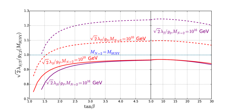
Figure 1: Variation of the ratios 2λS/gY2subscript𝜆𝑆subscript𝑔𝑌\sqrt{2}\lambda_{S}/g_{Y} and 2λT/g22subscript𝜆𝑇subscript𝑔2\sqrt{2}\lambda_{T}/g_{2} at the scale MSUSYsubscript𝑀SUSYM_{\rm SUSY} with tanβ𝛽\tan\beta, for MN=2=MSUSY,1010GeVsubscript𝑀𝑁2subscript𝑀SUSYsuperscript1010GeVM_{N=2}=M_{\rm SUSY},10^{10}\ \mathrm{GeV} and 1016superscript101610^{16} GeV.

At the scale Q=400𝑄400Q=400 GeV, we find gY=0.37,g2=0.64±0.01formulae-sequencesubscript𝑔𝑌0.37subscript𝑔2plus-or-minus0.640.01g_{Y}=0.37,g_{2}=0.64\pm 0.01. These are barely different at the SUSY scale and vary little with MN=2subscript𝑀𝑁2M_{N=2}, but we do find some dependence of the ratios 2λS/gY,2λT/g22subscript𝜆𝑆subscript𝑔𝑌2subscript𝜆𝑇subscript𝑔2\sqrt{2}\lambda_{S}/g_{Y},\sqrt{2}\lambda_{T}/g_{2} on this scale, which we give in figure 1. The values in the plot were taken with a common supersymmetric scale of MSUSY=3subscript𝑀SUSY3M_{\rm SUSY}=3 TeV and have essentially no dependence on mAsubscript𝑚𝐴m_{A}.

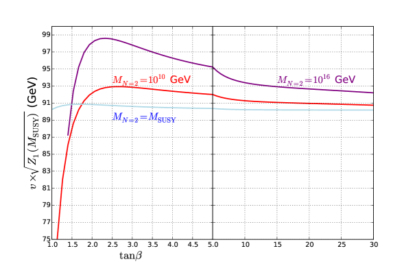
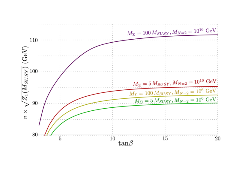
An alternative way of visualising this information is in the quantity Z1subscript𝑍1Z_{1} evaluated at the SUSY scale. Since our model is always very near alignment, this gives the “tree-level” Higgs mass and so in figure 2 we plot vZ1(MSUSY)𝑣subscript𝑍1subscript𝑀SUSYv\sqrt{Z_{1}(M_{\rm SUSY})}. We see that for MN=2=MSUSYsubscript𝑀𝑁2subscript𝑀SUSYM_{N=2}=M_{\rm SUSY} this is always essentially MZsubscript𝑀𝑍M_{Z}, while as we increase MN=2subscript𝑀𝑁2M_{N=2} we obtain a further enhancement to the Higgs mass at small tanβ1.5greater-than-or-equivalent-to𝛽1.5\tan\beta\gtrsim 1.5.

Refer to caption
Figure 2: v×Z1(MSUSY)𝑣subscript𝑍1subscript𝑀SUSYv\times\sqrt{Z_{1}(M_{\rm SUSY})} against tanβ𝛽\tan\beta for MN=2=MSUSY,1010subscript𝑀𝑁2subscript𝑀SUSYsuperscript1010M_{N=2}=M_{\rm SUSY},10^{10} GeV and 1016superscript101610^{16} GeV, which corresponds to the “tree-level” value of the Higgs mass before we take running from MSUSYsubscript𝑀SUSYM_{\rm SUSY} (or equivalently the SUSY corrections at MZsubscript𝑀𝑍M_{Z}) into account (we take v=246𝑣246v=246 GeV in the figure). We see that increasing MN=2subscript𝑀𝑁2M_{N=2} increases the Higgs mass, particularly for small tanβ>1.5𝛽1.5\tan\beta>1.5.

If we were to include no further corrections, then the value of Z6subscript𝑍6Z_{6} at MSUSYsubscript𝑀SUSYM_{\rm SUSY} would be given by

Z6(MSUSY)=subscript𝑍6subscript𝑀SUSYabsent\displaystyle Z_{6}(M_{\rm SUSY})= 14s2βc2β[gY2(2λS2/gY21)+g22(2λT2/g221)].14subscript𝑠2𝛽subscript𝑐2𝛽delimited-[]superscriptsubscript𝑔𝑌22superscriptsubscript𝜆𝑆2superscriptsubscript𝑔𝑌21superscriptsubscript𝑔222superscriptsubscript𝜆𝑇2superscriptsubscript𝑔221\displaystyle\frac{1}{4}s_{2\beta}c_{2\beta}\bigg{[}g_{Y}^{2}(2\lambda_{S}^{2}/g_{Y}^{2}-1)+g_{2}^{2}(2\lambda_{T}^{2}/g_{2}^{2}-1)\bigg{]}. (4.3)

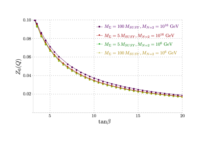
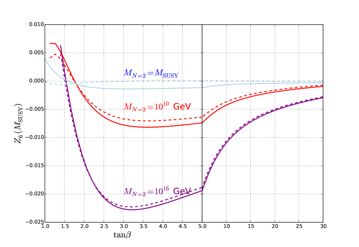
Crucially then we see that for MN=2>MSUSYsubscript𝑀𝑁2subscript𝑀SUSYM_{N=2}>M_{\rm SUSY} this is dominated by the relative positive shift in λTsubscript𝜆𝑇\lambda_{T}, which in turn yields a negative contribution to Z6subscript𝑍6Z_{6}. The results from our scans for the value of Z6subscript𝑍6Z_{6} at the SUSY scale almost exactly correspond to the above equation, which we plot in figure 3. The differences (particularly the tiny difference from zero for the N=2𝑁2N=2 scale equal to MSUSYsubscript𝑀SUSYM_{\rm SUSY}) come from the tree-level and loop-level shifts.
Refer to caption
Figure 3: Z6(MSUSY)subscript𝑍6subscript𝑀SUSYZ_{6}(M_{\rm SUSY}) against tanβ𝛽\tan\beta for MN=2=MSUSY,1010GeVsubscript𝑀𝑁2subscript𝑀SUSYsuperscript1010GeVM_{N=2}=M_{\rm SUSY},10^{10}\ \mathrm{GeV} and 1016superscript101610^{16} GeV, which corresponds to just the contributions to Z6subscript𝑍6Z_{6} from the running of λS,Tsubscript𝜆𝑆𝑇\lambda_{S,T} and the threshold corrections. The solid lines show the full value of Z6subscript𝑍6Z_{6}, while the dashed lines are just those given by equation (4.3), i.e. without threshold corrections.

4.2 Running below MSUSYsubscript𝑀SUSYM_{\rm SUSY}

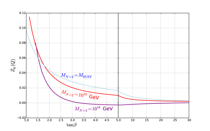
Once we include the two-loop running below MSUSYsubscript𝑀SUSYM_{\rm SUSY}, the picture changes substantially. This is dominated by the effects of the stops via their absence from the RGEs; we plot the results of Z6subscript𝑍6Z_{6} for the same scan as in figure 3 at the scale of our low-energy theory in figure 4.
Refer to caption
Figure 4: Z6(Q)subscript𝑍6𝑄Z_{6}(Q) against tanβ𝛽\tan\beta, where Q=400𝑄400Q=400 GeV is our low-energy matching scale. We find that the model shows good alignment for all values of tanβ>1.5𝛽1.5\tan\beta>1.5, with the surprising conclusion that raising the N=2𝑁2N=2 scale improves the alignment.

Interestingly, the results can be understood by following the reasoning of the hMSSM[74]/h2MSSM [73] treatment. In that framework, the quantum corrections to the Higgs mass are assumed to be dominated by the (2,2)22(2,2) component – and further that we can neglect the contributions to the other components compared to the tree-level ones. We shall first review what happens in the hMSSM and then apply the analysis to our case.

4.2.1 (Lack of) alignment in the hMSSM

In the hMSSM [74], we have λ2=MZ2+ϵv2subscript𝜆2superscriptsubscript𝑀𝑍2italic-ϵsuperscript𝑣2\lambda_{2}=\frac{M_{Z}^{2}+\epsilon}{v^{2}}, where ϵitalic-ϵ\epsilon encodes the loop corrections (dominated by stops), and all other terms are taken to have their tree-level values, giving the neutral Higgs mass matrix in the alignment basis of

mh,H2=(MZ2c2β2+ϵsβ4MZ2s2βc2β+sβ3cβϵMZ2s2βc2β+sβ3cβϵmA2+MZ2s2β2+sβ2cβ2ϵ).superscriptsubscript𝑚𝐻2superscriptsubscript𝑀𝑍2superscriptsubscript𝑐2𝛽2italic-ϵsuperscriptsubscript𝑠𝛽4superscriptsubscript𝑀𝑍2subscript𝑠2𝛽subscript𝑐2𝛽superscriptsubscript𝑠𝛽3subscript𝑐𝛽italic-ϵsuperscriptsubscript𝑀𝑍2subscript𝑠2𝛽subscript𝑐2𝛽superscriptsubscript𝑠𝛽3subscript𝑐𝛽italic-ϵsuperscriptsubscript𝑚𝐴2superscriptsubscript𝑀𝑍2superscriptsubscript𝑠2𝛽2superscriptsubscript𝑠𝛽2superscriptsubscript𝑐𝛽2italic-ϵ\displaystyle m_{h,H}^{2}=\left(\begin{array}[]{cc}M_{Z}^{2}c_{2\beta}^{2}+\epsilon s_{\beta}^{4}&-M_{Z}^{2}s_{2\beta}c_{2\beta}+s_{\beta}^{3}c_{\beta}\epsilon\\ -M_{Z}^{2}s_{2\beta}c_{2\beta}+s_{\beta}^{3}c_{\beta}\epsilon&m_{A}^{2}+M_{Z}^{2}s_{2\beta}^{2}+s_{\beta}^{2}c_{\beta}^{2}\epsilon\end{array}\right). (4.6)

Now let us suppose that we tune the values to obtain alignment. We then have

MZ2s2βc2β+sβ3cβϵ=superscriptsubscript𝑀𝑍2subscript𝑠2𝛽subscript𝑐2𝛽superscriptsubscript𝑠𝛽3subscript𝑐𝛽italic-ϵabsent\displaystyle-M_{Z}^{2}s_{2\beta}c_{2\beta}+s_{\beta}^{3}c_{\beta}\epsilon= 00\displaystyle 0
MZ2c2β2+ϵsβ4=superscriptsubscript𝑀𝑍2superscriptsubscript𝑐2𝛽2italic-ϵsuperscriptsubscript𝑠𝛽4absent\displaystyle M_{Z}^{2}c_{2\beta}^{2}+\epsilon s_{\beta}^{4}= mh2superscriptsubscript𝑚2\displaystyle m_{h}^{2} (4.7)

which leads to

c2β=subscript𝑐2𝛽absent\displaystyle c_{2\beta}= mh2MZ2>1orcβ=0,formulae-sequencesuperscriptsubscript𝑚2superscriptsubscript𝑀𝑍21orsubscript𝑐𝛽0\displaystyle\frac{m_{h}^{2}}{M_{Z}^{2}}>1\qquad\mathrm{or}\qquad c_{\beta}=0, (4.8)

i.e. it is impossible to achieve alignment without decoupling or going to the large tanβ𝛽\tan\beta limit with these approximations. If we do not neglect the other contributions to Z6subscript𝑍6Z_{6}, in the case of exact alignment we then have

0=Z6=0subscript𝑍6absent\displaystyle 0=Z_{6}= 1v2tβ(mh2MZ2c2β)sβcβ(cβ2δλ1c2βδλ345)1superscript𝑣2subscript𝑡𝛽superscriptsubscript𝑚2superscriptsubscript𝑀𝑍2subscript𝑐2𝛽subscript𝑠𝛽subscript𝑐𝛽superscriptsubscript𝑐𝛽2𝛿subscript𝜆1subscript𝑐2𝛽𝛿subscript𝜆345\displaystyle\frac{1}{v^{2}t_{\beta}}(m_{h}^{2}-M_{Z}^{2}c_{2\beta})-s_{\beta}c_{\beta}(c_{\beta}^{2}\delta\lambda_{1}-c_{2\beta}\delta\lambda_{345})
0=0absent\displaystyle 0= (mh2MZ2c2β)v2sβ2(cβ2δλ1c2βδλ345)superscriptsubscript𝑚2superscriptsubscript𝑀𝑍2subscript𝑐2𝛽superscript𝑣2superscriptsubscript𝑠𝛽2superscriptsubscript𝑐𝛽2𝛿subscript𝜆1subscript𝑐2𝛽𝛿subscript𝜆345\displaystyle(m_{h}^{2}-M_{Z}^{2}c_{2\beta})-v^{2}s_{\beta}^{2}(c_{\beta}^{2}\delta\lambda_{1}-c_{2\beta}\delta\lambda_{345}) (4.9)

Since we expect λ1,λ345λ2much-less-thansubscript𝜆1subscript𝜆345subscript𝜆2\lambda_{1},\lambda_{345}\ll\lambda_{2}, and for tβ>1subscript𝑡𝛽1t_{\beta}>1 we have sβ2>cβ2,sβ2>|c2β|formulae-sequencesuperscriptsubscript𝑠𝛽2superscriptsubscript𝑐𝛽2superscriptsubscript𝑠𝛽2subscript𝑐2𝛽s_{\beta}^{2}>c_{\beta}^{2},s_{\beta}^{2}>|c_{2\beta}|, this is still impossible to satisfy. 444In the full MSSM the radiative corrections to λ345subscript𝜆345\lambda_{345} and λ7subscript𝜆7\lambda_{7} – which we are neglecting – can be large enough to allow alignment for tanβ10greater-than-or-equivalent-to𝛽10\tan\beta\gtrsim 10 [6, 86]. However, this also requires significant stop mixing, which we do not have in our model.. However, we will find that for our scenario things are somewhat better.

4.2.2 Alignment in the Dirac-gaugino model

Using the expressions (2.20) for the quartic couplings, we can rewrite

λ1subscript𝜆1absent\displaystyle\lambda_{1}\equiv MZ2v2+δλ1,λ2MZ2v2+ϵv2,superscriptsubscript𝑀𝑍2superscript𝑣2𝛿subscript𝜆1subscript𝜆2superscriptsubscript𝑀𝑍2superscript𝑣2italic-ϵsuperscript𝑣2\displaystyle\frac{M_{Z}^{2}}{v^{2}}+\delta\lambda_{1},\qquad\lambda_{2}\equiv\frac{M_{Z}^{2}}{v^{2}}+\frac{\epsilon}{v^{2}},
λ345subscript𝜆345absent\displaystyle\lambda_{345}\equiv MZ2v2+12(2λS2gY2)+12(2λT2g22)+δλ345.superscriptsubscript𝑀𝑍2superscript𝑣2122superscriptsubscript𝜆𝑆2superscriptsubscript𝑔𝑌2122superscriptsubscript𝜆𝑇2superscriptsubscript𝑔22𝛿subscript𝜆345\displaystyle\frac{M_{Z}^{2}}{v^{2}}+\frac{1}{2}(2\lambda_{S}^{2}-g_{Y}^{2})+\frac{1}{2}(2\lambda_{T}^{2}-g_{2}^{2})+\delta\lambda_{345}. (4.10)

This leads to

Z1v2=subscript𝑍1superscript𝑣2absent\displaystyle Z_{1}v^{2}= MZ2+ϵsβ4+δλ1cβ4+12δλ345s2β2+v2[(2λS2gY2)+(2λT2g22)]sβ2cβ2superscriptsubscript𝑀𝑍2italic-ϵsuperscriptsubscript𝑠𝛽4𝛿subscript𝜆1superscriptsubscript𝑐𝛽412𝛿subscript𝜆345superscriptsubscript𝑠2𝛽2superscript𝑣2delimited-[]2superscriptsubscript𝜆𝑆2superscriptsubscript𝑔𝑌22superscriptsubscript𝜆𝑇2superscriptsubscript𝑔22superscriptsubscript𝑠𝛽2superscriptsubscript𝑐𝛽2\displaystyle M_{Z}^{2}+\epsilon s_{\beta}^{4}+\delta\lambda_{1}c_{\beta}^{4}+\frac{1}{2}\delta\lambda_{345}s_{2\beta}^{2}+v^{2}\bigg{[}(2\lambda_{S}^{2}-g_{Y}^{2})+(2\lambda_{T}^{2}-g_{2}^{2})\bigg{]}s_{\beta}^{2}c_{\beta}^{2}
Z6v2=subscript𝑍6superscript𝑣2absent\displaystyle Z_{6}v^{2}= sβ3cβϵv2sβcβ(cβ2δλ1c2βδλ345)+12c2βsβcβv2[(2λS2gY2)+(2λT2g22)].superscriptsubscript𝑠𝛽3subscript𝑐𝛽italic-ϵsuperscript𝑣2subscript𝑠𝛽subscript𝑐𝛽superscriptsubscript𝑐𝛽2𝛿subscript𝜆1subscript𝑐2𝛽𝛿subscript𝜆34512subscript𝑐2𝛽subscript𝑠𝛽subscript𝑐𝛽superscript𝑣2delimited-[]2superscriptsubscript𝜆𝑆2superscriptsubscript𝑔𝑌22superscriptsubscript𝜆𝑇2superscriptsubscript𝑔22\displaystyle s_{\beta}^{3}c_{\beta}\epsilon-v^{2}s_{\beta}c_{\beta}(c_{\beta}^{2}\delta\lambda_{1}-c_{2\beta}\delta\lambda_{345})+\frac{1}{2}c_{2\beta}s_{\beta}c_{\beta}v^{2}\bigg{[}(2\lambda_{S}^{2}-g_{Y}^{2})+(2\lambda_{T}^{2}-g_{2}^{2})\bigg{]}. (4.11)

The corrections δλi𝛿subscript𝜆𝑖\delta\lambda_{i} can be interpreted as either coming from running the couplings between the scale MSUSYsubscript𝑀SUSYM_{\rm SUSY} and Q𝑄Q, or alternatively from integrating out the supersymmetric particles at the scale Q𝑄Q. In the latter case we can obtain an estimate of their values from the expressions (3.5) and see that they are typically suppressed relative to ϵ/v2italic-ϵsuperscript𝑣2\epsilon/v^{2} by a numerical factor and also the ratio of the electroweak gauge coupling to the strong gauge coupling or top Yukawa, and we find that we can therefore continue with the hMSSM approximation and neglect them. However, the effect from the running of λS,λTsubscript𝜆𝑆subscript𝜆𝑇\lambda_{S},\lambda_{T} is non-negligible: eliminating ϵitalic-ϵ\epsilon in exchange for the Higgs mass and defining

δ^λ34512(2λS2gY2)+12(2λT2g22)^𝛿subscript𝜆345122superscriptsubscript𝜆𝑆2superscriptsubscript𝑔𝑌2122superscriptsubscript𝜆𝑇2superscriptsubscript𝑔22\displaystyle\hat{\delta}\lambda_{345}\equiv\frac{1}{2}(2\lambda_{S}^{2}-g_{Y}^{2})+\frac{1}{2}(2\lambda_{T}^{2}-g_{2}^{2}) (4.12)

we have

Z6=subscript𝑍6absent\displaystyle Z_{6}= sβcβv2(mA2sβ2+MZ2cβ2mh2)[(mA2mh2)(mh2MZ2)v2δ^λ345(mA2sβ2MZ2cβ2+mh2c2β)+v4cβ2sβ2(δ^λ345)2]subscript𝑠𝛽subscript𝑐𝛽superscript𝑣2superscriptsubscript𝑚𝐴2superscriptsubscript𝑠𝛽2superscriptsubscript𝑀𝑍2superscriptsubscript𝑐𝛽2superscriptsubscript𝑚2delimited-[]superscriptsubscript𝑚𝐴2superscriptsubscript𝑚2superscriptsubscript𝑚2superscriptsubscript𝑀𝑍2superscript𝑣2^𝛿subscript𝜆345superscriptsubscript𝑚𝐴2superscriptsubscript𝑠𝛽2superscriptsubscript𝑀𝑍2superscriptsubscript𝑐𝛽2superscriptsubscript𝑚2subscript𝑐2𝛽superscript𝑣4superscriptsubscript𝑐𝛽2superscriptsubscript𝑠𝛽2superscript^𝛿subscript𝜆3452\displaystyle\frac{s_{\beta}c_{\beta}}{v^{2}(m_{A}^{2}s_{\beta}^{2}+M_{Z}^{2}c_{\beta}^{2}-m_{h}^{2})}\bigg{[}(m_{A}^{2}-m_{h}^{2})(m_{h}^{2}-M_{Z}^{2})-v^{2}\hat{\delta}\lambda_{345}\bigg{(}m_{A}^{2}s_{\beta}^{2}-M_{Z}^{2}c_{\beta}^{2}+m_{h}^{2}c_{2\beta}\bigg{)}+v^{4}c_{\beta}^{2}s_{\beta}^{2}(\hat{\delta}\lambda_{345})^{2}\bigg{]}
\displaystyle\approx 0.12tβ12tβ1+tβ2[(2λS2gY2)+(2λT2g22)].0.12subscript𝑡𝛽12subscript𝑡𝛽1superscriptsubscript𝑡𝛽2delimited-[]2superscriptsubscript𝜆𝑆2superscriptsubscript𝑔𝑌22superscriptsubscript𝜆𝑇2superscriptsubscript𝑔22\displaystyle\frac{0.12}{t_{\beta}}-\frac{1}{2}\frac{t_{\beta}}{1+t_{\beta}^{2}}\bigg{[}(2\lambda_{S}^{2}-g_{Y}^{2})+(2\lambda_{T}^{2}-g_{2}^{2})\bigg{]}. (4.13)

We shall later give the expressions for eliminating λ2subscript𝜆2\lambda_{2} and calculating Z6subscript𝑍6Z_{6} in any THDM with general λi,i=14subscript𝜆𝑖𝑖14\lambda_{i},i=1...4 in equations (6.5) and (6.6).

A comparison of the above formula with the curves in figure 4 shows that this gives a reasonable fit. In the case of MN=2=MSUSYsubscript𝑀𝑁2subscript𝑀SUSYM_{N=2}=M_{\rm SUSY} the expression is particularly simple, but in the other cases we need to take account of the varation of 2λS(MSUSY),2λT(MSUSY)2subscript𝜆𝑆subscript𝑀SUSY2subscript𝜆𝑇subscript𝑀SUSY\sqrt{2}\lambda_{S}(M_{\rm SUSY}),\sqrt{2}\lambda_{T}(M_{\rm SUSY}) with tanβ𝛽\tan\beta that can be seen in figure 1.

The main conclusion that can be drawn from the above formula is that the misalignment coming from the squark corrections required to enhance the Higgs mass can be compensated by the effect of running λS,λTsubscript𝜆𝑆subscript𝜆𝑇\lambda_{S},\lambda_{T}. Indeed, we see from figure 4 that for MN=2=1016subscript𝑀𝑁2superscript1016M_{N=2}=10^{16} GeV, Z6subscript𝑍6Z_{6} is essentially vanishing for tanβ3greater-than-or-equivalent-to𝛽3\tan\beta\gtrsim 3. From the curves in the figure, we see that increasing the N=2𝑁2N=2 scale causes a partial or total cancellation of the misalignment contributions, meaning that the Higgs boson is accidentally very Standard-Model-like, independent of the mass of the heavy Higgs! This is the main result of the paper.

4.3 Higgs mass bounds on the SUSY scale

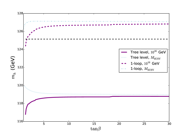
Finally we consider the effect of the loop corrections in the low-energy theory on the Higgs mass (i.e. those coming from the Higgs sector itself, the top and the electroweakinos). In figure 5 we show the tree-level and one-loop values for the Higgs mass as we vary tanβ𝛽\tan\beta (with MSUSYsubscript𝑀SUSYM_{\rm SUSY} fixed to ensure mh=125.15subscript𝑚125.15m_{h}=125.15 GeV at two loops). We find a significant upward shift of about 777 GeV at one-loop, and then a downward shift of about 111 or 222 GeV from one to two loops. Note that we can interpret the “tree-level” Higgs mass as the loop-level Higgs mass in the full Dirac gaugino model including the effects of the stops and gluinos (which in the EFT formalism appear via the RGEs, rather than fixed-order diagrams).

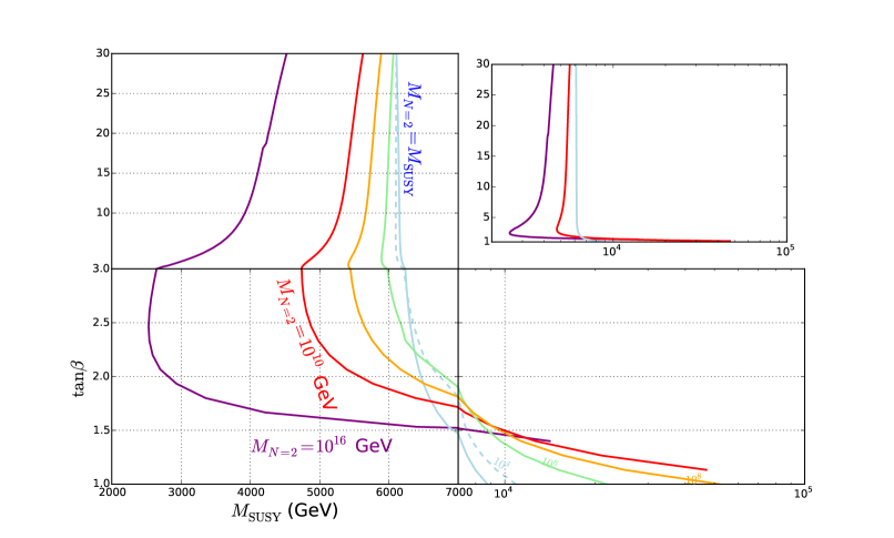
In figure 6 we show the final curve of tanβ𝛽\tan\beta against MSUSYsubscript𝑀SUSYM_{\rm SUSY}, for different values of the N=2𝑁2N=2 scale between MSUSYsubscript𝑀SUSYM_{\rm SUSY} and 1016superscript101610^{16} GeV.

The plot shows that there is a minimum for MSUSYsubscript𝑀SUSYM_{\rm SUSY} around tanβ2similar-to-or-equals𝛽2\tan\beta\simeq 2 or 333, particularly for larger values of MN=2subscript𝑀𝑁2M_{N=2}, which can be understood in terms of the splitting of λTsubscript𝜆𝑇\lambda_{T} from its N=2𝑁2N=2 value and the consequent boost to the Higgs mass, which can be clearly seen in figure 2.

The results in figure 6 contrast starkly with the MSSM case matched onto the 2HDM as shown in e.g. [87]: due to the enhancement to the Higgs mass from the new couplings already seen in figure 2 we have a much lower SUSY scale. On the other hand, there are significant differences from the values quoted in [73] which are most closely related to the case MN=2=MSUSYsubscript𝑀𝑁2subscript𝑀SUSYM_{N=2}=M_{\rm SUSY}; here of course we have light electroweakinos, although the largest difference is the significantly more accurate EFT calculation employed here.
Refer to caption
Figure 5: Effect of loop corrections in the low-energy theory on the Higgs mass. The tree-level and one-loop values for the Higgs mass are shown against tanβ𝛽\tan\beta for N=2𝑁2N=2 scales of the stop scale (MSUSYsubscript𝑀SUSYM_{\rm SUSY}) and 1016superscript101610^{16} GeV; the two-loop value of the Higgs mass is fixed to the black dotted line.
Refer to caption
Figure 6: SUSY scale that fits mh=125.2subscript𝑚125.2m_{h}=125.2 GeV against tanβ𝛽\tan\beta. The cases MN=2={MSUSY,1010GeV,1016GeV}subscript𝑀𝑁2subscript𝑀SUSYsuperscript1010GeVsuperscript1016GeVM_{N=2}=\{M_{\rm SUSY},10^{10}\ \mathrm{GeV},10^{16}\ \mathrm{GeV}\} are the solid lines in blue, red and purple respectively and are labelled in full; the cases MN=2={104,106,108}subscript𝑀𝑁2superscript104superscript106superscript108M_{N=2}=\{10^{4},10^{6},10^{8}\} GeV are respectively shown in blue dashed, solid green and solid orange curves and only labelled with {104,106,108}superscript104superscript106superscript108\{10^{4},10^{6},10^{8}\}. Due to the large range of scales MSUSYsubscript𝑀SUSYM_{\rm SUSY} values for small tanβ𝛽\tan\beta and the little change for large tanβ𝛽\tan\beta we have split the plot into three quadrants to show the values more clearly, but for comparison we give an inset graph showing the three curves MN=2={MSUSY,1010GeV,1016GeV}subscript𝑀𝑁2subscript𝑀SUSYsuperscript1010GeVsuperscript1016GeVM_{N=2}=\{M_{\rm SUSY},10^{10}\ \mathrm{GeV},10^{16}\ \mathrm{GeV}\} with MSUSYsubscript𝑀SUSYM_{\rm SUSY} (GeV) on a logarithmic scale on the abscissa and tanβ𝛽\tan\beta on a linear scale on the ordinate.

5 Experimental constraints

Since our model realises excellent alignment, the light Higgs couplings are very nearly Standard-Model-like across the whole parameter space, and so there is no significant constraint from those – this is in contrast to e.g. the hMSSM scenario, where for low tanβ𝛽\tan\beta the Higgs couplings provided until recently the most important lower bound on the Heavy Higgs mass. However, there are still significant constraints on the parameter space coming from electroweak precision tests, flavour and direct searches, as we detail below.

5.1 Electroweak precision corrections

There are two contributions to the electroweak precision parameters: those coming from the high-energy theory, and those coming from the low-energy theory. In the high-energy theory there will be contributions at tree-level from the triplet scalars: they should obtain a vacuum expectation value, and in our EFT this manifests itself as generating effective operators.

In the limit of zero CP violation, and neglecting the terms AS,ATsubscript𝐴𝑆subscript𝐴𝑇A_{S},A_{T} we can write the effective operator arising from integrating out the triplet as quite simply

absent\displaystyle\mathcal{L}\supset 14mTP4tr[Dμ(σa[(2λTμ+g2mD2)HdσaHd+(g2mD22λTμ)HuσaHu])]214superscriptsubscript𝑚𝑇𝑃4trsuperscriptdelimited-[]subscript𝐷𝜇superscript𝜎𝑎delimited-[]2subscript𝜆𝑇𝜇subscript𝑔2subscript𝑚𝐷2superscriptsubscript𝐻𝑑superscript𝜎𝑎subscript𝐻𝑑subscript𝑔2subscript𝑚𝐷22subscript𝜆𝑇𝜇superscriptsubscript𝐻𝑢superscript𝜎𝑎subscript𝐻𝑢2\displaystyle\frac{1}{4m_{TP}^{4}}\mathrm{tr}\bigg{[}D_{\mu}\bigg{(}\sigma^{a}\big{[}(\sqrt{2}\lambda_{T}\mu+g_{2}m_{D2})H_{d}^{\dagger}\sigma^{a}H_{d}+(g_{2}m_{D2}-\sqrt{2}\lambda_{T}\mu)H_{u}^{\dagger}\sigma^{a}H_{u}\big{]}\bigg{)}\bigg{]}^{2} (5.1)

where we understand summation on the index a𝑎a and

Dμσa=σaμig2[Wμ,σa].subscript𝐷𝜇superscript𝜎𝑎superscript𝜎𝑎subscript𝜇𝑖subscript𝑔2subscript𝑊𝜇superscript𝜎𝑎\displaystyle D_{\mu}\sigma^{a}=\sigma^{a}\partial_{\mu}-ig_{2}[W_{\mu},\sigma^{a}]. (5.2)

When we give a vacuum expectation value to the Higgs, this translates into the constraint from the expectation value of the triplet:

Δρ=Δ𝜌absent\displaystyle\Delta\rho= ΔmW2mW2=v2mTP4(2λTμ+g2mD2c2β)2,Δsuperscriptsubscript𝑚𝑊2superscriptsubscript𝑚𝑊2superscript𝑣2superscriptsubscript𝑚𝑇𝑃4superscript2subscript𝜆𝑇𝜇subscript𝑔2subscript𝑚𝐷2subscript𝑐2𝛽2\displaystyle\frac{\Delta m_{W}^{2}}{m_{W}^{2}}=\frac{v^{2}}{m_{TP}^{4}}\bigg{(}\sqrt{2}\lambda_{T}\mu+g_{2}m_{D2}c_{2\beta}\bigg{)}^{2}, (5.3)

while the experimental best-fit value is [88]

Δρ=(3.7±2.3)×104.Δ𝜌plus-or-minus3.72.3superscript104\displaystyle\Delta\rho=(3.7\pm 2.3)\times 10^{-4}. (5.4)

For μ=500𝜇500\mu=500 GeV and an approximately N=2𝑁2N=2 value for λTsubscript𝜆𝑇\lambda_{T}, with small tanβ𝛽\tan\beta insisting that this contribution does not exceed the experimental bound by 3σ3𝜎3\sigma gives

mTP>1500GeVsubscript𝑚𝑇𝑃1500GeV\displaystyle m_{TP}>1500\ \mathrm{GeV} (5.5)

while simply saturating without exceeding the central best-fit value would limit instead mTP>2TeVsubscript𝑚𝑇𝑃2TeVm_{TP}>2\ \mathrm{TeV}.

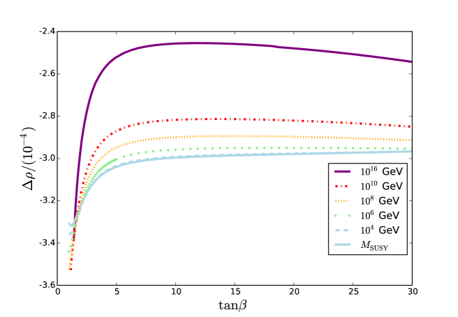
On the other hand, we also have a contribution from the electroweakinos at loop level, which increases as the Dirac mass/μ𝜇\mu-term become smaller. Hence they cannot be arbitrarily light. In figure 7 we plot the value of ΔρΔ𝜌\Delta\rho calculated in the low-energy theory for the scan values (4.1) and find that they are below the experimental limit across the whole parameter space.
Refer to caption
Figure 7: ΔρΔ𝜌\Delta\rho calculated at one-loop in the low-energy theory, for different values of MN=2subscript𝑀𝑁2M_{N=2} given in the legend. We see that the magnitude is roughly equal to the experimental error, and we are always well within 3σ3𝜎3\sigma of the experimental central value (which is anyway above the Standard Model value by 1.6σ1.6𝜎1.6\sigma).

5.2 Bounds on tanβ𝛽\tan\beta and mAsubscript𝑚𝐴m_{A}

The most stringent constraints on the parameter space of our model come from the searches for ppH/Aττ𝑝𝑝𝐻𝐴𝜏𝜏pp\rightarrow H/A\rightarrow\tau\tau at the LHC; and the decay Bsγ𝐵𝑠𝛾B\rightarrow s\gamma determined in [89], which bounds the charged Higgs mass to be heavier than 580580580 GeV independent of the value of tanβ𝛽\tan\beta (which in turn bounds the mass of the pseudoscalar Higgs to be above around 568568568 GeV).

Refer to caption
Figure 8: Bounds from ppH/Aτ+τ𝑝𝑝𝐻𝐴superscript𝜏superscript𝜏pp\rightarrow H/A\rightarrow\tau^{+}\tau^{-} (blue region) and Bsγ𝐵𝑠𝛾B\rightarrow s\gamma (red region, mA568less-than-or-similar-tosubscript𝑚𝐴568m_{A}\lesssim 568 GeV) interpreted in the mA/tanβsubscript𝑚𝐴𝛽m_{A}/\tan\beta plane for the hMSSM (taken from [90]) and our model.

The bounds from run 1 of the LHC were rather mild on the hMSSM: they restricted tanβ<8𝛽8\tan\beta<8 for low mAsubscript𝑚𝐴m_{A} (see e.g. [86, 91]). In [73] it was claimed that in the h2MSSM these bounds would apply unaltered; while it is true that the couplings to the pseudoscalar are the same in the h2MSSM and hMSSM, the “heavy” Higgs does have altered couplings at small mAsubscript𝑚𝐴m_{A} and tanβ𝛽\tan\beta – since it is more aligned. Since the production of the Heavy Higgs is dominated at small tanβ𝛽\tan\beta by gluon fusion, and at large tanβ𝛽\tan\beta by the bbH process, then we would expect some differences at small tanβ𝛽\tan\beta. However, recently, ATLAS produced a much enhanced bound [90] on gluon fusion and bbH production and then decay to τ𝜏\tau pairs; they also interpreted this in terms of the hMSSM. To compare to our model we computed Higgs production using SusHi [92, 93, 94, 95, 96, 97, 98] and rescaled the production cross-sections according to b-quark and gluon couplings computed in our SARAH/SPheno code, then multiplied by the tau decay branching fraction, and combined the bound assuming that the signals from H/A𝐻𝐴H/A production overlap for small mass differences. We show the result in figure 8, where we also show the bound from [90] on the hMSSM. We find almost no difference, except that the bound on our model is very slightly weaker once decays to the electroweakinos are permitted. However, the branching ratio to electroweakinos in that region is never significant enough to reduce the τ𝜏\tau decay fraction.

6 Alignment in the MRSSM

For completeness we now discuss the case of the MRSSM in the same limit as for the DG-MSSM. Since the tree-level THDM parameters are the same as those of the MSSM in the limit of large adjoint scalar and R-Higgs masses,555So therefore Z1,Z5,Z6subscript𝑍1subscript𝑍5subscript𝑍6Z_{1},Z_{5},Z_{6} are the same as in the MSSM case, i.e. equations (2.34) - (2.36) with λS=λT=0subscript𝜆𝑆subscript𝜆𝑇0\lambda_{S}=\lambda_{T}=0. there is no contribution to Z6subscript𝑍6Z_{6} from the running of the parameters λSu,d,λTu,dsubscript𝜆subscript𝑆𝑢𝑑subscript𝜆subscript𝑇𝑢𝑑\lambda_{S_{u,d}},\lambda_{T_{u,d}}. We can first write the neutral Higgs mass matrix as

mh,H2=(MZ2c2β2+v2ΔZ1MZ2s2βc2β+v2ΔZ6MZ2s2βc2β+v2ΔZ6mA2+MZ2s2β2+v2ΔZ5).superscriptsubscript𝑚𝐻2superscriptsubscript𝑀𝑍2superscriptsubscript𝑐2𝛽2superscript𝑣2Δsubscript𝑍1superscriptsubscript𝑀𝑍2subscript𝑠2𝛽subscript𝑐2𝛽superscript𝑣2Δsubscript𝑍6superscriptsubscript𝑀𝑍2subscript𝑠2𝛽subscript𝑐2𝛽superscript𝑣2Δsubscript𝑍6superscriptsubscript𝑚𝐴2superscriptsubscript𝑀𝑍2superscriptsubscript𝑠2𝛽2superscript𝑣2Δsubscript𝑍5\displaystyle m_{h,H}^{2}=\left(\begin{array}[]{cc}M_{Z}^{2}c_{2\beta}^{2}+v^{2}\Delta Z_{1}&-M_{Z}^{2}s_{2\beta}c_{2\beta}+v^{2}\Delta Z_{6}\\ -M_{Z}^{2}s_{2\beta}c_{2\beta}+v^{2}\Delta Z_{6}&m_{A}^{2}+M_{Z}^{2}s_{2\beta}^{2}+v^{2}\Delta Z_{5}\end{array}\right). (6.3)

If we consider the loop corrections due to λSu,d,λTu,dsubscript𝜆subscript𝑆𝑢𝑑subscript𝜆subscript𝑇𝑢𝑑\lambda_{S_{u,d}},\lambda_{T_{u,d}} to be small, then the analysis of alignment is identical to the MSSM case, and we can apply the hMSSM logic. However, if we instead take them to be non-negligible – such as in [54, 53, 65, 66] – then the contributions to λ2subscript𝜆2\lambda_{2} no longer dominate, and the hMSSM reasoning may no longer apply. On the other hand, the largest contribution from the other particles will still be to λ2subscript𝜆2\lambda_{2}, and so we can assume that

λ2=subscript𝜆2absent\displaystyle\lambda_{2}= MZ2+ϵv2,λ1=MZ2v2+δλ1superscriptsubscript𝑀𝑍2italic-ϵsuperscript𝑣2subscript𝜆1superscriptsubscript𝑀𝑍2superscript𝑣2𝛿subscript𝜆1\displaystyle\frac{M_{Z}^{2}+\epsilon}{v^{2}},\qquad\lambda_{1}=\frac{M_{Z}^{2}}{v^{2}}+\delta\lambda_{1}
λ5=subscript𝜆5absent\displaystyle\lambda_{5}= 0,λ345=λ34=MZ2v2+δλ34.0subscript𝜆345subscript𝜆34superscriptsubscript𝑀𝑍2superscript𝑣2𝛿subscript𝜆34\displaystyle 0,\qquad\lambda_{345}=\lambda_{34}=-\frac{M_{Z}^{2}}{v^{2}}+\delta\lambda_{34}. (6.4)

To eliminate ϵitalic-ϵ\epsilon, we eliminate λ2subscript𝜆2\lambda_{2} in terms of the Higgs mass, which for general λi,i=14subscript𝜆𝑖𝑖14\lambda_{i},i=1...4 (and λ5=λ6=λ7=0subscript𝜆5subscript𝜆6subscript𝜆70\lambda_{5}=\lambda_{6}=\lambda_{7}=0):

λ2v2sβ2+mA2cβ2=subscript𝜆2superscript𝑣2superscriptsubscript𝑠𝛽2superscriptsubscript𝑚𝐴2superscriptsubscript𝑐𝛽2absent\displaystyle\lambda_{2}v^{2}s_{\beta}^{2}+m_{A}^{2}c_{\beta}^{2}= mh2+sβ2cβ2(mA2λ34v2)2λ1v2cβ2+mA2sβ2mh2;superscriptsubscript𝑚2superscriptsubscript𝑠𝛽2superscriptsubscript𝑐𝛽2superscriptsuperscriptsubscript𝑚𝐴2subscript𝜆34superscript𝑣22subscript𝜆1superscript𝑣2superscriptsubscript𝑐𝛽2superscriptsubscript𝑚𝐴2superscriptsubscript𝑠𝛽2superscriptsubscript𝑚2\displaystyle m_{h}^{2}+\frac{s_{\beta}^{2}c_{\beta}^{2}(m_{A}^{2}-\lambda_{34}v^{2})^{2}}{\lambda_{1}v^{2}c_{\beta}^{2}+m_{A}^{2}s_{\beta}^{2}-m_{h}^{2}}; (6.5)

this can then be substituted into the expression for Z6subscript𝑍6Z_{6}:

Z6=subscript𝑍6absent\displaystyle Z_{6}= sβcβλ1v4cβ2+mA2v2sβ2mh2v2×\displaystyle-\frac{s_{\beta}c_{\beta}}{\lambda_{1}v^{4}c_{\beta}^{2}+m_{A}^{2}v^{2}s_{\beta}^{2}-m_{h}^{2}v^{2}}\times
[(λ1v2cβ2mh2)(λ1v2cβ2mh2+mA2λ34v2c2β)+λ34sβ2v2(mA2λ34cβ2v2)].delimited-[]subscript𝜆1superscript𝑣2superscriptsubscript𝑐𝛽2superscriptsubscript𝑚2subscript𝜆1superscript𝑣2superscriptsubscript𝑐𝛽2superscriptsubscript𝑚2superscriptsubscript𝑚𝐴2subscript𝜆34superscript𝑣2subscript𝑐2𝛽subscript𝜆34superscriptsubscript𝑠𝛽2superscript𝑣2superscriptsubscript𝑚𝐴2subscript𝜆34superscriptsubscript𝑐𝛽2superscript𝑣2\displaystyle\bigg{[}(\lambda_{1}v^{2}c_{\beta}^{2}-m_{h}^{2})(\lambda_{1}v^{2}c_{\beta}^{2}-m_{h}^{2}+m_{A}^{2}-\lambda_{34}v^{2}c_{2\beta})+\lambda_{34}s_{\beta}^{2}v^{2}(m_{A}^{2}-\lambda_{34}c_{\beta}^{2}v^{2})\bigg{]}. (6.6)

We give the loop corrections to the λisubscript𝜆𝑖\lambda_{i} from the adjoint scalars in appendix D, but in the simplified case of mT+=mT=mSR=mSI=MΣsubscript𝑚superscript𝑇subscript𝑚superscript𝑇subscript𝑚𝑆𝑅subscript𝑚𝑆𝐼subscript𝑀Σm_{T^{+}}=m_{T^{-}}=m_{SR}=m_{SI}=M_{\Sigma} and gY=g2=0subscript𝑔𝑌subscript𝑔20g_{Y}=g_{2}=0 we have, for matching at a scale μ𝜇\mu:

δλ1=𝛿subscript𝜆1absent\displaystyle\delta\lambda_{1}= 116π2logMΣ2μ2(5λTd4+2λSd2λTd2+λSd4)116superscript𝜋2superscriptsubscript𝑀Σ2superscript𝜇25superscriptsubscript𝜆subscript𝑇𝑑42superscriptsubscript𝜆subscript𝑆𝑑2superscriptsubscript𝜆subscript𝑇𝑑2superscriptsubscript𝜆subscript𝑆𝑑4\displaystyle\frac{1}{16\pi^{2}}\log\frac{M_{\Sigma}^{2}}{\mu^{2}}\bigg{(}5\lambda_{T_{d}}^{4}+2\lambda_{S_{d}}^{2}\lambda_{T_{d}}^{2}+\lambda_{S_{d}}^{4}\bigg{)}
δλ2=𝛿subscript𝜆2absent\displaystyle\delta\lambda_{2}= 116π2logMΣ2μ2(5λTu4+2λSu2λTu2+λSu4)116superscript𝜋2superscriptsubscript𝑀Σ2superscript𝜇25superscriptsubscript𝜆subscript𝑇𝑢42superscriptsubscript𝜆subscript𝑆𝑢2superscriptsubscript𝜆subscript𝑇𝑢2superscriptsubscript𝜆subscript𝑆𝑢4\displaystyle\frac{1}{16\pi^{2}}\log\frac{M_{\Sigma}^{2}}{\mu^{2}}\bigg{(}5\lambda_{T_{u}}^{4}+2\lambda_{S_{u}}^{2}\lambda_{T_{u}}^{2}+\lambda_{S_{u}}^{4}\bigg{)}
δλ3=𝛿subscript𝜆3absent\displaystyle\delta\lambda_{3}= 116π2logMΣ2μ2(5λTd2λTu2+λSdλSuλTdλTu+λSd2λSu2)116superscript𝜋2superscriptsubscript𝑀Σ2superscript𝜇25superscriptsubscript𝜆subscript𝑇𝑑2superscriptsubscript𝜆subscript𝑇𝑢2subscript𝜆subscript𝑆𝑑subscript𝜆subscript𝑆𝑢subscript𝜆subscript𝑇𝑑subscript𝜆subscript𝑇𝑢superscriptsubscript𝜆subscript𝑆𝑑2superscriptsubscript𝜆subscript𝑆𝑢2\displaystyle\frac{1}{16\pi^{2}}\log\frac{M_{\Sigma}^{2}}{\mu^{2}}\bigg{(}5\lambda_{T_{d}}^{2}\lambda_{T_{u}}^{2}+\lambda_{S_{d}}\lambda_{S_{u}}\lambda_{T_{d}}\lambda_{T_{u}}+\lambda_{S_{d}}^{2}\lambda_{S_{u}}^{2}\bigg{)}
δλ4=𝛿subscript𝜆4absent\displaystyle\delta\lambda_{4}= 116π2logMΣ2μ2(4λTd2λTu24λTdλTuλSdλSu).116superscript𝜋2superscriptsubscript𝑀Σ2superscript𝜇24superscriptsubscript𝜆subscript𝑇𝑑2superscriptsubscript𝜆subscript𝑇𝑢24subscript𝜆subscript𝑇𝑑subscript𝜆subscript𝑇𝑢subscript𝜆subscript𝑆𝑑subscript𝜆subscript𝑆𝑢\displaystyle\frac{1}{16\pi^{2}}\log\frac{M_{\Sigma}^{2}}{\mu^{2}}\bigg{(}-4\lambda_{T_{d}}^{2}\lambda_{T_{u}}^{2}-4\lambda_{T_{d}}\lambda_{T_{u}}\lambda_{S_{d}}\lambda_{S_{u}}\bigg{)}. (6.7)

If we then take (as in [54, 65, 66]) λSu=λSdλ,λTu=λTdΛformulae-sequencesubscript𝜆subscript𝑆𝑢subscript𝜆subscript𝑆𝑑𝜆subscript𝜆subscript𝑇𝑢subscript𝜆subscript𝑇𝑑Λ\lambda_{S_{u}}=-\lambda_{S_{d}}\equiv\lambda,\lambda_{T_{u}}=\lambda_{T_{d}}\equiv\Lambda, and allow an additional contribution ϵ/v2italic-ϵsuperscript𝑣2\epsilon/v^{2} to λ2subscript𝜆2\lambda_{2} from the stops, then we have

Z6=subscript𝑍6absent\displaystyle Z_{6}= 12s2βc2β(2MZ2v2+2Λ416π2logMΣ2μ2)+ϵv2sβ3cβ12subscript𝑠2𝛽subscript𝑐2𝛽2superscriptsubscript𝑀𝑍2superscript𝑣22superscriptΛ416superscript𝜋2superscriptsubscript𝑀Σ2superscript𝜇2italic-ϵsuperscript𝑣2superscriptsubscript𝑠𝛽3subscript𝑐𝛽\displaystyle-\frac{1}{2}s_{2\beta}c_{2\beta}\bigg{(}\frac{2M_{Z}^{2}}{v^{2}}+\frac{2\Lambda^{4}}{16\pi^{2}}\log\frac{M_{\Sigma}^{2}}{\mu^{2}}\bigg{)}+\frac{\epsilon}{v^{2}}s_{\beta}^{3}c_{\beta}
ΔZ1=Δsubscript𝑍1absent\displaystyle\Delta Z_{1}= 116π2logMΣ2μ2[λ4+2λ2Λ2+3Λ4+2Λ4c2β2]+ϵv2sβ4.116superscript𝜋2superscriptsubscript𝑀Σ2superscript𝜇2delimited-[]superscript𝜆42superscript𝜆2superscriptΛ23superscriptΛ42superscriptΛ4superscriptsubscript𝑐2𝛽2italic-ϵsuperscript𝑣2superscriptsubscript𝑠𝛽4\displaystyle\frac{1}{16\pi^{2}}\log\frac{M_{\Sigma}^{2}}{\mu^{2}}\bigg{[}\lambda^{4}+2\lambda^{2}\Lambda^{2}+3\Lambda^{4}+2\Lambda^{4}c_{2\beta}^{2}\bigg{]}+\frac{\epsilon}{v^{2}}s_{\beta}^{4}. (6.8)

We see that when the couplings λ,Λ𝜆Λ\lambda,\Lambda are large enough, the alignment will always be improved compared to the MSSM, because the enhancement to Z1subscript𝑍1Z_{1} is always greater than that to Z6subscript𝑍6Z_{6}. We note three cases of particular interest:

  1. 1.

    If we increase the contributions from the adjoint scalars to the point that we can neglect those from the stops, then we see that for small tanβ𝛽\tan\beta we will easily have alignment (in contrast to the MSSM case).

  2. 2.

    Alternatively, we could enhance the contributions from λ𝜆\lambda rather than ΛΛ\Lambda, since the former coupling does not contribute to Z6subscript𝑍6Z_{6}.

  3. 3.

    On the other hand, if we take the N=2𝑁2N=2 supersymmetric limit

    λTu=subscript𝜆subscript𝑇𝑢absent\displaystyle\lambda_{T_{u}}= λTd=g22,λSu=gY2,λSd=gY2,formulae-sequencesubscript𝜆subscript𝑇𝑑subscript𝑔22formulae-sequencesubscript𝜆subscript𝑆𝑢subscript𝑔𝑌2subscript𝜆subscript𝑆𝑑subscript𝑔𝑌2\displaystyle\lambda_{T_{d}}=\frac{g_{2}}{\sqrt{2}},\quad\lambda_{S_{u}}=\frac{g_{Y}}{\sqrt{2}},\quad\lambda_{S_{d}}=-\frac{g_{Y}}{\sqrt{2}}, (6.9)

    we find, using the expressions in appendix D (and no longer neglecting the gauge couplings):

    δλ1=𝛿subscript𝜆1absent\displaystyle\delta\lambda_{1}= 116π2logMΣ2μ214(3g24+2g22gY2+gY4)116superscript𝜋2superscriptsubscript𝑀Σ2superscript𝜇2143superscriptsubscript𝑔242superscriptsubscript𝑔22superscriptsubscript𝑔𝑌2superscriptsubscript𝑔𝑌4\displaystyle\frac{1}{16\pi^{2}}\log\frac{M_{\Sigma}^{2}}{\mu^{2}}\frac{1}{4}\bigg{(}3g_{2}^{4}+2g_{2}^{2}g_{Y}^{2}+g_{Y}^{4}\bigg{)}
    δλ2=𝛿subscript𝜆2absent\displaystyle\delta\lambda_{2}= δλ1𝛿subscript𝜆1\displaystyle\delta\lambda_{1}
    δλ3=𝛿subscript𝜆3absent\displaystyle\delta\lambda_{3}= 116π2logMΣ2μ214(3g242g22gY2+gY4)116superscript𝜋2superscriptsubscript𝑀Σ2superscript𝜇2143superscriptsubscript𝑔242superscriptsubscript𝑔22superscriptsubscript𝑔𝑌2superscriptsubscript𝑔𝑌4\displaystyle\frac{1}{16\pi^{2}}\log\frac{M_{\Sigma}^{2}}{\mu^{2}}\frac{1}{4}\bigg{(}3g_{2}^{4}-2g_{2}^{2}g_{Y}^{2}+g_{Y}^{4}\bigg{)}
    δλ4=𝛿subscript𝜆4absent\displaystyle\delta\lambda_{4}= 116π2logMΣ2μ2(g22gY2)116superscript𝜋2superscriptsubscript𝑀Σ2superscript𝜇2superscriptsubscript𝑔22superscriptsubscript𝑔𝑌2\displaystyle\frac{1}{16\pi^{2}}\log\frac{M_{\Sigma}^{2}}{\mu^{2}}\bigg{(}g_{2}^{2}g_{Y}^{2}\bigg{)} (6.10)

    giving

    δλ345=𝛿subscript𝜆345absent\displaystyle\delta\lambda_{345}= δλ1δλ,𝛿subscript𝜆1𝛿𝜆\displaystyle\delta\lambda_{1}\equiv\delta\lambda, (6.11)

    so there is no shift to Z6subscript𝑍6Z_{6} from the adjoint scalars, but we do have a shift to Z1subscript𝑍1Z_{1}, i.e

    ΔZ1=Δsubscript𝑍1absent\displaystyle\Delta Z_{1}= δλ,ΔZ6=0.𝛿𝜆Δsubscript𝑍60\displaystyle\delta\lambda,\qquad\Delta Z_{6}=0. (6.12)

    If the mass of the adjoint scalars is comparable to the mass of the stops, then this will however never be significant. On the other hand, if we take the adjoint scalars to be very heavy, then this indicates that we can have improved alignment relative to the MSSM. To quantify this, we can use our above expression for Z6subscript𝑍6Z_{6} (6.6):

    Z6=subscript𝑍6absent\displaystyle Z_{6}= sβcβ(MZ2v2+δλv4)cβ2+mA2v2sβ2mh2v2[Δ0+δλv2(mA2mh2+2cβ2MZ2)]subscript𝑠𝛽subscript𝑐𝛽superscriptsubscript𝑀𝑍2superscript𝑣2𝛿𝜆superscript𝑣4superscriptsubscript𝑐𝛽2superscriptsubscript𝑚𝐴2superscript𝑣2superscriptsubscript𝑠𝛽2superscriptsubscript𝑚2superscript𝑣2delimited-[]subscriptΔ0𝛿𝜆superscript𝑣2superscriptsubscript𝑚𝐴2superscriptsubscript𝑚22superscriptsubscript𝑐𝛽2superscriptsubscript𝑀𝑍2\displaystyle-\frac{s_{\beta}c_{\beta}}{(M_{Z}^{2}v^{2}+\delta\lambda v^{4})c_{\beta}^{2}+m_{A}^{2}v^{2}s_{\beta}^{2}-m_{h}^{2}v^{2}}\bigg{[}\Delta_{0}+\delta\lambda v^{2}(m_{A}^{2}-m_{h}^{2}+2c_{\beta}^{2}M_{Z}^{2})\bigg{]} (6.13)

    where

    Δ0=subscriptΔ0absent\displaystyle\Delta_{0}= mh2(mh2mA2MZ2(4cβ21))+MZ2c2β(mA2+2MZ2cβ2)superscriptsubscript𝑚2superscriptsubscript𝑚2superscriptsubscript𝑚𝐴2superscriptsubscript𝑀𝑍24superscriptsubscript𝑐𝛽21superscriptsubscript𝑀𝑍2subscript𝑐2𝛽superscriptsubscript𝑚𝐴22superscriptsubscript𝑀𝑍2superscriptsubscript𝑐𝛽2\displaystyle m_{h}^{2}(m_{h}^{2}-m_{A}^{2}-M_{Z}^{2}(4c_{\beta}^{2}-1))+M_{Z}^{2}c_{2\beta}(m_{A}^{2}+2M_{Z}^{2}c_{\beta}^{2}) (6.14)

    which is the numerator for the MSSM case. In the case that mA2mh2much-greater-thansuperscriptsubscript𝑚𝐴2superscriptsubscript𝑚2m_{A}^{2}\gg m_{h}^{2} (which corresponds to our case of interest – even though we would like mAsubscript𝑚𝐴m_{A} small enough to not entirely be in the decoupling limit), we therefore find

    Z6similar-to-or-equalssubscript𝑍6absent\displaystyle Z_{6}\simeq 1tβ[mh2MZ2c2βv2δλ].1subscript𝑡𝛽delimited-[]superscriptsubscript𝑚2superscriptsubscript𝑀𝑍2subscript𝑐2𝛽superscript𝑣2𝛿𝜆\displaystyle\frac{1}{t_{\beta}}\bigg{[}\frac{m_{h}^{2}-M_{Z}^{2}c_{2\beta}}{v^{2}}-\delta\lambda\bigg{]}. (6.15)

    For MΣ=100MSUSYsubscript𝑀Σ100subscript𝑀𝑆𝑈𝑆𝑌M_{\Sigma}=100M_{SUSY} (a rather extreme value) and matching at MSUSYsubscript𝑀𝑆𝑈𝑆𝑌M_{SUSY} we therefore find

    δλsimilar-to-or-equals𝛿𝜆absent\displaystyle\delta\lambda\simeq 0.04mh2v2,0.04superscriptsubscript𝑚2superscript𝑣2\displaystyle 0.04\,\frac{m_{h}^{2}}{v^{2}}, (6.16)

    and so the deviation of Z6subscript𝑍6Z_{6} from the MSSM value due to the adjoint scalars should be less than 4%percent44\%. On the other hand, as we shall see below, they can still have a significant effect on the SUSY scale.

Therefore, from the analysis above, in all three cases of interest, the alignment will never be as good as for our minimal Dirac gaugino model, because of the tree-level contribution to misalignment: we shall illustrate this for the N=2𝑁2N=2 case in the next subsection.

6.1 Numerical analysis of an N=2𝑁2N=2 MRSSM

To compare with our previous analysis of the DG-MSSM, here we present a simplified numerical analysis for an N=2𝑁2N=2 MRSSM, as defined in point 3 above and equation (6.9). From our estimations above, the alignment should only differ from the MSSM when relatively extreme values are taken for the adjoint scalar masses, and so to perform a precise analysis we would need to have a tower of effective field theories and the appropriate threshold corrections. Instead we decided to neglect all loop-level threshold corrections other than those from the adjoint scalars (although we use 2-loop RGEs throughout) and performed a simple analysis where the low energy model was approximated by the Standard Model and type-II two-Higgs doublet model. In this way we should obtain an idea of how the adjoint scalar masses cause the SUSY scale and alignment to vary from the predictions of the MSSM.

6.1.1 Procedure

Two-loop Standard Model matching values were implemented at mtsubscript𝑚𝑡m_{t} for the standard model gauge, Yukawa, and Higgs quartic couplings from [99] and a two-loop Standard Model running was performed up to an intermediate scale Q=600𝑄600Q=600 GeV, where the λi(Q)subscript𝜆𝑖𝑄\lambda_{i}(Q) couplings were given approximate values to be determined through future iterations between the scales Q𝑄Q and MN=2subscript𝑀𝑁2M_{N=2}. The two-Higgs doublet model 2-loop running was implemented up to the supersymmetry breaking scale defining the leading squark masses, MSUSYsubscript𝑀𝑆𝑈𝑆𝑌M_{SUSY}, where guesses were made for the inputs of the parameters λS,Tu,dsubscript𝜆𝑆subscript𝑇𝑢𝑑\lambda_{S,T_{u,d}}. The MRSSM was then run to 2-loops to some high scale MN=2subscript𝑀𝑁2M_{N=2} where the N=2𝑁2N=2 boundary conditions (6.9) were implemented. All two-loop beta functions were generated in 𝚂𝙰𝚁𝙰𝙷𝚂𝙰𝚁𝙰𝙷\tt{SARAH}, and the value of mAtree=600superscriptsubscript𝑚𝐴𝑡𝑟𝑒𝑒600m_{A}^{tree}=600 GeV was taken as in the minimal Dirac gaugino case. In this simplified model, as the electroweakinos are not taken to be light, the intermediate scale Q𝑄Q is taken to match the choice of heavy Higgs mass. Indeed, with these choices we should understand the Dirac gaugino masses mDY,mD2,mD3subscript𝑚𝐷𝑌subscript𝑚𝐷2subscript𝑚𝐷3m_{DY},m_{D2},m_{D3} and the higgsino mass to be at MSUSYsubscript𝑀SUSYM_{\rm SUSY}, and also the masses of the R-Higgs fields Ru,dsubscript𝑅𝑢𝑑R_{u,d} should be at that scale, because we do not implement any threshold corrections from those fields (leaving these to future work).

On the run down, λi(MSUSY)subscript𝜆𝑖subscript𝑀𝑆𝑈𝑆𝑌\lambda_{i}(M_{SUSY}) were matched to the 1-loop threshold corrections coming from the heavy S,T𝑆𝑇S,T scalars as given in appendix D, taking the adjoint scalars to be degenerate with mass MΣsubscript𝑀ΣM_{\Sigma}. This process was iterated, re-matching the gauge and Yukawa couplings onto their 2-loop Standard Model running values at the scale Q𝑄Q, while the λisubscript𝜆𝑖\lambda_{i} and λS,Tu,dsubscript𝜆𝑆subscript𝑇𝑢𝑑\lambda_{S,T_{u,d}} couplings were matched to the outputs from the previous running until their values converged. Finally, the λisubscript𝜆𝑖\lambda_{i} parameters were mapped back onto the Higgs quartic coupling using λ(Q)=Z1(Q)𝜆𝑄subscript𝑍1𝑄\lambda(Q)=Z_{1}(Q) and the Standard Model couplings were run back down to mtsubscript𝑚𝑡m_{t}. The correct Higgs mass was selected from the criterion λ(mt)=0.252±0.002𝜆subscript𝑚𝑡plus-or-minus0.2520.002\lambda(m_{t})=0.252\pm 0.002, corresponding to a pole Higgs mass of mh=125±0.5subscript𝑚plus-or-minus1250.5m_{h}=125\pm 0.5 GeV.

This process was executed for scans over the values tanβ[2,20]𝛽220\tan\beta\in[2,20]; MSUSY[0.5,10]subscript𝑀𝑆𝑈𝑆𝑌0.510M_{SUSY}\in[0.5,10] TeV; MΣ={5,10,100}MSUSYsubscript𝑀Σ510100subscript𝑀𝑆𝑈𝑆𝑌M_{\Sigma}=\left\{5,10,100\right\}M_{SUSY} and MN=2={106,1010,1016}subscript𝑀𝑁2superscript106superscript1010superscript1016M_{N=2}=\left\{10^{6},10^{10},10^{16}\right\} GeV.

6.1.2 Running from the N=2 scale to MSUSYsubscript𝑀𝑆𝑈𝑆𝑌M_{SUSY}
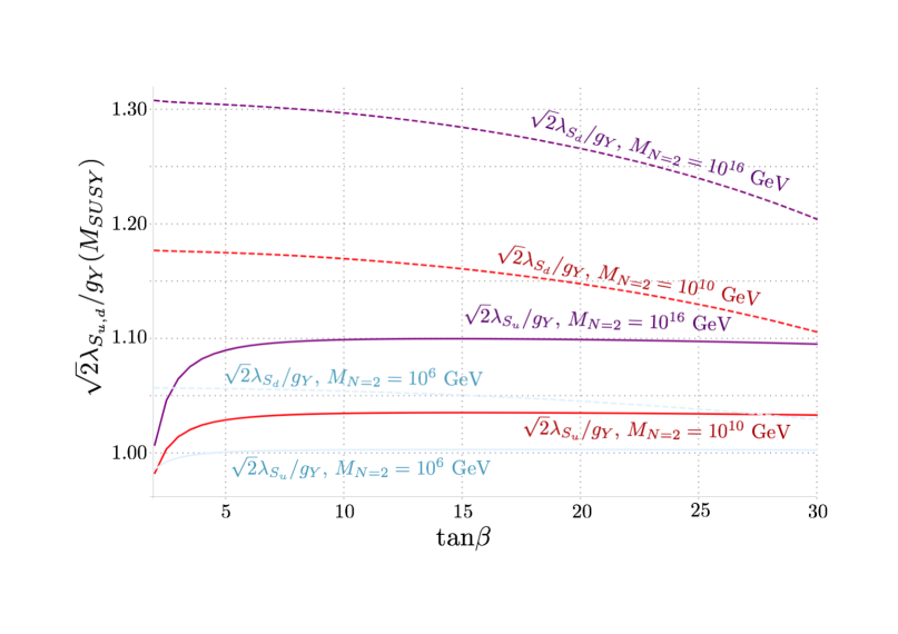
Refer to caption
Figure 9: Variations in the ratio 2λSu,d/gY2subscript𝜆subscript𝑆𝑢𝑑subscript𝑔𝑌\sqrt{2}\lambda_{S_{u,d}}/g_{Y} against tanβ𝛽\tan\beta at the MSUSYsubscript𝑀𝑆𝑈𝑆𝑌M_{SUSY} scale for N=2𝑁2N=2 scales 106,1010superscript106superscript101010^{6},10^{10} and 1016superscript101610^{16} GeV.
Refer to caption
Figure 10: Variations in the ratio 2λTu,d/g2subscript𝜆subscript𝑇𝑢𝑑𝑔\sqrt{2}\lambda_{T_{u,d}}/g against tanβ𝛽\tan\beta at the MSUSYsubscript𝑀𝑆𝑈𝑆𝑌M_{SUSY} scale for N=2𝑁2N=2 scales 106,1010superscript106superscript101010^{6},10^{10} and 1016superscript101610^{16} GeV.

The ratios in figures (9, 10) are taken with a common MSUSYsubscript𝑀𝑆𝑈𝑆𝑌M_{SUSY} scale of 101010 TeV, while the associated value of mhsubscript𝑚m_{h} is unconstrained. MΣsubscript𝑀ΣM_{\Sigma} is kept fixed - in figures (9, 10) chosen as MΣ=10MSUSYsubscript𝑀Σ10subscript𝑀𝑆𝑈𝑆𝑌M_{\Sigma}=10\,M_{SUSY}. Here the modulus of the ratio is plotted, since the λSdsubscript𝜆subscript𝑆𝑑\lambda_{S_{d}} ratio is negative to respect the N=2𝑁2N=2 supersymmetry relations. As expected, the model is closest to the alignment limit when the N=2𝑁2N=2 scale is closer to the MSUSYsubscript𝑀𝑆𝑈𝑆𝑌M_{SUSY} scale. It can be seen that the Higgs mass is boosted to a greater extent by the down-type couplings than the up-type, where the ratio 2λTd/g2subscript𝜆subscript𝑇𝑑𝑔\sqrt{2}\lambda_{T_{d}}/g has the largest effect, especially for higher values of N=2𝑁2N=2 scale.

Refer to caption
Figure 11: vZ1(MSUSY)𝑣subscript𝑍1subscript𝑀𝑆𝑈𝑆𝑌v\sqrt{Z_{1}(M_{SUSY})} against tanβ𝛽\tan\beta for N=2𝑁2N=2 scales 106superscript10610^{6} and 1016superscript101610^{16} GeV, corresponding to the “tree-level” value of mhsubscript𝑚m_{h} before running down in low-energy effective theory.

Figure 11 shows the “tree-level” Higgs mass against tanβ𝛽\tan\beta before running down from MSUSYsubscript𝑀𝑆𝑈𝑆𝑌M_{SUSY} (where the value of the Higgs mass calculated at mtsubscript𝑚𝑡m_{t} matches the experimental value). For the lowest values of MN=2subscript𝑀𝑁2M_{N=2} and MΣsubscript𝑀ΣM_{\Sigma} plotted, vZ1(MSUSY)𝑣subscript𝑍1subscript𝑀𝑆𝑈𝑆𝑌v\sqrt{Z_{1}(M_{SUSY})} is approximately MZsubscript𝑀𝑍M_{Z}, and where the former increase, so does the boost to the Higgs mass. This boost grows substantially for the simultaneously highest values of MN=2subscript𝑀𝑁2M_{N=2} and MΣsubscript𝑀ΣM_{\Sigma}, owing to the large (almost non-perturbative) λTsubscript𝜆𝑇\lambda_{T} couplings. While not shown here, it should be noted that even for MN=2=1010subscript𝑀𝑁2superscript1010M_{N=2}=10^{10} GeV and MΣ=100MSUSYsubscript𝑀Σ100subscript𝑀𝑆𝑈𝑆𝑌M_{\Sigma}=100\,M_{SUSY}, vZ1(MSUSY)𝑣subscript𝑍1subscript𝑀𝑆𝑈𝑆𝑌v\sqrt{Z_{1}(M_{SUSY})} replicates almost identical behaviour to the red curve for MN=2=1016subscript𝑀𝑁2superscript1016M_{N=2}=10^{16} GeV and MΣ=5MSUSYsubscript𝑀Σ5subscript𝑀𝑆𝑈𝑆𝑌M_{\Sigma}=5\,M_{SUSY} shown here.

6.1.3 Running from MSUSYQmtsubscript𝑀𝑆𝑈𝑆𝑌𝑄subscript𝑚𝑡M_{SUSY}\rightarrow Q\rightarrow m_{t}

Refer to caption
Figure 12: Z6(Q)subscript𝑍6𝑄Z_{6}(Q) against tanβ𝛽\tan\beta for a Higgs mass of 125125125 GeV at mtsubscript𝑚𝑡m_{t}, for values of MΣsubscript𝑀ΣM_{\Sigma} = 5, 100 MSUSYsubscript𝑀𝑆𝑈𝑆𝑌M_{SUSY} and MN=2=106subscript𝑀𝑁2superscript106M_{N=2}=10^{6} and 1016superscript101610^{16} GeV.

Figure 12 shows little deviation in the results for Z6(Q)subscript𝑍6𝑄Z_{6}(Q), regardless of MΣsubscript𝑀ΣM_{\Sigma} and MN=2subscript𝑀𝑁2M_{N=2}. Indeed, as anticipated above, the results are almost indistinguishable from the MSSM case, since the adjoint scalars in the MRSSM never give a large boost to the quartic couplings even for the extreme cases we have taken. Exceptionally, the couplings in the case of very heavy scalars and very high MN=2subscript𝑀𝑁2M_{N=2} are considerably enhanced and deviate from the N=2𝑁2N=2 relations, making the alignment in this case just marginally worse. While the adjoint scalars give only a very small boost to the Higgs mass, on the other hand it is enough to cause noticeable effects in the predicted MSUSYsubscript𝑀𝑆𝑈𝑆𝑌M_{SUSY} scale, shown in figure 13, because of the logarithmic nature of the contributions from other SUSY states.
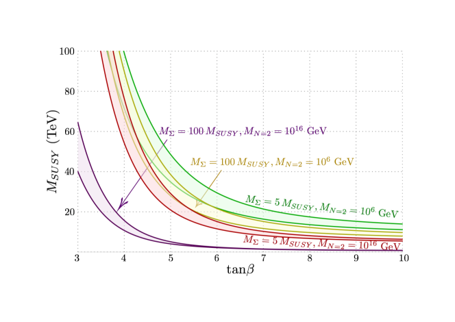
Refer to caption
Figure 13: MSUSYsubscript𝑀𝑆𝑈𝑆𝑌M_{SUSY} against tanβ𝛽\tan\beta for a Higgs mass of 125125125 GeV at mtsubscript𝑚𝑡m_{t} and where Q=600𝑄600Q=600 GeV, plotted for values of MΣsubscript𝑀ΣM_{\Sigma} = 5, 100 MSUSYsubscript𝑀𝑆𝑈𝑆𝑌M_{SUSY} and MN=2=106subscript𝑀𝑁2superscript106M_{N=2}=10^{6} and 1016superscript101610^{16} GeV.

Figure 13 shows the values of MSUSYsubscript𝑀𝑆𝑈𝑆𝑌M_{SUSY} against tanβ𝛽\tan\beta over the parameter scan producing a Higgs mass corresponding to mh=125±0.5subscript𝑚plus-or-minus1250.5m_{h}=125\pm 0.5 GeV: this margin is reflected in the enclosed transparent area666The variation of 0.50.50.5 GeV is, however, not to imply the total error (which is hard to estimate, but should be comparable to this value although it may be smaller for large values of MSUSYsubscript𝑀𝑆𝑈𝑆𝑌M_{SUSY}) but to give an indication of the sensitivity of the results on the final Higgs mass value.. For tanβ<4𝛽4\tan\beta<4, MSUSYsubscript𝑀𝑆𝑈𝑆𝑌M_{SUSY} is required to be, at the very least, 20 TeV for the highest values of MN=2subscript𝑀𝑁2M_{N=2} and very heavy MΣsubscript𝑀ΣM_{\Sigma}, and is closer to 100similar-toabsent100\sim 100 TeV for lower values. MSUSYsubscript𝑀𝑆𝑈𝑆𝑌M_{SUSY} stabilises around tanβ=10𝛽10\tan\beta=10 for all values of MΣsubscript𝑀ΣM_{\Sigma} and MN=2subscript𝑀𝑁2M_{N=2}, where at this point MSUSYsubscript𝑀𝑆𝑈𝑆𝑌M_{SUSY} can be as low as several hundred GeV for MN=2=1016subscript𝑀𝑁2superscript1016M_{N=2}=10^{16} and very heavy scalars. In this final extreme case (which is of course excluded experimentally, but we give as an indication of the possible effects) the logarithms being resummed in the RGEs become smaller, it is possible that any neglected threshold effects could make a significant difference and the results become unreliable, but we leave this additional analysis to future work.

7 Conclusions

We have considered the the consequences for the simplest realisation of Dirac gaugino models when we impose N=2𝑁2N=2 supersymmetric boundary conditions for the Higgs/gauge sector at some energy scale. We found that the model naturally realises alignment in the Higgs mass matrix, and that surprisingly this is preserved even by quantum corrections. Even more interestingly, the departure from N=2𝑁2N=2 relations due to running of the couplings actually leads to both an enhanced Higgs mass (and thus lower SUSY scale/more natural model) and also improved alignment when we take the effects of the squarks into account.

We have provided the most accurate calculation to date for the SUSY scale for a Dirac gaugino model by employing the effective field theory approach, with one-loop boundary conditions at the high scale and two loops at the THDM scale. This leads to the prediction that the scale of coloured superpartners should be above 333 TeV (when we allow a very high scale for the breaking of the approximate N=2𝑁2N=2 SUSY) but across most of the parameter space it is below 101010 TeV. While this is not encouraging for the detection of stops/gluinos at the LHC, this is well within the reach of a future 100100100 TeV collider. On the other hand, the LHC or a future e+esuperscript𝑒superscript𝑒e^{+}e^{-} collider should be able to explore the electroweak sector of the model, including the Higgs sector and the electroweakinos (if they are light).

There are many possible avenues for future work: improving the accuracy of the matching at MSUSYsubscript𝑀SUSYM_{\rm SUSY} (as noted recently, matching at two-loop order is often necessary for accuracy of the loop expansion to include all non-logarithmic corrections [100], although in this class of models as we have discussed all of the missing corrections are believed to be small) and including the effects of the electroweakinos in the matching at one loop, so that we can consider the model with mDYmD2MSUSYsimilar-tosubscript𝑚𝐷𝑌subscript𝑚𝐷2similar-tosubscript𝑀SUSYm_{DY}\sim m_{D2}\sim M_{\rm SUSY}; also with the full set of thresholds we could perform an estimate of the error in the calculation (which, again, should already be small – see e.g. the estimates for the MSSM case in [101]); or including the effects of possible R-symmetry violating terms. On the other hand, it would also be interesting to more fully explore the consequences for different Dirac gaugino models, such as the MRSSM, where we have only performed a preliminary analysis.


Acknowledgments

We are grateful to P. Slavich for many helpful discussions and comments on the manuscript. S. W. thanks J. Harz for help at the very early stage of the project. We acknowledge the support of the European Research Council (ERC) under the Advanced Grant Higgs@LHC (ERC-2012-ADG20120216-321133) and the Agence Nationale de Recherche under grant ANR-15-CE31-0002 “HiggsAutomator”. This work is also supported by the Labex “Institut Lagrange de Paris” (ANR-11-IDEX-0004-02, ANR-10-LABX-63)).

Appendix A THDM with light electroweakinos

The limit that we are interested in has the electroweakinos much lighter than the singlet and triplet scalars; in order to avoid washing out the tree-level Higgs quartic coupling and generating a large contribution to ρ𝜌\rho they should be light. At energies below the stop/sbottom masses, then, we have an effective theory of the two-Higgs doublet model augmented by light electroweakinos. This looks a little like Split supersymmetry or the scenario of [102] (which considered a split scenario with both Higgs doublets light), except that our electroweakinos have Dirac masses and our gluino is heavy; here are therefore new Yukawa couplings between the Higgs doublets ΦisubscriptΦ𝑖\Phi_{i}, the left and right bino B~isubscript~𝐵𝑖\tilde{B}_{i} and wino W~iasubscriptsuperscript~𝑊𝑎𝑖\tilde{W}^{a}_{i} for i=1,2𝑖12i=1,2, and the higgsinos h~u,dsubscript~𝑢𝑑\tilde{h}_{u,d}:

12[g~1uijΦiB~jh~u+g~2uijΦiW~jaσah~u+g~1dijΦiB~jh~d+g~2dijΦiW~jaσah~d+h.c.].\displaystyle\mathcal{L}\supset-\frac{1}{\sqrt{2}}\bigg{[}\tilde{g}_{1u}^{ij}\Phi_{i}^{*}\tilde{B}_{j}\tilde{h}_{u}+\tilde{g}_{2u}^{ij}\Phi_{i}^{*}\tilde{W}_{j}^{a}\sigma^{a}\tilde{h}_{u}+\tilde{g}_{1d}^{ij}\Phi_{i}\tilde{B}_{j}\tilde{h}_{d}+\tilde{g}_{2d}^{ij}\Phi_{i}\tilde{W}_{j}^{a}\sigma^{a}\tilde{h}_{d}+h.c.\bigg{]}. (A.1)

This gives neutral and charged fermion mass matrices

χ0=(MB012vkg1dki12vkg1uki0MW12vkg2dki12vkg2uki12vkg1dki12vkg2dki0μ12vkg1uki12vkg2ukiμ0),χ±=(MW12vkg2uki12vkg2dkiμ)formulae-sequencesubscriptsuperscript𝜒0subscript𝑀𝐵012subscript𝑣𝑘superscriptsubscript𝑔1𝑑𝑘𝑖12subscript𝑣𝑘superscriptsubscript𝑔1𝑢𝑘𝑖0subscript𝑀𝑊12subscript𝑣𝑘superscriptsubscript𝑔2𝑑𝑘𝑖12subscript𝑣𝑘superscriptsubscript𝑔2𝑢𝑘𝑖12subscript𝑣𝑘superscriptsubscript𝑔1𝑑𝑘𝑖12subscript𝑣𝑘superscriptsubscript𝑔2𝑑𝑘𝑖0𝜇12subscript𝑣𝑘superscriptsubscript𝑔1𝑢𝑘𝑖12subscript𝑣𝑘superscriptsubscript𝑔2𝑢𝑘𝑖𝜇0subscriptsuperscript𝜒plus-or-minussubscript𝑀𝑊12subscript𝑣𝑘superscriptsubscript𝑔2𝑢𝑘𝑖12subscript𝑣𝑘superscriptsubscript𝑔2𝑑𝑘𝑖𝜇\displaystyle\mathcal{M}_{\chi^{0}}=\left(\begin{array}[]{cccc}M_{B}&0&-\frac{1}{2}v_{k}g_{1d}^{ki}&\frac{1}{2}v_{k}g_{1u}^{ki}\\ 0&M_{W}&-\frac{1}{2}v_{k}g_{2d}^{ki}&-\frac{1}{2}v_{k}g_{2u}^{ki}\\ -\frac{1}{2}v_{k}g_{1d}^{ki}&-\frac{1}{2}v_{k}g_{2d}^{ki}&0&-\mu\\ \frac{1}{2}v_{k}g_{1u}^{ki}&-\frac{1}{2}v_{k}g_{2u}^{ki}&-\mu&0\end{array}\right),\qquad\mathcal{M}_{\chi^{\pm}}=\left(\begin{array}[]{cc}M_{W}&\frac{1}{\sqrt{2}}v_{k}g_{2u}^{ki}\\ -\frac{1}{\sqrt{2}}v_{k}g_{2d}^{ki}&\mu\end{array}\right) (A.8)

where the bases are χ0=(B~1,B~2,W~10,W~20,h~d0,h~u0)superscript𝜒0subscript~𝐵1subscript~𝐵2subscriptsuperscript~𝑊01subscriptsuperscript~𝑊02superscriptsubscript~𝑑0superscriptsubscript~𝑢0\chi^{0}=(\tilde{B}_{1},\tilde{B}_{2},\tilde{W}^{0}_{1},\tilde{W}^{0}_{2},\tilde{h}_{d}^{0},\tilde{h}_{u}^{0}) and the charged mass terms are (W~i,hd)χ±(W~i+hu+)subscriptsuperscript~𝑊𝑖superscriptsubscript𝑑subscriptsuperscript𝜒plus-or-minussubscriptsuperscript~𝑊𝑖superscriptsubscript𝑢\mathcal{L}\supset-(\tilde{W}^{-}_{i},h_{d}^{-})\mathcal{M}_{\chi^{\pm}}\left(\begin{array}[]{c}\tilde{W}^{+}_{i}\\ h_{u}^{+}\end{array}\right). Note that MB,MWsubscript𝑀𝐵subscript𝑀𝑊M_{B},M_{W} are 2×2222\times 2 matrices.

At the SUSY scale, we match the above to the corresponding couplings in the Dirac gaugino theory:

DGabsentsuperscript𝐷𝐺\displaystyle\mathcal{L}^{DG}\supset gY2HuB~1h~ug22HuW~1aσah~u+gY2HdB~1h~dg22HdW~1aσah~dsubscript𝑔𝑌2superscriptsubscript𝐻𝑢subscript~𝐵1subscript~𝑢subscript𝑔22superscriptsubscript𝐻𝑢superscriptsubscript~𝑊1𝑎superscript𝜎𝑎subscript~𝑢subscript𝑔𝑌2superscriptsubscript𝐻𝑑subscript~𝐵1subscript~𝑑subscript𝑔22superscriptsubscript𝐻𝑑superscriptsubscript~𝑊1𝑎superscript𝜎𝑎subscript~𝑑\displaystyle-\frac{g_{Y}}{\sqrt{2}}H_{u}^{*}\tilde{B}_{1}\tilde{h}_{u}-\frac{g_{2}}{\sqrt{2}}H_{u}^{*}\tilde{W}_{1}^{a}\sigma^{a}\tilde{h}_{u}+\frac{g_{Y}}{\sqrt{2}}H_{d}^{*}\tilde{B}_{1}\tilde{h}_{d}-\frac{g_{2}}{\sqrt{2}}H_{d}^{*}\tilde{W}_{1}^{a}\sigma^{a}\tilde{h}_{d}
λSHuB~2h~dλSh~uB~2HdλTHdW~2aσah~uλTh~dW~2aσaHu+h.c.formulae-sequencesubscript𝜆𝑆subscript𝐻𝑢subscript~𝐵2subscript~𝑑subscript𝜆𝑆subscript~𝑢subscript~𝐵2subscript𝐻𝑑subscript𝜆𝑇subscript𝐻𝑑superscriptsubscript~𝑊2𝑎superscript𝜎𝑎subscript~𝑢subscript𝜆𝑇subscript~𝑑superscriptsubscript~𝑊2𝑎superscript𝜎𝑎subscript𝐻𝑢𝑐\displaystyle-\lambda_{S}H_{u}\cdot\tilde{B}_{2}\tilde{h}_{d}-\lambda_{S}\tilde{h}_{u}\cdot\tilde{B}_{2}H_{d}-\lambda_{T}H_{d}\cdot\tilde{W}_{2}^{a}\sigma^{a}\tilde{h}_{u}-\lambda_{T}\tilde{h}_{d}\cdot\tilde{W}_{2}^{a}\sigma^{a}H_{u}+h.c. (A.9)

We choose to make the definition

Φ2=Hu,Φ1i=ϵij(Hdj)(Hd0Hd)=(Φ10(Φ1+))formulae-sequencesubscriptΦ2subscript𝐻𝑢superscriptsubscriptΦ1𝑖subscriptitalic-ϵ𝑖𝑗superscriptsuperscriptsubscript𝐻𝑑𝑗superscriptsubscript𝐻𝑑0superscriptsubscript𝐻𝑑superscriptsubscriptΦ10superscriptsuperscriptsubscriptΦ1\displaystyle\Phi_{2}=H_{u},\qquad\Phi_{1}^{i}=-\epsilon_{ij}(H_{d}^{j})^{*}\leftrightarrow\left(\begin{array}[]{c}H_{d}^{0}\\ H_{d}^{-}\end{array}\right)=\left(\begin{array}[]{c}\Phi_{1}^{0}\\ -(\Phi_{1}^{+})^{*}\end{array}\right) (A.14)

meaning HuHdΦ1Φ2subscript𝐻𝑢subscript𝐻𝑑superscriptsubscriptΦ1subscriptΦ2H_{u}\cdot H_{d}\leftrightarrow-\Phi_{1}^{\dagger}\Phi_{2}, which leads to the identifications

g1d11=0,g1d21=2λS,g1u11=2λS,g1u21=0formulae-sequencesuperscriptsubscript𝑔1𝑑110formulae-sequencesuperscriptsubscript𝑔1𝑑212subscript𝜆𝑆formulae-sequencesuperscriptsubscript𝑔1𝑢112subscript𝜆𝑆superscriptsubscript𝑔1𝑢210\displaystyle g_{1d}^{11}=0,\qquad g_{1d}^{21}=\sqrt{2}\lambda_{S},\qquad g_{1u}^{11}=-\sqrt{2}\lambda_{S},\qquad g_{1u}^{21}=0 (A.15)
g1d12=gY,g1d22=0,g1u12=0,g1u22=gYformulae-sequencesuperscriptsubscript𝑔1𝑑12subscript𝑔𝑌formulae-sequencesuperscriptsubscript𝑔1𝑑220formulae-sequencesuperscriptsubscript𝑔1𝑢120superscriptsubscript𝑔1𝑢22subscript𝑔𝑌\displaystyle g_{1d}^{12}=g_{Y},\qquad g_{1d}^{22}=0,\qquad g_{1u}^{12}=0,\qquad g_{1u}^{22}=g_{Y} (A.16)
g2d11=0,g2d21=2λT,g2u11=2λT,g2u21=0formulae-sequencesuperscriptsubscript𝑔2𝑑110formulae-sequencesuperscriptsubscript𝑔2𝑑212subscript𝜆𝑇formulae-sequencesuperscriptsubscript𝑔2𝑢112subscript𝜆𝑇superscriptsubscript𝑔2𝑢210\displaystyle g_{2d}^{11}=0,\qquad g_{2d}^{21}=\sqrt{2}\lambda_{T},\qquad g_{2u}^{11}=\sqrt{2}\lambda_{T},\qquad g_{2u}^{21}=0 (A.17)
g2d12=g2,g2d22=0,g2u12=0,g2u22=g2.formulae-sequencesuperscriptsubscript𝑔2𝑑12subscript𝑔2formulae-sequencesuperscriptsubscript𝑔2𝑑220formulae-sequencesuperscriptsubscript𝑔2𝑢120superscriptsubscript𝑔2𝑢22subscript𝑔2\displaystyle g_{2d}^{12}=-g_{2},\qquad g_{2d}^{22}=0,\qquad g_{2u}^{12}=0,\qquad g_{2u}^{22}=g_{2}. (A.18)

These are, however, given in terms of the DR¯¯DR\overline{\mathrm{DR}} parameters: making the conversion to MS¯¯MS\overline{\mathrm{MS}} we find

(g~1u,dij)MS¯=subscriptsuperscriptsubscript~𝑔1𝑢𝑑𝑖𝑗¯MSabsent\displaystyle(\tilde{g}_{1u,d}^{ij})_{\overline{\mathrm{MS}}}= (g~1u,dij)DR¯[114gY232π234g2232π2]subscriptsuperscriptsubscript~𝑔1𝑢𝑑𝑖𝑗¯DRdelimited-[]114subscriptsuperscript𝑔2𝑌32superscript𝜋234subscriptsuperscript𝑔2232superscript𝜋2\displaystyle(\tilde{g}_{1u,d}^{ij})_{\overline{\mathrm{DR}}}\bigg{[}1-\frac{1}{4}\frac{g^{2}_{Y}}{32\pi^{2}}-\frac{3}{4}\frac{g^{2}_{2}}{32\pi^{2}}\bigg{]}
(g~2u,dij)MS¯=subscriptsuperscriptsubscript~𝑔2𝑢𝑑𝑖𝑗¯MSabsent\displaystyle(\tilde{g}_{2u,d}^{ij})_{\overline{\mathrm{MS}}}= (g~2u,dij)DR¯[114gY232π2+54g2232π2].subscriptsuperscriptsubscript~𝑔2𝑢𝑑𝑖𝑗¯DRdelimited-[]114subscriptsuperscript𝑔2𝑌32superscript𝜋254subscriptsuperscript𝑔2232superscript𝜋2\displaystyle(\tilde{g}_{2u,d}^{ij})_{\overline{\mathrm{DR}}}\bigg{[}1-\frac{1}{4}\frac{g^{2}_{Y}}{32\pi^{2}}+\frac{5}{4}\frac{g^{2}_{2}}{32\pi^{2}}\bigg{]}. (A.19)

Appendix B Threshold corrections

In this section we give the one-loop threshold corrections to the couplings in our theory. Throughout we use the definitions

κ𝜅absent\displaystyle\kappa\equiv 116π2116superscript𝜋2\displaystyle\frac{1}{16\pi^{2}}
log¯x¯𝑥absent\displaystyle\overline{\log}\ x\equiv logxμ2𝑥superscript𝜇2\displaystyle\log\frac{x}{\mu^{2}}
PSS(x,y)subscript𝑃𝑆𝑆𝑥𝑦absent\displaystyle P_{SS}(x,y)\equiv xlog¯xylog¯yxy1,𝑥¯𝑥𝑦¯𝑦𝑥𝑦1\displaystyle\frac{x\overline{\log}x-y\overline{\log}y}{x-y}-1, (B.1)

where μ𝜇\mu is the renormalisation scale at which the quantities are evaluated.

B.1 Conversion from MS¯¯MS\overline{\mathrm{MS}} to DR¯¯DR\overline{\mathrm{DR}}

The conversion of the gauge couplings from the MS¯¯MS\overline{\mathrm{MS}} to DR¯¯DR\overline{\mathrm{DR}} renormalisation scheme is given by

(gY)MS¯=subscriptsubscript𝑔𝑌¯MSabsent\displaystyle(g_{Y})_{\overline{\rm MS}}= (gY)DR¯subscriptsubscript𝑔𝑌¯DR\displaystyle(g_{Y})_{\overline{\rm DR}}
(g2)MS¯=subscriptsubscript𝑔2¯MSabsent\displaystyle(g_{2})_{\overline{\rm MS}}= (g2)DR¯[1κg223]subscriptsubscript𝑔2¯DRdelimited-[]1𝜅subscriptsuperscript𝑔223\displaystyle(g_{2})_{\overline{\rm DR}}\bigg{[}1-\frac{\kappa g^{2}_{2}}{3}\bigg{]}
(g3)MS¯=subscriptsubscript𝑔3¯MSabsent\displaystyle(g_{3})_{\overline{\rm MS}}= (g3)DR¯[1κg322].subscriptsubscript𝑔3¯DRdelimited-[]1𝜅subscriptsuperscript𝑔232\displaystyle(g_{3})_{\overline{\rm DR}}\bigg{[}1-\frac{\kappa g^{2}_{3}}{2}\bigg{]}. (B.2)

For the Yukawa couplings, we retain only the strong gauge coupling dependence:

yMS¯t,bsimilar-to-or-equalssubscriptsuperscript𝑦𝑡𝑏¯MSabsent\displaystyle y^{t,b}_{\overline{\rm MS}}\simeq yDR¯t,b(1+43κg32).subscriptsuperscript𝑦𝑡𝑏¯DR143𝜅subscriptsuperscript𝑔23\displaystyle y^{t,b}_{\overline{\rm DR}}\bigg{(}1+\frac{4}{3}\kappa g^{2}_{3}\bigg{)}. (B.3)

For the Higgs quartic couplings, we define

λiMS¯=superscriptsubscript𝜆𝑖¯MSabsent\displaystyle\lambda_{i}^{\overline{\mathrm{MS}}}= λiDR¯+δλisuperscriptsubscript𝜆𝑖¯DR𝛿subscript𝜆𝑖\displaystyle\lambda_{i}^{\overline{\mathrm{DR}}}+\delta\lambda_{i} (B.4)

and then

δλ1=δλ2=𝛿subscript𝜆1𝛿subscript𝜆2absent\displaystyle\delta\lambda_{1}=\delta\lambda_{2}= κ4(gY4+3g24+gY2g22)𝜅4superscriptsubscript𝑔𝑌43superscriptsubscript𝑔24superscriptsubscript𝑔𝑌2superscriptsubscript𝑔22\displaystyle-\frac{\kappa}{4}\bigg{(}g_{Y}^{4}+3g_{2}^{4}+g_{Y}^{2}g_{2}^{2}\bigg{)}
δλ3=𝛿subscript𝜆3absent\displaystyle\delta\lambda_{3}= κ4(gY4+3g242gY2g22)𝜅4superscriptsubscript𝑔𝑌43superscriptsubscript𝑔242superscriptsubscript𝑔𝑌2superscriptsubscript𝑔22\displaystyle-\frac{\kappa}{4}\bigg{(}g_{Y}^{4}+3g_{2}^{4}-2g_{Y}^{2}g_{2}^{2}\bigg{)}
δλ4=𝛿subscript𝜆4absent\displaystyle\delta\lambda_{4}= κgY2g22.𝜅superscriptsubscript𝑔𝑌2superscriptsubscript𝑔22\displaystyle-\kappa g_{Y}^{2}g_{2}^{2}. (B.5)

If we express the quartic couplings in terms of the MS¯¯MS\overline{\mathrm{MS}} gauge couplings at tree level, then we have a further shift from the shift to g2subscript𝑔2g_{2} of +κ6g24𝜅6superscriptsubscript𝑔24+\frac{\kappa}{6}g_{2}^{4} for λ1,2subscript𝜆12\lambda_{1,2} and κ6g24𝜅6superscriptsubscript𝑔24-\frac{\kappa}{6}g_{2}^{4} for λ3subscript𝜆3\lambda_{3}.

B.2 Squark contributions

B.2.1 Matching at the SUSY scale

In the limit that we take in the body of the paper, all of the threshold corrections coming from squarks vanish at the matching scale. However, to extend the results of [103, 87] to our model, we have computed the corrections coming from stops, sbottoms and staus to the quartic couplings allowing non-zero squark trilinears and μ𝜇\mu. They are given by

δλi𝛿subscript𝜆𝑖absent\displaystyle\delta\lambda_{i}\equiv δth(1)λi+δΦ(1)λi,superscriptsubscript𝛿th1subscript𝜆𝑖superscriptsubscript𝛿Φ1subscript𝜆𝑖\displaystyle\delta_{\rm th}^{(1)}\lambda_{i}+\delta_{\Phi}^{(1)}\lambda_{i}, (B.6)

where the δth(1)λisuperscriptsubscript𝛿th1subscript𝜆𝑖\delta_{\rm th}^{(1)}\lambda_{i} contributions are those from bubble, triangle and box diagrams and are unchanged from the MSSM case given in [103, 87], while the δΦ(1)λisuperscriptsubscript𝛿Φ1subscript𝜆𝑖\delta_{\Phi}^{(1)}\lambda_{i} are the wavefunction corrections that are modified for our model:

κ1δΦ(1)λ1=superscript𝜅1superscriptsubscript𝛿Φ1subscript𝜆1absent\displaystyle\kappa^{-1}\delta_{\Phi}^{(1)}\lambda_{1}= g22+gY212MS2(3Ab2+3yt2μ2+Aτ2)superscriptsubscript𝑔22superscriptsubscript𝑔𝑌212superscriptsubscript𝑀𝑆23superscriptsubscript𝐴𝑏23superscriptsubscript𝑦𝑡2superscript𝜇2superscriptsubscript𝐴𝜏2\displaystyle-\frac{g_{2}^{2}+g_{Y}^{2}}{12M_{S}^{2}}(3A_{b}^{2}+3y_{t}^{2}\mu^{2}+A_{\tau}^{2})
κ1δΦ(1)λ2=superscript𝜅1superscriptsubscript𝛿Φ1subscript𝜆2absent\displaystyle\kappa^{-1}\delta_{\Phi}^{(1)}\lambda_{2}= g22+gY212MS2(3At2+3yb2μ2+μ2yτ2)superscriptsubscript𝑔22superscriptsubscript𝑔𝑌212superscriptsubscript𝑀𝑆23superscriptsubscript𝐴𝑡23superscriptsubscript𝑦𝑏2superscript𝜇2superscript𝜇2superscriptsubscript𝑦𝜏2\displaystyle-\frac{g_{2}^{2}+g_{Y}^{2}}{12M_{S}^{2}}(3A_{t}^{2}+3y_{b}^{2}\mu^{2}+\mu^{2}y_{\tau}^{2})
κ1δΦ(1)λ3=superscript𝜅1superscriptsubscript𝛿Φ1subscript𝜆3absent\displaystyle\kappa^{-1}\delta_{\Phi}^{(1)}\lambda_{3}= g22gY2+8λT224MS2(3At2+3Ab2+3(yb2+yt2)μ2+Aτ2+yτ2μ2)superscriptsubscript𝑔22superscriptsubscript𝑔𝑌28superscriptsubscript𝜆𝑇224superscriptsubscript𝑀𝑆23superscriptsubscript𝐴𝑡23superscriptsubscript𝐴𝑏23superscriptsubscript𝑦𝑏2superscriptsubscript𝑦𝑡2superscript𝜇2superscriptsubscript𝐴𝜏2superscriptsubscript𝑦𝜏2superscript𝜇2\displaystyle-\frac{g_{2}^{2}-g_{Y}^{2}+8\lambda_{T}^{2}}{24M_{S}^{2}}(3A_{t}^{2}+3A_{b}^{2}+3(y_{b}^{2}+y_{t}^{2})\mu^{2}+A_{\tau}^{2}+y_{\tau}^{2}\mu^{2})
κ1δΦ(1)λ4=superscript𝜅1superscriptsubscript𝛿Φ1subscript𝜆4absent\displaystyle\kappa^{-1}\delta_{\Phi}^{(1)}\lambda_{4}= g222λS2+2λT212MS2(3At2+3Ab2+3(yb2+yt2)μ2+Aτ2+yτ2μ2)superscriptsubscript𝑔222superscriptsubscript𝜆𝑆22superscriptsubscript𝜆𝑇212superscriptsubscript𝑀𝑆23superscriptsubscript𝐴𝑡23superscriptsubscript𝐴𝑏23superscriptsubscript𝑦𝑏2superscriptsubscript𝑦𝑡2superscript𝜇2superscriptsubscript𝐴𝜏2superscriptsubscript𝑦𝜏2superscript𝜇2\displaystyle\frac{g_{2}^{2}-2\lambda_{S}^{2}+2\lambda_{T}^{2}}{12M_{S}^{2}}(3A_{t}^{2}+3A_{b}^{2}+3(y_{b}^{2}+y_{t}^{2})\mu^{2}+A_{\tau}^{2}+y_{\tau}^{2}\mu^{2})
κ1δΦ(1)λ5=superscript𝜅1superscriptsubscript𝛿Φ1subscript𝜆5absent\displaystyle\kappa^{-1}\delta_{\Phi}^{(1)}\lambda_{5}= 00\displaystyle 0
κ1δΦ(1)λ6=superscript𝜅1superscriptsubscript𝛿Φ1subscript𝜆6absent\displaystyle\kappa^{-1}\delta_{\Phi}^{(1)}\lambda_{6}= λS2+λT212MS2μ(3Atyt+3Abyb+Aτyτ)superscriptsubscript𝜆𝑆2superscriptsubscript𝜆𝑇212superscriptsubscript𝑀𝑆2𝜇3subscript𝐴𝑡subscript𝑦𝑡3subscript𝐴𝑏subscript𝑦𝑏subscript𝐴𝜏subscript𝑦𝜏\displaystyle\frac{\lambda_{S}^{2}+\lambda_{T}^{2}}{12M_{S}^{2}}\mu(3A_{t}y_{t}+3A_{b}y_{b}+A_{\tau}y_{\tau})
κ1δΦ(1)λ7=superscript𝜅1superscriptsubscript𝛿Φ1subscript𝜆7absent\displaystyle\kappa^{-1}\delta_{\Phi}^{(1)}\lambda_{7}= κ1δΦ(1)λ6.superscript𝜅1superscriptsubscript𝛿Φ1subscript𝜆6\displaystyle\kappa^{-1}\delta_{\Phi}^{(1)}\lambda_{6}. (B.7)

B.2.2 Matching at a general scale

If the squarks are not degenerate or we integrate them out at a scale other than a common SUSY scale, then in our limit we have

κ1δλ1=superscript𝜅1𝛿subscript𝜆1absent\displaystyle\kappa^{-1}\delta\lambda_{1}= 124[(9g24+gY436g22yb212gY2yb2+72yb4)log¯mQ2+8gY4log¯mU2+2(gY26yb2)2log¯mD2]124delimited-[]9superscriptsubscript𝑔24superscriptsubscript𝑔𝑌436superscriptsubscript𝑔22superscriptsubscript𝑦𝑏212superscriptsubscript𝑔𝑌2superscriptsubscript𝑦𝑏272superscriptsubscript𝑦𝑏4¯superscriptsubscript𝑚𝑄28superscriptsubscript𝑔𝑌4¯superscriptsubscript𝑚𝑈22superscriptsuperscriptsubscript𝑔𝑌26superscriptsubscript𝑦𝑏22¯superscriptsubscript𝑚𝐷2\displaystyle\frac{1}{24}\bigg{[}(9g_{2}^{4}+g_{Y}^{4}-36g_{2}^{2}y_{b}^{2}-12g_{Y}^{2}y_{b}^{2}+72y_{b}^{4})\overline{\log}m_{Q}^{2}+8g_{Y}^{4}\overline{\log}m_{U}^{2}+2(g_{Y}^{2}-6y_{b}^{2})^{2}\overline{\log}m_{D}^{2}\bigg{]}
+18[2(gY22yτ2)2log¯mE2+(g24+gY44g22yτ2+4gY2yτ2+8yτ4)log¯mL2]18delimited-[]2superscriptsuperscriptsubscript𝑔𝑌22superscriptsubscript𝑦𝜏22¯superscriptsubscript𝑚𝐸2superscriptsubscript𝑔24superscriptsubscript𝑔𝑌44superscriptsubscript𝑔22superscriptsubscript𝑦𝜏24superscriptsubscript𝑔𝑌2superscriptsubscript𝑦𝜏28superscriptsubscript𝑦𝜏4¯superscriptsubscript𝑚𝐿2\displaystyle+\frac{1}{8}\bigg{[}2(g_{Y}^{2}-2y_{\tau}^{2})^{2}\overline{\log}m_{E}^{2}+(g_{2}^{4}+g_{Y}^{4}-4g_{2}^{2}y_{\tau}^{2}+4g_{Y}^{2}y_{\tau}^{2}+8y_{\tau}^{4})\overline{\log}m_{L}^{2}\bigg{]}
κ1δλ2=superscript𝜅1𝛿subscript𝜆2absent\displaystyle\kappa^{-1}\delta\lambda_{2}= 124[(9g24+gY436g22yt212gY2yt2+72yt4)log¯mQ2+2gY4log¯mD2+8(gY23yt2)2log¯mU2]124delimited-[]9superscriptsubscript𝑔24superscriptsubscript𝑔𝑌436superscriptsubscript𝑔22superscriptsubscript𝑦𝑡212superscriptsubscript𝑔𝑌2superscriptsubscript𝑦𝑡272superscriptsubscript𝑦𝑡4¯superscriptsubscript𝑚𝑄22superscriptsubscript𝑔𝑌4¯superscriptsubscript𝑚𝐷28superscriptsuperscriptsubscript𝑔𝑌23superscriptsubscript𝑦𝑡22¯superscriptsubscript𝑚𝑈2\displaystyle\frac{1}{24}\bigg{[}(9g_{2}^{4}+g_{Y}^{4}-36g_{2}^{2}y_{t}^{2}-12g_{Y}^{2}y_{t}^{2}+72y_{t}^{4})\overline{\log}m_{Q}^{2}+2g_{Y}^{4}\overline{\log}m_{D}^{2}+8(g_{Y}^{2}-3y_{t}^{2})^{2}\overline{\log}m_{U}^{2}\bigg{]}
+18[2gY4log¯mE2+(g24+gY4)log¯mL2]18delimited-[]2superscriptsubscript𝑔𝑌4¯superscriptsubscript𝑚𝐸2superscriptsubscript𝑔24superscriptsubscript𝑔𝑌4¯superscriptsubscript𝑚𝐿2\displaystyle+\frac{1}{8}\bigg{[}2g_{Y}^{4}\overline{\log}m_{E}^{2}+(g_{2}^{4}+g_{Y}^{4})\overline{\log}m_{L}^{2}\bigg{]}
κ1δλ3=superscript𝜅1𝛿subscript𝜆3absent\displaystyle\kappa^{-1}\delta\lambda_{3}= 3yb2yt2PSS(mD2,mU2)3superscriptsubscript𝑦𝑏2superscriptsubscript𝑦𝑡2subscript𝑃𝑆𝑆superscriptsubscript𝑚𝐷2superscriptsubscript𝑚𝑈2\displaystyle 3y_{b}^{2}y_{t}^{2}P_{SS}(m_{D}^{2},m_{U}^{2})
+124[(9g24gY4+72yt2yb2+6gY2(yb2yt2)18g22(yb2+yt2))log¯mQ2\displaystyle+\frac{1}{24}\bigg{[}(9g_{2}^{4}-g_{Y}^{4}+72y_{t}^{2}y_{b}^{2}+6g_{Y}^{2}(y_{b}^{2}-y_{t}^{2})-18g_{2}^{2}(y_{b}^{2}+y_{t}^{2}))\overline{\log}m_{Q}^{2}
2gY2(gY26yb2)log¯mD28gY2(gY23yt2)log¯mU2]\displaystyle-2g_{Y}^{2}(g_{Y}^{2}-6y_{b}^{2})\overline{\log}m_{D}^{2}-8g_{Y}^{2}(g_{Y}^{2}-3y_{t}^{2})\overline{\log}m_{U}^{2}\bigg{]}
+18[2gY2(gY22yτ2)log¯mE2+(g22+gY2)(g22gY22yτ2)log¯mL2]18delimited-[]2superscriptsubscript𝑔𝑌2superscriptsubscript𝑔𝑌22superscriptsubscript𝑦𝜏2¯superscriptsubscript𝑚𝐸2superscriptsubscript𝑔22superscriptsubscript𝑔𝑌2superscriptsubscript𝑔22superscriptsubscript𝑔𝑌22superscriptsubscript𝑦𝜏2¯superscriptsubscript𝑚𝐿2\displaystyle+\frac{1}{8}\bigg{[}-2g_{Y}^{2}(g_{Y}^{2}-2y_{\tau}^{2})\overline{\log}m_{E}^{2}+(g_{2}^{2}+g_{Y}^{2})(g_{2}^{2}-g_{Y}^{2}-2y_{\tau}^{2})\overline{\log}m_{L}^{2}\bigg{]}
κ1δλ4=superscript𝜅1𝛿subscript𝜆4absent\displaystyle\kappa^{-1}\delta\lambda_{4}= 3yb2yt2PSS(mD2,mU2)34[(g222yb2)(g222yt2)]log¯mQ23superscriptsubscript𝑦𝑏2superscriptsubscript𝑦𝑡2subscript𝑃𝑆𝑆superscriptsubscript𝑚𝐷2superscriptsubscript𝑚𝑈234delimited-[]superscriptsubscript𝑔222superscriptsubscript𝑦𝑏2superscriptsubscript𝑔222superscriptsubscript𝑦𝑡2¯superscriptsubscript𝑚𝑄2\displaystyle-3y_{b}^{2}y_{t}^{2}P_{SS}(m_{D}^{2},m_{U}^{2})-\frac{3}{4}\bigg{[}(g_{2}^{2}-2y_{b}^{2})(g_{2}^{2}-2y_{t}^{2})\bigg{]}\overline{\log}m_{Q}^{2}
14g22(g222yτ2)log¯mL2.14superscriptsubscript𝑔22superscriptsubscript𝑔222superscriptsubscript𝑦𝜏2¯superscriptsubscript𝑚𝐿2\displaystyle-\frac{1}{4}g_{2}^{2}(g_{2}^{2}-2y_{\tau}^{2})\overline{\log}m_{L}^{2}. (B.8)

If we consider all squarks to be at a common SUSY scale MSsubscript𝑀𝑆M_{S}, then these simplify to

κ1δλ1=superscript𝜅1𝛿subscript𝜆1absent\displaystyle\kappa^{-1}\delta\lambda_{1}= 16log¯MS2[3g24+5gY43(g22+gY2)(3yb2+yτ2)+12(3yb4+yτ4)]16¯superscriptsubscript𝑀𝑆2delimited-[]3superscriptsubscript𝑔245superscriptsubscript𝑔𝑌43superscriptsubscript𝑔22superscriptsubscript𝑔𝑌23superscriptsubscript𝑦𝑏2superscriptsubscript𝑦𝜏2123superscriptsubscript𝑦𝑏4superscriptsubscript𝑦𝜏4\displaystyle\frac{1}{6}\overline{\log}M_{S}^{2}\bigg{[}3g_{2}^{4}+5g_{Y}^{4}-3(g_{2}^{2}+g_{Y}^{2})(3y_{b}^{2}+y_{\tau}^{2})+12(3y_{b}^{4}+y_{\tau}^{4})\bigg{]}
κ1δλ2=superscript𝜅1𝛿subscript𝜆2absent\displaystyle\kappa^{-1}\delta\lambda_{2}= 16log¯MS2[3g24+5gY49g22yt215gY2yt2+36yt2]16¯superscriptsubscript𝑀𝑆2delimited-[]3superscriptsubscript𝑔245superscriptsubscript𝑔𝑌49superscriptsubscript𝑔22superscriptsubscript𝑦𝑡215superscriptsubscript𝑔𝑌2superscriptsubscript𝑦𝑡236superscriptsubscript𝑦𝑡2\displaystyle\frac{1}{6}\overline{\log}M_{S}^{2}\bigg{[}3g_{2}^{4}+5g_{Y}^{4}-9g_{2}^{2}y_{t}^{2}-15g_{Y}^{2}y_{t}^{2}+36y_{t}^{2}\bigg{]}
κ1δλ3=superscript𝜅1𝛿subscript𝜆3absent\displaystyle\kappa^{-1}\delta\lambda_{3}= 112log¯MS2[6g2410gY4+72yb2yt23(g22+gY2)(3yb2+3yt2+yτ2))]\displaystyle\frac{1}{12}\overline{\log}M_{S}^{2}\bigg{[}6g_{2}^{4}-10g_{Y}^{4}+72y_{b}^{2}y_{t}^{2}-3(g_{2}^{2}+g_{Y}^{2})(3y_{b}^{2}+3y_{t}^{2}+y_{\tau}^{2}))\bigg{]}
κ1δλ4=superscript𝜅1𝛿subscript𝜆4absent\displaystyle\kappa^{-1}\delta\lambda_{4}= 12log¯MS2[2g2412yb2yt2+g22(3yb2+3yt2+yτ2))]\displaystyle\frac{1}{2}\overline{\log}M_{S}^{2}\bigg{[}-2g_{2}^{4}-12y_{b}^{2}y_{t}^{2}+g_{2}^{2}(3y_{b}^{2}+3y_{t}^{2}+y_{\tau}^{2}))\bigg{]}
κ1(δλ3+δλ4)=superscript𝜅1𝛿subscript𝜆3𝛿subscript𝜆4absent\displaystyle\kappa^{-1}(\delta\lambda_{3}+\delta\lambda_{4})= 112log¯MS2[6g2410gY4+3(g22gY2)(3yb2+3yt2+yτ2))].\displaystyle\frac{1}{12}\overline{\log}M_{S}^{2}\bigg{[}-6g_{2}^{4}-10g_{Y}^{4}+3(g_{2}^{2}-g_{Y}^{2})(3y_{b}^{2}+3y_{t}^{2}+y_{\tau}^{2}))\bigg{]}. (B.9)

B.3 Contributions from the S,T𝑆𝑇S,T scalars

Here we present the contributions to the quartic couplings coming from the adjoint scalars S,T𝑆𝑇S,T, in the limit mDY,mD2mS,mT,BS,BTformulae-sequencemuch-less-thansubscript𝑚𝐷𝑌subscript𝑚𝐷2subscript𝑚𝑆subscript𝑚𝑇subscript𝐵𝑆subscript𝐵𝑇m_{DY},m_{D2}\ll m_{S},m_{T},B_{S},B_{T} and assuming no CP-violation. The scalars have masses

mSR2=superscriptsubscript𝑚𝑆𝑅2absent\displaystyle m_{SR}^{2}= mS2+BS+4mDY2mS2+BS,mSI2=mS2BSformulae-sequencesimilar-to-or-equalssuperscriptsubscript𝑚𝑆2subscript𝐵𝑆4superscriptsubscript𝑚𝐷𝑌2superscriptsubscript𝑚𝑆2subscript𝐵𝑆superscriptsubscript𝑚𝑆𝐼2superscriptsubscript𝑚𝑆2subscript𝐵𝑆\displaystyle m_{S}^{2}+B_{S}+4m_{DY}^{2}\simeq m_{S}^{2}+B_{S},\qquad m_{SI}^{2}=m_{S}^{2}-B_{S} (B.10)
mTP2=superscriptsubscript𝑚𝑇𝑃2absent\displaystyle m_{TP}^{2}= mT2+BT+4mD22mT2+BT,mTM2=mT2BT.formulae-sequencesimilar-to-or-equalssuperscriptsubscript𝑚𝑇2subscript𝐵𝑇4superscriptsubscript𝑚𝐷22superscriptsubscript𝑚𝑇2subscript𝐵𝑇superscriptsubscript𝑚𝑇𝑀2superscriptsubscript𝑚𝑇2subscript𝐵𝑇\displaystyle m_{T}^{2}+B_{T}+4m_{D2}^{2}\simeq m_{T}^{2}+B_{T},\qquad m_{TM}^{2}=m_{T}^{2}-B_{T}. (B.11)

The loop corrections to the quartic couplings are:

δλ1=δλ2=116π212[\displaystyle\delta\lambda_{1}=\delta\lambda_{2}=\frac{1}{16\pi^{2}}\frac{1}{2}\bigg{[} λS4logmSR2mSI2μ4+3λT4logmTP2mTM2μ4+(g222λT2)2PSS(mTM2,mTP2)superscriptsubscript𝜆𝑆4superscriptsubscript𝑚𝑆𝑅2superscriptsubscript𝑚𝑆𝐼2superscript𝜇43superscriptsubscript𝜆𝑇4superscriptsubscript𝑚𝑇𝑃2superscriptsubscript𝑚𝑇𝑀2superscript𝜇4superscriptsuperscriptsubscript𝑔222superscriptsubscript𝜆𝑇22subscript𝑃𝑆𝑆superscriptsubscript𝑚𝑇𝑀2superscriptsubscript𝑚𝑇𝑃2\displaystyle\lambda_{S}^{4}\log\frac{m_{SR}^{2}m_{SI}^{2}}{\mu^{4}}+3\lambda_{T}^{4}\log\frac{m_{TP}^{2}m_{TM}^{2}}{\mu^{4}}+(g_{2}^{2}-2\lambda_{T}^{2})^{2}P_{SS}(m_{TM}^{2},m_{TP}^{2})
+2λS2λT2(PSS(mSR2,mTP2)+PSS(mSI2,mTM2))]\displaystyle+2\lambda_{S}^{2}\lambda_{T}^{2}\bigg{(}P_{SS}(m_{SR}^{2},m_{TP}^{2})+P_{SS}(m_{SI}^{2},m_{TM}^{2})\bigg{)}\bigg{]}
δλ3=116π212[\displaystyle\delta\lambda_{3}=\frac{1}{16\pi^{2}}\frac{1}{2}\bigg{[} λS4logmSR2mSI2μ4+3λT4logmTP2mTM2μ4+(g222λT2)2PSS(mTM2,mTP2)superscriptsubscript𝜆𝑆4superscriptsubscript𝑚𝑆𝑅2superscriptsubscript𝑚𝑆𝐼2superscript𝜇43superscriptsubscript𝜆𝑇4superscriptsubscript𝑚𝑇𝑃2superscriptsubscript𝑚𝑇𝑀2superscript𝜇4superscriptsuperscriptsubscript𝑔222superscriptsubscript𝜆𝑇22subscript𝑃𝑆𝑆superscriptsubscript𝑚𝑇𝑀2superscriptsubscript𝑚𝑇𝑃2\displaystyle\lambda_{S}^{4}\log\frac{m_{SR}^{2}m_{SI}^{2}}{\mu^{4}}+3\lambda_{T}^{4}\log\frac{m_{TP}^{2}m_{TM}^{2}}{\mu^{4}}+(g_{2}^{2}-2\lambda_{T}^{2})^{2}P_{SS}(m_{TM}^{2},m_{TP}^{2})
2λS2λT2(PSS(mSR2,mTP2)+PSS(mSI2,mTM2))]\displaystyle-2\lambda_{S}^{2}\lambda_{T}^{2}\bigg{(}P_{SS}(m_{SR}^{2},m_{TP}^{2})+P_{SS}(m_{SI}^{2},m_{TM}^{2})\bigg{)}\bigg{]}
δλ4=116π2[\displaystyle\delta\lambda_{4}=\frac{1}{16\pi^{2}}\bigg{[} (g222λT2)2PSS(mTM2,mTP2)superscriptsuperscriptsubscript𝑔222superscriptsubscript𝜆𝑇22subscript𝑃𝑆𝑆superscriptsubscript𝑚𝑇𝑀2superscriptsubscript𝑚𝑇𝑃2\displaystyle-(g_{2}^{2}-2\lambda_{T}^{2})^{2}P_{SS}(m_{TM}^{2},m_{TP}^{2})
+2λS2λT2(PSS(mSR2,mTP2)+PSS(mSI2,mTM2))].\displaystyle+2\lambda_{S}^{2}\lambda_{T}^{2}\bigg{(}P_{SS}(m_{SR}^{2},m_{TP}^{2})+P_{SS}(m_{SI}^{2},m_{TM}^{2})\bigg{)}\bigg{]}. (B.12)

These results update those previously given in the literature by including the electroweak contributions.

Appendix C One-loop RGEs

For our numerical study we use two-loop RGEs throughout, as generated by SARAH. They are too long to put into print; however, for illustration we provide here the one-loop expressions for the low-energy theory of the THDM with electroweakinos, after making the simplification that:

  • Only third generation Yukawa couplings are included.

  • No CP-violation, hence all couplings real.

  • Once we respect the matching conditions (A.15-A.18), the beta functions for the couplings that are zero at the supersmmetry scale are zero along the flow, and hence we set the couplings g1d11superscriptsubscript𝑔1𝑑11g_{1d}^{11}, g1u21superscriptsubscript𝑔1𝑢21g_{1u}^{21}, g1d22superscriptsubscript𝑔1𝑑22g_{1d}^{22}, g1u12superscriptsubscript𝑔1𝑢12g_{1u}^{12}, g2d11superscriptsubscript𝑔2𝑑11g_{2d}^{11}, g2u21superscriptsubscript𝑔2𝑢21g_{2u}^{21}, g2d22superscriptsubscript𝑔2𝑑22g_{2d}^{22}, g2u12superscriptsubscript𝑔2𝑢12g_{2u}^{12} to zero.

We then define

dxdlogμκβx(1)+κ2βx(2)+𝑑𝑥𝑑𝜇𝜅superscriptsubscript𝛽𝑥1superscript𝜅2superscriptsubscript𝛽𝑥2\displaystyle\frac{dx}{d\log\mu}\equiv\kappa\beta_{x}^{(1)}+\kappa^{2}\beta_{x}^{(2)}+... (C.1)

and give below the RGEs for the dimensionless quantities in the theory.

C.1 Gauge couplings

βgY(1)=233gY3βg2(1)=13g23βg3(1)=7g33superscriptsubscript𝛽subscript𝑔𝑌1233superscriptsubscript𝑔𝑌3superscriptsubscript𝛽subscript𝑔2113superscriptsubscript𝑔23superscriptsubscript𝛽subscript𝑔317superscriptsubscript𝑔33\displaystyle\begin{aligned} \hfil\displaystyle\begin{split}\qquad\qquad\beta_{g_{Y}}^{(1)}&=\frac{23}{3}g_{Y}^{3}\end{split}\\[5.69054pt] \hfil\displaystyle\begin{split}\qquad\qquad\beta_{g_{2}}^{(1)}&=\frac{1}{3}g_{2}^{3}\end{split}\\[5.69054pt] \hfil\displaystyle\begin{split}\qquad\qquad\beta_{g_{3}}^{(1)}&=-7g_{3}^{3}\end{split}\end{aligned} (C.2)

C.2 Yukawa couplings

βyb(1)=subscriptsuperscript𝛽1subscript𝑦𝑏absent\displaystyle\beta^{(1)}_{y_{b}}= 112yb(27g2296g325gY2+54yb2+6yt2+12yτ2+6(g1d12)2+6(g1u11)2+18(g2d12)2+18(g2u11)2)112subscript𝑦𝑏27superscriptsubscript𝑔2296superscriptsubscript𝑔325superscriptsubscript𝑔𝑌254superscriptsubscript𝑦𝑏26superscriptsubscript𝑦𝑡212superscriptsubscript𝑦𝜏26superscriptsuperscriptsubscript𝑔1𝑑1226superscriptsuperscriptsubscript𝑔1𝑢11218superscriptsuperscriptsubscript𝑔2𝑑12218superscriptsuperscriptsubscript𝑔2𝑢112\displaystyle\frac{1}{12}y_{b}(-27g_{2}^{2}-96g_{3}^{2}-5g_{Y}^{2}+54y_{b}^{2}+6y_{t}^{2}+12y_{\tau}^{2}+6(g_{1d}^{12})^{2}+6(g_{1u}^{11})^{2}+18(g_{2d}^{12})^{2}+18(g_{2u}^{11})^{2}) (C.3)
βyt(1)=subscriptsuperscript𝛽1subscript𝑦𝑡absent\displaystyle\beta^{(1)}_{y_{t}}= 112yt(27g2296g3217gY2+6yb2+54yt2+6(g1d21)2+6(g1u22)2+18(g2d21)2+18(g2u22)2)112subscript𝑦𝑡27superscriptsubscript𝑔2296superscriptsubscript𝑔3217superscriptsubscript𝑔𝑌26superscriptsubscript𝑦𝑏254superscriptsubscript𝑦𝑡26superscriptsuperscriptsubscript𝑔1𝑑2126superscriptsuperscriptsubscript𝑔1𝑢22218superscriptsuperscriptsubscript𝑔2𝑑21218superscriptsuperscriptsubscript𝑔2𝑢222\displaystyle\frac{1}{12}y_{t}(-27g_{2}^{2}-96g_{3}^{2}-17g_{Y}^{2}+6y_{b}^{2}+54y_{t}^{2}+6(g_{1d}^{21})^{2}+6(g_{1u}^{22})^{2}+18(g_{2d}^{21})^{2}+18(g_{2u}^{22})^{2})
βyτ(1)=subscriptsuperscript𝛽1subscript𝑦𝜏absent\displaystyle\beta^{(1)}_{y_{\tau}}= 14yτ(9g2215gY2+2(6yb2+5yτ2+(g1d12)2+(g1u11)2+3(g2d12)2+3(g2u11)2))14subscript𝑦𝜏9superscriptsubscript𝑔2215superscriptsubscript𝑔𝑌226superscriptsubscript𝑦𝑏25superscriptsubscript𝑦𝜏2superscriptsuperscriptsubscript𝑔1𝑑122superscriptsuperscriptsubscript𝑔1𝑢1123superscriptsuperscriptsubscript𝑔2𝑑1223superscriptsuperscriptsubscript𝑔2𝑢112\displaystyle\frac{1}{4}y_{\tau}(-9g_{2}^{2}-15g_{Y}^{2}+2(6y_{b}^{2}+5y_{\tau}^{2}+(g_{1d}^{12})^{2}+(g_{1u}^{11})^{2}+3(g_{2d}^{12})^{2}+3(g_{2u}^{11})^{2}))
βg1d12(1)=subscriptsuperscript𝛽1superscriptsubscript𝑔1𝑑12absent\displaystyle\beta^{(1)}_{g_{1d}^{12}}= 120(10g1u22(2g1u11g1d21+g1d12g1u22+6g2u11g2d21)\displaystyle\frac{1}{20}(10g_{1u}^{22}(2g_{1u}^{11}g_{1d}^{21}+g_{1d}^{12}g_{1u}^{22}+6g_{2u}^{11}g_{2d}^{21})
+5g1d12(9g223gY2+12yb2+4yτ2+5(g1d12)2+2(g1u11)2+9(g2d12)2+6(g2u11)2+(g1d21)2+3(g2d21)2))\displaystyle+5g_{1d}^{12}(-9g_{2}^{2}-3g_{Y}^{2}+12y_{b}^{2}+4y_{\tau}^{2}+5(g_{1d}^{12})^{2}+2(g_{1u}^{11})^{2}+9(g_{2d}^{12})^{2}+6(g_{2u}^{11})^{2}+(g_{1d}^{21})^{2}+3(g_{2d}^{21})^{2}))
βg1u11(1)=subscriptsuperscript𝛽1superscriptsubscript𝑔1𝑢11absent\displaystyle\beta^{(1)}_{g_{1u}^{11}}= 120(10g1d21(g1u11g1d21+2g1d12g1u22+6g2d12g2u22)\displaystyle\frac{1}{20}(10g_{1d}^{21}(g_{1u}^{11}g_{1d}^{21}+2g_{1d}^{12}g_{1u}^{22}+6g_{2d}^{12}g_{2u}^{22})
+5g1u11(9g223gY2+12yb2+4yτ2+2(g1d12)2+5(g1u11)2+6(g2d12)2+9(g2u11)2+(g1u22)2+3(g2u22)2))\displaystyle+5g_{1u}^{11}(-9g_{2}^{2}-3g_{Y}^{2}+12y_{b}^{2}+4y_{\tau}^{2}+2(g_{1d}^{12})^{2}+5(g_{1u}^{11})^{2}+6(g_{2d}^{12})^{2}+9(g_{2u}^{11})^{2}+(g_{1u}^{22})^{2}+3(g_{2u}^{22})^{2}))
βg2d12(1)=subscriptsuperscript𝛽1superscriptsubscript𝑔2𝑑12absent\displaystyle\beta^{(1)}_{g_{2d}^{12}}= 120(5g2d12(33g223gY2+12yb2+4yτ2+3(g1d12)2+2(g1u11)2+11(g2d12)2+6(g2u11)2+(g1d21)2+3(g2d21)2)\displaystyle\frac{1}{20}(5g_{2d}^{12}(-33g_{2}^{2}-3g_{Y}^{2}+12y_{b}^{2}+4y_{\tau}^{2}+3(g_{1d}^{12})^{2}+2(g_{1u}^{11})^{2}+11(g_{2d}^{12})^{2}+6(g_{2u}^{11})^{2}+(g_{1d}^{21})^{2}+3(g_{2d}^{21})^{2})
+10g2u22(2g1u11g1d212g2u11g2d21+g2d12g2u22))\displaystyle+10g_{2u}^{22}(2g_{1u}^{11}g_{1d}^{21}-2g_{2u}^{11}g_{2d}^{21}+g_{2d}^{12}g_{2u}^{22}))
βg2u11(1)=subscriptsuperscript𝛽1superscriptsubscript𝑔2𝑢11absent\displaystyle\beta^{(1)}_{g_{2u}^{11}}= 120(10g2d21(2g1d12g1u22+g2u11g2d212g2d12g2u22)\displaystyle\frac{1}{20}(10g_{2d}^{21}(2g_{1d}^{12}g_{1u}^{22}+g_{2u}^{11}g_{2d}^{21}-2g_{2d}^{12}g_{2u}^{22})
+5g2u11(33g223gY2+12yb2+4yτ2+2(g1d12)2+3(g1u11)2+6(g2d12)2+11(g2u11)2+(g1u22)2+3(g2u22)2))\displaystyle+5g_{2u}^{11}(-33g_{2}^{2}-3g_{Y}^{2}+12y_{b}^{2}+4y_{\tau}^{2}+2(g_{1d}^{12})^{2}+3(g_{1u}^{11})^{2}+6(g_{2d}^{12})^{2}+11(g_{2u}^{11})^{2}+(g_{1u}^{22})^{2}+3(g_{2u}^{22})^{2}))
βg1d21(1)=subscriptsuperscript𝛽1superscriptsubscript𝑔1𝑑21absent\displaystyle\beta^{(1)}_{g_{1d}^{21}}= 120(10g1u11(g1u11g1d21+2g1d12g1u22+6g2d12g2u22)\displaystyle\frac{1}{20}(10g_{1u}^{11}(g_{1u}^{11}g_{1d}^{21}+2g_{1d}^{12}g_{1u}^{22}+6g_{2d}^{12}g_{2u}^{22})
+5g1d21(9g223gY2+12yt2+(g1d12)2+3(g2d12)2+5(g1d21)2+2(g1u22)2+9(g2d21)2+6(g2u22)2))\displaystyle+5g_{1d}^{21}(-9g_{2}^{2}-3g_{Y}^{2}+12y_{t}^{2}+(g_{1d}^{12})^{2}+3(g_{2d}^{12})^{2}+5(g_{1d}^{21})^{2}+2(g_{1u}^{22})^{2}+9(g_{2d}^{21})^{2}+6(g_{2u}^{22})^{2}))
βg1u22(1)=subscriptsuperscript𝛽1superscriptsubscript𝑔1𝑢22absent\displaystyle\beta^{(1)}_{g_{1u}^{22}}= 14(2(g1d12)2g1u22+4g1d12(g1u11g1d21+3g2u11g2d21)\displaystyle\frac{1}{4}(2(g_{1d}^{12})^{2}g_{1u}^{22}+4g_{1d}^{12}(g_{1u}^{11}g_{1d}^{21}+3g_{2u}^{11}g_{2d}^{21})
+g1u22(9g223gY2+12yt2+(g1u11)2+3(g2u11)2+2(g1d21)2+5(g1u22)2+6(g2d21)2+9(g2u22)2))\displaystyle+g_{1u}^{22}(-9g_{2}^{2}-3g_{Y}^{2}+12y_{t}^{2}+(g_{1u}^{11})^{2}+3(g_{2u}^{11})^{2}+2(g_{1d}^{21})^{2}+5(g_{1u}^{22})^{2}+6(g_{2d}^{21})^{2}+9(g_{2u}^{22})^{2}))
βg2d21(1)=subscriptsuperscript𝛽1superscriptsubscript𝑔2𝑑21absent\displaystyle\beta^{(1)}_{g_{2d}^{21}}= 120(10g2u11(2g1d12g1u22+g2u11g2d212g2d12g2u22)\displaystyle\frac{1}{20}(10g_{2u}^{11}(2g_{1d}^{12}g_{1u}^{22}+g_{2u}^{11}g_{2d}^{21}-2g_{2d}^{12}g_{2u}^{22})
+5g2d21(33g223gY2+12yt2+(g1d12)2+3(g2d12)2+3(g1d21)2+2(g1u22)2+11(g2d21)2+6(g2u22)2))\displaystyle+5g_{2d}^{21}(-33g_{2}^{2}-3g_{Y}^{2}+12y_{t}^{2}+(g_{1d}^{12})^{2}+3(g_{2d}^{12})^{2}+3(g_{1d}^{21})^{2}+2(g_{1u}^{22})^{2}+11(g_{2d}^{21})^{2}+6(g_{2u}^{22})^{2}))
βg2u22(1)=subscriptsuperscript𝛽1superscriptsubscript𝑔2𝑢22absent\displaystyle\beta^{(1)}_{g_{2u}^{22}}= 14(4g1u11g2d12g1d214g2d12g2u11g2d21+(g1u11)2g2u22+2(g2d12)2g2u22\displaystyle\frac{1}{4}(4g_{1u}^{11}g_{2d}^{12}g_{1d}^{21}-4g_{2d}^{12}g_{2u}^{11}g_{2d}^{21}+(g_{1u}^{11})^{2}g_{2u}^{22}+2(g_{2d}^{12})^{2}g_{2u}^{22}
+g2u22(33g223gY2+12yt2+3(g2u11)2+2(g1d21)2+3(g1u22)2+6(g2d21)2+11(g2u22)2)).\displaystyle+g_{2u}^{22}(-33g_{2}^{2}-3g_{Y}^{2}+12y_{t}^{2}+3(g_{2u}^{11})^{2}+2(g_{1d}^{21})^{2}+3(g_{1u}^{22})^{2}+6(g_{2d}^{21})^{2}+11(g_{2u}^{22})^{2})).

C.3 Quartic scalar couplings

βλ1(1)=subscriptsuperscript𝛽1subscript𝜆1absent\displaystyle\beta^{(1)}_{\lambda_{1}}= 14(9g24+3gY4+6g22(gY26λ1)12gY2λ1)(12yb4+4yτ412yb2λ14yτ2λ112λ12\displaystyle\frac{1}{4}\bigg{(}9g_{2}^{4}+3g_{Y}^{4}+6g_{2}^{2}(g_{Y}^{2}-6\lambda_{1})-12g_{Y}^{2}\lambda_{1}\bigg{)}-\bigg{(}12y_{b}^{4}+4y_{\tau}^{4}-12y_{b}^{2}\lambda_{1}-4y_{\tau}^{2}\lambda_{1}-12\lambda_{1}^{2} (C.4)
4λ324λ3λ42λ422λ522λ1(g1d12)2+(g1d12)42λ1(g1u11)2+(g1u11)46λ1(g2d12)24superscriptsubscript𝜆324subscript𝜆3subscript𝜆42superscriptsubscript𝜆422superscriptsubscript𝜆522subscript𝜆1superscriptsuperscriptsubscript𝑔1𝑑122superscriptsuperscriptsubscript𝑔1𝑑1242subscript𝜆1superscriptsuperscriptsubscript𝑔1𝑢112superscriptsuperscriptsubscript𝑔1𝑢1146subscript𝜆1superscriptsuperscriptsubscript𝑔2𝑑122\displaystyle-4\lambda_{3}^{2}-4\lambda_{3}\lambda_{4}-2\lambda_{4}^{2}-2\lambda_{5}^{2}-2\lambda_{1}(g_{1d}^{12})^{2}+(g_{1d}^{12})^{4}-2\lambda_{1}(g_{1u}^{11})^{2}+(g_{1u}^{11})^{4}-6\lambda_{1}(g_{2d}^{12})^{2}
+2(g1d12)2(g2d12)2+5(g2d12)46λ1(g2u11)2+2(g1u11)2(g2u11)2+5(g2u11)4)\displaystyle+2(g_{1d}^{12})^{2}(g_{2d}^{12})^{2}+5(g_{2d}^{12})^{4}-6\lambda_{1}(g_{2u}^{11})^{2}+2(g_{1u}^{11})^{2}(g_{2u}^{11})^{2}+5(g_{2u}^{11})^{4}\bigg{)}
βλ2(1)=subscriptsuperscript𝛽1subscript𝜆2absent\displaystyle\beta^{(1)}_{\lambda_{2}}= 14(9g24+3gY4+6g22(gY26λ2)12gY2λ2)(12yt412yt2λ212λ224λ324λ3λ4\displaystyle\frac{1}{4}\bigg{(}9g_{2}^{4}+3g_{Y}^{4}+6g_{2}^{2}(g_{Y}^{2}-6\lambda_{2})-12g_{Y}^{2}\lambda_{2}\bigg{)}-\bigg{(}12y_{t}^{4}-12y_{t}^{2}\lambda_{2}-12\lambda_{2}^{2}-4\lambda_{3}^{2}-4\lambda_{3}\lambda_{4}
2λ422λ52+(g1d21)4+(g1u22)4+2(g1d21)2(g2d21)2+5(g2d21)4+2(g1u22)2(g2u22)2+5(g2u22)42superscriptsubscript𝜆422superscriptsubscript𝜆52superscriptsuperscriptsubscript𝑔1𝑑214superscriptsuperscriptsubscript𝑔1𝑢2242superscriptsuperscriptsubscript𝑔1𝑑212superscriptsuperscriptsubscript𝑔2𝑑2125superscriptsuperscriptsubscript𝑔2𝑑2142superscriptsuperscriptsubscript𝑔1𝑢222superscriptsuperscriptsubscript𝑔2𝑢2225superscriptsuperscriptsubscript𝑔2𝑢224\displaystyle-2\lambda_{4}^{2}-2\lambda_{5}^{2}+(g_{1d}^{21})^{4}+(g_{1u}^{22})^{4}+2(g_{1d}^{21})^{2}(g_{2d}^{21})^{2}+5(g_{2d}^{21})^{4}+2(g_{1u}^{22})^{2}(g_{2u}^{22})^{2}+5(g_{2u}^{22})^{4}
2λ2[(g1d21)2+(g1u22)2+3((g2d21)2+(g2u22)2)])\displaystyle-2\lambda_{2}\big{[}(g_{1d}^{21})^{2}+(g_{1u}^{22})^{2}+3((g_{2d}^{21})^{2}+(g_{2u}^{22})^{2})\big{]}\bigg{)}
βλ3(1)=subscriptsuperscript𝛽1subscript𝜆3absent\displaystyle\beta^{(1)}_{\lambda_{3}}= 94g2432g22gY2+34gY412yb2yt29g22λ33gY2λ3+6yb2λ3+6yt2λ3+2yτ2λ3+6λ1λ3+6λ2λ3+4λ3294superscriptsubscript𝑔2432superscriptsubscript𝑔22superscriptsubscript𝑔𝑌234superscriptsubscript𝑔𝑌412superscriptsubscript𝑦𝑏2superscriptsubscript𝑦𝑡29superscriptsubscript𝑔22subscript𝜆33superscriptsubscript𝑔𝑌2subscript𝜆36superscriptsubscript𝑦𝑏2subscript𝜆36superscriptsubscript𝑦𝑡2subscript𝜆32superscriptsubscript𝑦𝜏2subscript𝜆36subscript𝜆1subscript𝜆36subscript𝜆2subscript𝜆34superscriptsubscript𝜆32\displaystyle\frac{9}{4}g_{2}^{4}-\frac{3}{2}g_{2}^{2}g_{Y}^{2}+\frac{3}{4}g_{Y}^{4}-12y_{b}^{2}y_{t}^{2}-9g_{2}^{2}\lambda_{3}-3g_{Y}^{2}\lambda_{3}+6y_{b}^{2}\lambda_{3}+6y_{t}^{2}\lambda_{3}+2y_{\tau}^{2}\lambda_{3}+6\lambda_{1}\lambda_{3}+6\lambda_{2}\lambda_{3}+4\lambda_{3}^{2}
+2λ1λ4+2λ2λ4+2λ42+2λ52+3λ3(g2d12)2+3λ3(g2u11)2+λ3(g1d21)2(g1u11)2(g1d21)22(g2d12)2(g1d21)22subscript𝜆1subscript𝜆42subscript𝜆2subscript𝜆42superscriptsubscript𝜆422superscriptsubscript𝜆523subscript𝜆3superscriptsuperscriptsubscript𝑔2𝑑1223subscript𝜆3superscriptsuperscriptsubscript𝑔2𝑢112subscript𝜆3superscriptsuperscriptsubscript𝑔1𝑑212superscriptsuperscriptsubscript𝑔1𝑢112superscriptsuperscriptsubscript𝑔1𝑑2122superscriptsuperscriptsubscript𝑔2𝑑122superscriptsuperscriptsubscript𝑔1𝑑212\displaystyle+2\lambda_{1}\lambda_{4}+2\lambda_{2}\lambda_{4}+2\lambda_{4}^{2}+2\lambda_{5}^{2}+3\lambda_{3}(g_{2d}^{12})^{2}+3\lambda_{3}(g_{2u}^{11})^{2}+\lambda_{3}(g_{1d}^{21})^{2}-(g_{1u}^{11})^{2}(g_{1d}^{21})^{2}-2(g_{2d}^{12})^{2}(g_{1d}^{21})^{2}
+λ3(g1u22)2(g1d12)2(g1u22)22(g2u11)2(g1u22)2+2g1u11g2u11g1d21g2d214g1d12g2u11g1u22g2d21+3λ3(g2d21)24(g2d12)2(g2d21)2subscript𝜆3superscriptsuperscriptsubscript𝑔1𝑢222superscriptsuperscriptsubscript𝑔1𝑑122superscriptsuperscriptsubscript𝑔1𝑢2222superscriptsuperscriptsubscript𝑔2𝑢112superscriptsuperscriptsubscript𝑔1𝑢2222superscriptsubscript𝑔1𝑢11superscriptsubscript𝑔2𝑢11superscriptsubscript𝑔1𝑑21superscriptsubscript𝑔2𝑑214superscriptsubscript𝑔1𝑑12superscriptsubscript𝑔2𝑢11superscriptsubscript𝑔1𝑢22superscriptsubscript𝑔2𝑑213subscript𝜆3superscriptsuperscriptsubscript𝑔2𝑑2124superscriptsuperscriptsubscript𝑔2𝑑122superscriptsuperscriptsubscript𝑔2𝑑212\displaystyle+\lambda_{3}(g_{1u}^{22})^{2}-(g_{1d}^{12})^{2}(g_{1u}^{22})^{2}-2(g_{2u}^{11})^{2}(g_{1u}^{22})^{2}+2g_{1u}^{11}g_{2u}^{11}g_{1d}^{21}g_{2d}^{21}-4g_{1d}^{12}g_{2u}^{11}g_{1u}^{22}g_{2d}^{21}+3\lambda_{3}(g_{2d}^{21})^{2}-4(g_{2d}^{12})^{2}(g_{2d}^{21})^{2}
5(g2u11)2(g2d21)2+(g1d12)2(λ32(g2d21)2)4g1u11g2d12g1d21g2u22+2g1d12g2d12g1u22g2u22+8g2d12g2u11g2d21g2u225superscriptsuperscriptsubscript𝑔2𝑢112superscriptsuperscriptsubscript𝑔2𝑑212superscriptsuperscriptsubscript𝑔1𝑑122subscript𝜆32superscriptsuperscriptsubscript𝑔2𝑑2124superscriptsubscript𝑔1𝑢11superscriptsubscript𝑔2𝑑12superscriptsubscript𝑔1𝑑21superscriptsubscript𝑔2𝑢222superscriptsubscript𝑔1𝑑12superscriptsubscript𝑔2𝑑12superscriptsubscript𝑔1𝑢22superscriptsubscript𝑔2𝑢228superscriptsubscript𝑔2𝑑12superscriptsubscript𝑔2𝑢11superscriptsubscript𝑔2𝑑21superscriptsubscript𝑔2𝑢22\displaystyle-5(g_{2u}^{11})^{2}(g_{2d}^{21})^{2}+(g_{1d}^{12})^{2}(\lambda_{3}-2(g_{2d}^{21})^{2})-4g_{1u}^{11}g_{2d}^{12}g_{1d}^{21}g_{2u}^{22}+2g_{1d}^{12}g_{2d}^{12}g_{1u}^{22}g_{2u}^{22}+8g_{2d}^{12}g_{2u}^{11}g_{2d}^{21}g_{2u}^{22}
+3λ3(g2u22)25(g2d12)2(g2u22)24(g2u11)2(g2u22)2+(g1u11)2(λ32(g2u22)2)3subscript𝜆3superscriptsuperscriptsubscript𝑔2𝑢2225superscriptsuperscriptsubscript𝑔2𝑑122superscriptsuperscriptsubscript𝑔2𝑢2224superscriptsuperscriptsubscript𝑔2𝑢112superscriptsuperscriptsubscript𝑔2𝑢222superscriptsuperscriptsubscript𝑔1𝑢112subscript𝜆32superscriptsuperscriptsubscript𝑔2𝑢222\displaystyle+3\lambda_{3}(g_{2u}^{22})^{2}-5(g_{2d}^{12})^{2}(g_{2u}^{22})^{2}-4(g_{2u}^{11})^{2}(g_{2u}^{22})^{2}+(g_{1u}^{11})^{2}(\lambda_{3}-2(g_{2u}^{22})^{2})
βλ4(1)=subscriptsuperscript𝛽1subscript𝜆4absent\displaystyle\beta^{(1)}_{\lambda_{4}}= 3g22gY2+12yb2yt29g22λ43gY2λ4+6yb2λ4+6yt2λ4+2yτ2λ4+2λ1λ4+2λ2λ4+8λ3λ4+4λ42+8λ523superscriptsubscript𝑔22superscriptsubscript𝑔𝑌212superscriptsubscript𝑦𝑏2superscriptsubscript𝑦𝑡29superscriptsubscript𝑔22subscript𝜆43superscriptsubscript𝑔𝑌2subscript𝜆46superscriptsubscript𝑦𝑏2subscript𝜆46superscriptsubscript𝑦𝑡2subscript𝜆42superscriptsubscript𝑦𝜏2subscript𝜆42subscript𝜆1subscript𝜆42subscript𝜆2subscript𝜆48subscript𝜆3subscript𝜆44superscriptsubscript𝜆428superscriptsubscript𝜆52\displaystyle 3g_{2}^{2}g_{Y}^{2}+12y_{b}^{2}y_{t}^{2}-9g_{2}^{2}\lambda_{4}-3g_{Y}^{2}\lambda_{4}+6y_{b}^{2}\lambda_{4}+6y_{t}^{2}\lambda_{4}+2y_{\tau}^{2}\lambda_{4}+2\lambda_{1}\lambda_{4}+2\lambda_{2}\lambda_{4}+8\lambda_{3}\lambda_{4}+4\lambda_{4}^{2}+8\lambda_{5}^{2}
+3λ4(g2d12)2+3λ4(g2u11)2+λ4(g1d21)2+(g2d12)2(g1d21)22g1d12g1u11g1d21g1u22+λ4(g1u22)2+(g2u11)2(g1u22)23subscript𝜆4superscriptsuperscriptsubscript𝑔2𝑑1223subscript𝜆4superscriptsuperscriptsubscript𝑔2𝑢112subscript𝜆4superscriptsuperscriptsubscript𝑔1𝑑212superscriptsuperscriptsubscript𝑔2𝑑122superscriptsuperscriptsubscript𝑔1𝑑2122superscriptsubscript𝑔1𝑑12superscriptsubscript𝑔1𝑢11superscriptsubscript𝑔1𝑑21superscriptsubscript𝑔1𝑢22subscript𝜆4superscriptsuperscriptsubscript𝑔1𝑢222superscriptsuperscriptsubscript𝑔2𝑢112superscriptsuperscriptsubscript𝑔1𝑢222\displaystyle+3\lambda_{4}(g_{2d}^{12})^{2}+3\lambda_{4}(g_{2u}^{11})^{2}+\lambda_{4}(g_{1d}^{21})^{2}+(g_{2d}^{12})^{2}(g_{1d}^{21})^{2}-2g_{1d}^{12}g_{1u}^{11}g_{1d}^{21}g_{1u}^{22}+\lambda_{4}(g_{1u}^{22})^{2}+(g_{2u}^{11})^{2}(g_{1u}^{22})^{2}
4g1u11g2u11g1d21g2d21+2g1d12g2u11g1u22g2d21+3λ4(g2d21)2(g2d12)2(g2d21)2+4(g2u11)2(g2d21)24superscriptsubscript𝑔1𝑢11superscriptsubscript𝑔2𝑢11superscriptsubscript𝑔1𝑑21superscriptsubscript𝑔2𝑑212superscriptsubscript𝑔1𝑑12superscriptsubscript𝑔2𝑢11superscriptsubscript𝑔1𝑢22superscriptsubscript𝑔2𝑑213subscript𝜆4superscriptsuperscriptsubscript𝑔2𝑑212superscriptsuperscriptsubscript𝑔2𝑑122superscriptsuperscriptsubscript𝑔2𝑑2124superscriptsuperscriptsubscript𝑔2𝑢112superscriptsuperscriptsubscript𝑔2𝑑212\displaystyle-4g_{1u}^{11}g_{2u}^{11}g_{1d}^{21}g_{2d}^{21}+2g_{1d}^{12}g_{2u}^{11}g_{1u}^{22}g_{2d}^{21}+3\lambda_{4}(g_{2d}^{21})^{2}-(g_{2d}^{12})^{2}(g_{2d}^{21})^{2}+4(g_{2u}^{11})^{2}(g_{2d}^{21})^{2}
+(g1d12)2(λ4(g1d21)2+(g2d21)2)+2g1u11g2d12g1d21g2u224g1d12g2d12g1u22g2u2210g2d12g2u11g2d21g2u22superscriptsuperscriptsubscript𝑔1𝑑122subscript𝜆4superscriptsuperscriptsubscript𝑔1𝑑212superscriptsuperscriptsubscript𝑔2𝑑2122superscriptsubscript𝑔1𝑢11superscriptsubscript𝑔2𝑑12superscriptsubscript𝑔1𝑑21superscriptsubscript𝑔2𝑢224superscriptsubscript𝑔1𝑑12superscriptsubscript𝑔2𝑑12superscriptsubscript𝑔1𝑢22superscriptsubscript𝑔2𝑢2210superscriptsubscript𝑔2𝑑12superscriptsubscript𝑔2𝑢11superscriptsubscript𝑔2𝑑21superscriptsubscript𝑔2𝑢22\displaystyle+(g_{1d}^{12})^{2}(\lambda_{4}-(g_{1d}^{21})^{2}+(g_{2d}^{21})^{2})+2g_{1u}^{11}g_{2d}^{12}g_{1d}^{21}g_{2u}^{22}-4g_{1d}^{12}g_{2d}^{12}g_{1u}^{22}g_{2u}^{22}-10g_{2d}^{12}g_{2u}^{11}g_{2d}^{21}g_{2u}^{22}
+3λ4(g2u22)2+4(g2d12)2(g2u22)2(g2u11)2(g2u22)2+(g1u11)2(λ4(g1u22)2+(g2u22)2)3subscript𝜆4superscriptsuperscriptsubscript𝑔2𝑢2224superscriptsuperscriptsubscript𝑔2𝑑122superscriptsuperscriptsubscript𝑔2𝑢222superscriptsuperscriptsubscript𝑔2𝑢112superscriptsuperscriptsubscript𝑔2𝑢222superscriptsuperscriptsubscript𝑔1𝑢112subscript𝜆4superscriptsuperscriptsubscript𝑔1𝑢222superscriptsuperscriptsubscript𝑔2𝑢222\displaystyle+3\lambda_{4}(g_{2u}^{22})^{2}+4(g_{2d}^{12})^{2}(g_{2u}^{22})^{2}-(g_{2u}^{11})^{2}(g_{2u}^{22})^{2}+(g_{1u}^{11})^{2}(\lambda_{4}-(g_{1u}^{22})^{2}+(g_{2u}^{22})^{2})
βλ5(1)=subscriptsuperscript𝛽1subscript𝜆5absent\displaystyle\beta^{(1)}_{\lambda_{5}}= λ5(9g223gY2+6yb2+6yt2+2yτ2+2λ1+2λ2+8λ3+12λ4\displaystyle\lambda_{5}\bigg{(}-9g_{2}^{2}-3g_{Y}^{2}+6y_{b}^{2}+6y_{t}^{2}+2y_{\tau}^{2}+2\lambda_{1}+2\lambda_{2}+8\lambda_{3}+12\lambda_{4}
+(g1d12)2+(g1u11)2+3(g2d12)2+3(g2u11)2+(g1d21)2+(g1u22)2+3(g2d21)2+3(g2u22)2).\displaystyle+(g_{1d}^{12})^{2}+(g_{1u}^{11})^{2}+3(g_{2d}^{12})^{2}+3(g_{2u}^{11})^{2}+(g_{1d}^{21})^{2}+(g_{1u}^{22})^{2}+3(g_{2d}^{21})^{2}+3(g_{2u}^{22})^{2}\bigg{)}.

Appendix D MRSSM corrections

Here we collect the tree-level and leading one-loop threshold corrections to the THDM paramters in the MRSSM.

D.1 Tree-level

The tree-level λisubscript𝜆𝑖\lambda_{i} are given by

λ1=λ2=14(g22+gY2),λ3=14(g22gY2),λ4=12g22.formulae-sequencesubscript𝜆1subscript𝜆214superscriptsubscript𝑔22superscriptsubscript𝑔𝑌2formulae-sequencesubscript𝜆314superscriptsubscript𝑔22superscriptsubscript𝑔𝑌2subscript𝜆412superscriptsubscript𝑔22\displaystyle\lambda_{1}=\lambda_{2}=\frac{1}{4}(g_{2}^{2}+g_{Y}^{2}),\qquad\lambda_{3}=\frac{1}{4}(g_{2}^{2}-g_{Y}^{2}),\qquad\lambda_{4}=-\frac{1}{2}g_{2}^{2}. (D.1)

The shifts from integrating out the adjoint scalars give

δλ1=𝛿subscript𝜆1absent\displaystyle\delta\lambda_{1}= (gYmDY2λSdμd)2mSR2(g2mD2+2λTdμd)2mTP2superscriptsubscript𝑔𝑌subscript𝑚𝐷𝑌2subscript𝜆subscript𝑆𝑑subscript𝜇𝑑2superscriptsubscript𝑚𝑆𝑅2superscriptsubscript𝑔2subscript𝑚𝐷22subscript𝜆subscript𝑇𝑑subscript𝜇𝑑2superscriptsubscript𝑚𝑇𝑃2\displaystyle-\frac{(g_{Y}m_{DY}-\sqrt{2}\lambda_{S_{d}}\mu_{d})^{2}}{m_{SR}^{2}}-\frac{(g_{2}m_{D2}+\sqrt{2}\lambda_{T_{d}}\mu_{d})^{2}}{m_{TP}^{2}}
δλ2=𝛿subscript𝜆2absent\displaystyle\delta\lambda_{2}= (gYmDY+2λSuμu)2mSR2(g2mD2+2λTuμu)2mTP2superscriptsubscript𝑔𝑌subscript𝑚𝐷𝑌2subscript𝜆subscript𝑆𝑢subscript𝜇𝑢2superscriptsubscript𝑚𝑆𝑅2superscriptsubscript𝑔2subscript𝑚𝐷22subscript𝜆subscript𝑇𝑢subscript𝜇𝑢2superscriptsubscript𝑚𝑇𝑃2\displaystyle-\frac{(g_{Y}m_{DY}+\sqrt{2}\lambda_{S_{u}}\mu_{u})^{2}}{m_{SR}^{2}}-\frac{(g_{2}m_{D2}+\sqrt{2}\lambda_{T_{u}}\mu_{u})^{2}}{m_{TP}^{2}}
δλ3=𝛿subscript𝜆3absent\displaystyle\delta\lambda_{3}= AT2mTM2AT2mTP2superscriptsubscript𝐴𝑇2superscriptsubscript𝑚𝑇𝑀2superscriptsubscript𝐴𝑇2superscriptsubscript𝑚𝑇𝑃2\displaystyle-\frac{A_{T}^{2}}{m_{TM}^{2}}-\frac{A_{T}^{2}}{m_{TP}^{2}}
+(gYmDY2λSdμd)(gYmDY+2λSuμu)mSR2(g2mD2+2λTdμd)(g2mD2+2λTuμu)mTP2subscript𝑔𝑌subscript𝑚𝐷𝑌2subscript𝜆subscript𝑆𝑑subscript𝜇𝑑subscript𝑔𝑌subscript𝑚𝐷𝑌2subscript𝜆subscript𝑆𝑢subscript𝜇𝑢superscriptsubscript𝑚𝑆𝑅2subscript𝑔2subscript𝑚𝐷22subscript𝜆subscript𝑇𝑑subscript𝜇𝑑subscript𝑔2subscript𝑚𝐷22subscript𝜆subscript𝑇𝑢subscript𝜇𝑢superscriptsubscript𝑚𝑇𝑃2\displaystyle+\frac{(g_{Y}m_{DY}-\sqrt{2}\lambda_{S_{d}}\mu_{d})(g_{Y}m_{DY}+\sqrt{2}\lambda_{S_{u}}\mu_{u})}{m_{SR}^{2}}-\frac{(g_{2}m_{D2}+\sqrt{2}\lambda_{T_{d}}\mu_{d})(g_{2}m_{D2}+\sqrt{2}\lambda_{T_{u}}\mu_{u})}{m_{TP}^{2}}
δλ4=𝛿subscript𝜆4absent\displaystyle\delta\lambda_{4}= AS22mSI2AS22mSR2+AT22mTM2+AT22mTP2superscriptsubscript𝐴𝑆22superscriptsubscript𝑚𝑆𝐼2superscriptsubscript𝐴𝑆22superscriptsubscript𝑚𝑆𝑅2superscriptsubscript𝐴𝑇22superscriptsubscript𝑚𝑇𝑀2superscriptsubscript𝐴𝑇22superscriptsubscript𝑚𝑇𝑃2\displaystyle-\frac{A_{S}^{2}}{2m_{SI}^{2}}-\frac{A_{S}^{2}}{2m_{SR}^{2}}+\frac{A_{T}^{2}}{2m_{TM}^{2}}+\frac{A_{T}^{2}}{2m_{TP}^{2}}
+2(g2mD2+2λTdμd)(g2mD2+2λTuμu)mTP22subscript𝑔2subscript𝑚𝐷22subscript𝜆subscript𝑇𝑑subscript𝜇𝑑subscript𝑔2subscript𝑚𝐷22subscript𝜆subscript𝑇𝑢subscript𝜇𝑢superscriptsubscript𝑚𝑇𝑃2\displaystyle+2\frac{(g_{2}m_{D2}+\sqrt{2}\lambda_{T_{d}}\mu_{d})(g_{2}m_{D2}+\sqrt{2}\lambda_{T_{u}}\mu_{u})}{m_{TP}^{2}}
δλ5=𝛿subscript𝜆5absent\displaystyle\delta\lambda_{5}= AS22mSI2AS22mSR2+AT22mTM2AT22mTP2superscriptsubscript𝐴𝑆22superscriptsubscript𝑚𝑆𝐼2superscriptsubscript𝐴𝑆22superscriptsubscript𝑚𝑆𝑅2superscriptsubscript𝐴𝑇22superscriptsubscript𝑚𝑇𝑀2superscriptsubscript𝐴𝑇22superscriptsubscript𝑚𝑇𝑃2\displaystyle\frac{A_{S}^{2}}{2m_{SI}^{2}}-\frac{A_{S}^{2}}{2m_{SR}^{2}}+\frac{A_{T}^{2}}{2m_{TM}^{2}}-\frac{A_{T}^{2}}{2m_{TP}^{2}}
δλ6=𝛿subscript𝜆6absent\displaystyle\delta\lambda_{6}= AS(gYmDY+2λSdμd)2mSR2+AT(g2mD2+2λTdμd)2mTP2subscript𝐴𝑆subscript𝑔𝑌subscript𝑚𝐷𝑌2subscript𝜆subscript𝑆𝑑subscript𝜇𝑑2superscriptsubscript𝑚𝑆𝑅2subscript𝐴𝑇subscript𝑔2subscript𝑚𝐷22subscript𝜆subscript𝑇𝑑subscript𝜇𝑑2superscriptsubscript𝑚𝑇𝑃2\displaystyle\frac{A_{S}(-g_{Y}m_{DY}+\sqrt{2}\lambda_{S_{d}}\mu_{d})}{\sqrt{2}m_{SR}^{2}}+\frac{A_{T}(g_{2}m_{D2}+\sqrt{2}\lambda_{T_{d}}\mu_{d})}{\sqrt{2}m_{TP}^{2}}
δλ7=𝛿subscript𝜆7absent\displaystyle\delta\lambda_{7}= AS(gYmDY+2λSuμu)2mSR2AT(g2mD2+2λTuμu)2mTP2subscript𝐴𝑆subscript𝑔𝑌subscript𝑚𝐷𝑌2subscript𝜆subscript𝑆𝑢subscript𝜇𝑢2superscriptsubscript𝑚𝑆𝑅2subscript𝐴𝑇subscript𝑔2subscript𝑚𝐷22subscript𝜆subscript𝑇𝑢subscript𝜇𝑢2superscriptsubscript𝑚𝑇𝑃2\displaystyle\frac{A_{S}(g_{Y}m_{DY}+\sqrt{2}\lambda_{S_{u}}\mu_{u})}{\sqrt{2}m_{SR}^{2}}-\frac{A_{T}(g_{2}m_{D2}+\sqrt{2}\lambda_{T_{u}}\mu_{u})}{\sqrt{2}m_{TP}^{2}} (D.2)

D.2 One-loop

The one-loop corrections from the adjoint scalars in the limit that we can neglect the Dirac gaugino masses are given by:

κ1δλ1=superscript𝜅1𝛿subscript𝜆1absent\displaystyle\kappa^{-1}\delta\lambda_{1}= 12[3λTd4log(mTM2mTP2)μ4+λSd4log(mSR2mSI2)μ4+2λSd2λTd2(PSS(mSR2,mTP2)+PSS(mSI2,mTM2))\displaystyle\frac{1}{2}\bigg{[}3\lambda_{T_{d}}^{4}\log\frac{(m_{TM}^{2}m_{TP}^{2})}{\mu^{4}}+\lambda_{S_{d}}^{4}\log\frac{(m_{SR}^{2}m_{SI}^{2})}{\mu^{4}}+2\lambda_{S_{d}}^{2}\lambda_{T_{d}}^{2}\bigg{(}P_{SS}(m_{SR}^{2},m_{TP}^{2})+P_{SS}(m_{SI}^{2},m_{TM}^{2})\bigg{)}
+(g222λTd2)2PSS(mTM2,mTP2)]\displaystyle+(g_{2}^{2}-2\lambda_{T_{d}}^{2})^{2}P_{SS}(m_{TM}^{2},m_{TP}^{2})\bigg{]}
κ1δλ2=superscript𝜅1𝛿subscript𝜆2absent\displaystyle\kappa^{-1}\delta\lambda_{2}= 12[3λTu4log(mTM2mTP2)μ4+λSu4log(mSR2mSI2)μ4+2λSu2λTu2(PSS(mSR2,mTP2)+PSS(mSI2,mTM2))\displaystyle\frac{1}{2}\bigg{[}3\lambda_{T_{u}}^{4}\log\frac{(m_{TM}^{2}m_{TP}^{2})}{\mu^{4}}+\lambda_{S_{u}}^{4}\log\frac{(m_{SR}^{2}m_{SI}^{2})}{\mu^{4}}+2\lambda_{S_{u}}^{2}\lambda_{T_{u}}^{2}\bigg{(}P_{SS}(m_{SR}^{2},m_{TP}^{2})+P_{SS}(m_{SI}^{2},m_{TM}^{2})\bigg{)}
+(g222λTu2)2PSS(mTM2,mTP2)]\displaystyle+(g_{2}^{2}-2\lambda_{T_{u}}^{2})^{2}P_{SS}(m_{TM}^{2},m_{TP}^{2})\bigg{]}
κ1δλ3=superscript𝜅1𝛿subscript𝜆3absent\displaystyle\kappa^{-1}\delta\lambda_{3}= 12[3λTu2λTd2log(mTM2mTP2)μ4+λSu2λSd2log(mSR2mSI2)μ4\displaystyle\frac{1}{2}\bigg{[}3\lambda_{T_{u}}^{2}\lambda_{T_{d}}^{2}\log\frac{(m_{TM}^{2}m_{TP}^{2})}{\mu^{4}}+\lambda_{S_{u}}^{2}\lambda_{S_{d}}^{2}\log\frac{(m_{SR}^{2}m_{SI}^{2})}{\mu^{4}}
+2λSuλTuλSdλTd(PSS(mSR2,mTP2)+PSS(mSI2,mTP2))2subscript𝜆subscript𝑆𝑢subscript𝜆subscript𝑇𝑢subscript𝜆subscript𝑆𝑑subscript𝜆subscript𝑇𝑑subscript𝑃𝑆𝑆superscriptsubscript𝑚𝑆𝑅2superscriptsubscript𝑚𝑇𝑃2subscript𝑃𝑆𝑆superscriptsubscript𝑚𝑆𝐼2superscriptsubscript𝑚𝑇𝑃2\displaystyle+2\lambda_{S_{u}}\lambda_{T_{u}}\lambda_{S_{d}}\lambda_{T_{d}}\bigg{(}P_{SS}(m_{SR}^{2},m_{TP}^{2})+P_{SS}(m_{SI}^{2},m_{TP}^{2})\bigg{)}
+(g222λTu2)(g222λTd2)PSS(mTM2,mTP2)]\displaystyle+(g_{2}^{2}-2\lambda_{T_{u}}^{2})(g_{2}^{2}-2\lambda_{T_{d}}^{2})P_{SS}(m_{TM}^{2},m_{TP}^{2})\bigg{]}
κ1δλ4=superscript𝜅1𝛿subscript𝜆4absent\displaystyle\kappa^{-1}\delta\lambda_{4}= [2λSuλTuλSdλTd(PSS(mSR2,mTP2)+PSS(mSI2,mTM2))\displaystyle-\bigg{[}2\lambda_{S_{u}}\lambda_{T_{u}}\lambda_{S_{d}}\lambda_{T_{d}}\bigg{(}P_{SS}(m_{SR}^{2},m_{TP}^{2})+P_{SS}(m_{SI}^{2},m_{TM}^{2})\bigg{)}
+(g222λTu2)(g222λTd2)PSS(mTM2,mTP2)]\displaystyle+(g_{2}^{2}-2\lambda_{T_{u}}^{2})(g_{2}^{2}-2\lambda_{T_{d}}^{2})P_{SS}(m_{TM}^{2},m_{TP}^{2})\bigg{]} (D.3)

References

  • [1] J. F. Gunion, H. E. Haber, G. L. Kane, and S. Dawson, The Higgs Hunter’s Guide. Front. Phys. 80 (2000) 1–404.
  • [2] S. Davidson and H. E. Haber, Basis-independent methods for the two-Higgs-doublet model. Phys. Rev. D72 (2005) 035004, arXiv:hep-ph/0504050 [hep-ph]. [Erratum: Phys. Rev.D72,099902(2005)].
  • [3] J. Bernon, J. F. Gunion, H. E. Haber, Y. Jiang, and S. Kraml, Scrutinizing the alignment limit in two-Higgs-doublet models: mh=125 GeV. Phys. Rev. D92 (2015) no. 7, 075004, arXiv:1507.00933 [hep-ph].
  • [4] J. Bernon, J. F. Gunion, H. E. Haber, Y. Jiang, and S. Kraml, Scrutinizing the alignment limit in two-Higgs-doublet models. II. mH=125  GeV. Phys. Rev. D93 (2016) no. 3, 035027, arXiv:1511.03682 [hep-ph].
  • [5] ATLAS, CMS Collaboration, G. Aad et al., Measurements of the Higgs boson production and decay rates and constraints on its couplings from a combined ATLAS and CMS analysis of the LHC pp collision data at s=7𝑠7\sqrt{s}=7 and 8 TeV. JHEP 08 (2016) 045, arXiv:1606.02266 [hep-ex].
  • [6] M. Carena, I. Low, N. R. Shah, and C. E. M. Wagner, Impersonating the Standard Model Higgs Boson: Alignment without Decoupling. JHEP 04 (2014) 015, arXiv:1310.2248 [hep-ph].
  • [7] P. S. Bhupal Dev and A. Pilaftsis, Maximally Symmetric Two Higgs Doublet Model with Natural Standard Model Alignment. JHEP 12 (2014) 024, arXiv:1408.3405 [hep-ph]. [Erratum: JHEP11,147(2015)].
  • [8] A. Pilaftsis, Symmetries for standard model alignment in multi-Higgs doublet models. Phys. Rev. D93 (2016) no. 7, 075012, arXiv:1602.02017 [hep-ph].
  • [9] D. Das, U. K. Dey, and P. B. Pal, Quark mixing in an S3subscript𝑆3S_{3} symmetric model with two Higgs doublets. Phys. Rev. D96 (2017) no. 3, 031701, arXiv:1705.07784 [hep-ph].
  • [10] M. Carena, H. E. Haber, I. Low, N. R. Shah, and C. E. M. Wagner, Alignment limit of the NMSSM Higgs sector. Phys. Rev. D93 (2016) no. 3, 035013, arXiv:1510.09137 [hep-ph].
  • [11] P. Fayet, MASSIVE GLUINOS. Phys. Lett. 78B (1978) 417–420.
  • [12] J. Polchinski and L. Susskind, Breaking of Supersymmetry at Intermediate-Energy. Phys. Rev. D26 (1982) 3661.
  • [13] L. J. Hall and L. Randall, U(1)-R symmetric supersymmetry. Nucl. Phys. B352 (1991) 289–308.
  • [14] P. J. Fox, A. E. Nelson, and N. Weiner, Dirac gaugino masses and supersoft supersymmetry breaking. JHEP 08 (2002) 035, arXiv:hep-ph/0206096 [hep-ph].
  • [15] A. E. Nelson, N. Rius, V. Sanz, and M. Unsal, The Minimal supersymmetric model without a mu term. JHEP 08 (2002) 039, arXiv:hep-ph/0206102 [hep-ph].
  • [16] I. Antoniadis, K. Benakli, A. Delgado, and M. Quiros, A New gauge mediation theory. Adv. Stud. Theor. Phys. 2 (2008) 645–672, arXiv:hep-ph/0610265 [hep-ph].
  • [17] G. D. Kribs, E. Poppitz, and N. Weiner, Flavor in supersymmetry with an extended R-symmetry. Phys. Rev. D78 (2008) 055010, arXiv:0712.2039 [hep-ph].
  • [18] S. D. L. Amigo, A. E. Blechman, P. J. Fox, and E. Poppitz, R-symmetric gauge mediation. JHEP 01 (2009) 018, arXiv:0809.1112 [hep-ph].
  • [19] T. Plehn and T. M. P. Tait, Seeking Sgluons. J. Phys. G36 (2009) 075001, arXiv:0810.3919 [hep-ph].
  • [20] K. Benakli and M. D. Goodsell, Dirac Gauginos in General Gauge Mediation. Nucl. Phys. B816 (2009) 185–203, arXiv:0811.4409 [hep-ph].
  • [21] G. Belanger, K. Benakli, M. Goodsell, C. Moura, and A. Pukhov, Dark Matter with Dirac and Majorana Gaugino Masses. JCAP 0908 (2009) 027, arXiv:0905.1043 [hep-ph].
  • [22] K. Benakli and M. D. Goodsell, Dirac Gauginos and Kinetic Mixing. Nucl. Phys. B830 (2010) 315–329, arXiv:0909.0017 [hep-ph].
  • [23] S. Y. Choi, J. Kalinowski, J. M. Kim, and E. Popenda, Scalar gluons and Dirac gluinos at the LHC. Acta Phys. Polon. B40 (2009) 2913–2922, arXiv:0911.1951 [hep-ph].
  • [24] G. D. Kribs, T. Okui, and T. S. Roy, Viable Gravity-Mediated Supersymmetry Breaking. Phys. Rev. D82 (2010) 115010, arXiv:1008.1798 [hep-ph].
  • [25] R. Fok and G. D. Kribs, μ𝜇\mu to e in R-symmetric Supersymmetry. Phys. Rev. D82 (2010) 035010, arXiv:1004.0556 [hep-ph].
  • [26] K. Benakli and M. D. Goodsell, Dirac Gauginos, Gauge Mediation and Unification. Nucl. Phys. B840 (2010) 1–28, arXiv:1003.4957 [hep-ph].
  • [27] S. Y. Choi, D. Choudhury, A. Freitas, J. Kalinowski, J. M. Kim, and P. M. Zerwas, Dirac Neutralinos and Electroweak Scalar Bosons of N=1/N=2 Hybrid Supersymmetry at Colliders. JHEP 08 (2010) 025, arXiv:1005.0818 [hep-ph].
  • [28] L. M. Carpenter, Dirac Gauginos, Negative Supertraces and Gauge Mediation. JHEP 09 (2012) 102, arXiv:1007.0017 [hep-th].
  • [29] S. Abel and M. Goodsell, Easy Dirac Gauginos. JHEP 06 (2011) 064, arXiv:1102.0014 [hep-th].
  • [30] R. Davies, J. March-Russell, and M. McCullough, A Supersymmetric One Higgs Doublet Model. JHEP 04 (2011) 108, arXiv:1103.1647 [hep-ph].
  • [31] K. Benakli, Dirac Gauginos: A User Manual. Fortsch. Phys. 59 (2011) 1079–1082, arXiv:1106.1649 [hep-ph].
  • [32] K. Benakli, M. D. Goodsell, and A.-K. Maier, Generating mu and Bmu in models with Dirac Gauginos. Nucl. Phys. B851 (2011) 445–461, arXiv:1104.2695 [hep-ph].
  • [33] J. Kalinowski, Higgs bosons of R-symmetric supersymmetric theories. PoS EPS-HEP2011 (2011) 265.
  • [34] C. Frugiuele and T. Gregoire, Making the Sneutrino a Higgs with a U(1)R𝑈subscript1𝑅U(1)_{R} Lepton Number. Phys. Rev. D85 (2012) 015016, arXiv:1107.4634 [hep-ph].
  • [35] H. Itoyama and N. Maru, D-term Dynamical Supersymmetry Breaking Generating Split N=2 Gaugino Masses of Mixed Majorana-Dirac Type. Int. J. Mod. Phys. A27 (2012) 1250159, arXiv:1109.2276 [hep-ph].
  • [36] K. Rehermann and C. M. Wells, Weak Scale Leptogenesis, R-symmetry, and a Displaced Higgs. arXiv:1111.0008 [hep-ph].
  • [37] E. Bertuzzo and C. Frugiuele, Fitting Neutrino Physics with a U(1)R𝑈subscript1𝑅U(1)_{R} Lepton Number. JHEP 05 (2012) 100, arXiv:1203.5340 [hep-ph].
  • [38] R. Davies, Dirac gauginos and unification in F-theory. JHEP 10 (2012) 010, arXiv:1205.1942 [hep-th].
  • [39] R. Argurio, M. Bertolini, L. Di Pietro, F. Porri, and D. Redigolo, Holographic Correlators for General Gauge Mediation. JHEP 08 (2012) 086, arXiv:1205.4709 [hep-th].
  • [40] R. Fok, G. D. Kribs, A. Martin, and Y. Tsai, Electroweak Baryogenesis in R-symmetric Supersymmetry. Phys. Rev. D87 (2013) no. 5, 055018, arXiv:1208.2784 [hep-ph].
  • [41] R. Argurio, M. Bertolini, L. Di Pietro, F. Porri, and D. Redigolo, Exploring Holographic General Gauge Mediation. JHEP 10 (2012) 179, arXiv:1208.3615 [hep-th].
  • [42] C. Frugiuele, T. Gregoire, P. Kumar, and E. Ponton, ’L=R’ - U(1)R𝑈subscript1𝑅U(1)_{R} as the Origin of Leptonic ’RPV’. JHEP 03 (2013) 156, arXiv:1210.0541 [hep-ph].
  • [43] C. Frugiuele, T. Gregoire, P. Kumar, and E. Ponton, ’L=R’ – U(1)R𝑈subscript1𝑅U(1)_{R} Lepton Number at the LHC. JHEP 05 (2013) 012, arXiv:1210.5257 [hep-ph].
  • [44] K. Benakli, M. D. Goodsell, and F. Staub, Dirac Gauginos and the 125 GeV Higgs. JHEP 06 (2013) 073, arXiv:1211.0552 [hep-ph].
  • [45] E. Dudas, M. Goodsell, L. Heurtier, and P. Tziveloglou, Flavour models with Dirac and fake gluinos. Nucl. Phys. B884 (2014) 632–671, arXiv:1312.2011 [hep-ph].
  • [46] A. Arvanitaki, M. Baryakhtar, X. Huang, K. van Tilburg, and G. Villadoro, The Last Vestiges of Naturalness. JHEP 03 (2014) 022, arXiv:1309.3568 [hep-ph].
  • [47] H. Itoyama and N. Maru, D-term Triggered Dynamical Supersymmetry Breaking. Phys. Rev. D88 (2013) no. 2, 025012, arXiv:1301.7548 [hep-ph].
  • [48] S. Chakraborty and S. Roy, Higgs boson mass, neutrino masses and mixing and keV dark matter in an U(1)Rlimit-from𝑈subscript1𝑅U(1)_{R}- lepton number model. JHEP 01 (2014) 101, arXiv:1309.6538 [hep-ph].
  • [49] C. Csaki, J. Goodman, R. Pavesi, and Y. Shirman, The mDbMsubscript𝑚𝐷subscript𝑏𝑀m_{D}-b_{M} problem of Dirac gauginos and its solutions. Phys. Rev. D89 (2014) no. 5, 055005, arXiv:1310.4504 [hep-ph].
  • [50] H. Itoyama and N. Maru, 126 GeV Higgs Boson Associated with D-term Triggered Dynamical Supersymmetry Breaking. Symmetry 7 (2015) no. 1, 193–205, arXiv:1312.4157 [hep-ph].
  • [51] H. Beauchesne and T. Gregoire, Electroweak precision measurements in supersymmetric models with a U(1)R lepton number. JHEP 05 (2014) 051, arXiv:1402.5403 [hep-ph].
  • [52] K. Benakli, (Pseudo)goldstinos, SUSY fluids, Dirac gravitino and gauginos. EPJ Web Conf. 71 (2014) 00012, arXiv:1402.4286 [hep-ph].
  • [53] E. Bertuzzo, C. Frugiuele, T. Gregoire, and E. Ponton, Dirac gauginos, R symmetry and the 125 GeV Higgs. JHEP 04 (2015) 089, arXiv:1402.5432 [hep-ph].
  • [54] P. Dießner, J. Kalinowski, W. Kotlarski, and D. Stöckinger, Higgs boson mass and electroweak observables in the MRSSM. JHEP 12 (2014) 124, arXiv:1410.4791 [hep-ph].
  • [55] K. Benakli, M. Goodsell, F. Staub, and W. Porod, Constrained minimal Dirac gaugino supersymmetric standard model. Phys. Rev. D90 (2014) no. 4, 045017, arXiv:1403.5122 [hep-ph].
  • [56] M. D. Goodsell and P. Tziveloglou, Dirac Gauginos in Low Scale Supersymmetry Breaking. Nucl. Phys. B889 (2014) 650–675, arXiv:1407.5076 [hep-ph].
  • [57] D. Busbridge, Constrained Dirac gluino mediation. arXiv:1408.4605 [hep-ph].
  • [58] S. Chakraborty, A. Datta, and S. Roy, h → γγ in U(1)R -lepton number model with a right-handed neutrino. JHEP 02 (2015) 124, arXiv:1411.1525 [hep-ph]. [Erratum: JHEP09,077(2015)].
  • [59] R. Ding, T. Li, F. Staub, C. Tian, and B. Zhu, Supersymmetric standard models with a pseudo-Dirac gluino from hybrid F - and D -term supersymmetry breaking. Phys. Rev. D92 (2015) no. 1, 015008, arXiv:1502.03614 [hep-ph].
  • [60] D. S. M. Alves, J. Galloway, M. McCullough, and N. Weiner, Goldstone Gauginos. Phys. Rev. Lett. 115 (2015) no. 16, 161801, arXiv:1502.03819 [hep-ph].
  • [61] D. S. M. Alves, J. Galloway, M. McCullough, and N. Weiner, Models of Goldstone Gauginos. Phys. Rev. D93 (2016) no. 7, 075021, arXiv:1502.05055 [hep-ph].
  • [62] L. M. Carpenter and J. Goodman, New Calculations in Dirac Gaugino Models: Operators, Expansions, and Effects. JHEP 07 (2015) 107, arXiv:1501.05653 [hep-ph].
  • [63] S. P. Martin, Nonstandard supersymmetry breaking and Dirac gaugino masses without supersoftness. Phys. Rev. D92 (2015) no. 3, 035004, arXiv:1506.02105 [hep-ph].
  • [64] M. D. Goodsell, M. E. Krauss, T. Müller, W. Porod, and F. Staub, Dark matter scenarios in a constrained model with Dirac gauginos. JHEP 10 (2015) 132, arXiv:1507.01010 [hep-ph].
  • [65] P. Diessner, J. Kalinowski, W. Kotlarski, and D. Stöckinger, Two-loop correction to the Higgs boson mass in the MRSSM. Adv. High Energy Phys. 2015 (2015) 760729, arXiv:1504.05386 [hep-ph].
  • [66] P. Diessner, J. Kalinowski, W. Kotlarski, and D. Stöckinger, Exploring the Higgs sector of the MRSSM with a light scalar. JHEP 03 (2016) 007, arXiv:1511.09334 [hep-ph].
  • [67] W. Kotlarski, Sgluons in the same-sign lepton searches. JHEP 02 (2017) 027, arXiv:1608.00915 [hep-ph].
  • [68] K. Benakli, L. Darmé, M. D. Goodsell, and J. Harz, The Di-Photon Excess in a Perturbative SUSY Model. Nucl. Phys. B911 (2016) 127–162, arXiv:1605.05313 [hep-ph].
  • [69] J. Braathen, M. D. Goodsell, and P. Slavich, Leading two-loop corrections to the Higgs boson masses in SUSY models with Dirac gauginos. JHEP 09 (2016) 045, arXiv:1606.09213 [hep-ph].
  • [70] P. Diessner, W. Kotlarski, S. Liebschner, and D. Stöckinger, Squark production in R-symmetric SUSY with Dirac gluinos: NLO corrections. JHEP 10 (2017) 142, arXiv:1707.04557 [hep-ph].
  • [71] S. Chakraborty and J. Chakrabortty, Natural emergence of neutrino masses and dark matter from R𝑅R-symmetry. JHEP 10 (2017) 012, arXiv:1701.04566 [hep-ph].
  • [72] M. Heikinheimo, M. Kellerstein, and V. Sanz, How Many Supersymmetries? JHEP 04 (2012) 043, arXiv:1111.4322 [hep-ph].
  • [73] J. Ellis, J. Quevillon, and V. Sanz, Doubling Up on Supersymmetry in the Higgs Sector. JHEP 10 (2016) 086, arXiv:1607.05541 [hep-ph].
  • [74] A. Djouadi, L. Maiani, G. Moreau, A. Polosa, J. Quevillon, and V. Riquer, The post-Higgs MSSM scenario: Habemus MSSM? Eur. Phys. J. C73 (2013) 2650, arXiv:1307.5205 [hep-ph].
  • [75] M. D. Goodsell, Two-loop RGEs with Dirac gaugino masses. JHEP 01 (2013) 066, arXiv:1206.6697 [hep-ph].
  • [76] F. Staub, SARAH. arXiv:0806.0538 [hep-ph].
  • [77] F. Staub, SARAH 3.2: Dirac Gauginos, UFO output, and more. Comput. Phys. Commun. 184 (2013) 1792–1809, arXiv:1207.0906 [hep-ph].
  • [78] F. Staub, SARAH 4 : A tool for (not only SUSY) model builders. Comput. Phys. Commun. 185 (2014) 1773–1790, arXiv:1309.7223 [hep-ph].
  • [79] M. D. Goodsell, K. Nickel, and F. Staub, Two-Loop Higgs mass calculations in supersymmetric models beyond the MSSM with SARAH and SPheno. Eur. Phys. J. C75 (2015) no. 1, 32, arXiv:1411.0675 [hep-ph].
  • [80] M. Goodsell, K. Nickel, and F. Staub, Generic two-loop Higgs mass calculation from a diagrammatic approach. Eur. Phys. J. C75 (2015) no. 6, 290, arXiv:1503.03098 [hep-ph].
  • [81] J. Braathen, M. D. Goodsell, and F. Staub, Supersymmetric and non-supersymmetric models without catastrophic Goldstone bosons. Eur. Phys. J. C77 (2017) no. 11, 757, arXiv:1706.05372 [hep-ph].
  • [82] S. P. Martin, Two loop effective potential for a general renormalizable theory and softly broken supersymmetry. Phys. Rev. D65 (2002) 116003, arXiv:hep-ph/0111209 [hep-ph].
  • [83] S. P. Martin, Two loop scalar self energies in a general renormalizable theory at leading order in gauge couplings. Phys. Rev. D70 (2004) 016005, arXiv:hep-ph/0312092 [hep-ph].
  • [84] J. Braathen and M. D. Goodsell, Avoiding the Goldstone Boson Catastrophe in general renormalisable field theories at two loops. JHEP 12 (2016) 056, arXiv:1609.06977 [hep-ph].
  • [85] E. Bagnaschi, G. F. Giudice, P. Slavich, and A. Strumia, Higgs Mass and Unnatural Supersymmetry. JHEP 09 (2014) 092, arXiv:1407.4081 [hep-ph].
  • [86] M. Carena, H. E. Haber, I. Low, N. R. Shah, and C. E. M. Wagner, Complementarity between Nonstandard Higgs Boson Searches and Precision Higgs Boson Measurements in the MSSM. Phys. Rev. D91 (2015) no. 3, 035003, arXiv:1410.4969 [hep-ph].
  • [87] G. Lee and C. E. M. Wagner, Higgs bosons in heavy supersymmetry with an intermediate mA. Phys. Rev. D92 (2015) no. 7, 075032, arXiv:1508.00576 [hep-ph].
  • [88] Particle Data Group Collaboration, C. Patrignani et al., Review of Particle Physics. Chin. Phys. C40 (2016) no. 10, 100001.
  • [89] M. Misiak and M. Steinhauser, Weak radiative decays of the B meson and bounds on MH±subscript𝑀superscript𝐻plus-or-minusM_{H^{\pm}} in the Two-Higgs-Doublet Model. Eur. Phys. J. C77 (2017) no. 3, 201, arXiv:1702.04571 [hep-ph].
  • [90] ATLAS Collaboration, M. Aaboud et al., Search for additional heavy neutral Higgs and gauge bosons in the ditau final state produced in 36 fb-1 of pp𝑝𝑝pp collisions at s𝑠\sqrt{s} = 13 TeV with the ATLAS detector. arXiv:1709.07242 [hep-ex].
  • [91] ATLAS Collaboration, G. Aad et al., Constraints on new phenomena via Higgs boson couplings and invisible decays with the ATLAS detector. JHEP 11 (2015) 206, arXiv:1509.00672 [hep-ex].
  • [92] R. V. Harlander, S. Liebler, and H. Mantler, SusHi: A program for the calculation of Higgs production in gluon fusion and bottom-quark annihilation in the Standard Model and the MSSM. Comput. Phys. Commun. 184 (2013) 1605–1617, arXiv:1212.3249 [hep-ph].
  • [93] R. V. Harlander, S. Liebler, and H. Mantler, SusHi Bento: Beyond NNLO and the heavy-top limit. Comput. Phys. Commun. 212 (2017) 239–257, arXiv:1605.03190 [hep-ph].
  • [94] R. V. Harlander and W. B. Kilgore, Next-to-next-to-leading order Higgs production at hadron colliders. Phys. Rev. Lett. 88 (2002) 201801, arXiv:hep-ph/0201206 [hep-ph].
  • [95] R. V. Harlander and W. B. Kilgore, Higgs boson production in bottom quark fusion at next-to-next-to leading order. Phys. Rev. D68 (2003) 013001, arXiv:hep-ph/0304035 [hep-ph].
  • [96] S. Actis, G. Passarino, C. Sturm, and S. Uccirati, NLO Electroweak Corrections to Higgs Boson Production at Hadron Colliders. Phys. Lett. B670 (2008) 12–17, arXiv:0809.1301 [hep-ph].
  • [97] R. Harlander and P. Kant, Higgs production and decay: Analytic results at next-to-leading order QCD. JHEP 12 (2005) 015, arXiv:hep-ph/0509189 [hep-ph].
  • [98] K. G. Chetyrkin, J. H. Kuhn, and M. Steinhauser, RunDec: A Mathematica package for running and decoupling of the strong coupling and quark masses. Comput. Phys. Commun. 133 (2000) 43–65, arXiv:hep-ph/0004189 [hep-ph].
  • [99] D. Buttazzo, G. Degrassi, P. P. Giardino, G. F. Giudice, F. Sala, A. Salvio, and A. Strumia, Investigating the near-criticality of the Higgs boson. JHEP 12 (2013) 089, arXiv:1307.3536 [hep-ph].
  • [100] J. Braathen, M. D. Goodsell, M. E. Krauss, T. Opferkuch, and F. Staub, N-loop running should be combined with N-loop matching. Phys. Rev. D97 (2018) no. 1, 015011, arXiv:1711.08460 [hep-ph].
  • [101] J. Pardo Vega and G. Villadoro, SusyHD: Higgs mass Determination in Supersymmetry. JHEP 07 (2015) 159, arXiv:1504.05200 [hep-ph].
  • [102] E. Bagnaschi, F. Brümmer, W. Buchmüller, A. Voigt, and G. Weiglein, Vacuum stability and supersymmetry at high scales with two Higgs doublets. JHEP 03 (2016) 158, arXiv:1512.07761 [hep-ph].
  • [103] H. E. Haber and R. Hempfling, The Renormalization group improved Higgs sector of the minimal supersymmetric model. Phys. Rev. D48 (1993) 4280–4309, arXiv:hep-ph/9307201 [hep-ph].