New universal attractor in nonmininally coupled gravity: Linear inflation
Abstract
Once quantum corrections are taken into account, the strong coupling limit of the -attractor models (in metric gravity) might depart from the usual Starobinsky solution and move into linear inflation. Furthermore, it is well known that the metric and Palatini formulations of gravity lead to different inflationary predictions in presence of non-minimally couplings between gravity and the inflaton. In this letter we show that for a certain class of non-minimally coupled models, loop corrections will lead to a linear inflation attractor regardless of the adopted gravity formulation.
I Introduction
According to the theory of cosmic inflation Starobinsky (1980); Guth (1981); Linde (1982); Albrecht and Steinhardt (1982), our Universe underwent a period of exponential expansion during the initial instants of its life. In addition to offering a solution to issues like the flatness and horizon problems of the Universe, inflation also has the merit of providing a way to generate primordial inhomogeneities, whose power spectrum is currently being tested in several experiments Ade et al. (2015, 2016a, 2016b, 2016c). In particular, the latest data from the BICEP2/Keck Collaboration Ade et al. (2016c) cast strong constraints on the tensor-to-scalar ratio , a quantity related to the amplitude of primordial gravitational waves and to the scale of inflation. As a consequence, the predictions of the linear inflation model for as a function of the scalar spectral index now lie on the very edge of the boundary constraint, leaving linear inflation as the first model to be either confirmed or ruled out by the upcoming data release. Linear inflation can be generated via several mechanisms like hilltop inflation Boubekeur and Lyth (2005), axion monodromy McAllister et al. (2010), fermion condensates Iso et al. (2015) and non-minimally coupled to gravity models Kannike et al. (2016); Rinaldi et al. (2016); Barrie et al. (2016); Artymowski and Racioppi (2017); Racioppi (2017); Karam et al. (2017a). In this paper we are going to study models of inflation with a non-minimal coupling to gravity of the type , where is the inflaton field, the Ricci scalar and a coupling constant. Similar models have been studied in a large number of works over the past decades (in e.g.Futamase and Maeda (1989); Salopek et al. (1989); Fakir and Unruh (1990); Amendola et al. (1990); Kaiser (1995); Bezrukov and Shaposhnikov (2008); Bauer and Demir (2008); Park and Yamaguchi (2008); Linde et al. (2011); Kaiser and Sfakianakis (2014); Kallosh and Linde (2013a, b); Kallosh et al. (2014, 2014); Rubio and Shaposhnikov (2014); Csaki et al. (2014); Galante et al. (2015); Chiba and Kohri (2015); Boubekeur et al. (2015); Pieroni (2016); Järv et al. (2017); Salvio (2017); Rasanen and Wahlman (2017); Tenkanen (2017); Racioppi (2017); Karam et al. (2017a)). These models are particularly interesting, since non-minimal couplings should be seen as a generic ingredient of consistent model frameworks, arising from quantum corrections in a curved space-time Birrell and Davies (1984). In particular, this is the case for the scenario where the Standard Model Higgs boson is the inflaton field Bezrukov and Shaposhnikov (2008). Comparisons of non-minimally coupled chaotic models of inflation were performed in e.g. Linde et al. (2011); Kaiser and Sfakianakis (2014); Kallosh and Linde (2013a, b); Kallosh et al. (2014); Galante et al. (2015); Järv et al. (2017). In Refs. Kaiser and Sfakianakis (2014); Kallosh et al. (2014), it was discovered that for large values of the non-minimal coupling, all models, independently of the original scalar potential, asymptote to a universal attractor: the Starobinsky model Starobinsky (1980).
The introduction of non-minimal couplings to gravity requires a discussion of what are the gravitational degrees of freedom. In the common metric formulation of gravity the independent variables are the metric and its first derivatives, while in the Palatini formulation the independent variables are the metric and the connection. Starting from the Einstein-Hilbert Lagrangian, the two formalisms present the same equations of motion and therefore describe equivalent physical theories. However, in presence of non-minimal couplings between gravity and matter, such equivalence is lost and the two formulations describe different theories of gravity Bauer and Demir (2008) and lead to different phenomenological predictions, as recently investigated in e.g. Tamanini and Contaldi (2011); Bauer and Demir (2011); Rasanen and Wahlman (2017); Tenkanen (2017); Racioppi (2017); Markkanen et al. (2017); Järv et al. (2017). In particular, in Järv et al. (2017) it has been shown that the attractor behaviour of the so-called -attractor models Kallosh et al. (2014) is lost in the Palatini formulation. It is important to stress that in Kallosh et al. (2014); Järv et al. (2017) the role of quantum corrections is implicitly assumed to be subdominant. On the other side, it has been demonstrated that quantum corrections to inflationary potentials may play a relevant role Kannike et al. (2014); Marzola et al. (2016); Marzola and Racioppi (2016); Dimopoulos et al. (2017), dynamically generating the Planck scale Kannike et al. (2015, 2016), predicting super-heavy dark matter Farzinnia and Kouwn (2016); Kannike et al. (2017) and leading to linear inflation predictions when a non-minimal coupling to gravity is added Kannike et al. (2016); Rinaldi et al. (2016); Barrie et al. (2016); Artymowski and Racioppi (2017); Racioppi (2017).
The purpose of this letter is to present a class of non-minimally coupled models where, because of the aforementioned quantum corrections, the strong coupling limit leads universally, i.e. independently of the gravity formulation, to a linear inflation attractor.
II Non-minimally coupled models
Consider the following action of the scalar-tensor theory with the flat FRW metric tensor
| (1) |
where is the reduced Planck mass, is the Ricci scalar constructed from a connection and is the inflaton scalar potential. The cosmological constant is adjusted so that at the minimum the potential value is zero, i.e.
| (2) |
Our focus is on quartic inflaton potentials111A more general discussion considering different types of potentials, non-minimal couplings and also non-minimal kinetic terms Koivisto and Kurki-Suonio (2006) of the type is beyond the purpose of the present letter and it will be presented in a future article. where loop corrections (coming from other particles like reheating products, UV completions, etc.) are relevant. The 1-loop effective potential222It has been proven that the cosmological perturbations are invariant under a change of frame (see for instance Prokopec and Weenink (2013); Järv et al. (2017)). On the other hand, the quantum equivalence of the Einstein and Jordan frames is still an unsolved issue. In the present letter we adopt the following computational strategy: we assume that the effective potential in the Jordan frame is given by eqs. (3) and (6). Once we have the final expression of the 1-loop Jordan frame scalar potential, we move to the Einstein frame, where the calculation of the slow-roll parameters is easier. Given a scalar potential in the Jordan frame, the cosmological perturbations are then independent, in the slow-roll approximation, from the choice of the frame in which we perform the inflationary calculations Prokopec and Weenink (2013); Järv et al. (2017). For further readings on frame equivalence and/or loop corrections in scalar-tensor theories see Refs. Järv et al. (2015); Kuusk et al. (2016a, b); Flanagan (2004); Catena et al. (2007); Barvinsky et al. (2008); De Simone et al. (2009); Barvinsky et al. (2009); Steinwachs and Kamenshchik (2011); Chiba and Yamaguchi (2013); George et al. (2014); Postma and Volponi (2014); Kamenshchik and Steinwachs (2015); George et al. (2016); Miao and Woodard (2015); Inagaki et al. (2015); Burns et al. (2016); Hamada et al. (2017); Fumagalli and Postma (2016); Fumagalli (2017); Bezrukov et al. (2017); Karam et al. (2017b); Narain (2017); Ruf and Steinwachs (2017); Markkanen et al. (2017); Ferreira et al. (2018). of the inflaton can be written in a model independent way as:
| (3) |
where is a self quartic coupling, whose running is described by its beta function
| (4) |
where is the renormalization scale. Ignoring all the details of the inflaton interactions or of the theory completion, we can still solve eq. (4) as a Taylor series
| (5) |
where is the value of at a scale and the parameters represent the -th derivatives of the beta function evaluated at the scale . We assume that we obtain a good approximation of the expansion in (5) by keeping only the first order correction
| (6) |
where the relative loop correction, , is regarded as a free parameter in this model independent approximation. For convenience we fix the reference scale333The choice is just a convenient parametrization. In the region of validity of the first order approximation (where is essentially constant), the result is independent on the choice of . The parametrization using , is related to another one using via the RGE solution where we used . . The potential has been projected onto the direction of inflation, i.e. the direction obtained by setting any other scalar field at the minimum of the potential. In order to avoid cumbersome notation we will henceforth leave the argument “” understood and write it only when explicitly needed.
Let us discuss now the gravitational sector and its non-minimal coupling to the inflaton. In order to avoid repulsive gravity we require . This feature is independent on the eventual gravity formulation (metric or Palatini). In the metric formulation the connection is determined uniquely as a function of the metric tensor, i.e. it is the Levi-Civita connection
| (7) |
On the other side, in the Palatini formalism both and are treated as independent variables, and the only assumption is that the connection is torsion-free, . Solving the equations of motion leads to Bauer and Demir (2008)
| (8) |
where
| (9) |
Because the connections (7) and (8) different, the metric and Palatini formulation provide indeed two different theories of gravity. Another way of seeing the differences is to study the problem in the Einstein frame by means of the conformal transformation
| (10) |
In the Einstein frame gravity looks the same in both the formalisms (see also eq. (8)), however the matter sector (in our case ) behaves differently. Performing the computations Bauer and Demir (2008), the Einstein frame Lagrangian becomes
| (11) |
where is canonically normalized scalar field in the Einstein frame, and its scalar potential is
| (12) |
In case of the metric formulation, is derived by integrating the following relation
| (13) |
where the first term comes from the transformation of the Jordan frame Ricci scalar and the second from the rescaling of the Jordan frame scalar field kinetic term. On the other hand, for the Palatini formulation, the field redefinition is induced only by the rescaling of the inflaton kinetic term i.e.
| (14) |
where there is no contribution from the Jordan frame Ricci scalar. Therefore we can see that the difference between the two formulations in the Einstein frame relies on the different definition of induced by the different non-minimal kinetic term involving .
In the following we will focus on two particular types of functions. The first one is the usual Higgs-inflation Bezrukov and Shaposhnikov (2008); Bezrukov et al. (2017) non-minimal coupling444The non-minimal coupling is usually subject to loop corrections as well, parametrized by a beta-function behaving like where includes the contribution of other couplings from the scalar sector, for example the ones generating the running of . In order to ignore such quantum corrections, the condition must be satisfied. This has been explicitly realized in Kannike et al. (2015, 2016); Marzola et al. (2016); Marzola and Racioppi (2016). Because of the constraint on the amplitude of scalar perturbations (24), perturbativity of the theory and the suppression factor, we assume that such condition is valid also in our model independent construction.
| (15) |
where we relaxed the condition that the inflaton is the Higgs boson and allowed the possibility that inflation is driven by another scalar beyond the Standard Model particle content. The second one
| (16) |
is the extension of the previous non-minimal coupling to the induced gravity Zee (1979); Smolin (1979); Cooper and Venturi (1981); Spokoiny (1984); Cervantes-Cota and Dehnen (1995a, b) scenario.
II.1 Higgs-inflation-like models
In this subsection we study the phenomenological implications of the non-minimal coupling in eq. (15). Since the detailed discussion of the reheating mechanism is beyond the purpose of the present letter, we do not need to specify the exact shape of the potential around its minimum. In this case it is sufficient to assume that the loop correction in eq. (6) does not induce a relevant VEV for the inflaton (i.e. and therefore ) and that during inflation the potential is well described by eqs. (3) and (6). The corresponding Einstein frame scalar potential is given by
| (17) |
where the difference between the metric and the Palatini formulations is given by the different solution of eqs. (13) and (14). However, it can be shown that in the strong coupling limit, , the two formulations share a similar approximated solution
| (18) |
(where we conveniently chose the zero-value of the Einstein frame scalar field) and a similar approximated Einstein frame potential
| (19) |
where is either
| (20) |
for the metric formulation, or
| (21) |
for the Palatini formulation. We can see that in both cases the attractor solution is linear inflation, with the only difference in the normalization factor . For completeness, we anyway perform a full inflationary analysis considering also values other than the strong coupling limit. Assuming slow-roll, the inflationary dynamics is described by the usual slow-roll parameters and the total number of e-folds during inflation555The exact number of e-folds depends on the reheating mechanism and it might be used for discriminating between the metric and the Palatini formulations Racioppi (2017). Here we concentrate only on the dynamics during inflation, being the reheating analysis beyond the scope of the present letter.. The slow-roll parameters are defined as
| (22) |
and the number of e-folds as
| (23) |
where the field value at the end of inflation, , is defined via . The field value at the time a given scale left the horizon is given by the corresponding . To reproduce the correct amplitude for the curvature power spectrum, the potential has to satisfy Lyth and Riotto (1999); Ade et al. (2016a)
| (24) |
and the other two main observables, i.e. the spectral index and the tensor-to-scalar ratio are expressed in terms of the slow-roll parameters by
| (25) | |||||
respectively.
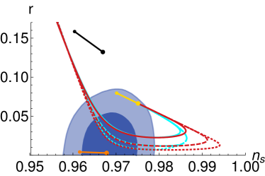
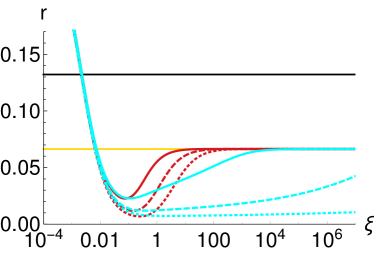
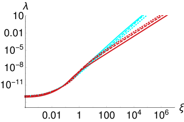
The corresponding results are given in Fig. 1, where we depict vs. (upper panel), vs. (central panel) and vs. (lower panel) for -folds in the metric (cyan) and Palatini formulation (red). Being a relative loop correction we expect it to be smaller666Such a bound comes from the requirement assumed in the beginning of this subsection, , which implies (cf. eqs. (26) and (28)). The region of interest, i.e. the one where we reach the linear attractor, is , which implies . Such an upper bound for is also in agreement with the requirement of a theory always perturbative during all the duration of inflation and with the approximation of eq. (5) with eq. (6). than 1, at least in the region of validity of eq. (6). Therefore we decided to plot our results for the following reference values: (dotted), (dashed) and (continuous). For reference, we also plot the predictions of quadratic (black), linear (yellow) and Starobinsky (orange) inflation in metric gravity. The light blue areas present the 1 and 2 constraints from the BICEP2/Keck data Ade et al. (2016c). Both formulations share the same behaviour. First, for small (), the predictions are aligned with the strong-coupling limit of the standard (without loop corrections) non-minimal inflation Kallosh et al. (2014), then, for large values, the loop correction becomes relevant and the results are departing from the Starobinsky attractor and approaching the linear limit. The bigger , the sooner the predictions departs from the Starobinsky solution. We also notice that in the weak () and strong () coupling limit, which corresponds to the BICEP2/Keck allowed region, the predictions for vs. of the metric and Palatini formulations essentially overlap. The only way to discriminate between the two formulations would be to take into account the reheating phenomenology and the relation between the exact number of -folds and Racioppi (2017). To conclude, we also notice that while the Palatini formulation remains always perturbative () until the linear limit, the metric formulation keeps perturbativity until the linear limit777This improves the previous analysis of Marzola and Racioppi (2016); Artymowski and Racioppi (2017) where perturbativity was not kept until the linear inflation limit because of the use of a too small . only for .
II.2 Induced gravity models
In this subsection we study the phenomenological implications of the non-minimal coupling in eq. (16). In this case we assume that the potential is well described by eqs. (3) and (6) not only in the inflationary region but also around the minimum of the potential. Therefore the loop correction in eq. (6) induces an inflaton VEV
| (26) |
which generates dynamically the Einstein-Hilbert term otherwise missing in eq. (1). We can see that in this scenario the relative loop correction and the non-minimal coupling are correlated via eq. (26). Notice that the requirement allows also for negative . As , the stability of the potential and therefore consistency of the model is ensured by the constraint . We can use the relation (26) to remove the dependence of the potential, obtaining the following Einstein frame scalar potential
| (27) |
where we used eqs. (2) and (26) to express as a function and . As before, the difference between the metric and the Palatini formulations is given by the different expressions for . Taking into account that is not any more a free parameter but (see eq. (26))
| (28) |
it is easy to check that also in this case the field redefinition of eq. (18) and the strong coupling limit () approximation for the potential in eq. (19) still hold. Therefore, also in this case we generate a linear inflation attractor independently of the adopted gravity formulation. For completeness, we perform again a full inflationary analysis considering also values outside the strong coupling limit.
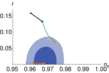
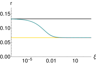
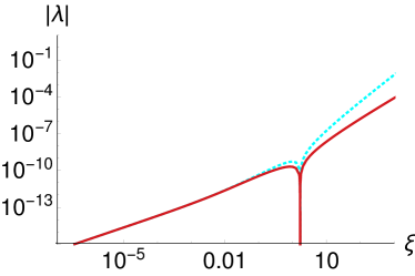
The corresponding results are given in Fig. 2 where we depict vs. (upper panel), vs. (central panel) and the absolute value of () vs. (lower panel) for -folds in the metric (cyan, dashed) and Palatini formulation (red) in the induced gravity scenario. For reference, we also plot the predictions of quadratic (black), linear (yellow) and Starobinsky (orange) inflation in metric gravity. The light blue areas present the 1 and 2 constraints from the BICEP2/Keck data Ade et al. (2016c). As already shown in Racioppi (2017), the predictions are confined in between those of quadratic and linear inflation and it is essentially impossible to distinguish between the two formulations without taking into account reheating. For more details, we refer the reader to Racioppi (2017). In addition to the study of Racioppi (2017), we show here explicitly that the model remains perturbative until the linear limit in both the formulations. The cusp in the vs. plot at is an effect of the logarithmic scale. Such a value corresponds to the case (and therefore ) and it means that our parametrization is not a good one for such a value of . However, it can be shown that the model is perfectly consistent, since the product remains finite.
III Conclusions
We performed an analysis of models of quartic inflation where the inflaton field is subject to relevant loop corrections and it is coupled non-minimally to gravity. We considered two types of quadratic non-minimal couplings: Higgs-inflation-like and induced gravity one. For both of these, we studied the predictions of two different formulations of gravity: metric and Palatini. We showed that in all the cases studied the famous Starobinsky attractor is lost, having been replaced by linear inflation. We stress that the existence of such property is universal i.e. independent of the underlying theory of gravity.
Acknowledgements
The author thanks Martti Raidal, Luca Marzola and Michał Artymowski for useful discussions. This work was supported by the Estonian Research Council grants IUT23-6, PUT1026, and by the ERDF Centre of Excellence project TK133.
References
- Starobinsky (1980) A. A. Starobinsky, Phys. Lett. B91, 99 (1980).
- Guth (1981) A. H. Guth, Phys.Rev. D23, 347 (1981).
- Linde (1982) A. D. Linde, Phys.Lett. B108, 389 (1982).
- Albrecht and Steinhardt (1982) A. Albrecht and P. J. Steinhardt, Phys.Rev.Lett. 48, 1220 (1982).
- Ade et al. (2015) P. A. R. Ade et al. (BICEP2, Planck), Phys. Rev. Lett. 114, 101301 (2015), arXiv:1502.00612 [astro-ph.CO] .
- Ade et al. (2016a) P. A. R. Ade et al. (Planck), Astron. Astrophys. 594, A13 (2016a), arXiv:1502.01589 [astro-ph.CO] .
- Ade et al. (2016b) P. A. R. Ade et al. (Planck), Astron. Astrophys. 594, A20 (2016b), arXiv:1502.02114 [astro-ph.CO] .
- Ade et al. (2016c) P. A. R. Ade et al. (BICEP2, Keck Array), Phys. Rev. Lett. 116, 031302 (2016c), arXiv:1510.09217 [astro-ph.CO] .
- Boubekeur and Lyth (2005) L. Boubekeur and D. H. Lyth, JCAP 0507, 010 (2005), arXiv:hep-ph/0502047 [hep-ph] .
- McAllister et al. (2010) L. McAllister, E. Silverstein, and A. Westphal, Phys. Rev. D82, 046003 (2010), arXiv:0808.0706 [hep-th] .
- Iso et al. (2015) S. Iso, K. Kohri, and K. Shimada, Phys. Rev. D91, 044006 (2015), arXiv:1408.2339 [hep-ph] .
- Kannike et al. (2016) K. Kannike, A. Racioppi, and M. Raidal, JHEP 01, 035 (2016), arXiv:1509.05423 [hep-ph] .
- Rinaldi et al. (2016) M. Rinaldi, L. Vanzo, S. Zerbini, and G. Venturi, Phys. Rev. D93, 024040 (2016), arXiv:1505.03386 [hep-th] .
- Barrie et al. (2016) N. D. Barrie, A. Kobakhidze, and S. Liang, Phys. Lett. B756, 390 (2016), arXiv:1602.04901 [gr-qc] .
- Artymowski and Racioppi (2017) M. Artymowski and A. Racioppi, JCAP 1704, 007 (2017), arXiv:1610.09120 [astro-ph.CO] .
- Racioppi (2017) A. Racioppi, JCAP 1712, 041 (2017), arXiv:1710.04853 [astro-ph.CO] .
- Karam et al. (2017a) A. Karam, L. Marzola, T. Pappas, A. Racioppi, and K. Tamvakis, (2017a), arXiv:1711.09861 [astro-ph.CO] .
- Futamase and Maeda (1989) T. Futamase and K.-i. Maeda, Phys. Rev. D39, 399 (1989).
- Salopek et al. (1989) D. S. Salopek, J. R. Bond, and J. M. Bardeen, Phys. Rev. D40, 1753 (1989).
- Fakir and Unruh (1990) R. Fakir and W. G. Unruh, Phys. Rev. D41, 1783 (1990).
- Amendola et al. (1990) L. Amendola, M. Litterio, and F. Occhionero, Int. J. Mod. Phys. A5, 3861 (1990).
- Kaiser (1995) D. I. Kaiser, Phys. Rev. D52, 4295 (1995), arXiv:astro-ph/9408044 [astro-ph] .
- Bezrukov and Shaposhnikov (2008) F. L. Bezrukov and M. Shaposhnikov, Phys. Lett. B659, 703 (2008), arXiv:0710.3755 [hep-th] .
- Bauer and Demir (2008) F. Bauer and D. A. Demir, Phys. Lett. B665, 222 (2008), arXiv:0803.2664 [hep-ph] .
- Park and Yamaguchi (2008) S. C. Park and S. Yamaguchi, JCAP 0808, 009 (2008), arXiv:0801.1722 [hep-ph] .
- Linde et al. (2011) A. Linde, M. Noorbala, and A. Westphal, JCAP 1103, 013 (2011), arXiv:1101.2652 [hep-th] .
- Kaiser and Sfakianakis (2014) D. I. Kaiser and E. I. Sfakianakis, Phys. Rev. Lett. 112, 011302 (2014), arXiv:1304.0363 [astro-ph.CO] .
- Kallosh and Linde (2013a) R. Kallosh and A. Linde, JCAP 1310, 033 (2013a), arXiv:1307.7938 [hep-th] .
- Kallosh and Linde (2013b) R. Kallosh and A. Linde, JCAP 1312, 006 (2013b), arXiv:1309.2015 [hep-th] .
- Kallosh et al. (2014) R. Kallosh, A. Linde, and D. Roest, Phys. Rev. Lett. 112, 011303 (2014), arXiv:1310.3950 [hep-th] .
- Rubio and Shaposhnikov (2014) J. Rubio and M. Shaposhnikov, Phys. Rev. D90, 027307 (2014), arXiv:1406.5182 [hep-ph] .
- Csaki et al. (2014) C. Csaki, N. Kaloper, J. Serra, and J. Terning, Phys. Rev. Lett. 113, 161302 (2014), arXiv:1406.5192 [hep-th] .
- Galante et al. (2015) M. Galante, R. Kallosh, A. Linde, and D. Roest, Phys. Rev. Lett. 114, 141302 (2015), arXiv:1412.3797 [hep-th] .
- Chiba and Kohri (2015) T. Chiba and K. Kohri, PTEP 2015, 023E01 (2015), arXiv:1411.7104 [astro-ph.CO] .
- Boubekeur et al. (2015) L. Boubekeur, E. Giusarma, O. Mena, and H. Ramírez, Phys. Rev. D91, 103004 (2015), arXiv:1502.05193 [astro-ph.CO] .
- Pieroni (2016) M. Pieroni, JCAP 1602, 012 (2016), arXiv:1510.03691 [hep-ph] .
- Järv et al. (2017) L. Järv, K. Kannike, L. Marzola, A. Racioppi, M. Raidal, M. Rünkla, M. Saal, and H. Veermäe, Phys. Rev. Lett. 118, 151302 (2017), arXiv:1612.06863 [hep-ph] .
- Salvio (2017) A. Salvio, Eur. Phys. J. C77, 267 (2017), arXiv:1703.08012 [astro-ph.CO] .
- Rasanen and Wahlman (2017) S. Rasanen and P. Wahlman, JCAP 1711, 047 (2017), arXiv:1709.07853 [astro-ph.CO] .
- Tenkanen (2017) T. Tenkanen, JCAP 1712, 001 (2017), arXiv:1710.02758 [astro-ph.CO] .
- Birrell and Davies (1984) N. D. Birrell and P. C. W. Davies, Quantum Fields in Curved Space, Cambridge Monographs on Mathematical Physics (Cambridge Univ. Press, Cambridge, UK, 1984).
- Tamanini and Contaldi (2011) N. Tamanini and C. R. Contaldi, Phys. Rev. D83, 044018 (2011), arXiv:1010.0689 [gr-qc] .
- Bauer and Demir (2011) F. Bauer and D. A. Demir, Phys. Lett. B698, 425 (2011), arXiv:1012.2900 [hep-ph] .
- Markkanen et al. (2017) T. Markkanen, T. Tenkanen, V. Vaskonen, and H. Veermäe, (2017), arXiv:1712.04874 [gr-qc] .
- Järv et al. (2017) L. Järv, A. Racioppi, and T. Tenkanen, (2017), arXiv:1712.08471 [gr-qc] .
- Kannike et al. (2014) K. Kannike, A. Racioppi, and M. Raidal, JHEP 06, 154 (2014), arXiv:1405.3987 [hep-ph] .
- Marzola et al. (2016) L. Marzola, A. Racioppi, M. Raidal, F. R. Urban, and H. Veermäe, JHEP 03, 190 (2016), arXiv:1512.09136 [hep-ph] .
- Marzola and Racioppi (2016) L. Marzola and A. Racioppi, JCAP 1610, 010 (2016), arXiv:1606.06887 [hep-ph] .
- Dimopoulos et al. (2017) K. Dimopoulos, C. Owen, and A. Racioppi, (2017), arXiv:1706.09735 [hep-ph] .
- Kannike et al. (2015) K. Kannike, G. Hütsi, L. Pizza, A. Racioppi, M. Raidal, A. Salvio, and A. Strumia, JHEP 05, 065 (2015), arXiv:1502.01334 [astro-ph.CO] .
- Farzinnia and Kouwn (2016) A. Farzinnia and S. Kouwn, Phys. Rev. D93, 063528 (2016), arXiv:1512.05890 [hep-ph] .
- Kannike et al. (2017) K. Kannike, A. Racioppi, and M. Raidal, Nucl. Phys. B918, 162 (2017), arXiv:1605.09378 [hep-ph] .
- Koivisto and Kurki-Suonio (2006) T. Koivisto and H. Kurki-Suonio, Class. Quant. Grav. 23, 2355 (2006), arXiv:astro-ph/0509422 [astro-ph] .
- Prokopec and Weenink (2013) T. Prokopec and J. Weenink, JCAP 1309, 027 (2013), arXiv:1304.6737 [gr-qc] .
- Järv et al. (2015) L. Järv, P. Kuusk, M. Saal, and O. Vilson, Phys. Rev. D91, 024041 (2015), arXiv:1411.1947 [gr-qc] .
- Kuusk et al. (2016a) P. Kuusk, L. Järv, and O. Vilson, Int. J. Mod. Phys. A31, 1641003 (2016a), arXiv:1509.02903 [gr-qc] .
- Kuusk et al. (2016b) P. Kuusk, M. Rünkla, M. Saal, and O. Vilson, Class. Quant. Grav. 33, 195008 (2016b), arXiv:1605.07033 [gr-qc] .
- Flanagan (2004) E. E. Flanagan, Class. Quant. Grav. 21, 3817 (2004), arXiv:gr-qc/0403063 [gr-qc] .
- Catena et al. (2007) R. Catena, M. Pietroni, and L. Scarabello, Phys. Rev. D76, 084039 (2007), arXiv:astro-ph/0604492 [astro-ph] .
- Barvinsky et al. (2008) A. O. Barvinsky, A. Yu. shchik, and A. A. Starobinsky, JCAP 0811, 021 (2008), arXiv:0809.2104 [hep-ph] .
- De Simone et al. (2009) A. De Simone, M. P. Hertzberg, and F. Wilczek, Phys. Lett. B678, 1 (2009), arXiv:0812.4946 [hep-ph] .
- Barvinsky et al. (2009) A. O. Barvinsky, A. Yu. Kamenshchik, C. Kiefer, A. A. Starobinsky, and C. Steinwachs, JCAP 0912, 003 (2009), arXiv:0904.1698 [hep-ph] .
- Steinwachs and Kamenshchik (2011) C. F. Steinwachs and A. Yu. Kamenshchik, Phys. Rev. D84, 024026 (2011), arXiv:1101.5047 [gr-qc] .
- Chiba and Yamaguchi (2013) T. Chiba and M. Yamaguchi, JCAP 1310, 040 (2013), arXiv:1308.1142 [gr-qc] .
- George et al. (2014) D. P. George, S. Mooij, and M. Postma, JCAP 1402, 024 (2014), arXiv:1310.2157 [hep-th] .
- Postma and Volponi (2014) M. Postma and M. Volponi, Phys. Rev. D90, 103516 (2014), arXiv:1407.6874 [astro-ph.CO] .
- Kamenshchik and Steinwachs (2015) A. Yu. Kamenshchik and C. F. Steinwachs, Phys. Rev. D91, 084033 (2015), arXiv:1408.5769 [gr-qc] .
- George et al. (2016) D. P. George, S. Mooij, and M. Postma, JCAP 1604, 006 (2016), arXiv:1508.04660 [hep-th] .
- Miao and Woodard (2015) S. P. Miao and R. P. Woodard, JCAP 1509, 022 (2015), arXiv:1506.07306 [astro-ph.CO] .
- Inagaki et al. (2015) T. Inagaki, R. Nakanishi, and S. D. Odintsov, Phys. Lett. B745, 105 (2015), arXiv:1502.06301 [hep-ph] .
- Burns et al. (2016) D. Burns, S. Karamitsos, and A. Pilaftsis, Nucl. Phys. B907, 785 (2016), arXiv:1603.03730 [hep-ph] .
- Hamada et al. (2017) Y. Hamada, H. Kawai, Y. Nakanishi, and K.-y. Oda, Phys. Rev. D95, 103524 (2017), arXiv:1610.05885 [hep-th] .
- Fumagalli and Postma (2016) J. Fumagalli and M. Postma, JHEP 05, 049 (2016), arXiv:1602.07234 [hep-ph] .
- Fumagalli (2017) J. Fumagalli, Phys. Lett. B769, 451 (2017), arXiv:1611.04997 [hep-th] .
- Bezrukov et al. (2017) F. Bezrukov, M. Pauly, and J. Rubio, (2017), arXiv:1706.05007 [hep-ph] .
- Karam et al. (2017b) A. Karam, T. Pappas, and K. Tamvakis, Phys. Rev. D96, 064036 (2017b), arXiv:1707.00984 [gr-qc] .
- Narain (2017) G. Narain, JCAP 1710, 032 (2017), arXiv:1708.00830 [gr-qc] .
- Ruf and Steinwachs (2017) M. S. Ruf and C. F. Steinwachs, (2017), arXiv:1711.07486 [gr-qc] .
- Ferreira et al. (2018) P. G. Ferreira, C. T. Hill, and G. G. Ross, (2018), arXiv:1801.07676 [hep-th] .
- Zee (1979) A. Zee, Phys. Rev. Lett. 42, 417 (1979).
- Smolin (1979) L. Smolin, Nuclear Physics B 160, 253 (1979).
- Cooper and Venturi (1981) F. Cooper and G. Venturi, Phys. Rev. D 24, 3338 (1981).
- Spokoiny (1984) B. Spokoiny, Physics Letters B 147, 39 (1984).
- Cervantes-Cota and Dehnen (1995a) J. L. Cervantes-Cota and H. Dehnen, Phys. Rev. D51, 395 (1995a), arXiv:astro-ph/9412032 [astro-ph] .
- Cervantes-Cota and Dehnen (1995b) J. L. Cervantes-Cota and H. Dehnen, Nucl. Phys. B442, 391 (1995b), arXiv:astro-ph/9505069 [astro-ph] .
- Lyth and Riotto (1999) D. H. Lyth and A. Riotto, Phys. Rept. 314, 1 (1999), arXiv:hep-ph/9807278 [hep-ph] .