Modeling tagged pedestrian motion: a mean-field type game approach

Abstract

This paper suggests a model for the motion of tagged pedestrians: pedestrians moving towards a specified targeted destination, which they are forced to reach. It aims to be a decision-making tool for the positioning of fire fighters, security personnel and other services in a pedestrian environment. Taking interaction with the surrounding crowd into account leads to a differential nonzero-sum game model where the tagged pedestrians compete with the surrounding crowd of ordinary pedestrians. When deciding how to act, pedestrians consider crowd distribution-dependent effects, like congestion and crowd aversion. Including such effects in the parameters of the game, makes it a mean-field type game. The equilibrium control is characterized, and special cases are discussed. Behavior in the model is studied by numerical simulations.

MSC 2010: 49N90, 49J55, 60H10, 60K30, 91A80, 93E20

Keywords: pedestrian dynamics; backward-forward stochastic differential equations; mean-field type games; congestion; crowd aversion; evacuation planning

1 Introduction

Tagged pedestrians are individuals that plan their motion from an unspecified initial position in order to reach a specified target location in a certain time. The model for tagged pedestrian motion proposed in this paper is based on mean-field type game theory, and is a decision making tool for the positioning of fire fighters, medical personnel, etc, during mass gatherings. The tagged’s prime objective is the pre-set final destination which is considered essential to reach; ending up in proximity of the final destination is not acceptable, it has to be reached. This is in sharp contrast to the standard finite-horizon models cited below, where pedestrians are penalized if their final position deviates from a target position, such penalization is a ’soft’ constraint and can be broken at a cost. The tagged’s initial position is chosen rationally. Therefore, we are inclined to think of the tagged as external entities to be deployed in the crowd. Where they (rationally) ought to be deployed is subject to an offline calculation made by a coordinator: a central planner. Besides tagged pedestrian motion, possible applications of the model include cancer cell dynamics and smart medicine in the human body, and malware propagation in a network, among other.
The central planner’s decision making is based on knowledge of the pedestrian distribution. As noted in [45], the pedestrian behavior in dense crowds is empirically random to some extent, likely due to the large number of external inputs. In a noisy environment, the central planner anticipates the behavior of the crowd and predicts the tagged’s path to the target. As is standard in the mean-field approach, interaction with tagged and ordinary pedestrians is modeled as reactions to the state distribution of a representative tagged and ordinary pedestrian, respectively. This leads us to formulate a mean-field type game based model, which in certain scenarios reduces to an optimal control based model.

1.1 Related work

1.1.1 Optimal control and games of mean-field type

Rational pedestrian behavior is, in this paper, characterized by either a game equilibrium, or an optimal control. The tool used to find the equilibrium/optimal behavior is Pontryagin’s stochastic maximum principle (SMP). For stochastic control problems, SMP yields, when available, necessary conditions that must be satisfied by any optimal solution. The necessary conditions become sufficient under additional convexity conditions. Early results show that an optimal control along with the corresponding optimal state trajectory must solve the so-called Hamiltonian system, which is a two-point (forward-backward) boundary value problem, together with a maximum condition of the so-called Hamiltonian function (see [51] for a detailed account). In stochastic differential games, both zero-sum and nonzero-sum, SMP is one of the main tools for obtaining conditions for an equilibrium, essentially inherited from the theory of stochastic optimal control. For recent examples of the use of SMP in stochastic differential game theory, see [43, 4].
In stochastic systems, the backward equation is fundamentally different from the forward equation, if the solution is required to be adapted. An adapted solution to a backward stochastic differential equation (BSDE) is a pair of adapted stochastic processes $(Y_{\cdot},Z_{\cdot})$, where $Z_{\cdot}$ corrects any “non-adaptedness” caused by the terminal condition of $Y_{\cdot}$. As pointed out in [38], the first component $Y_{\cdot}$ corresponds to the mean evolution of the dynamics, and $Z_{\cdot}$ to the risk between current time and terminal time. Linear BSDEs extend to non-linear BSDEs [46] and backward-forward SDEs (BFSDE) [3, 31]. BSDEs with distribution-dependent coefficients, mean-field BSDEs, are by now well-understood objects [12, 14]. Mean-field BFSDEs arise naturally in the probabilistic analysis of mean-field games (MFG), mean-field type games (MFTG) and optimal control of mean-field type equations.
The theory of optimal control of mean-field SDEs, initiated in [2], treats stochastic control problems with coefficients dependent on the marginal state-distribution. This theory is by now well developed for forward stochastic dynamics, i.e., with initial conditions on state [10, 26, 13, 19]. With SMPs for optimal control problems of mean-field type at hand, MFTG theory can inherit these techniques, just like stochastic differential game theory does in the mean-field free case. See [47] for a review of solution approaches to MFTGs.
Optimal control of mean-field BSDEs has recently gained attention. In [42] the mean-field LQ BSDE control problem with deterministic coefficients is studied. Assuming the control space is linear, linear perturbation is used to derive a stationarity condition which together with a mean-field FBSDE system characterizes the optimal control. Other recent work on the control of mean-field BSDEs makes use of the SMP approach of [50] to control of BFSDEs.
Optimal control problems of mean-field type can be interpreted as large population limits of cooperative games, where the players collaborate to optimize a joint objective [40]. A close relative to mean-field type control is MFG, a class of non-cooperative stochastic differential games, initiated by [34] and [41] independently. For both mean-field type control problems and MFG, the games approximated are games between a large number of indistinguishable (anonymous) players, interacting weakly through a mean-field coupling term. Weak player-to-player interaction through the mean-field coupling restricts the influence one player has on any other player to be inversely proportional to the number of players, hence the level of influence of any specific player is very small. In contrast to the MFG, players in a MFTG can be influential, and distinguishable (non-anonymous). That is, state dynamics and/or cost need not be of the same form over the whole player population, and a single player can have a major influence on other players’ dynamics and/or cost.

1.1.2 Pedestrian crowd modeling

There is a variety of mathematical approaches to the modeling of pedestrian crowd motion. Microscopic force-based models [29, 20], and in particular the social force model, represent pedestrian behavior as a reaction to forces and potentials, applied not only by the surrounding environment but also by the pedestrian’s internal motivation and desire. A cellular automata approach to microscopic modeling of pedestrian crowds can be found in [17, 37, 36], to mention only few. Macroscopic models view the crowd as a continuum, described by averaged quantities such as density and pressure. The Hughes model [35, 33, 48] couples a conservation law, representing the physics of the crowd, with an Eikonal equation modeling a common task of the pedestrians. Its variations are manifold. Kinetic and other multi-scale models [7, 22, 6] constitute an intermediate step between the micro- and the macro scales. Microscopic game and optimal control models for pedestrian crowd dynamics, with their relevant continuum limits in the form of mean-field games and mean-field type optimal control, have gained interest in the last decade. In [30], a simplified MFG was used to model rational behavior of pedestrian in a crowd. Following Lasry and Lion’s paper on MFG, [27] applied MFG to pedestrian crowd motion and [39] used MFG to model local congestion effects, i.e. the relationship between energy needed to walk/run and local crowd density. MFG based models have also been used to simulate evacuation of pedestrians [15, 16, 25].
The mean-field approach rests on an exchangeability assumption; pedestrians are anonymous, they may have different paths but one individual cannot be distinguished from another. While interesting when modeling circumstances where pedestrians can be considered indistinguishable, for instance a train station during rush hour or fast exits of an area in case of an alarm, there are situations where an anonymous crowd model is not satisfactory. Mean-field type games is a tool to extend the mean-field approach to distinguishable sub-crowds and influential individuals, and was applied in [5]. Other ways to break the anonymity within the mean-field approach are multi-population MFGs [28, 21, 1] and major agent models [32, and references therein].
Another important characteristic of standard MFGs and MFTGs is the assumption of anticipative players. Each player is assumed to predict how the whole population will act in the future, and then pick a strategy accordingly. In a pedestrian crowd setting, this would correspond to pedestrians knowing, most likely by experience, how the surrounding crowd will behave. This is a very high ’level of rationality’, and certainly not appropriate in all scenarios. We refer to [23] for a precise discussion on the level of rationality of pedestrian crowd models, including mean-field games and optimal control of mean-field type based models.

1.2 Paper contribution and outline

This paper investigates a new modeling approach to the motion of pedestrians whose primary objective is to reach a specific target, at a specific time. The model can represent a large group that is steered by a central planner, or a single individual. Even though these pedestrians have certain non-standard goals, they are constrained by the same physical limitations as ordinary pedestrians, and the central planner takes this into consideration. Moreover, the central planner has access to complete information of the surrounding environment, and utilizes it in the decision making process.
The contribution of this paper is a mean-field type game based model for the motion of tagged pedestrians in a surrounding crowd of ’ordinary pedestrians’. The players in the game are crowds, and act under general distribution-dependent dynamics and cost. The tagged pedestrians have a ’hard’ terminal condition, while the ordinary pedestrians have a ’hard’ initial condition, and this results in a state equation in the form of a mean-field BFSDE, representing i) the predicted motion of the tagged towards the target, coupled with ii) the evolution of the surrounding crowd from a known initial configuration.
Rational behavior in the model is characterized with a version of SMP, tailored for the mean-field BFSDE system with mean-field type costs. The central section of this paper is the solved examples, where we illustrate pedestrian behavior in the model. Further directions of research are also outlined.
The tagged pedestrian model is presented in Section 2, which begins in a deterministic setting, to which we gradually add components until the full model is reached. The SMP that gives necessary and sufficient conditions for a pair of equilibrium controls for the mean-field type game is presented in Theorem 2.1. Examples of tagged motion are studied in Section 3. All technical proofs and background theory are moved to the appendix.

2 The tagged pedestrian model

In this section the tagged pedestrian model is introduced. Velocity fields are the driving components in the model and include both small-scale pedestrian interactions and path planning components. The latter is implemented by pedestrians in a rational way: A cost functional summarizing pedestrian preferences is minimized. The former describes involuntary movement over which the pedestrian has no control.

List of symbols

• $T\in(0.\infty)$ – the time horizon.

• $(\Omega,\mathcal{F},\mathbb{F},\mathbb{P})$ – the underlying filtered probability space.

• $\mathcal{P}(\mathbb{R}^{d})$ – the space of probability measures on $(\mathbb{R}^{d},\mathcal{B}(\mathbb{R}^{d}))$.

• $\mathcal{P}_{2}(\mathbb{R}^{d})$ – all square-integrable measures in $\mathcal{P}(\mathbb{R}^{d})$.

• $\mathcal{L}\left(X\right)\in\mathcal{P}(\mathbb{R}^{k})$ – the distribution of the random variable $X\in\mathbb{R}^{k}$ under $\mathbb{P}$.

• $X_{\cdot}$ – the stochastic process $\{X_{t};\,t\geq 0\}$.

• $L^{2}_{\mathcal{F}}(\mathbb{R}^{d})$ – the space of $\mathcal{F}$-measurable square-integrable $\mathbb{R}^{d}$-valued random variables.

2.1 Pedestrian dynamics

In a deterministic setting pedestrian state dynamics are described by ordinary differential equations (ODE). An ordinary pedestrian is initiated at some location $x_{0}\in\mathbb{R}^{d}$, and moves according to an ODE with an initial condition,

$$\begin{cases}\frac{d}{dt}X_{t}=b^{x}_{t},&t\in[0,T],\\ X_{0}=x_{0}.\end{cases}$$ (2.1)

The pedestrian influences its velocity through a control function, $u^{x}_{\cdot}$. The control is assumed to take values in the set $U^{x}\subset\mathbb{R}^{d_{x}}$, $d_{x}\geq 1$. Alongside the control function, $b^{x}_{t}$ may depend on interaction with other pedestrians, for example through collisions. In the literature, the velocity is often split into a behavioral velocity (the control) and an interaction velocity,

$$b^{x}_{t}=u^{x}_{t}+b^{x,\text{int}}_{t}.$$ (2.2)

So on top of any interaction velocity the tagged influences its movement through a control, and this grants it some smartness. As was discussed in the introduction, the pedestrian may foresee crowd movement and act in advance to avoid congested areas and other obstacles. Pedestrian models that considers the behavioral velocity to be an internal choice of the pedestrian leaves the framework of classical particle models and enters decision-based smart models. A summary of the difference between these model classes is found in [45]. Alongside ordinary pedestrians, tagged pedestrians are deployed. They represent a person on a mission, who has to reach a target location $y_{T}\in\mathbb{R}^{d}$ at time $t=T$. In the deterministic setting, the tagged moves according to an ODE with terminal condition,

$$\begin{cases}\frac{d}{dt}Y_{t}=u^{y}_{t}+b^{y,\text{int}}_{t},&t\in[0,T],\ u^{y}_{t}\in U^{y}\subset\mathbb{R}^{d_{y}},\ d_{y}\geq 1,\\ Y_{T}=y_{T}.\end{cases}$$ (2.3)

Just like $u_{\cdot}^{x}$ influences the terminal position of an ordinary pedestrian, so does $u_{\cdot}^{y}$ influence the initial position of a tagged pedestrian. This should be interpreted in the following way: the initial position of the tagged pedestrian is not pre-determined, but depends on the pedestrian’s choice of behavioral velocity. This choice is subject to the terminal condition, and at the same time it adheres to other preferences. For example, if there is a high risk of injury at a certain location $y_{T}$ (doors, stairs, etc.), where is the best spot for a medic to be positioned, so that she can reach $y_{T}$ in time $T$? Certainly not at $y_{T}$, since it is a high risk area. The medic’s initial location is preferably a safe spot, from which it is easy for her to access $y_{T}$, taking surrounding pedestrians and environment into account. This is what should be reflected in the choice of $u_{\cdot}^{y}$.
Pedestrian motion can be considered deterministic if the crowd is sparse, but partially random if the crowd is dense. To capture this, (2.1)-(2.3) is extended to its stochastic counterpart. Let $(\Omega,\mathcal{F},\mathbb{P})$ be a complete probability space, endowed with the filtration $\mathbb{F}=(\mathcal{F}_{t})_{t\geq 0}$, satisfying the usual conditions. Let the space carry $B^{x}_{\cdot}$ and $B^{y}_{\cdot}$, independent $w_{x}$- and $w_{y}$-dimensional $\mathbb{F}$-Wiener processes, and a random variable $y_{T}\in L^{2}_{\mathcal{F}_{T}}(\mathbb{R}^{d})$ independent of $B_{\cdot}:=(B^{x}_{\cdot},B^{y}_{\cdot})^{*}$. The Brownian motion $B_{\cdot}$ is split into $B^{x}_{\cdot}$ and $B^{y}_{\cdot}$ to emphasize modeling features: $B^{x}_{\cdot}$ is the noise that explicitly effects the ordinary pedestrians diffusion, while $B^{y}_{\cdot}$ may be used to model any noise that in addition to $B^{x}_{\cdot}$ effects the tagged. All information in the model up to time $t$ is contained in $\mathcal{F}_{t}$, and a process that depends only on past and current information is called an $\mathcal{F}_{t}$-adapted process. It is natural to require pedestrian motion to be adapted, since pedestrians react causally to the environment. In this random environment, we consider a control to be feasible if it is open-loop adapted and square integrable, i.e. belongs to the sets $\mathcal{U}^{x}$ and $\mathcal{U}^{y}$ for ordinary and tagged pedestrians respectively,

$$\mathcal{U}^{x} :=\left\{u:\Omega\times[0,T]\rightarrow U^{x}\ \big{|}\ u_{\cdot}\text{ is }\mathbb{F}\text{-adapted},\ \mathbb{E}\left[\int_{0}^{T}|u_{s}|^{2}ds\right]<\infty\right\},$$ (2.4)

$$\mathcal{U}^{y} :=\left\{u:\Omega\times[0,T]\rightarrow U^{y}\ \big{|}\ u_{\cdot}\text{ is }\mathbb{F}\text{-adapted},\ \mathbb{E}\left[\int_{0}^{T}|u_{s}|^{2}ds\right]<\infty\right\}.$$

As a demonstration of how randomness effects the tagged model, consider the tagged dynamics with Brownian small-scale interactions and a random terminal condition $y_{T}\in L^{2}_{\mathcal{F}_{T}}(\mathbb{R}^{d})$,

$$\begin{cases}dY_{t}=(u^{y}_{t}+B^{y}_{t})dt,&\forall\ t\in[0,T],\ u^{y}_{\cdot}\in\mathcal{U}^{y},\\ Y_{T}=y_{T}.\end{cases}$$ (2.5)

The naive solution $Y_{t}=y_{T}-\int_{t}^{T}(u^{y}_{s}+B^{y}_{s})ds$ is not $\mathcal{F}_{t}$-adapted, it depends on $(B^{y}_{s};t\leq s\leq T)$! On the other hand,

$$Y_{t}=\mathbb{E}\left[y_{T}-\int_{t}^{T}u^{y}_{s}+B^{y}_{s}ds\ |\ \mathcal{F}_{t}\right]$$ (2.6)

is $\mathcal{F}_{t}$-adapted. If $Y_{t}$ from (2.6) is square-integrable for all $t\in[0,T]$, which it is in the current setup, the Martingale Representation Theorem grants existence of a unique square-integrable $\mathbb{R}^{d\times(w_{x}+w_{y})}$-valued and $\mathcal{F}_{t}$-adapted process $Z_{\cdot}$ such that

$$\begin{cases}Y_{t}-\int_{0}^{t}(u^{y}_{s}+B^{y}_{s})ds=\int_{0}^{t}Z_{s}dB_{s},&\forall t\in[0,T],\\ Y_{T}=y_{T}.\end{cases}$$ (2.7)

Equation (2.7) constitutes a BSDE. The conditional expectation (2.6) can be interpreted as the $L^{2}$-projection of the tagged’s future path onto currently available information. Therefore, a practical interpretation of $Z_{\cdot}$ is that it is a supplementary control used by the tagged, to make its path to $y_{T}$ the ’best prediction’ at any instant in time. From a modeling point of view, the tagged pedestrian thus uses two control processes:

• $u^{y}_{\cdot}$ - to heed preferences on initial position, speed, congestion and more. It is the tagged’s subjective best response to the environment.

• $Z_{\cdot}$ - to predict the best path to $y_{T}$ given $u^{y}_{\cdot}$. It is a square-integrable process, implicitly given by the Martingale Representation Theorem.

Interaction between pedestrians at time $t$ is introduced via the mean-field of ordinary pedestrians, $\mathcal{L}\left(X_{t}\right):=\mathbb{P}\circ(X_{t})^{-1}$, and tagged pedestrians, $\mathcal{L}\left(Y_{t}\right)$. They approximate the over-all behavior of the crowds in the large population limit, under the assumption that within each of the two groups individuals are indistinguishable (anonymous). This assumption is in place throughout the paper. An example of a mean-field dependent preference is the following: to safely accomplish its mission, a security team prefers that no individual deviates too far away from the mean position of the team. Also, effects like congestion, the extra effort needed when moving in a high density area, and aversion, repulsion from other pedestrians, can be captured with distribution dependent coefficients.
In a random environment, with mean-field interactions, we formulate the dynamics of representative group members (ordinary and tagged) in the model as

$$\left\{\begin{aligned} dY_{t}&=b^{y}(t,\Theta^{y}_{t},Z_{t},\Theta^{x}_{t})dt+Z_{t}dB_{t},\\ dX_{t}&=b^{x}(t,\Theta^{y}_{t},Z_{t},\Theta^{x}_{t})dt+\sigma^{x}(t,\theta^{y}_{t},Z_{t},\theta^{x}_{t})dB_{t}^{x},\\ Y_{T}&=y_{T},\qquad X_{0}=x_{0},\end{aligned}\right.$$ (2.8)

where $\Theta^{y}_{t}:=(Y_{t},\mathcal{L}\left(Y_{t}\right),u^{y}_{t})$, $\theta^{y}_{t}:=(Y_{t},\mathcal{L}\left(Y_{t}\right))$ and

$$b^{x},b^{y} :\Omega\times[0,T]\times\mathbb{R}^{d}\times\mathcal{P}(\mathbb{R}^{d})\times U^{y}\times\mathbb{R}^{d\times(w_{x}+w_{y})}\times\mathbb{R}^{d}\times\mathcal{P}(\mathbb{R}^{d})\times U^{x}\rightarrow\mathbb{R},$$ (2.9)

$$\sigma^{x} :\Omega\times[0,T]\times\mathbb{R}^{d}\times\mathcal{P}(\mathbb{R}^{d})\times\mathbb{R}^{d\times(w_{x}+w_{y})}\times\mathbb{R}^{d}\times\mathcal{P}(\mathbb{R}^{d})\rightarrow\mathbb{R}.$$

$\Theta^{x}_{t}$ and $\theta_{t}^{x}$ are defined correspondingly. Distribution-dependence makes (2.8) a so-called controlled mean-field BFSDE. Appendix A summarizes results on existence of unique solutions to mean-field BFSDEs and states assumptions strong enough so that there exists a unique solution to (2.8) given any feasible control pair $(u^{x}_{\cdot},u^{y}_{\cdot})\in\mathcal{U}^{x}\times\mathcal{U}^{y}$. The assumptions are in force throughout this paper.

Remark 2.1.

Fundamental diagrams, that describe the marginal relations between speed, density and flow in a crowd, are not necessary in the construction of $b^{x}$ and $b^{y}$, as functions of crowd density. It is pointed out in [23] that the use of fundamental diagrams in pedestrian crowd models is an artifact from road traffic models, without proper justification in the case of two-dimensional flows. Instead, the more natural (for the purpose of modeling pedestrian crowd motion) multidimensional velocity fields $b^{x}$ and $b^{y}$ are used here.

2.2 Pedestrian preferences

Modeling pedestrian preferences is a delicate task. Not only is gathering of and calibration to empirical data difficult for many reasons, but different setups lead to vastly different mathematical formulations of rationality. The focus in this paper is on setups where pedestrian groups are controlled by a central planner. Other possible setups are discussed in Section 4.
The ordinary and tagged pedestrians pay the cost $f^{x}$ and $f^{y}$ per time unit, respectively,

$$f^{x},f^{y}:\Omega\times[0,T]\times\mathbb{R}^{d}\times\mathcal{P}(\mathbb{R}^{d})\times U^{y}\times\mathbb{R}^{d\times(w_{x}+w_{y})}\times\mathbb{R}^{d}\times\mathcal{P}(\mathbb{R}^{d})\times U^{x}\rightarrow\mathbb{R}.$$ (2.10)

On top of this, ordinary pedestrians pay a terminal cost $h^{x}$ at time $T$, and tagged pedestrians pay an initial cost $h^{y}$ at time $0$,

$$h^{x},h^{y}:\Omega\times\mathbb{R}^{d}\times\mathcal{P}(\mathbb{R}^{d})\times\mathbb{R}^{d}\times\mathcal{P}(\mathbb{R}^{d})\rightarrow\mathbb{R}.$$ (2.11)

Given a control feasible pair $(u^{x}_{\cdot},u^{y}_{\cdot})$ the total cost is $J^{x}:\mathcal{U}^{x}\rightarrow\mathbb{R}$ for the ordinary pedestrian, and $J^{y}:\mathcal{U}^{y}\rightarrow\mathbb{R}$ for the tagged,

$$J^{x}(u^{x}_{\cdot};u^{y}_{\cdot}) :=\mathbb{E}\left[\int_{0}^{T}f^{x}(t,\Theta^{y},Z_{t},\Theta^{x}_{t})dt+h^{x}(\theta^{y}_{T},\theta^{x}_{T})\right],$$ (2.12)

$$J^{y}(u^{y}_{\cdot};u^{x}_{\cdot}) :=\mathbb{E}\left[\int_{0}^{T}f^{y}(t,\Theta^{y},Z_{t},\Theta^{x}_{t})dt+h^{y}(\theta^{y}_{0},\theta^{x}_{0})\right].$$

2.2.1 Mean-field type game

Consider the following situation. Within each crowd, pedestrians cooperate, but on a group-level, the crowds compete. This constitutes a so-called mean-field type game between the crowds. A Nash equilibrium in the game is a pair of feasible controls, $(\hat{u}^{x}_{\cdot},\hat{u}^{y}_{\cdot})\in\mathcal{U}^{x}\times\mathcal{U}^{y}$, satisfying the inequalities

$$\begin{cases}J^{x}(u_{\cdot};\hat{u}^{y}_{\cdot})\geq J^{x}(\hat{u}^{x}_{\cdot};\hat{u}^{y}_{\cdot}),&\forall\,u_{\cdot}\in\mathcal{U}^{x},\\ J^{y}(u_{\cdot};\hat{u}^{x}_{\cdot})\geq J^{y}(\hat{u}^{y}_{\cdot};\hat{u}^{x}_{\cdot}),&\forall\,u_{\cdot}\in\mathcal{U}^{y}.\end{cases}$$ (2.13)

The next result is a Pontryagin’s type stochastic maximum principle, and yields necessary and sufficient conditions for any control pair satisfying (2.13). A proof is provided in Appendix C.

Theorem 2.1.

Suppose that $(\hat{u}^{x}_{\cdot},\hat{u}^{y}_{\cdot})$ is a Nash equilibrium, i.e. satisfies (2.13), and let the regularity assumptions of Lemma C.1 be in force. Denote the corresponding state processes, given by (2.8), by $\hat{X}_{\cdot}$ and $(\hat{Y}_{\cdot},\hat{Z}_{\cdot})$ respectively. Let $(p^{xx}_{\cdot},q^{xx}_{\cdot},q^{xy}_{\cdot})$, $p^{xy}_{\cdot}$, $p^{yy}_{\cdot}$ and $(p^{yx}_{\cdot},q^{yx}_{\cdot},q^{yy}_{\cdot})$ solve the adjoint equations

$$\left\{\begin{aligned} dp^{xx}_{t}&=-\left\{\partial_{x}\hat{H}^{x}_{t}+\mathbb{E}\left[{}^{*}(\partial_{\mu^{x}}\hat{H}^{x}_{t})\right]\right\}dt+q^{xx}_{t}dB^{x}_{t}+q^{xy}_{t}dB^{y}_{t},\\ dp^{xy}_{t}&=-\left\{\partial_{y}\hat{H}^{x}_{t}+\mathbb{E}\left[{}^{*}(\partial_{\mu^{y}}\hat{H}^{x}_{t}\right]\right\}dt-\partial_{z}\hat{H}^{x}_{t}dB_{t},\\ dp^{yy}_{t}&=-\left\{\partial_{y}\hat{H}^{y}_{t}+\mathbb{E}\left[{}^{*}(\partial_{\mu^{y}}\hat{H}^{y}_{t})\right]\right\}dt-\partial_{z}\hat{H}^{y}_{t}dB_{t},\\ dp^{yx}_{t}&=-\left\{\partial_{x}\hat{H}^{y}_{t}+\mathbb{E}\left[{}^{*}(\partial_{\mu^{x}}\hat{H}^{y}_{t})\right]\right\}dt+q^{yx}_{t}dB^{x}_{t}+q^{yy}_{t}dB^{y}_{t},\\ p^{xx}_{T}&=-\left\{\partial_{x}\hat{h}^{x}+\mathbb{E}\left[{}^{*}(\partial_{\mu^{x}}\hat{h}^{x})\right]\right\},\quad p^{xy}_{0}=0,\\ p^{yy}_{0}&=\partial_{y}\hat{h}^{y}+\mathbb{E}\left[{}^{*}(\partial_{\mu^{y}}\hat{h}^{y})\right],\quad p^{yx}_{T}=0,\end{aligned}\right.$$ (2.14)

where $H^{i}$, $i\in\{x,y\}$, is the Hamiltonian, defined by

$$H^{i}(\omega,t,y,\mu^{y},v,z,x,\mu^{x},u,p^{ix},p^{iy},q^{ix}):=\sum_{j\in\{x,y\}}b^{j}(\omega,t,y,\mu^{y},v,z,x,\mu^{x},u)p^{ij}$$ (2.15)

$$+\sigma^{x}(\omega,t,y,\mu^{y},x,\mu^{x})q^{ix}-f^{i}(\omega,t,y,\mu^{y},v,z,x,\mu^{x},u).$$

Then

$$\hat{u}^{x}_{t} =\underset{v\in U^{x}}{\text{argmax}}\ H^{x}(t,\hat{\Theta}^{y}_{t},\hat{Z}_{t},\hat{\theta}^{x}_{t},v,p^{xx}_{t},p^{xy}_{t},q^{xx}_{t}),\quad a.e.\text{-}t,\ \mathbb{P}\text{-}a.s.$$ (2.16)

$$\hat{u}^{y}_{t} =\underset{v\in U^{y}}{\text{argmax}}\ H^{y}(t,\hat{\theta}^{y}_{t},v,\hat{Z}_{t},\hat{\Theta}^{x}_{t},p^{yx}_{t},p^{yy}_{t},q^{yx}_{t}),\quad a.e.\text{-}t,\ \mathbb{P}\text{-}a.s.$$

If furthermore $H^{i}$ is concave in $(y,\mu^{y},v,z,x,\mu^{x},u)$, and $h^{i}$ is convex in $(y,\mu^{y},x,\mu^{x},z)$, $i\in\{x,y\}$, then any feasible control pair satisfying (2.16) is a Nash equilibrium in the mean-field type game.

Remark 2.2.

Note that in the mean-field type game, the tagged can be thought of as a major player, influencing the ordinary crowd. Furthermore, the central planner has access to a model of the ordinary crowd and this is necessary for the determination of the equilibrium control.

2.2.2 Optimal control of mean-field type

If the central planner does not have access to a model of the crowd of ordinary pedestrians, any interaction with the surrounding environment will then enter the tagged model as a random signal. This is covered by the $(\omega,t)$-dependence of $b^{y}$ and $f^{y}$. The mean-field type game then reduces to a so-called optimal control problem of mean-field type,

$$\left\{\begin{aligned} \underset{u^{y}_{\cdot}\in\mathcal{U}^{y}}{\text{min}}&\ \mathbb{E}\left[\int_{0}^{T}f^{y}(t,\Theta^{y}_{t},Z_{t})dt+h^{y}(\theta^{y}_{0},Z_{0})\right],\\ \text{s.t.}&\ \ dY_{t}=b^{y}(t,\Theta^{y}_{t},Z_{t})dt+Z_{t}dB_{t},\\ &\ \ Y_{T}=y_{T}.\end{aligned}\right.$$ (2.17)

Problem (2.17) is a special case of (2.13) and necessary and sufficient conditions follow as a corollary to Theorem 2.1.

Corollary 2.1.

Suppose that $\hat{u}^{y}_{\cdot}$ solves (2.17) and denote the corresponding tagged state $(\hat{Y}_{\cdot},\hat{Z}_{\cdot})$. Let $p_{\cdot}$ solve the adjoint equation

$$\left\{\begin{aligned} dp_{t}&=-\left\{\partial_{y}\mathcal{H}(t,\hat{\Theta}^{y}_{t},\hat{Z}_{t},p_{t})+\mathbb{E}\left[{}^{*}(\partial_{\mu}\mathcal{H}(t,\hat{\Theta}^{y}_{t},\hat{Z}_{t},p_{t})\right]\right\}dt\\ &\quad-\partial_{z}\mathcal{H}(t,\hat{\Theta}^{y}_{t},\hat{Z}_{t},p_{t})dB_{t},\\ p_{0}&=\partial_{y}h^{y}(\hat{\theta}^{y}_{0})+\mathbb{E}\left[{}^{*}(\partial_{\mu}h^{y}(\hat{\theta}^{y}_{0})\right],\end{aligned}\right.$$ (2.18)

where $\mathcal{H}$ is the Hamiltonian

$$\mathcal{H}(\omega,t,y,\mu,v,z,p):=b^{y}(\omega,t,y,\mu,v,z)p-f^{y}(t,y,\mu,v,z).$$ (2.19)

Then

$$\hat{u}^{y}_{t}=\underset{v\in U^{y}}{\text{argmax}}\ \mathcal{H}(t,\hat{\theta}^{y}_{t},v,\hat{Z}_{t},p_{t}),\quad a.e.\text{-}t,\ \mathbb{P}\text{-}a.s.$$ (2.20)

If moreover $\mathcal{H}$ is concave in $(y,\mu,v,z)$ and that $h$ is convex in $(y,\mu)$, then any feasible $\hat{u}^{y}_{\cdot}$ that satisfies (2.20), almost surely for a.e. $t$, is an optimal control to (2.17).

3 Simulations

This section is devoted to numerical simulations of the tagged model under various external influences and internal preferences. First, two scenarios in the optimal control version of the model are considered, including preferences on velocity, avoidance and interaction via the mean position of the group. Secondly, asymmetric bidirectional flow is simulated with the full mean-field type game version of the model. None of the parameters used in the simulations stem from real world measurements, but velocity profiles and the asymmetric bidirectional flow are compared qualitatively with the experimental studies [44] and [52].

3.1 Optimal control: keeping a tagged group together

In this scenario, the common goal of the tagged pedestrians is to stay close to the group mean, while conserving energy and initiating in the proximity of $y_{0}\in\mathbb{R}^{2}$. Distance to the group mean is one of the simplest mean-field effects that can be considered. Nonetheless it is a distribution-dependent quantity, and the control problem characterizing tagged pedestrian behavior in this scenario is the nonstandard optimization problem (3.1). The components of (3.1) are presented in Table 1. There is no surrounding crowd present, only tagged pedestrians occupy the space.

$$\left\{\begin{aligned} \underset{u_{\cdot}\in\mathcal{U}}{\text{min}}&\ \frac{1}{2}\mathbb{E}\left[\int_{0}^{T}\left(\lambda_{\text{cont}}\left(u_{t}^{y}\right)^{2}+\lambda_{\text{attr}}\left(Y_{t}-\mathbb{E}[Y_{t}]\right)^{2}\right)dt+\lambda_{\text{init}}(Y_{0}-y_{0})^{2}\right],\\ \text{s.t.}&\ \ dY_{t}=(u_{t}^{y}+\lambda_{\text{noise}}B_{t})dt+Z_{t}dB_{t},\\ &\ \ Y_{T}=y_{T}.\end{aligned}\right.$$ (3.1)

Velocity component	Form
Internal velocity (control)	$u_{\cdot}^{y}\in\mathcal{U}^{y}$
Acceleration noise	$\lambda_{\text{noise}}B_{\cdot}^{y}$
Preference (penalty)	Form
Energy usage per unit time	$\lambda_{\text{cont}}\left(u_{\cdot}^{y}\right)^{2}$
Distance from group mean per unit time	$\lambda_{\text{attr}}\displaystyle\left(Y_{\cdot}-\mathbb{E}[Y_{\cdot}]\right)^{2}$
Distance from $y_{0}\in\mathbb{R}^{2}$ at $t=0$	$\lambda_{\text{init}}(Y_{0}-y_{0})^{2}$

Table 1: Keeping a tagged group together: components

The scenario is simulated for two sets of parameters, see Table 2. The mean-field BFSDE system of equations characterizing optimal behavior, given by Corollary 2.1, is solved with the least-square Monte Carlo method of [9]. The result is presented in Figure 1. The group walks approximately on the straight line from the starting area to the target point. Remember that the initial position of the tagged is chosen rationally by solving (3.1). There is a trade-off between starting close to $y_{0}$ and walking with high speed, and the groups rationally initiates not at $y_{0}$, but somewhere between $y_{0}$ and $y_{T}$. The group that prefers proximity to other group members does indeed move in a more compact formation. The difference appears clearly when looking at the mean distance-to-mean of the tagged group, see Figure 2.

	$\lambda_{\text{noise}}$	$\lambda_{\text{cont}}$	$\lambda_{\text{attr}}$	$\lambda_{\text{init}}$	$\mathbb{E}[y_{0}]$	$y_{T}$	$T$
Set 1 (with distance-to-mean penalty)	1	50	50	10	[0.1,0.1]	[2,2]	1
Set 2 (without distance-to-mean penalty)	1	50	0	10	[0.1,0.1]	[2,2]	1

Table 2: Keeping a tagged group together: parameter values. The preferred initial position is normally distributed around $[0.1,0.1]$.

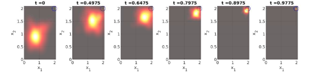
Fig 1: Top row: Crowd density evolution when $\lambda_{2}=50$. Bottom row: Crowd density evolution when $\lambda_{2}=0$.

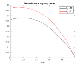
Fig 2: A tagged group acting under preferences with a distance-to-mean penalty indeed moves in a more compact formation than a group that does not.

3.2 Optimal control: desired velocity

Linear-quadratic scenarios have accessible closed form solutions by the method of matching. We want to mention the case where the tagged’s goal is to move at its desired velocity $v_{\text{des}}$, similar to what was originally introduced as the desired speed and direction in [29]. This is an important special case, since desired velocity is measurable in live experiments. See for example [44] for the speed profile of pedestrian walking in a straight corridor, starting from standing still. The scenario is formulated as standard optimal control problem, (3.2), and the setting is summarized in Table 3.

$$\left\{\begin{aligned} \underset{u\in\mathcal{U}[0,T]}{\text{min}}&\ \frac{1}{2}\mathbb{E}\left[\int_{0}^{T}\left(\lambda_{\text{cont}}\left(u_{t}^{y}\right)^{2}+\lambda_{\text{des}}\left(u_{t}^{y}-v_{\text{des}}(t)\right)^{2}+\lambda_{\text{rep}}(Y_{t}-Q)^{2}\right)dt\right],\\ \text{s.t.}&\ \ dY_{t}=(u^{y}_{t}+\lambda_{\text{noise}}B^{y}_{t})dt+Z_{t}dB_{t},\\ &\ \ Y_{T}=y_{T}.\end{aligned}\right.$$ (3.2)

Velocity component	Form
Internal velocity (control)	$u^{y}_{\cdot}\in\mathcal{U}^{y}$
Acceleration noise	$\lambda_{\text{noise}}B_{\cdot}$
Preference	Form
Energy usage per unit time	$\lambda_{\text{cont}}\left(u^{y}_{\cdot}\right)^{2}$
Uncomfortable velocity per unit time	$\lambda_{\text{des}}\left(u^{y}_{\cdot}-v_{\text{des}}(t)\right)^{2}$
Distance from $Q\in\mathbb{R}^{2}$ per unit time	$\lambda_{\text{rep}}(Y_{\cdot}-Q)^{2}$

Table 3: Desired velocity: components

In view of Corollary 2.1, the optimal control is

$$\hat{u}^{y}_{t}=\frac{p_{t}+\lambda_{\text{des}}v_{\text{des}}(t)}{\lambda_{\text{cont}}+\lambda_{\text{rep}}},$$ (3.3)

With the ansatz $\hat{Y}_{t}=\gamma(t)p_{t}+\eta(t)B^{y}_{t}+\theta_{t}$, $\gamma(T)=\eta(T)=0$ and $\theta(T)=y_{T}$, a matching argument gives the optimally controlled dynamics up to a system of ODEs:

$$\begin{cases}\frac{d}{dt}\gamma(t)=-\lambda_{\text{rep}}\gamma(t)^{2}+\frac{1}{\lambda_{\text{cont}}+\lambda_{\text{des}}},&\gamma(T)=0,\\ \frac{d}{dt}\eta(t)=-\lambda_{\text{rep}}\gamma(t)\eta(t)+\lambda_{\text{noise}},&\eta(T)=0,\\ \frac{d}{dt}\theta(t)=-\lambda_{\text{rep}}\gamma(t)(\theta(t)-Q)+\frac{\lambda_{\text{des}}v_{\text{ des}}(t)}{\lambda_{\text{cont}}+\lambda_{\text{des}}},&\theta(T)=y_{T},\\ \hat{Z}_{t}=\eta(t).\end{cases}$$ (3.4)

In Figure 3, the simulated tagged crowd density is presented for two values of $Q$. The desired velocity is set to be negative in both directions for $t\in[0,T/2]$, and positive for $t\in(T/2,T]$, which corresponds to a preference to first move south-west during the first half of the time period and then turn around and move north-east. The parameter $\lambda_{\text{rep}}$ is set to a negative value, hence the tagged prefers to avoid $Q$. Parameters used in the simulation are summarized in Table 4. The trade-off between walking in the desired velocity and walking close to the diamond $Q$ before reaching the target circle is clearly visible. Recall that the initial position is determined by the optimization procedure. In this scenario, there is no preference on initial position and the tagged group compensates for the location of $Q$ by changing its initial position!
In [44] the average time-dependent velocity of a pedestrian initially standing still is measured experimentally in the absence of interactions. The result is a relationship between speed and time, than can be used as data for $v_{\text{des}}$. Approximating the graph presented in [44] with

$$v_{\text{des}}(t)=\max\{0.1,\text{arctan}(\pi t-1.6)\},$$ (3.5)

the scenario is simulated with the two presented in Table 5. The result is presented in Figure 4. The parameter set with a higher penalty on from deviation from desired velocity naturally results in a velocity profile closer to $v_{\text{des}}(t)$.

	$\lambda_{\text{noise}}$	$\lambda_{\text{cont}}$	$\lambda_{\text{des}}$	$\lambda_{\text{rep}}$	$Q$	$v_{\text{des}}(t)$	$y_{T}$	$T$
Set 1	0.5	0.5	1	-2	$[-0.5,-0.5]$	$\text{sign}\left(t-\frac{T}{2}\right)[3,3]$	$[0.1,0.1]$	1
Set 2	0.5	0.5	1	-2	$[1.5,1.5]$	$\text{sign}\left(t-\frac{T}{2}\right)[3,3]$	$[0.1,0.1]$	1

Table 4: Desired velocity: parameter values.

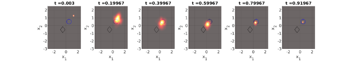
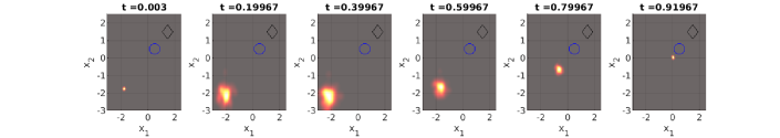
Fig 3: Top row: Desired velocity with Set 1 parameters from Table 4. Bottom row: Desired velocity with Set 2 parameters from Table 4. The tagged crowd moves first south-west and then north-east, following its desired velocity, while avoiding the diamond on its way to the circle.

	$\lambda_{\text{noise}}$	$\lambda_{\text{cont}}$	$\lambda_{\text{des}}$	$\lambda_{\text{rep}}$	$Q$	$v_{\text{des}}(t)$	$y_{T}$	$T$
Set 3	0.1	0.5	2	0	$[0,0]$	Eq. (3.5)	$[0,0]$	4
Set 4	0.1	0.5	10	0	$[0,0]$	Eq. (3.5)	$[0,0]$	4

Table 5: Desired velocity: parameter values.

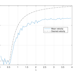
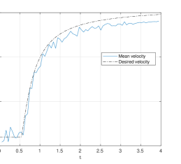
Fig 4: Left: Desired velocity with Set 3 parameters from Table 5. Right: Desired velocity with Set 4 from Table 5. The mean velocity measured in the scenario (3.2) compared to the desired velocity (3.5).

3.3 Mean-field type game: asymmetric bidirectional flow

Consider now a scenario where ordinary pedestrians initiate at $x_{0}\in\mathbb{R}^{2}$, close $y_{T}\in\mathbb{R}^{2}$, the location of an incident. They begin to walk towards the safe spot $x_{T}\in\mathbb{R}^{2}$. A tagged pedestrian is to end up at the location of the incident $y_{T}$ at time $t=T$. The tagged pedestrian is repelled by the mean of the ordinary pedestrian crowd, while the ordinary pedestrian crowd is repelled by the tagged pedestrian. This scenario is implemented as the MFTG (3.6), summarized in Table 6.

$$\begin{cases}J^{x}(u^{x}_{\cdot};u^{y}_{\cdot})=\frac{1}{2}\mathbb{E}\left[\int_{0}^{T}\left(\lambda^{x}_{\text{cont}}\left(u^{x}_{t}\right)^{2}+\lambda^{x}_{\text{rep}}(X_{t}-Y_{t})^{2}\right)dt+\lambda^{x}_{\text{term}}(X_{T}-x_{T})^{2}\right],\\ dX_{t}=u_{t}^{x}dt+\sigma dB^{x}_{t},\quad\sigma\in\mathbb{R},\quad X_{0}=x_{0},\\ J^{y}(u^{y}_{\cdot};u^{x}_{\cdot})=\frac{1}{2}\mathbb{E}\left[\int_{0}^{T}\left(\lambda^{y}_{\text{cont}}\left(u^{y}_{t}\right)^{2}+\lambda^{y}_{\text{red}}(Y_{t}-\mathbb{E}[X_{t}])^{2}\right)dt+\lambda^{y}_{\text{init}}(Y_{0}-y_{0})^{2}\right],\\ dY_{t}=\left(u_{t}^{y}+\lambda^{y}_{\text{noise}}dB^{y}_{t}\right)+Z_{t}dB_{t}.\end{cases}$$ (3.6)

ORDINARY PEDESTRIAN		TAGGED PEDESTRIAN
Velocity component	Form	Velocity component	Form
Internal velocity (control)	$u^{x}_{\cdot}\in\mathcal{U}^{x}$	Internal velocity (control)	$u^{y}_{\cdot}\in\mathcal{U}^{y}$
Diffusion noise level	$\sigma$	Acceleration noise	$\lambda_{\text{noise}}^{y}B^{y}_{\cdot}$
Preference	Form	Preference	Form
Energy usage per unit time	$\lambda^{x}_{\text{cont}}\left(u^{x}_{\cdot}\right)^{2}$	Energy usage per unit time	$\lambda^{y}_{\text{cont}}\left(u^{y}_{\cdot}\right)^{2}$
Repulsion per unit time	$\lambda^{x}_{\text{rep}}(X_{\cdot}-Y_{\cdot})^{2}$	Repulsion per unit time	$\lambda^{y}_{\text{rep}}(Y_{\cdot}-\mathbb{E}[X_{\cdot}])^{2}$
Proximity to $x_{T}$ at $t=T$	$\lambda_{\text{term}}^{x}(X_{T}-x_{T})^{2}$	Proximity to $y_{0}$ at $t=0$	$\lambda_{\text{init}}^{y}(Y_{0}-y_{0})^{2}$

Table 6: Asymmetric bidirectional flow: components

In Figure 5 and Figure 6 the scenario is simulated for the parameter sets presented in Table 7. In Figure 5, the ordinary and the tagged do not have to cross paths to go from their initial to their terminal positions. The simulated paths (top plot of Figure 5) are similar in shape to both the outcome of the corridor experiment under ’condition 3’ (no obstacle) of [44] and the BFR-SSL experiment of [52]. These experimental studies were conducted in a controlled environment that is outside the tagged model presented in this paper. Anyhow, the tagged model replicates the separation of lanes in a bidirectional pedestrian flow and the uncertainty that pedestrian motion exhibits. In the density snapshots (bottom row of Figure 5) reveal that in simulated scenario, the tagged tagged moves in almost constant velocity towards $y_{T}$, while the ordinary group lingers a while at $x_{0}$ before it starts to move towards $x_{T}$. In Figure 6, the tagged’s and the ordinary’s straight path from initiate position to target cross each other. In this scenario, the ordinary pedestrians resolve this by taking walking in a half-circle around the tagged, before moving towards their preferred terminal position $x_{T}$.

TAGGED PEDESTRIAN	$\lambda^{y}_{\text{noise}}$	$\lambda^{y}_{\text{cont}}$	$\lambda^{y}_{\text{rep}}$	$\lambda^{y}_{\text{init}}$	$y_{0}$	$\mathbb{E}[y_{T}]$	$T$
Bidirectional flow	0.7	1	-2	3	[0,1]	[10,0]	1
Twist	0.7	1	-1	3	[0,-3]	[10,-1]	1
ORDINARY PEDESTRIAN	$\sigma$	$\lambda^{x}_{\text{cont}}$	$\lambda^{x}_{\text{rep}}$	$\lambda^{x}_{\text{end}}$	$\mathbb{E}[x_{0}]$	$x_{T}$	$T$
Bidirectional flow	0.7	1	-1	10	[10,-1]	[0,0]	1
Twist	0.7	1	-1.7	10	[10,-2]	[0,0]	1

Table 7: Asymmetric bidirectional flow: parameters values. The initial and terminal constraints are normally distribution with mean tabled above, and standard deviation $0.3$ and $0.1$ for the tagged and ordinary pedestrian, respectively.

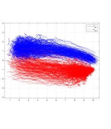
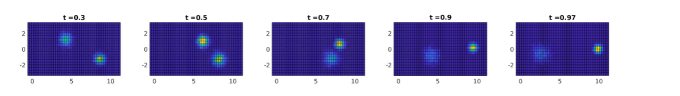
Fig 5: Top row: Pedestrian paths for parameter set ’Bidirectional flow’ from Table 7. Bottom row: Pedestrian density for parameter set ’Bidirectional flow’ from Table 7.

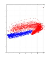
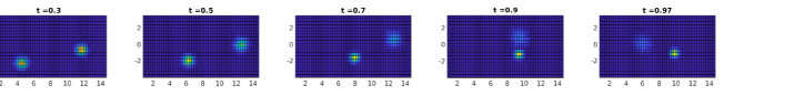
Fig 6: Top row: Pedestrian paths with parameter set ’Twist’ from Table 7. Bottom row: Pedestrian density with parameter set ’Twist’ from Table 7.

4 Concluding remarks and research perspectives

A mean-field type game model for so-called tagged pedestrian motion has been presented and the reliability of the model has been studied through simulations. To perform simulations, necessary and sufficient conditions for a Nash equilibrium are provided in Theorem 2.1. The theorem is proven under quite restrictive conditions on involved coefficient functions. However, necessary conditions for a Nash equilibrium in similar games are available under less restrictive conditions and since our proof follows a standard path, the conditions can certainly be relaxed. The model captures both game-like and minor agent-type scenarios. In the latter, the tagged cannot effect crowd movement while in the former, the tagged and the surrounding crowd have conflicting interests, interact, and compete. The rational pedestrian behavior in the competative game-like scenario is to use an equilibrium strategy.
There are many variations to the mean-field type game approach. The scenarios that have been considered in this paper fall into two rather extreme categories; our pedestrians have acted under either basic or optimal rationality, in the terms of [22]. When pedestrians neither have access to information about their surroundings or the ability to anticipate pedestrian behavior, the best they can do is to implement a control policy based on their own position and target position. This is a basic level of rationality. If the full model is available and pedestrians cooperate, they can implement a control policy of optimal rationality. If the tagged can observe crowd densities at each instant in time but not anticipate future movement, dynamic pedestrian preference may be modeled as a set of control problems: for each $\tau\in[0,T]$,

$$\left\{\begin{aligned} \underset{u^{y}_{.}(\tau)\in\mathcal{U}^{y}_{\tau}}{\text{min}}&\ \mathbb{E}\left[\int_{\tau}^{T}f^{y}(t,Y_{t},\mathcal{L}\left(Y_{\tau}\right),u^{y}_{t}(\tau))dt+\mathbb{I}\{\tau=0\}h^{y}(Y_{0},\mathcal{L}\left(Y_{0}\right))\right],\\ \text{s.t.}&\ \ dY_{t}=b^{y}(t,Y_{t},\mathcal{L}\left(Y_{\tau}\right),Z_{t},u^{y}_{t}(\tau))dt+Z_{t}dB_{t},\\ &\ \ Y_{T}=y_{T},\end{aligned}\right.$$ (4.1)

where $\mathcal{U}^{y}_{\tau}$ is defined in the same way as $\mathcal{U}^{y}$, but with the interval $[0,T]$ replaced by $[\tau,T]$, cf. (2.4). This is an intermediate level between basic and optimal rationality. Pedestrian decision making can also be modeled as a decentralized mechanism, i.e. instead of cooperating, pedestrians compete in a game-like manner within the crowd. Decentralized crowd formation can be modeled by a MFG:

• Fix a deterministic function $\mu_{\cdot}:[0,T]\rightarrow\mathcal{P}_{2}(\mathbb{R}^{d})$.

• Solve the stochastic control problem

  $$\left\{\begin{aligned} \underset{u^{y}_{\cdot}\in\mathcal{U}^{y}}{\text{min}}&\ \mathbb{E}\left[\int_{0}^{T}fy(t,Y_{t},\mu_{t},u^{y}_{t})dt+h^{y}(Y_{0},\mu_{0})\right],\\ \text{s.t.}&\ \ dY_{t}=b(t,Y_{t},\mu_{t},Z_{t},u^{y}_{t})dt+Z_{t}dB_{t},\\ &\ \ Y_{T}=y_{T}.\end{aligned}\right.$$ (4.2)

• Determine the function $\hat{\mu}_{\cdot}:[0,T]\rightarrow\mathcal{P}_{2}(\mathbb{R}^{d})$ such that $\hat{\mu}_{t}$ is the law of the optimally controlled state from Step (ii) at time $t$.

Furthermore, minimal exit time (evacuation) problems can be posed at all levels of rationality.
The numerical simulation of mean-field BFSDE systems is in this paper done either with the least-square Monte Carlo method of [8], or by reducing them to a system of ODEs by the method of matching. The downside with the least-square Monte Carlo method is that it is not clear which basis functions to use and the matching method is feasible only for linear quadratic problems. Other simulation approaches include deep learning [49] and fixed-point schemes [24]. Fast and stable numerical solvers for mean-field BFSDEs beyond the linear-quadratic case is an area of research that would benefit many applied fields. In pedestrian crowd modeling, improved solvers would facilitate simulation when effects like congestion, crowd aversion, and anisotropic preferences are present.

A Mean-field BFSDE

Given a control pair $(u^{x}_{\cdot},u^{y}_{\cdot})\in\mathcal{U}^{x}\times\mathcal{U}^{y}$, systems of the form (2.8) have been studied in the context of optimal control of mean-field type, where they naturally arise as necessary optimality conditions. This appendix summarizes some of the results on existence and uniqueness of solutions to MF-BFSDEs. Let

$$\mathbb{H}^{2,d}:=\left\{V_{\cdot}\ \mathbb{R}^{d}\text{-valued and prog. meas.}\ :\ \mathbb{E}\left[\int_{0}^{T}|V_{s}|^{2}ds\right]<\infty\right\}$$ (A.1)

$$\mathbb{S}^{2,d}:=\left\{V_{\cdot}\ \mathbb{R}^{d}\text{-valued and prog.meas.}\ :\ \mathbb{E}\left[\sup_{s\in[0,T]}|V_{s}|^{2}\right]<\infty\right\}$$

and recall that, in the case of a fixed control pair, $b^{x}$ and $b^{y}$ are functions of

$$(\omega,t,y,\mu^{y},z,x,\mu^{x})\in\Omega\times[0,T]\times\mathbb{R}^{d}\times\mathcal{P}_{2}(\mathbb{R}^{d})\times\mathbb{R}^{d\times(w_{x}+w_{y})}\times\mathbb{R}^{d}\times\mathcal{P}(\mathbb{R}^{d})$$ (A.2)

and $\sigma^{x}$ is a function of

$$(\omega,y,\mu^{y},z,x,\mu^{x})\in\Omega\times\mathbb{R}^{d}\times\mathcal{P}_{2}(\mathbb{R}^{d})\times\mathbb{R}^{d\times(w_{x}+w_{y})}\times\mathbb{R}^{d}\times\mathcal{P}(\mathbb{R}^{d}).$$ (A.3)

A.1 Quadratic-type constraints

For $t\in[0,T]$, $\mu^{y},\mu^{x}\in\mathcal{P}2(\mathbb{R}^{d})$, $x,\bar{x},y,\bar{y}\in\mathbb{R}^{d}$ and $z,\bar{z}\in\mathbb{R}^{d\times(w_{x}+w_{y})}$, let

$$\mathcal{A}(t,y,\bar{y},\mu^{y},v,z,\bar{z},x,\bar{x},\mu^{x})$$ (A.4)

$$=(b^{y}(t,y,\mu^{y},v,z,x,\mu^{x})-b^{y}(t,\bar{y},\mu^{y},v,\bar{z},\bar{x},\mu^{x}))\cdot(y-\bar{y})$$

$$\quad+(b^{x}(t,y,\mu^{y},v,z,x,\mu^{x})-b^{x}(t,\bar{y},\mu^{y},v,\bar{z},\bar{x},\mu^{x}))\cdot(x-\bar{x})$$

$$\quad+(\sigma^{x}(t,y,\mu^{y},z,x,\mu^{x})-\sigma^{x}(t,\bar{y},\mu^{y},\bar{z},\bar{x},\mu^{x}))\cdot(z-\bar{z}).$$

In [24], the authors provide conditions on $\mathcal{A}$ under which, alongside standard assumptions, (2.8) has a unique solution $(X_{\cdot},Y_{\cdot},Z_{\cdot})$ in $\mathbb{H}^{2,d}\times\mathbb{H}^{2,d}\times\mathbb{H}^{2,d\times(w_{x}+w_{y})}$ for all $T$.

A.2 Small time constraint

Under standard Lipschitz- and linear growth-conditions and for a non-degenerate diffusion $\sigma^{x}$, (2.8) has a unique solution $(X_{\cdot},Y_{\cdot},Z_{\cdot})\in\mathbb{S}^{2,d}\times\mathbb{S}^{2,d}\times\mathbb{H}^{2,d\times(w_{x}+w_{y})}$ for small enough $T$ [19]. The bound on $T$ depends on the Lipschitz coefficients. In [19], the authors provide an example where uniqueness fails.

B Differentiation of measure-valued functions

The differentiation of measure-valued functions is handled with the lifting technique, introduced by P.-L. Lions and outlined in for example [18, 11, 19]. Assume that the underlying probability space is rich enough, so that for every $\mu\in\mathcal{P}_{2}(\mathbb{R}^{d})$ there is a random variable $Y\in L^{2}_{\mathcal{F}}(\Omega;\mathbb{R}^{d})$ such that $\mathcal{L}\left(Y\right)=\mu$. A probability space with this property is $([0,1],\mathcal{B}([0,1]),dx)$. Under this assumption, any function $f:\mathcal{P}_{2}(\mathbb{R}^{d})\rightarrow\mathbb{R}$ induces a function $F:L^{2}(\mathbb{R}^{d})\rightarrow\mathbb{R}$ so that $F(Y):=f(\mathcal{L}\left(Y\right))$. The Fréchet derivative of $F$ at $Y$, whenever it exists, is the continuous linear functional $DF[Y]$ that satisfies

$$F(Y^{\prime})-F(Y)=\mathbb{E}\left[DF[Y]\cdot(Y^{\prime}-Y)\right]+o(\|Y^{\prime}-Y\|_{2}),\quad\forall Y^{\prime}\in L^{2}_{\mathcal{F}}(\Omega;\mathbb{R}^{d}).$$ (B.1)

Riesz’ Representation Theorem yields uniqueness of $DF[Y]$. Furthermore, there exists a Borel function $\varphi[\mu]:\mathbb{R}^{d}\rightarrow\mathbb{R}^{d}$, independent of the version of $Y$, such that $DF[Y]=\varphi[\mathcal{L}\left(Y\right)](Y)$ [18]. Therefore

$$f(\mathcal{L}\left(Y^{\prime}\right))-f(\mathcal{L}\left(Y\right))=\mathbb{E}\left[\varphi[Y](Y)(Y^{\prime}-Y)\right]+o(\|Y^{\prime}-Y\|),\quad\forall Y^{\prime}\in L^{2}_{\mathcal{F}}(\Omega;\mathbb{R}^{d}).$$ (B.2)

Denote $\partial_{\mu}f(\mu;x):=\varphi[\mu](x)$, $x\in\mathbb{R}^{d}$, and $\partial_{\mu}f(\mathcal{L}\left((\right)Y);Y)=:\partial_{\mu}f(\mathcal{L}\left((\right)Y))$. The following identity characterizes derivatives with respect to elements in $\mathcal{P}_{2}(\mathbb{R}^{d})$,

$$DF[Y]=\varphi[\mathcal{L}\left(Y\right)](Y)=\partial_{\mu}f(\mathcal{L}\left(Y\right)).$$ (B.3)

Equation (B.2) is the Taylor approximation of a measure-valued function. Consider now an $f$ that besides the measure takes another argument, $\xi$. Then

$$f(\xi,\mathcal{L}\left(Y^{\prime}\right))-f(\xi,\mathcal{L}\left(Y\right))=\mathbb{E}\left[\partial_{\mu}f(\widetilde{\xi},\mathcal{L}\left(Y\right);Y)(Y^{\prime}-Y)\right]+o(\|Y-Y^{\prime}\|_{2}),$$ (B.4)

where the expectation is taken over non-tilded random variables. This is abbreviated as

$$\mathbb{E}\left[\partial_{\mu}f(\widetilde{\xi},\mathcal{L}\left(Y\right);Y)(Y^{\prime}-Y)\right]=:\mathbb{E}\left[(\partial_{\mu}f(\xi,\mathcal{L}\left(Y\right)))^{*}(Y^{\prime}-Y)\right].$$ (B.5)

Note that $\mathcal{L}\left(Y\right)$ is deterministic, so the expectation is only taken over the ’directional argument’ of $\partial_{\mu}f$, $Y$. Also, the expected value (B.5) is stochastic, since it is not taken over $\xi$. Taking another expectation and changing the order of integration yields

$$\mathbb{E}\left[\widetilde{\mathbb{E}}\left[\partial_{\mu}f(\widetilde{\xi},\mathcal{L}\left(Y\right);Y)\right](Y^{\prime}-Y)\right],$$ (B.6)

where the tilded expectation is taken over tilded random variables. This is abbreviated as

$$\widetilde{E}\left[\partial_{\mu}f(\widetilde{\xi},\mathcal{L}\left(Y\right);Y)\right]=:\mathbb{E}\left[{}^{*}(\partial_{\mu}f(\xi,\mathcal{L}\left(Y\right)))\right]$$ (B.7)

Example from Section 3.1 The following measure derivative appears in Section 3.1,

$$\mathbb{E}\left[{}^{*}\left(\partial_{\mu}\left(Y_{t}-\int_{\mathbb{R}^{2}}y\mathcal{L}\left(Y_{t}\right)(dy)\right)^{2}\right)\right].$$ (B.8)

Note that $\left(Y_{t}-\int_{\mathbb{R}^{2}}y\mathcal{L}\left(Y_{t}\right)(dy)\right)^{2}=(Y_{t}-\mathbb{E}\left[M\right])^{2}=:F(M)$ where $M$ is a random variable with probability law $\mathcal{L}\left(Y_{t}\right)$. By the Taylor expansion, $DF[M]=2(Y_{t}-\mathbb{E}\left[M\right])$ and therefore

$$\mathbb{E}\left[{}^{*}\left(\partial_{\mu}\left(Y_{t}-\int_{\mathbb{R}^{2}}y\mathcal{L}\left(Y_{t}\right)(dy)\right)^{2}\right)\right]=\mathbb{E}\left[2(Y_{t}-\mathbb{E}\left[M\right])\right]=0.$$ (B.9)

C Proof of Theorem 2.1

Let $\bar{u}^{x,\epsilon}_{\cdot}$ be a spike variation of $\hat{u}^{x}_{\cdot}$,

$$\bar{u}^{x,\epsilon}_{t}:=\left\{\begin{array}[]{l l}\hat{u}^{x}_{t},&t\in[0,T]\backslash E_{\epsilon},\\ u_{t},&t\in E_{\epsilon},\end{array}\right.$$ (C.1)

where $u_{\cdot}\in\mathcal{U}^{x}$ and $E_{\epsilon}$ is a subset of $[0,T]$ of measure $\epsilon$. Given the control pair $(\bar{u}^{x,\epsilon}_{\cdot},\hat{u}^{y}_{\cdot})$, denote the corresponding solution to the state equation (2.8) by $\bar{X}^{\epsilon}_{\cdot}$ and $(\bar{Y}^{\epsilon}_{\cdot},\bar{Z}^{\epsilon}_{\cdot})$. To ease notation, let for $\vartheta\in\{b^{x},b^{y},\sigma^{x},f^{x},f^{y},h^{x},h^{y}\}$,

$$\bar{\vartheta}^{\epsilon}_{t}:=\vartheta(t,\bar{\theta}^{y,\epsilon}_{t},\hat{u}^{y}_{t},\bar{Z}^{\epsilon}_{t},\bar{\Theta}^{x,\epsilon}_{t}),\ \ \hat{\vartheta}^{\epsilon}_{t}:=\vartheta(t,\hat{\Theta}^{y}_{t},\hat{Z}_{t},\hat{\Theta}^{x}_{t}),\ \ \delta_{x}\vartheta(t):=\vartheta(t,\hat{\Theta}^{y}_{t},\hat{Z}_{t},\hat{\theta}^{x}_{t},\bar{u}^{x,\epsilon}_{t})-\hat{\vartheta}^{\epsilon}_{t}.$$ (C.2)

Consider the ordinary pedestrian’s potential loss, would she switch from the equilibrium control $\hat{u}^{x}_{\cdot}$ to the perturbed $\bar{u}^{x,\epsilon}_{\cdot}$,

$$J^{x}(\bar{u}^{x,\epsilon}_{\cdot};\hat{u}^{y}_{\cdot})-J(\hat{u}^{x}_{\cdot};\hat{u}^{y}_{\cdot}) =\mathbb{E}\left[\int_{0}^{T}\left(\bar{f}^{x,\epsilon}_{t}-\hat{f}^{x}_{t}\right)dt+\bar{h}^{x,\epsilon}_{T}-\hat{h}^{x}_{T}\right].$$ (C.3)

A Taylor expansion of the terminal cost difference yields

$$\mathbb{E}\left[\bar{h}^{x,\epsilon}_{T}-\hat{h}^{x}_{T}\right]=\mathbb{E}\left[\left(\partial_{y}\hat{h}^{x}_{t}+\mathbb{E}[^{*}(\partial_{\mu}\hat{h}^{x}_{T})]\right)\left(\bar{X}^{\epsilon}_{t}-\hat{X}_{t}\right)\right]+o\left(\|\bar{X}^{\epsilon}_{T}-\hat{X}_{T}\|_{2}\right),$$ (C.4)

Let $\widetilde{X}^{x}_{\cdot}$ and $(\widetilde{Y}^{x}_{\cdot},\widetilde{Z}^{x}_{\cdot})$ be the first order variation processes, solving the linear BFSDE system

$$\left\{\begin{aligned} d\widetilde{X}^{x}_{t}&=\Big{\{}\left(\partial_{y}\hat{b}^{x}_{t}+\mathbb{E}[^{*}(\partial_{\mu^{y}}\hat{b}^{x}_{t})]\right)\widetilde{Y}^{x}_{t}+\partial_{z}\hat{b}^{x}_{t}\widetilde{Z}^{x}_{t}+\left(\partial_{x}\hat{b}^{x}_{t}+\mathbb{E}[^{*}(\partial_{\mu^{x}}\hat{b}^{x}_{t})]\right)\widetilde{X}^{x}_{t}\\ \ &\hskip 28.45274pt+\delta_{x}b^{x}(t)1_{E_{\epsilon}}(t)\Big{\}}dt\\ &\quad+\Big{\{}\left(\partial_{y}\hat{\sigma}^{x}_{t}+\mathbb{E}[^{*}(\partial_{\mu^{y}}\hat{\sigma}^{x}_{t})]\right)\widetilde{Y}^{x}_{t}+\partial_{z}\hat{\sigma}^{x}_{t}\widetilde{Z}^{x}_{t}+\left(\partial_{x}\hat{\sigma}^{x}_{t}+\mathbb{E}[^{*}(\partial_{\mu^{x}}\hat{\sigma}^{x}_{t})]\right)\widetilde{X}^{x}_{t}\Big{\}}dB^{x}_{t},\\ d\widetilde{Y}^{x}_{t}&=\Big{\{}\left(\partial_{y}\hat{b}^{y}_{t}+\mathbb{E}[^{*}(\partial_{\mu^{y}}\hat{b}^{y}_{t})]\right)\widetilde{Y}^{x}_{t}+\partial_{z}\hat{b}^{y}_{t}\widetilde{Z}^{x}_{t}+\left(\partial_{x}\hat{b}^{y}_{t}+\mathbb{E}[^{*}(\partial_{\mu^{x}}\hat{b}^{y}_{t})]\right)\widetilde{X}^{x}_{t}\\ \ &\hskip 28.45274pt+\delta_{x}b^{y}(t)1_{E_{\epsilon}}(t)\Big{\}}dt+\widetilde{Z}^{x}_{t}dB_{t},\\ \widetilde{X}^{x}_{0}&=0,\quad\widetilde{Y}^{x}_{T}=0.\end{aligned}\right.$$ (C.5)

Lemma C.1.

Assume that $b^{x}$ are $b^{y}$ are Lipschitz in the controls, that $b^{x},b^{y},f^{x},f^{y}$ and $\sigma^{x}$ are differentiable at the equilibrium point almost surely for all $t$, that their derivatives are bounded almost surely for all $t$ and that

$$\partial_{x}\hat{h}^{x}+\mathbb{E}\left[{}^{*}(\partial_{\mu^{x}}\hat{h}^{x})\right]\in L^{2}_{\mathcal{F}_{T}}(\mathbb{R}^{d}),\quad\partial_{y}\hat{h}^{y}+\mathbb{E}\left[{}^{*}(\partial_{\mu^{y}}\hat{h}^{y})\right]\in L^{2}_{\mathcal{F}_{0}}(\mathbb{R}^{d}).$$ (C.6)

Then for some positive constant $C$,

$$\sup_{t\in[0,T]}\mathbb{E}\left[|\widetilde{X}^{x}_{t}|^{2}+|\widetilde{Y}^{x}_{t}|^{2}+\int_{0}^{t}\|\widetilde{Z}^{x}_{s}\|_{F}\;ds\right]\leq C\epsilon^{2}.$$ (C.7)

$$\sup_{t\in[0,T]}\mathbb{E}\left[|\bar{X}^{\epsilon}_{t}-\hat{X}_{t}-\widetilde{X}^{x}_{t}|^{2}+|\bar{Y}^{\epsilon}_{t}-\hat{Y}_{t}-\widetilde{Y}^{x}_{t}|^{2}+\int_{0}^{t}\|\bar{Z}^{\epsilon}_{s}-\hat{Z}_{s}-\widetilde{Z}^{x}_{s}\|_{F}\;ds\right]\leq C\epsilon^{2}.$$

Proof.

The proof is a combination of standard estimates, see [51] for the SDE terms and [4] for the BSDE terms. ∎

The adjoint processes and the Hamiltonian, defined in (2.14) and (2.15) respectively, yield together with Lemma C.1 and integration by parts that

$$J^{x}(\bar{u}^{x,\epsilon}_{\cdot};\hat{u}^{y}_{\cdot})-J(\hat{u}^{x}_{\cdot};\hat{u}^{y}_{\cdot})=\mathbb{E}\Bigg{[}\int_{0}^{T}\Bigg{\{}\left(\bar{b}^{x,\epsilon}_{t}-\hat{b}^{x}_{t}\right)p^{xx}_{t}+\left(\bar{b}^{y,\epsilon}_{t}-\hat{b}^{y}_{t}\right)p^{xy}_{t}$$ (C.8)

$$\hskip 56.9055pt+\left(\bar{\sigma}^{x,\epsilon}_{t}-\hat{\sigma}^{x}_{t}\right)q^{xx}_{t}-\left(\bar{H}^{x,\epsilon}_{t}-\hat{H}^{x}_{t}\right)\Bigg{\}}dt-p^{xx}_{T}\widetilde{X}^{x}_{T}\Bigg{]}+o(\epsilon)$$

$$=\mathbb{E}\Bigg{[}\int_{0}^{T}\Bigg{\{}\left(\bar{b}^{x,\epsilon}_{t}-\hat{b}^{x}_{t}\right)p^{xx}_{t}+\left(\bar{b}^{y,\epsilon}_{t}-\hat{b}^{y}_{t}\right)p^{xy}_{t}+\left(\bar{\sigma}^{x,\epsilon}_{t}-\hat{\sigma}^{x}_{t}\right)q^{xx}_{t}-\left(\bar{H}^{x,\epsilon}_{t}-\hat{H}^{x}_{t}\right)\Bigg{\}}dt$$

$$\hskip 56.9055pt-\int_{0}^{T}\widetilde{X}^{x}_{t}dp^{xx}_{t}-\int_{0}^{T}p^{xx}_{t}d\widetilde{X}^{x}_{t}-\int_{0}^{T}d\langle p^{xx}_{\cdot},\widetilde{X}^{x}_{\cdot}\rangle_{t}$$

$$\hskip 56.9055pt-\int_{0}^{T}\widetilde{Y}^{x}_{t}dp^{xy}_{t}-\int_{0}^{T}p^{xy}_{t}d\widetilde{Y}^{x}_{t}-\int_{0}^{T}d\langle p^{xy}_{\cdot},\widetilde{Y}^{x}_{\cdot}\rangle_{t}\Bigg{]}+o(\epsilon)$$

$$=-\mathbb{E}\left[\int_{0}^{T}\delta_{x}H^{x}(t)1_{E_{\epsilon}}(t)dt\right]+o(\epsilon),$$

where $\bar{H}^{x,\epsilon}_{t},\hat{H}^{x}_{t}$ and $\delta_{x}H^{x}(t)$ are defined in line with (C.2). The final equality is retrieved by expanding all differences on the third row of (C.8), canceling all but $\delta_{x}H^{x}(t)1_{E_{\epsilon}}(t)$ with the forth and fifth row, while making use of the estimates from Lemma C.1.
Consider now a spike variation of the tagged’s control,

$$\check{u}^{y,\epsilon}_{t}:=\left\{\begin{array}[]{l l}\hat{u}^{y}_{t},&t\in[0,T]\backslash E_{\epsilon},\\ u_{t},&t\in E_{\epsilon},\end{array}\right.$$ (C.9)

where $u_{\cdot}\in\mathcal{U}^{y}$. Following the same lines of calculations as above, one finds that if $p^{yx}_{\cdot}$, $p^{yy}_{\cdot}$ are given by the adjoint equations (2.14) and the Hamiltonian $H^{y}$ by (2.15), then

$$J^{y}(\check{u}^{y,\epsilon}_{\cdot};\hat{u}^{x}_{\cdot})-J^{y}(\hat{u}^{y}_{\cdot};\hat{u}^{x}_{\cdot})=-\mathbb{E}\left[\int_{0}^{T}\delta_{y}H^{y}(t)1_{E_{\epsilon}}dt\right]+o(\epsilon),$$ (C.10)

where $\delta_{y}H^{y}(t)$ is defined in line with (C.2), for the spike perturbation $\check{u}^{y,\epsilon}_{t}$. The rest of the proof is standard, and can be found in for example [51].

References

- [1] Yves Achdou, Martino Bardi, and Marco Cirant. Mean field games models of segregation. Mathematical Models and Methods in Applied Sciences, 27(01):75–113, 2017.
- [2] Daniel Andersson and Boualem Djehiche. A maximum principle for SDEs of mean-field type. Applied Mathematics & Optimization, 63(3):341–356, 2011.
- [3] Fabio Antonelli. Backward-forward stochastic differential equations. The Annals of Applied Probability, pages 777–793, 1993.
- [4] Alexander Aurell. Mean-field type games between two players driven by backward stochastic differential equations. Games, 9(4):88, 2018.
- [5] Alexander Aurell and Boualem Djehiche. Mean-field type modeling of nonlocal crowd aversion in pedestrian crowd dynamics. SIAM Journal on Control and Optimization, 56(1):434–455, 2018.
- [6] N Bellomo, D Clarke, L Gibelli, P Townsend, and BJ Vreugdenhil. Human behaviours in evacuation crowd dynamics: from modelling to “big data” toward crisis management. Physics of life reviews, 18:1–21, 2016.
- [7] Nicola Bellomo, Abdelghani Bellouquid, and Damian Knopoff. From the microscale to collective crowd dynamics. Multiscale Modeling & Simulation, 11(3):943–963, 2013.
- [8] Christian Bender and Jessica Steiner. A posteriori estimates for backward SDEs. SIAM/ASA Journal on Uncertainty Quantification, 1(1):139–163, 2013.
- [9] Christian Bender, Jianfeng Zhang, et al. Time discretization and markovian iteration for coupled FBSDEs. The Annals of Applied Probability, 18(1):143–177, 2008.
- [10] Alain Bensoussan, Jens Frehse, Phillip Yam, et al. Mean field games and mean field type control theory, volume 101. Springer, 2013.
- [11] Rainer Buckdahn, Boualem Djehiche, and Juan Li. A general stochastic maximum principle for SDEs of mean-field type. Applied Mathematics & Optimization, 64(2):197–216, 2011.
- [12] Rainer Buckdahn, Boualem Djehiche, Juan Li, Shige Peng, et al. Mean-field backward stochastic differential equations: a limit approach. The Annals of Probability, 37(4):1524–1565, 2009.
- [13] Rainer Buckdahn, Juan Li, and Jin Ma. A stochastic maximum principle for general mean-field systems. Applied Mathematics & Optimization, 74(3):507–534, 2016.
- [14] Rainer Buckdahn, Juan Li, and Shige Peng. Mean-field backward stochastic differential equations and related partial differential equations. Stochastic Processes and their Applications, 119(10):3133–3154, 2009.
- [15] Martin Burger, Marco Di Francesco, Peter A Markowich, and Marie Therese Wolfram. Mean field games with nonlinear mobilities in pedestrian dynamics. Discrete and Continuous Dynamical Systems-Series B, 2014.
- [16] Martin Burger, Marco Di Francesco, Peter A Markowich, and Marie-Therese Wolfram. Mean field games with nonlinear mobilities in pedestrian dynamics. Discrete and Continuous Dynamical Systems-Series B, 19(5):1311–1333, 2014.
- [17] Carsten Burstedde, Kai Klauck, Andreas Schadschneider, and Johannes Zittartz. Simulation of pedestrian dynamics using a two-dimensional cellular automaton. Physica A: Statistical Mechanics and its Applications, 295(3):507–525, 2001.
- [18] Pierre Cardaliaguet. Notes on mean field games. Technical report, 2010.
- [19] René Carmona and François Delarue. Probabilistic Theory of Mean Field Games with Applications I-II. Springer, 2018.
- [20] Mohcine Chraibi, Armel Ulrich Kemloh Wagoum, Andreas Schadschneider, and Armin Seyfried. Force-based models of pedestrian dynamics. NHM, 6(3):425–442, 2011.
- [21] Marco Cirant. Multi-population mean field games systems with neumann boundary conditions. Journal de Mathématiques Pures et Appliquées, 103(5):1294–1315, 2015.
- [22] Emiliano Cristiani, Benedetto Piccoli, and Andrea Tosin. Multiscale modeling of granular flows with application to crowd dynamics. Multiscale Modeling & Simulation, 9(1):155–182, 2011.
- [23] Emiliano Cristiani, Fabio S Priuli, and Andrea Tosin. Modeling rationality to control self-organization of crowds: an environmental approach. SIAM Journal on Applied Mathematics, 75(2):605–629, 2015.
- [24] Boualem Djehiche and Said Hamadéne. Mean-field backward-forward stochastic differential equations and nonzero-sum differential games. Preprint, 2018.
- [25] Boualem Djehiche, Alain Tcheukam, and Hamidou Tembine. A mean-field game of evacuation in multi-level building. IEEE Transactions on Automatic Control, 62(10):5154–5169, 2017.
- [26] Boualem Djehiche, Hamidou Tembine, and Raul Tempone. A stochastic maximum principle for risk-sensitive mean-field type control. IEEE Transactions on Automatic Control, 60(10):2640–2649, 2015.
- [27] Christian Dogbé. Modeling crowd dynamics by the mean-field limit approach. Mathematical and Computer Modelling, 52(9):1506–1520, 2010.
- [28] Ermal Feleqi. The derivation of ergodic mean field game equations for several populations of players. Dynamic Games and Applications, 3(4):523–536, 2013.
- [29] Dirk Helbing and Peter Molnar. Social force model for pedestrian dynamics. Physical review E, 51(5):4282, 1995.
- [30] Serge P Hoogendoorn and Piet HL Bovy. Pedestrian route-choice and activity scheduling theory and models. Transportation Research Part B: Methodological, 38(2):169–190, 2004.
- [31] Ying Hu and Shige Peng. Solution of forward-backward stochastic differential equations. Probability Theory and Related Fields, 103(2):273–283, 1995.
- [32] Jianhui Huang, Shujun Wang, and Zhen Wu. Backward-forward linear-quadratic mean-field games with major and minor agents. Probability, Uncertainty and Quantitative Risk, 1(1):8, 2016.
- [33] Ling Huang, SC Wong, Mengping Zhang, Chi-Wang Shu, and William HK Lam. Revisiting hughes’ dynamic continuum model for pedestrian flow and the development of an efficient solution algorithm. Transportation Research Part B: Methodological, 43(1):127–141, 2009.
- [34] Minyi Huang, Roland P Malhamé, Peter E Caines, et al. Large population stochastic dynamic games: closed-loop McKean-Vlasov systems and the Nash certainty equivalence principle. Communications in Information & Systems, 6(3):221–252, 2006.
- [35] Roger L Hughes. A continuum theory for the flow of pedestrians. Transportation Research Part B: Methodological, 36(6):507–535, 2002.
- [36] Najihah Ibrahim, Fadratul Hafinaz Hassan, Rosni Abdullah, and Ahamad Tajudin Khader. Features of microscopic horizontal transition of cellular automaton based pedestrian movement in normal and panic situation. Journal of Telecommunication, Electronic and Computer Engineering (JTEC), 9(2-12):163–169, 2017.
- [37] Cheng-Jie Jin, Rui Jiang, Jun-Lin Yin, Li-Yun Dong, and Dawei Li. Simulating bi-directional pedestrian flow in a cellular automaton model considering the body-turning behavior. Physica A: Statistical Mechanics and its Applications, 2017.
- [38] Michael Kohlmann and Xun Yu Zhou. Relationship between backward stochastic differential equations and stochastic controls: a linear-quadratic approach. SIAM Journal on Control and Optimization, 38(5):1392–1407, 2000.
- [39] Aimé Lachapelle and Marie-Therese Wolfram. On a mean field game approach modeling congestion and aversion in pedestrian crowds. Transportation research part B: methodological, 45(10):1572–1589, 2011.
- [40] Daniel Lacker. Limit theory for controlled mckean–vlasov dynamics. SIAM Journal on Control and Optimization, 55(3):1641–1672, 2017.
- [41] Jean-Michel Lasry and Pierre-Louis Lions. Mean field games. Japanese journal of mathematics, 2(1):229–260, 2007.
- [42] Xun Li, Jingrui Sun, and Jie Xiong. Linear quadratic optimal control problems for mean-field backward stochastic differential equations. Applied Mathematics & Optimization, pages 1–28, 2016.
- [43] Jun Moon, Tyrone E Duncan, and Tamer Basar. Risk-sensitive zero-sum differential games. IEEE Transactions on Automatic Control, 2018.
- [44] Mehdi Moussaïd, Dirk Helbing, Simon Garnier, Anders Johansson, Maud Combe, and Guy Theraulaz. Experimental study of the behavioural mechanisms underlying self-organization in human crowds. Proceedings of the Royal Society of London B: Biological Sciences, pages rspb–2009, 2009.
- [45] Giovanni Naldi, Lorenzo Pareschi, and Giuseppe Toscani. Mathematical modeling of collective behavior in socio-economic and life sciences. Springer Science & Business Media, 2010.
- [46] Etienne Pardoux and Shige Peng. Adapted solution of a backward stochastic differential equation. Systems & Control Letters, 14(1):55–61, 1990.
- [47] Hamidou Tembine. Mean-field-type games. AIMS Math, 2:706–735, 2017.
- [48] Monika Twarogowska, Paola Goatin, and Regis Duvigneau. Macroscopic modeling and simulations of room evacuation. Applied Mathematical Modelling, 38(24):5781–5795, 2014.
- [49] E Weinan, Jiequn Han, and Arnulf Jentzen. Deep learning-based numerical methods for high-dimensional parabolic partial differential equations and backward stochastic differential equations. Communications in Mathematics and Statistics, 5(4):349–380, 2017.
- [50] Jiongmin Yong. Forward-backward stochastic differential equations with mixed initial-terminal conditions. Transactions of the American Mathematical Society, 362(2):1047–1096, 2010.
- [51] Jiongmin Yong and Xun Yu Zhou. Stochastic controls: Hamiltonian systems and HJB equations, volume 43. Springer Science & Business Media, 1999.
- [52] Jun Zhang, Wolfram Klingsch, Andreas Schadschneider, and Armin Seyfried. Ordering in bidirectional pedestrian flows and its influence on the fundamental diagram. Journal of Statistical Mechanics: Theory and Experiment, 2012(02):P02002, 2012.