Revisiting $D_{s0}^{*}(2317)$ as a $0^{+}$ tetraquark state from QCD sum rules

Abstract

Stimulated by the renewed observation of $D_{s0}^{*}(2317)$ signal and its updated mass value $2318.3\pm 1.2\pm 1.2~{}\mbox{MeV}/c^{2}$ in the process $e^{+}e^{-}\rightarrow D_{s}^{*+}D_{s0}^{*}(2317)^{-}+c.c.$ by BESIII Collaboration, we devote to reinvestigate $D_{s0}^{*}(2317)$ as a $0^{+}$ tetraquark state from QCD sum rules. Technically, four different possible currents are adopted and high condensates up to dimension $12$ are included in the operator product expansion (OPE) to ensure the quality of QCD sum rule analysis. In the end, we obtain the mass value $2.37^{+0.50}_{-0.36}~{}\mbox{GeV}$ with the factorization parameter $\rho=1$ (or $2.23^{+0.78}_{-0.24}~{}\mbox{GeV}$ with $\rho=3$) for the scalar-scalar current, which agrees well with the experimental data of $D_{s0}^{*}(2317)$ and could support its explanation as a $0^{+}$ scalar-scalar tetraquark state. The final result for the axial-axial configuration is calculated to be $2.51^{+0.61}_{-0.43}~{}\mbox{GeV}$ with $\rho=1$ (or $2.52^{+0.76}_{-0.52}~{}\mbox{GeV}$ with $\rho=3$), which is still consistent with the mass of $D_{s0}^{*}(2317)$ considering the uncertainty, and then the possibility of $D_{s0}^{*}(2317)$ as a axial-axial tetraquark state can not be excluded. For the pseudoscalar-pseudoscalar and the vector-vector cases, their unsatisfactory OPE convergence makes that it is of difficulty to find rational work windows to further acquire hadronic masses.

I Introduction

Very recently, BESIII Collaboration announced the observation of the process $e^{+}e^{-}\rightarrow D_{s}^{*+}D_{s0}^{*}(2317)^{-}+c.c.$ for the first time with the data sample of $567~{}\mbox{pb}^{-1}$ at a center-of-mass energy $\sqrt{s}=4.6~{}\mbox{GeV}$ BESIII . For the $D_{s0}^{*}(2317)$ signal, the statistical significance is reported to be $5.8\sigma$ and its mass is measured to be $2318.3\pm 1.2\pm 1.2~{}\mbox{MeV}/c^{2}$. Historically, $D_{s0}^{*}(2317)$ was first observed by BABAR Collaboration in the $D_{s}^{+}\pi^{0}$ invariant mass distribution BABAR ; BABAR1 , which was confirmed by CLEO Collaboration CLEO and by Belle Collaboration Belle . In theory, $D_{s0}^{*}(2317)$ could be proposed as a conventional $\bar{c}s$ meson with $J^{P}=0^{+}$ (e.g. see Colangelo ). However, one has to confront an approximate $150~{}\mbox{MeV}/c^{2}$ difference between the measured mass and the theoretical results from potential model potential model and lattice QCD lattice QCD calculations. In addition, the absolute branching fraction $1.00_{-0.14}^{+0.00}\pm 0.14$ for $D_{s0}^{*}(2317)^{-}\rightarrow\pi^{0}D_{s}^{-}$ newly measured by BESIII BESIII shows that $D_{s0}^{*}(2317)^{-}$ tends to have a significantly larger branching fraction to $\pi^{0}D_{s}^{-}$ than to $\gamma D_{s}^{*-}$, which differs from the expectation of the conventional $\bar{c}s$ state Godfrey . As a feasible scenario resolving the above discrepancy, one can suppose $D_{s0}^{*}(2317)$ to be some multiquark system, such as a $DK$ molecule candidate molecule , a $\bar{c}sq\bar{q}$ tetraquark state tetraquark state , or a mixture of a $\bar{c}s$ meson and a tetraquark state mixture . In a word, it is still undetermined and even unclear for the nature of $D_{s0}^{*}(2317)$.

Especially inspired by the BESIII’s new experimental result on $D_{s0}^{*}(2317)$ BESIII , we devote to study it in the tetraquark picture, which is also helpful to deepen one’s understanding on nonperturbative QCD. One reliable way for evaluating the nonperturbative effects is the QCD sum rule method svzsum , which is an analytic formalism firmly entrenched in QCD and has been fruitfully applied to many hadrons overview1 ; overview2 ; overview3 ; reinders ; overview4 . Concerning $D_{s0}^{*}(2317)$, there have appeared several QCD sum rule works to compute its mass basing on a $\bar{c}s$ meson picture cs0 ; cs1 ; cs2 ; cs3 ; cs4 ; cs5 ; cs6 ; cs7 , or taking a point of tetraquark view from QCD sum rules in the heavy quark limit tetra0-heavy-limit as well as from full QCD sum rules involving condensates up to dimension $6$ or $8$ tetra1 ; tetra2 ; tetra3 . It is known that one key point of the QCD sum rule analysis is that both the OPE convergence and the pole dominance should be carefully inspected. It has already been noted that some high dimension condensates may play an important role in some cases Zs0 ; Zs1 ; Zs2 ; Zs . To say the least, even if high condensates may not radically influence the OPE’s character, they are still beneficial to stabilize Borel curves. Therefore, in order to further reveal the internal structure of $D_{s0}^{*}(2317)$, we endeavor to perform the study of $D_{s0}^{*}(2317)$ as a $0^{+}$ tetraquark state in QCD sum rules adopting four different possible currents and including condensates up to dimension $12$.

The rest of the paper is organized as follows. In Sec. II, $D_{s0}^{*}(2317)$ is studied as a tetraquark state in the QCD sum rule approach. The last part is a brief summary.

II QCD sum rule study of $D_{s0}^{*}(2317)$ as a $0^{+}$ tetraquark state

II.1 $0^{+}$ tetraquark state currents

As one basic point of QCD sum rules, hadrons are represented by their interpolating currents. For a tetraquark state, its current ordinarily can be constructed as a diquark-antidiquark configuration. Thus, one can present following forms of $0^{+}$ tetraquark currents:

$$j_{(I)} = \epsilon_{abc}\epsilon_{dec}(q_{a}^{T}C\gamma_{5}s_{b})(\bar{q}_{d}\gamma_{5}C\bar{Q}_{e}^{T})$$

for the scalar-scalar case,

$$j_{(II)} = \epsilon_{abc}\epsilon_{dec}(q_{a}^{T}Cs_{b})(\bar{q}_{d}C\bar{Q}_{e}^{T})$$

for the pseudoscalar-pseudoscalar case,

$$j_{(III)} = \epsilon_{abc}\epsilon_{dec}(q_{a}^{T}C\gamma_{\mu}s_{b})(\bar{q}_{d}\gamma^{\mu}C\bar{Q}_{e}^{T})$$

for the axial vector-axial vector (shortened to axial-axial) case, and

$$j_{(IV)} = \epsilon_{abc}\epsilon_{dec}(q_{a}^{T}C\gamma_{5}\gamma_{\mu}s_{b})(\bar{q}_{d}\gamma^{\mu}\gamma_{5}C\bar{Q}_{e}^{T})$$

for the vector-vector case. Here $q$ denotes the light $u$ or $d$ quark, $Q$ is the heavy flavor charm quark, and the subscripts $a$, $b$, $c$, $d$, and $e$ indicate color indices.

II.2 tetraquark state QCD sum rules

The two-point correlator

$$\Pi_{i}(q^{2})=i\int d^{4}x\mbox{e}^{iq.x}\langle 0|T[j_{(i)}(x)j_{(i)}^{{\dagger}}(0)]|0\rangle,~{}~{}~{}(i=I,II,III,\mbox{or}~{}IV)$$ (1)

can be used to derive QCD sum rules.

Phenomenologically, the correlator can be written as

$$\Pi_{i}(q^{2})=\frac{\lambda_{H}^{2}}{M_{H}^{2}-q^{2}}+\frac{1}{\pi}\int_{s_{0}}^{\infty}\frac{\mbox{Im}\big{[}\Pi_{i}^{\mbox{phen}}(s)\big{]}}{s-q^{2}}ds+...,$$ (2)

where $s_{0}$ is the continuum threshold, $M_{H}$ denotes the hadron’s mass, and $\lambda_{H}$ shows the coupling of the current to the hadron $\langle 0|j|H\rangle=\lambda_{H}$.

Theoretically, the correlator can be expressed as

$$\Pi_{i}(q^{2})=\int_{(m_{c}+m_{s})^{2}}^{\infty}\frac{\rho_{i}(s)}{s-q^{2}}ds+\Pi_{i}^{\mbox{cond}}(q^{2}),$$ (3)

where $m_{c}$ is the mass of charm quark, $m_{s}$ is the mass of strange quark, and the spectral density $\rho_{i}(s)=\frac{1}{\pi}\mbox{Im}\big{[}\Pi_{i}(s)\big{]}$.

After matching Eqs. (2) and (3), assuming quark-hadron duality, and making a Borel transform $\hat{B}$, the sum rule can be

$$\lambda_{H}^{2}e^{-M_{H}^{2}/M^{2}} = \int_{(m_{c}+m_{s})^{2}}^{s_{0}}\rho_{i}(s)e^{-s/M^{2}}ds+\hat{B}\Pi_{i}^{\mbox{cond}},$$ (4)

with $M^{2}$ the Borel parameter.

Taking the derivative of Eq. (4) with respect to $-\frac{1}{M^{2}}$ and then dividing by Eq. (4) itself, one can arrive at the hadron’s mass sum rule

$$M_{H} = \sqrt{\bigg{\{}\int_{(m_{c}+m_{s})^{2}}^{s_{0}}\rho_{i}(s)se^{-s/M^{2}}ds+\frac{d\big{(}\hat{B}\Pi_{i}^{\mbox{cond}}\big{)}}{d(-\frac{1}{M^{2}})}\bigg{\}}/\bigg{\{}\int_{(m_{c}+m_{s})^{2}}^{s_{0}}\rho_{i}(s)e^{-s/M^{2}}ds+\hat{B}\Pi_{i}^{\mbox{cond}}\bigg{\}}}.$$ (5)

In detail, the spectral density

$$\rho_{i}(s)=\rho_{i}^{\mbox{pert}}(s)+\rho_{i}^{\langle\bar{q}q\rangle}(s)+\rho_{i}^{\langle g^{2}G^{2}\rangle}(s)+\rho_{i}^{\langle g\bar{q}\sigma\cdot Gq\rangle}(s)+\rho_{i}^{\langle\bar{q}q\rangle^{2}}(s)+\rho_{i}^{\langle g^{3}G^{3}\rangle}(s)+\rho_{i}^{\langle\bar{q}q\rangle\langle g^{2}G^{2}\rangle}(s)$$

and the term

$$\hat{B}\Pi_{i}^{\mbox{cond}} = \hat{B}\Pi_{i}^{\langle\bar{q}q\rangle\langle g^{2}G^{2}\rangle}+\hat{B}\Pi_{i}^{\langle\bar{q}q\rangle\langle g\bar{q}\sigma\cdot Gq\rangle}+\hat{B}\Pi_{i}^{\langle\bar{q}q\rangle^{3}}+\hat{B}\Pi_{i}^{\langle\bar{q}q\rangle\langle g^{3}G^{3}\rangle}+\hat{B}\Pi_{i}^{\langle g^{2}G^{2}\rangle\langle g\bar{q}\sigma\cdot Gq\rangle}+\hat{B}\Pi_{i}^{\langle g\bar{q}\sigma\cdot Gq\rangle^{2}}$$

$$+ \hat{B}\Pi_{i}^{\langle\bar{q}q\rangle^{2}\langle g^{2}G^{2}\rangle}+\hat{B}\Pi_{i}^{\langle\bar{q}q\rangle^{2}\langle g\bar{q}\sigma\cdot Gq\rangle}+\hat{B}\Pi_{i}^{\langle\bar{q}q\rangle\langle g^{2}G^{2}\rangle^{2}}+\hat{B}\Pi_{i}^{\langle g^{3}G^{3}\rangle\langle g\bar{q}\sigma\cdot Gq\rangle}+\hat{B}\Pi_{i}^{\langle\bar{q}q\rangle^{2}\langle g^{3}G^{3}\rangle}$$

$$+ \hat{B}\Pi_{i}^{\langle\bar{q}q\rangle\langle g^{2}G^{2}\rangle\langle g\bar{q}\sigma\cdot Gq\rangle}$$

including condensates up to dimension $12$ can be derived with the similar techniques as Refs. e.g. overview4 ; Zhang . In reality, their concrete expressions for $\rho_{i}(s)$ and $\hat{B}\Pi_{i}^{\mbox{cond}}$ are the same as our previous work X5568-SR other than that $m_{Q}$ should be replaced by the charm quark mass $m_{c}$, which are not intended to list here for conciseness. Note that in Ref. X5568-SR we have already applied the factorization hypothesis $\langle\bar{q}q\bar{q}q\rangle=\rho\langle\bar{q}q\rangle^{2}$ overview2 ; overview4 and taken the factorization parameter $\rho=1$.

II.3 numerical analysis with $\rho=1$

In the first instance, we set $\rho=1$ for the $\langle\bar{q}q\bar{q}q\rangle=\rho\langle\bar{q}q\rangle^{2}$ factorization. To extract the numerical value of $M_{H}$, we perform the analysis of sum rule (5) and take $m_{c}$ as the running charm quark mass $1.27\pm 0.03~{}\mbox{GeV}$ along with other input parameters as $m_{s}=96^{+8}_{-4}~{}\mbox{MeV}$, $\langle\bar{q}q\rangle=-(0.24\pm 0.01)^{3}~{}\mbox{GeV}^{3}$, $\langle\bar{s}s\rangle=m_{0}^{2}~{}\langle\bar{q}q\rangle$, $\langle g\bar{q}\sigma\cdot Gq\rangle=m_{0}^{2}~{}\langle\bar{q}q\rangle$, $m_{0}^{2}=0.8\pm 0.1~{}\mbox{GeV}^{2}$, $\langle g^{2}G^{2}\rangle=0.88\pm 0.25~{}\mbox{GeV}^{4}$, and $\langle g^{3}G^{3}\rangle=0.58\pm 0.18~{}\mbox{GeV}^{6}$ svzsum ; overview2 ; PDG . As a standard procedure, both the OPE convergence and the pole dominance should be considered to find proper work windows for the threshold $\sqrt{s_{0}}$ and the Borel parameter $M^{2}$: the lower bound for $M^{2}$ is obtained by analyzing the OPE convergence; the upper bound is gained by the consideration that the pole contribution should be larger than QCD continuum contribution. Moreover, $\sqrt{s_{0}}$ characterizes the beginning of continuum states and can not be taken at will. It is correlated to the energy of the next excited state and approximately taken as $400\sim 600~{}\mbox{MeV}$ above the extracted mass value $M_{H}$, which is consistent with the existing QCD sum rule works on the same tetraquark state (such as Refs. tetra0-heavy-limit ; tetra1 ; tetra3 ).

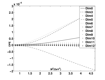
Figure 1: The various dimension OPE contribution as a function of $M^{2}$ in sum rule (4) for $\sqrt{s_{0}}=2.8~{}\mbox{GeV}$ for the scalar-scalar case with $\rho=1$.

Taking the scalar-scalar case as an example, its different dimension OPE contributions are compared as a function of $M^{2}$ in FIG. 1. Graphically, one can see that there are three main condensate contributions, i.e. the dimension $3$ two-quark condensate, the dimension $5$ mixed condensate, and the dimension $6$ four-quark condensate. These condensates could play an important role on the OPE side. The direct consequence is that it is of difficulty to choose a so-called “conventional Borel window” namely strictly satisfying that the low dimension condensate should be bigger than the high dimension contribution. Coming to think of it, these main condensates could cancel each other out to some extent. Meanwhile, most of other high dimension condensates involved are very small, for which can not radically influence the character of OPE convergence. All of these factors make that the perturbative term could play an important role on the total OPE contribution and the convergence of OPE is still under control at the relatively low value of $M^{2}$, and the lower bound of $M^{2}$ is taken as $0.8~{}\mbox{GeV}^{2}$ for this case.

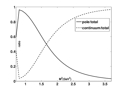
Figure 2: The phenomenological contribution in sum rule (4) for $\sqrt{s_{0}}=2.8~{}\mbox{GeV}$ for the scalar-scalar case with $\rho=1$. The solid line is the relative pole contribution (the pole contribution divided by the total, pole plus continuum contribution) as a function of $M^{2}$ and the dashed line is the relative continuum contribution.

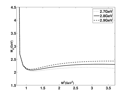
Figure 3: The mass of $0^{+}$ tetraquark state with the scalar-scalar configuration as a function of $M^{2}$ from sum rule (5) with $\rho=1$. The continuum thresholds are taken as $\sqrt{s_{0}}=2.7\sim 2.9~{}\mbox{GeV}$. The ranges of $M^{2}$ are $0.8\sim 1.5~{}\mbox{GeV}^{2}$ for $\sqrt{s_{0}}=2.7~{}\mbox{GeV}$, $0.8\sim 1.6~{}\mbox{GeV}^{2}$ for $\sqrt{s_{0}}=2.8~{}\mbox{GeV}$, and $0.8\sim 1.7~{}\mbox{GeV}^{2}$ for $\sqrt{s_{0}}=2.9~{}\mbox{GeV}$.

In the phenomenological side, a comparison between pole contribution and continuum contribution of sum rule (4) for the threshold $\sqrt{s_{0}}=2.8~{}\mbox{GeV}$ is shown in FIG. 2, which manifests that the relative pole contribution is about $50\%$ at $M^{2}=1.6~{}\mbox{GeV}^{2}$ and decreases with $M^{2}$. In a similar way, the upper bounds of Borel parameters are $M^{2}=1.5~{}\mbox{GeV}^{2}$ for $\sqrt{s_{0}}=2.7~{}\mbox{GeV}$ and $M^{2}=1.7~{}\mbox{GeV}^{2}$ for $\sqrt{s_{0}}=2.9~{}\mbox{GeV}$. Thereby, Borel windows for the scalar-scalar case are taken as $0.8\sim 1.5~{}\mbox{GeV}^{2}$ for $\sqrt{s_{0}}=2.7~{}\mbox{GeV}$, $0.8\sim 1.6~{}\mbox{GeV}^{2}$ for $\sqrt{s_{0}}=2.8~{}\mbox{GeV}$, and $0.8\sim 1.7~{}\mbox{GeV}^{2}$ for $\sqrt{s_{0}}=2.9~{}\mbox{GeV}$. In FIG. 3, the mass value $M_{H}$ as a function of $M^{2}$ from sum rule (5) for the scalar-scalar case is shown and one can visually see that there are indeed stable Borel plateaus. In the chosen work windows, $M_{H}$ is calculated to be $2.37\pm 0.33~{}\mbox{GeV}$. Furthermore, in view of the uncertainty due to the variation of quark masses and condensates, we have $2.37\pm 0.33^{+0.17}_{-0.03}~{}\mbox{GeV}$ (the first error is resulted from the variation of $\sqrt{s_{0}}$ and $M^{2}$, and the second error reflects the uncertainty rooting in the variation of QCD parameters) or briefly $2.37^{+0.50}_{-0.36}~{}\mbox{GeV}$ for the scalar-scalar tetraquark state.

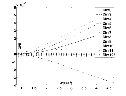
Figure 4: The various dimension OPE contribution as a function of $M^{2}$ in sum rule (4) for $\sqrt{s_{0}}=2.8~{}\mbox{GeV}$ for the axial-axial case with $\rho=1$.

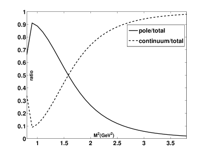
Figure 5: The phenomenological contribution in sum rule (4) for $\sqrt{s_{0}}=2.8~{}\mbox{GeV}$ for the axial-axial case with $\rho=1$. The solid line is the relative pole contribution (the pole contribution divided by the total, pole plus continuum contribution) as a function of $M^{2}$ and the dashed line is the relative continuum contribution.

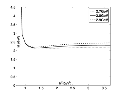
Figure 6: The mass of $0^{+}$ tetraquark state with the axial-axial configuration as a function of $M^{2}$ from sum rule (5) with $\rho=1$. The continuum thresholds are taken as $\sqrt{s_{0}}=2.7\sim 2.9~{}\mbox{GeV}$. The ranges of $M^{2}$ are $0.9\sim 1.5~{}\mbox{GeV}^{2}$ for $\sqrt{s_{0}}=2.7~{}\mbox{GeV}$, $0.9\sim 1.6~{}\mbox{GeV}^{2}$ for $\sqrt{s_{0}}=2.8~{}\mbox{GeV}$, and $0.9\sim 1.7~{}\mbox{GeV}^{2}$ for $\sqrt{s_{0}}=2.9~{}\mbox{GeV}$.

For the axial-axial case, its OPE contribution in sum rule (4) for $\sqrt{s_{0}}=2.8~{}\mbox{GeV}$ is shown in Fig. 4 by comparing various dimension contributions. Similarly, the dimension $3$, $5$, and $6$ condensates could cancel each other out to some extent and most of other dimension condensates are very small. On the other hand, the phenomenological contribution in sum rule (4) for $\sqrt{s_{0}}=2.8~{}\mbox{GeV}$ is pictured in Fig. 5. Eventually, work windows for the axial-axial case are chosen as $0.9\sim 1.5~{}\mbox{GeV}^{2}$ for $\sqrt{s_{0}}=2.7~{}\mbox{GeV}$, $0.9\sim 1.6~{}\mbox{GeV}^{2}$ for $\sqrt{s_{0}}=2.8~{}\mbox{GeV}$, and $0.9\sim 1.7~{}\mbox{GeV}^{2}$ for $\sqrt{s_{0}}=2.9~{}\mbox{GeV}$. The corresponding Borel curves for the axial-axial case are displayed in FIG. 6 and its mass is evaluated to be $2.51\pm 0.41~{}\mbox{GeV}$ in the chosen work windows. With an eye to the uncertainty from the variation of quark masses and condensates, for the axial-axial tetraquark state we achieve $2.51\pm 0.41^{+0.20}_{-0.02}~{}\mbox{GeV}$ (the first error reflects the uncertainty from the variation of $\sqrt{s_{0}}$ and $M^{2}$, and the second error roots in the variation of QCD parameters) or shortly $2.51^{+0.61}_{-0.43}~{}\mbox{GeV}$.

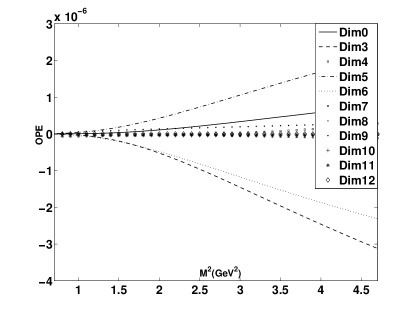
Figure 7: The various dimension OPE contribution as a function of $M^{2}$ in sum rule (4) for $\sqrt{s_{0}}=2.8~{}\mbox{GeV}$ for the pseudoscalar-pseudoscalar case with $\rho=1$.

For the pseudoscalar-pseudoscalar case, its various dimension OPE contribution in sum rule (4) for $\sqrt{s_{0}}=2.8~{}\mbox{GeV}$ is shown in Fig. 7. One may see that there are also three main condensates, i.e. the dimension $3$, $5$, and $6$ condensates. However, what apparently distinct from the foregoing two cases is that two main condensates (i.e. the dimension $3$ and $6$ condensates) have a different sign comparing to the perturbative term, which leads that the perturbative part and the total OPE even have different signs at length. The dissatisfactory OPE property causes that related Borel curves are rather unstable visually, and it is difficult to find reasonable work windows for this case. Accordingly, it is not advisable to continue extracting a numerical result.

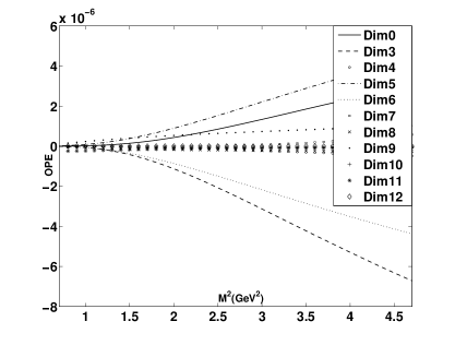
Figure 8: The various dimension OPE contribution as a function of $M^{2}$ in sum rule (4) for $\sqrt{s_{0}}=2.8~{}\mbox{GeV}$ for the vector-vector case with $\rho=1$.

For the vector-vector case, its different dimension OPE contribution in sum rule (4) for $\sqrt{s_{0}}=2.8~{}\mbox{GeV}$ is shown in Fig. 8. There appears the analogous problem as the pseudoscalar-pseudoscalar case, and the most direct consequence is that corresponding Borel curves are quite unstable. Hence it is hard to find appropriate work windows to grasp an authentic mass value for the vector-vector case.

II.4 numerical analysis with $\rho=3$ and other discussions

From the analysis in part C, one could see that high-dimension condensates have been included in the OPE to improve the $M^{2}$-stability of the sum rules. It is needed to point out that the included condensates are a part of more general condensate contributions at a given dimension. There is another source of uncertainty in the numerical results. Namely for the $d=6$ four-quark condensate, a general factorization $\langle\bar{q}q\bar{q}q\rangle=\rho\langle\bar{q}q\rangle^{2}$ has been hotly discussed in the past A ; B , where $\rho$ is a constant, which may be equal to $1$, to $2$, or be even smaller than $1$. (In particular, in Ref. C it is argued that this factorization may not happen at all.) Furthermore, there may be a poor quantitative control of the four-quark condensate due to the violation of factorization parameter which could be about $\rho=3\sim 4$ D . This feature indicates that the error quoted in the final result which does not take into account such a violation may be underestimated. Therefore, it is very necessary to investigate the effect of the factorization breaking.

Compromisingly, in this part we set $\rho=3$ for the $\langle\bar{q}q\bar{q}q\rangle=\rho\langle\bar{q}q\rangle^{2}$ factorization. Thus, there will be a factor $3$ for the four-quark condensate $\langle\bar{q}q\rangle^{2}$ and for the related classes of these high-dimension condensates (i.e. $\langle\bar{q}q\rangle^{3}$, $\langle\bar{q}q\rangle^{2}\langle g\bar{q}\sigma\cdot Gq\rangle$, $\langle\bar{q}q\rangle^{2}\langle g^{2}G^{2}\rangle$, and $\langle\bar{q}q\rangle^{2}\langle g^{3}G^{3}\rangle$) in the OPE side. From the similar analysis process as above, the relevant working windows for the scalar-scalar case are taken as: $M^{2}=0.9\sim 1.9~{}\mbox{GeV}^{2}$ for $\sqrt{s_{0}}=2.7~{}\mbox{GeV}$, $M^{2}=0.9\sim 2.0~{}\mbox{GeV}^{2}$ for $\sqrt{s_{0}}=2.8~{}\mbox{GeV}$, and $M^{2}=0.9\sim 2.1~{}\mbox{GeV}^{2}$ for $\sqrt{s_{0}}=2.9~{}\mbox{GeV}$. The Borel curves for this case are shown in FIG. 9 and in the chosen windows its mass is computed to be $2.23\pm 0.18~{}\mbox{GeV}$. Considering uncertainty due to the variation of quark masses and condensates, one can achieve the final result $2.23^{+0.78}_{-0.24}~{}\mbox{GeV}$.

Similarly, with $\rho=3$ the working windows for the axial-axial case are taken as: $M^{2}=0.9\sim 1.8~{}\mbox{GeV}^{2}$ for $\sqrt{s_{0}}=2.7~{}\mbox{GeV}$, $M^{2}=0.9\sim 1.9~{}\mbox{GeV}^{2}$ for $\sqrt{s_{0}}=2.8~{}\mbox{GeV}$, and $M^{2}=0.9\sim 2.0~{}\mbox{GeV}^{2}$ for $\sqrt{s_{0}}=2.9~{}\mbox{GeV}$. The corresponding Borel curves are shown in FIG. 10 and its mass is evaluated to be $2.52\pm 0.47~{}\mbox{GeV}$ in the work windows. With a view to uncertainty due to the variation of quark masses and condensates, we have the eventual result $2.52^{+0.76}_{-0.52}~{}\mbox{GeV}$.

By this time, note that the $m_{c}$ value is taken as the running charm quark mass $1.27\pm 0.03~{}\mbox{GeV}$, which is often used in the existing literature. Without any evaluation of the perturbation theory radiative corrections, one can equally use the pole mass $M_{c}\doteq 1.4\sim 1.5~{}\mbox{GeV}$ D . One should take into account a such ambiguity of the charm quark mass definition to clarify the effects on numerical results for the choice of mass (running or pole). After setting $\rho=3$, replacing the charm running mass by the pole mass, and carrying on the same analysis process as above, one can obtain the mass ranges $2.11\sim 3.16~{}\mbox{GeV}$ for the scalar-scalar configuration and $2.11\sim 4.31~{}\mbox{GeV}$ for the axial-axial case.

Additionally, the way to construct a scalar out of two axial-vector currents or two vector currents could be not unique. In general, when one combines two spin $1$ currents one may obtain states with spin = $0$, $1$ and $2$. To be sure that one is dealing with a scalar, it is needed to project the combination of the currents into the spin $0$ channel, which can be done with the help of the projection operators E . Since the direct contraction used here contains the overlap with the rigorous projection, the results found in this work can be close enough to the projection disposal. Certainly, one should note that on the final results there may exist the source of uncertainty from different treatments of currents.

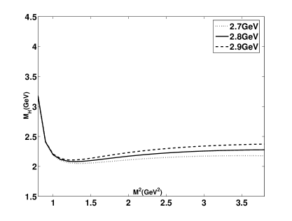
Figure 9: The mass of $0^{+}$ tetraquark state with the scalar-scalar configuration as a function of $M^{2}$ from sum rule (5) with $\rho=3$. The continuum thresholds are taken as $\sqrt{s_{0}}=2.7\sim 2.9~{}\mbox{GeV}$. The ranges of $M^{2}$ are $0.9\sim 1.9~{}\mbox{GeV}^{2}$ for $\sqrt{s_{0}}=2.7~{}\mbox{GeV}$, $0.9\sim 2.0~{}\mbox{GeV}^{2}$ for $\sqrt{s_{0}}=2.8~{}\mbox{GeV}$, and $0.9\sim 2.1~{}\mbox{GeV}^{2}$ for $\sqrt{s_{0}}=2.9~{}\mbox{GeV}$.

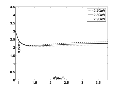
Figure 10: The mass of $0^{+}$ tetraquark state with the axial-axial configuration as a function of $M^{2}$ from sum rule (5) with $\rho=3$. The continuum thresholds are taken as $\sqrt{s_{0}}=2.7\sim 2.9~{}\mbox{GeV}$. The ranges of $M^{2}$ are $0.9\sim 1.8~{}\mbox{GeV}^{2}$ for $\sqrt{s_{0}}=2.7~{}\mbox{GeV}$, $0.9\sim 1.9~{}\mbox{GeV}^{2}$ for $\sqrt{s_{0}}=2.8~{}\mbox{GeV}$, and $0.9\sim 2.0~{}\mbox{GeV}^{2}$ for $\sqrt{s_{0}}=2.9~{}\mbox{GeV}$.

III Summary

Triggered by the new observation of $D_{s0}^{*}(2317)$ by BESIII Collaboration, we investigate that whether $D_{s0}^{*}(2317)$ could be a $0^{+}$ tetraquark state employing QCD sum rules. In order to insure the quality of sum rule analysis, contributions of condensates up to dimension $12$ have been computed to test the OPE convergence. We find that some condensates, i.e. the two-quark condensate, the mixed condensate, and the four-quark condensate are of importance to the OPE side. Not bad for the scalar-scalar and the axial-axial cases, their main condensates could cancel each other out to some extent. Most of other condensates calculated are very small, which means that they could not radically influence the character of OPE convergence. All these factors bring that the OPE convergence for the scalar-scalar and the axial-axial cases is still controllable.

To the end, we gain the following results: firstly, the final result for the scalar-scalar case is $2.37^{+0.50}_{-0.36}~{}\mbox{GeV}$ with the factorization parameter $\rho=1$ (or $2.23^{+0.78}_{-0.24}~{}\mbox{GeV}$ with $\rho=3$), which is in good agreement with the experimental value of $D_{s0}^{*}(2317)$. This result supports that $D_{s0}^{*}(2317)$ could be deciphered as a $0^{+}$ tetraquark state with the scalar-scalar configuration. Secondly, the eventual result for the axial-axial case is $2.51^{+0.61}_{-0.43}~{}\mbox{GeV}$ with $\rho=1$ (or $2.52^{+0.76}_{-0.52}~{}\mbox{GeV}$ with $\rho=3$), which is still coincident with the data of $D_{s0}^{*}(2317)$ considering the uncertainty although its central value is somewhat higher. In this way, one could not preclude the possibility of $D_{s0}^{*}(2317)$ as an axial-axial configuration tetraquark state. Meanwhile, one should note the weakness of convergence in the OPE side while presenting these results. Thirdly, the obtained mass ranges are $2.11\sim 3.16~{}\mbox{GeV}$ for the scalar-scalar configuration and $2.11\sim 4.31~{}\mbox{GeV}$ for the axial-axial case while setting $\rho=3$ and taking the charm pole mass, which are both in accord with the experimental value of $D_{s0}^{*}(2317)$. Fourthly, the OPE convergence is so unsatisfying for the pseudoscalar-pseudoscalar and the vector-vector cases that one can not find appropriate work windows to acquire reliable hadronic information for these two cases.

In the future, with more data accumulated at BESIII or a fine scan from PANDA PANDA , experimental observations may shed more light on the nature of $D_{s0}^{*}(2317)$. Besides, one can also expect that the inner structure of $D_{s0}^{*}(2317)$ could be further uncovered by continuously theoretical efforts.

- (1) M. Ablikim et al. (BESIII Collaboration), Phys. Rev. D 97, 051103 (2018).
- (2) B. Aubert et al. (BABAR Collaboration), Phys. Rev. Lett. 90, 242001 (2003).
- (3) B. Aubert et al. (BABAR Collaboration), Phys. Rev. Lett. 93, 181801 (2004).
- (4) D. Besson et al. (CLEO Collaboration), Phys. Rev. D 68, 032002 (2003).
- (5) P. Krokovny et al. (Belle Collaboration), Phys. Rev. Lett. 91, 262002 (2003).
- (6) P. Colangelo and F. De Fazio, Phys. Lett. B 570, 180 (2003); P. Colangelo, F. De Fazio, and A. Ozpineci, Phys. Rev. D 72, 074004 (2005).
- (7) S. Godfrey and N. Isgur, Phys. Rev. D 32, 189 (1985); S. Godfrey and R. Kokoski, Phys. Rev. D 43, 1679 (1991); J. Zeng, J. W. Van Orden, and W. Roberts, Phys. Rev. D 52, 5229 (1995); D. Ebert, V. O. Galkin, and R. N. Faustov, Phys. Rev. D 57, 5663 (1998); Y. S. Kalashnikova, A. V. Nefediev, and Y. A. Simonov, Phys. Rev. D 64, 014037 (2001); M. Di Pierro and E. Eichten, Phys. Rev. D 64, 114004 (2001).
- (8) G. S. Bali, Phys. Rev. D 68, 071501 (2003); A. Dougall, R. D. Kenway, C. M. Maynard, and C. McNeile (UKQCD Collaboration), Phys. Lett. B 569, 41 (2003).
- (9) S. Godfrey, Phys. Lett. B 568, 254 (2003).
- (10) T. Barnes, F. E. Close, and H. J. Lipkin, Phys. Rev. D 68, 054006 (2003); E. E. Kolomeitsev and M. F. M. Lutz, Phys. Lett. B 582, 39 (2004); F. K. Guo, P. N. Shen, H. C. Chiang, R. G. Ping, and B. S. Zou, Phys. Lett. B 641, 278 (2006); A. Faessler, T. Gutsche, V. E. Lyubovitskij, and Y. L. Ma, Phys. Rev. D 76, 014005 (2007); D. Gamermann, E. Oset, D. Strottman, and M. J. Vicente Vacas, Phys. Rev. D 76, 074016 (2007); F. K. Guo, C. Hanhart, and U. G. Meissner, Eur. Phys. J. A 40, 171 (2009); M. Cleven, F. K. Guo, C. Hanhart, and U. G. Meissner, Eur. Phys. J. A 47, 19 (2011).
- (11) H. Y. Cheng and W. S. Hou, Phys. Lett. B 566, 193 (2003); Y. Q. Chen and X. Q. Li, Phys. Rev. Lett. 93, 232001 (2004); V. Dmitrasinovic, Phys. Rev. Lett. 94, 162002 (2005).
- (12) E. V. Beveran and G. Rupp, Phys. Rev. Lett. 91, 012003 (2003); K. Terasaki, Phys. Rev. D 68, 011501 (2003); T. E. Browder, S. Pakvasa, and A. A. Petrov, Phys. Lett. B 578, 365 (2004); L. Maiani, F. Piccinini, A. D. Polosa, and V. Riquer, Phys. Rev. D 71, 014028 (2005); L. Liu, K. Orginos, F. K. Guo, C. Hanhart, and U. G. Meissner, Phys. Rev. D 87, 014508 (2013); D. Mohler, C. B. Lang, L. Leskovec, S. Prelovsek, and R. M. Woloshyn, Phys. Rev. Lett. 111, 222001 (2013); C. B. Lang, L. Leskovec, D. Mohler, S. Prelovsek, and R. M. Woloshyn, Phys. Rev. D 90, 034510 (2014).
- (13) M. A. Shifman, A. I. Vainshtein, and V. I. Zakharov, Nucl. Phys. B147, 385 (1979); B147, 448 (1979); V. A. Novikov, M. A. Shifman, A. I. Vainshtein, and V. I. Zakharov, Fortschr. Phys. 32, 585 (1984).
- (14) B. L. Ioffe, in The Spin Structure of The Nucleon, edited by B. Frois, V. W. Hughes, and N. de Groot (World Scientific, Singapore, 1997).
- (15) S. Narison, Camb. Monogr. Part. Phys. Nucl. Phys. Cosmol. 17, 1 (2002).
- (16) P. Colangelo and A. Khodjamirian, in At the Frontier of Particle Physics: Handbook of QCD, edited by M. Shifman, Boris Ioffe Festschrift Vol. 3 (World Scientific, Singapore, 2001), pp. 1495-1576.
- (17) L. J. Reinders, H. R. Rubinstein, and S. Yazaki, Phys. Rep. 127, 1 (1985).
- (18) M. Nielsen, F. S. Navarra, and S. H. Lee, Phys. Rep. 497, 41 (2010).
- (19) Y. B. Dai, C. S. Huang, C. Liu, and S. L. Zhu, Phys. Rev. D 68, 114011 (2003).
- (20) M. Q. Huang, Phys. Rev. D 69, 114015 (2004).
- (21) S. Narison, Phys. Lett. B 605, 319 (2005).
- (22) A. Hayashigaki and K. Terasaki, arXiv:0411285 [hep-ph].
- (23) Z. G. Wang and S. L. Wan, Phys. Rev. D 73, 094020 (2006).
- (24) Y. B. Dai, X. Q. Li, S. L. Zhu, and Y. B. Zuo, Eur. Phys. J. C 55, 249 (2008).
- (25) H. Y. Jin, J. Zhang, Z. F. Zhang, and T. G. Steele, Phys. Rev. D 81, 054021 (2010).
- (26) E. V. Veliev and G. Kaya, Acta Phys. Polon. B 41, 1905 (2010).
- (27) Z. G. Wang and S. L. Wan, Nucl. Phys. A 778, 22 (2006).
- (28) M. E. Bracco, A. Lozea, R. D. Matheus, F. S. Navarra, and M. Nielsen, Phys. Lett. B 624, 217 (2005).
- (29) H. Kim and Y. Oh, Phys. Rev. D 72, 074012 (2005).
- (30) W. Chen, H. X. Chen, X. Liu, T. G. Steele, and S. L. Zhu, Phys. Rev. D 95, 114005 (2017).
- (31) H. X. Chen, A. Hosaka, and S. L. Zhu, Phys. Lett. B 650, 369 (2007).
- (32) Z. G. Wang, Nucl. Phys. A 791, 106 (2007).
- (33) R. D. Matheus, F. S. Navarra, M. Nielsen, and R. Rodrigues da Silva, Phys. Rev. D 76, 056005 (2007).
- (34) J. R. Zhang, L. F. Gan, and M. Q. Huang, Phys. Rev. D 85, 116007 (2012); J. R. Zhang and G. F. Chen, Phys. Rev. D 86, 116006 (2012); J. R. Zhang, Phys. Rev. D 87, 076008 (2013); Phys. Rev. D 89, 096006 (2014).
- (35) J. R. Zhang and M. Q. Huang, Phys. Rev. D 77, 094002 (2008); JHEP 1011, 057 (2010); Phys. Rev. D 83, 036005 (2011).
- (36) J. R. Zhang, J. L. Zou, and J. Y. Wu, Chin. Phys. C 42, 043101 (2018).
- (37) C. Patrignani et al. (Particle Data Group), Chin. Phys. C 40, 100001 (2016).
- (38) S. Narison, Phys. Rep. 84, 263 (1982); G. Launer, S. Narison, and R. Tarrach, Z. Phys. C 26, 433 (1984); S. Narison, Riv. Nuovo Cimento 10N2, 1 (1987); S. Narison, World Sci. Lecture Notes Phys. 26, 1 (1989); S. Narison, Acta Phys. Polon. 26, 687 (1995); S. Narison, Phys. Lett. B 673, 30 (2009).
- (39) R. Thomas, T. Hilger, and B. Kämpfer, Nucl. Phys. A 795, 19 (2007); A. Gómez Nicola, J. R. Peláez, and J. Ruiz de Elvira, Phys. Rev. D 82, 074012 (2010); H. S. Zong, D. K. He, F. Y. Hou, and W. M. Sun, Int. J. Mod. Phys. A 23, 1507 (2008); S. Narison, Phys. Lett. B 707, 259 (2012).
- (40) F. L. Braghin and F. S. Navarra, arXiv:1404.4094 [hep-ph], Phys. Rev. D 91, 074008 (2015).
- (41) R. Albuquerque, S. Narison, A. Rabemananjara, and D. Rabetiarivony, Int. J. Mod. Phys. A 31, 1650093 (2016); R. Albuquerque, S. Narison, F. Fanomezana, A. Rabemananjara, D. Rabetiarivony, and G. Randriamanatrika, Int. J. Mod. Phys. A 31, 1650196 (2016); R. Albuquerque, S. Narison, D. Rabetiarivony, and G. Randriamanatrika, arXiv:1801.03073 [hep-ph].
- (42) A. Martínez Torres, K. P. Khemchandani, M. Nielsen, F. S. Navarra, and E. Oset, Phys. Rev. D 88, 074033 (2013); K. P. Khemchandani, A. Martínez Torres, M. Nielsen, and F. S. Navarra, Phys. Rev. D 89, 014029 (2014); A. Martínez Torres, K. P. Khemchandani, J. M. Dias, F. S. Navarra, and M. Nielsen, Nucl. Phys. A 966, 135 (2017).
- (43) E. Prencipe et al. (PANDA Collaboration), EPJ Web Conf. 95, 04052 (2015).