Satisfiability Modulo Transcendental Functions via Incremental Linearization

Abstract

In this paper we present an abstraction-refinement approach to Satisfiability Modulo the theory of transcendental functions, such as exponentiation and trigonometric functions. The transcendental functions are represented as uninterpreted in the abstract space, which is described in terms of the combined theory of linear arithmetic on the rationals with uninterpreted functions, and are incrementally axiomatized by means of upper- and lower-bounding piecewise-linear functions. Suitable numerical techniques are used to ensure that the abstractions of the transcendental functions are sound even in presence of irrationals. Our experimental evaluation on benchmarks from verification and mathematics demonstrates the potential of our approach, showing that it compares favorably with delta-satisfiability/interval propagation and methods based on theorem proving.

1 Introduction

Many applications require dealing with transcendental functions (e.g., exponential, logarithm, sine, cosine). Nevertheless, the problem of Satisfiability Modulo the theory of transcendental functions comes with many difficulties. First, the problem is in general undecidable [22]. Second, we may be forced to deal with irrational numbers - in fact, differently from polynomial, transcendental functions most often have irrational values for rational arguments. (See, for example, Hermite’s proof that $\exp(x)$ is irrational for rational non-zero $x$.)

In this paper, we describe a novel approach to Satisfiability Modulo the quantifier-free theory of (nonlinear arithmetic with) transcendental functions over the reals - SMT(NTA). The approach is based on an abstraction-refinement loop, using SMT(UFLRA) as abstract space, UFLRA being the combined theory of linear arithmetic on the rationals with uninterpreted functions. The Uninterpreted Functions are used to model nonlinear and transcendental functions. Then, we iteratively incrementally axiomatize the transcendental functions with a lemma-on-demand approach. Specifically, we eliminate spurious interpretations in SMT(UFLRA) by tightening the piecewise-linear envelope around the (uninterpreted counterpart of) the transcendental functions.

A key challenge is to compute provably correct approximations, also in presence of irrational numbers. We use Taylor series to exactly compute suitable accurate rational coefficients. We remark that nonlinear polynomials are only used to numerically compute the coefficients –i.e., no SMT solving in the theory of nonlinear arithmetic (SMT(NRA)) is needed– whereas the refinement is based on the addition, in the abstract space, of piecewise-linear axiom instantiations, which upper- and lower-bound the candidate solutions, ruling out spurious interpretations. To compute such piecewise-linear bounding functions, the concavity of the curve is taken into account. In order to deal with trigonometric functions, we take into account the periodicity, so that the axiomatization is only done in the interval between $-\pi$ and $\pi$. Interestingly, not only this is helpful for efficiency, but also it is required to ensure correctness.

Another distinguishing feature of our approach is a logical method to conclude the existence of a solution without explicitly constructing it. We use a sufficient criterion that consists in checking whether the formula is satisfiable under all possible interpretations of the uninterpreted functions (representing the transcendental functions) that are consistent with some rational interval bounds within which the correct values for the transcendental functions are guaranteed to exist. We encode the problem as a SMT(UFLRA) satisfiability check, such that an unsatisfiable result implies the satisfiability of the original SMT(NTA) formula.

We implemented the approach on top of the MathSAT SMT solver [7], using the PySMT library [14]. We experimented with benchmarks from SMT-based verification queries over nonlinear transition systems, including Bounded Model Checking of hybrid automata, as well as from several mathematical properties from the MetiTarski [1] suite and from other competitor solver distributions. We contrasted our approach with state-of-the-art approaches based on interval propagation (iSAT3 and dReal), and with the deductive approach in MetiTarski. The results show that our solver compares favourably with the other solvers, being able to decide the highest number of benchmarks.

This paper is organized as follows. In §2 we describe some background. In §3 we overview the approach, defining the foundation for safe linear approximations. In §4 we describe the specific axiomatization for transcendental functions. In §5 we discuss the related literature, and in §6 we present the experimental evaluation. In §7 we draw some conclusions and outline directions for future work.

2 Background

We assume the standard first-order quantifier-free logical setting and standard notions of theory, satisfiability, and logical consequence. As usual in SMT, we denote with LRA the theory of linear real arithmetic, with NRA that of non-linear real arithmetic, with UF the theory of equality (with uninterpreted functions), and with UFLRA the combined theory of UF and LRA. Unless otherwise specified, we use the terms variable and free constant interchangeably. We denote formulas with $\varphi,\psi$, terms with $t$, variables with $x,y,a,b$, functions with $f,\mathop{t\!f},\mathop{f\!t\!f}$, each possibly with subscripts. If $x$ and $y$ are two variables, we denote with $\varphi{\{x\mapsto y\}}$ the formula obtained by replacing all the occurrences of $x$ in $\varphi$ with $y$. We extend this notation to ordered sequences of variables in the natural way. If $\mu$ is a model and $x$ is a variable, we write $\mu[x]$ to denote the value of $x$ in $\mu$, and we extend this notation to terms and formulas in the usual way. If $\Gamma$ is a set of formulas, we write $\bigwedge\Gamma$ to denote the formula obtained by taking the conjunction of all its elements. We write $t_{1}<t_{2}<t_{3}$ for $t_{1}<t_{2}\wedge t_{2}<t_{3}$.

A transcendental function is an analytic function that does not satisfy a polynomial equation (in contrast to an algebraic function [26, 15]). Within this paper we consider univariate exponential, logarithmic, and trigonometric functions. We denote with NTA the theory of (non-linear) real arithmetic extended with these transcendental functions.

A tangent line to a univariate function $f(x)$ at a point of interest $x=a$ is a straight line that “just touches” the function at the point, and represents the instantaneous rate of change of the function $f$ at that one point. The tangent line $T_{f,a}(x)$ to the function $f$ at point $a$ is the straight line defined as follows:

$$T_{f,a}(x)\stackrel{{\scriptstyle\text{\tiny def}}}{{=}}f(a)+\frac{d}{dx}f(a)*(x-a)$$

where $\frac{d}{dx}f$ is the first-order derivative of $f$ wrt. $x$.

A secant line to a univariate function $f(x)$ is a straight line that connects two points on the function plot. The secant line $S_{f,a,b}(x)$ to a function $f$ between points $a$ and $b$ is defined as follows:

$$S_{f,a,b}(x)\stackrel{{\scriptstyle\text{\tiny def}}}{{=}}\frac{f(a)-f(b)}{a-b}*(x-a)+f(a).$$

For a function $f$ that is twice differentiable at point $c$, the concavity of $f$ at $c$ is the sign of its second derivative evaluated at $c$. We denote open and closed intervals between two real numbers $l$ and $u$ as $]l,u[$ and $[l,u]$ respectively. Given a univariate function $f$ over the reals, the graph of $f$ is the set of pairs $\{\langle x,f(x)\rangle~{}|~{}x\in\mathbb{R}\}$. We might sometimes refer to an element $\langle x,f(x)\rangle$ of the graph as a point.

Taylor Series and Taylor’s Theorem.

Given a function $f(x)$ that has $n+1$ continuous derivatives at $x=a$, the Taylor series of degree $n$ centered around $a$ is the polynomial:

$$P_{n,f(a)}(x)\stackrel{{\scriptstyle\text{\tiny def}}}{{=}}\sum_{i=0}^{n}\frac{f^{(i)}(a)}{i!}*(x-a)^{i}$$

where $f^{(i)}(a)$ is the evaluation of $i$-th derivative of $f(x)$ at point $x=a$. The Taylor series centered around $0$ is also called Maclaurin series.

According to Taylor’s theorem, any continuous function $f(x)$ that is $n+1$ differentiable can be written as the sum of the Taylor series and the remainder term:

$$f(x)=P_{n,f(a)}(x)+R_{n+1,f(a)}(x)$$

where $R_{n+1,f(a)}(x)$ is basically the Lagrange form of the remainder, and for some point $b$ between $x$ and $a$ it is given by:

$$R_{n+1,f(a)}(x)\stackrel{{\scriptstyle\text{\tiny def}}}{{=}}\frac{f^{(n+1)}(b)}{(n+1)!}*(x-a)^{n+1}.$$

The value of the point $b$ is not known, but the upper bound on the size of the remainder $\overline{R_{n+1,f(a)}}^{\;u}(x)$ at a point $x$ can be estimated by:

$$\overline{R_{n+1,f(a)}}^{\;u}(x)\stackrel{{\scriptstyle\text{\tiny def}}}{{=}}\max_{c\in[\min(a,x),\max(a,x)]}(|f^{(n+1)}(c)|)*\frac{|(x-a)^{n+1}|}{(n+1)!}.$$

This allows to obtain two polynomials that are above and below the function at a given point $x$, by considering $P_{n,f(a)}(x)+\overline{R_{n+1,f(a)}}^{\;u}(x)$ and $P_{n,f(a)}(x)-\overline{R_{n+1,f(a)}}^{\;u}(x)$ respectively.

3 Overview of the approach

bool SMT-NTA-check-abstract ($\varphi$): 1.   $\widehat{\varphi}=\textsf{\scalebox{0.9}{initial-abstraction}}(\varphi)$ 2.   $\Gamma=\emptyset$ 3.   precision := initial-precision () 4.   while true: 5. if budget-exhausted (): 6. abort 7. $\langle res,\widehat{\mu}\rangle$ = SMT-UFLRA-check ($\widehat{\varphi}\land\bigwedge\Gamma$) 8. if not res: 9. return false 10. $\langle sat,\Gamma^{\prime}\rangle$ := check-refine ($\varphi$, $\widehat{\mu}$, precision) 11. if sat: 12. return true 13. else: 14. precision := maybe-increase-precision () 15. $\Gamma^{\prime\prime}$ := refine-extra ($\varphi$, $\widehat{\mu}$) 16. $\Gamma$ := $\Gamma\cup\Gamma^{\prime}\cup\Gamma^{\prime\prime}$

Figure 1: Solving SMT(NTA) via abstraction to SMT(UFLRA).

Our procedure, which extends to SMT(NTA) and pushes further the approach presented in [5] for SMT(NRA), works by overapproximating the input formula with a formula over the combined theory of linear arithmetic and uninterpreted functions. The main algorithm is shown in Fig. 1. The solving procedure follows a classic abstraction-refinement loop, in which at each iteration, the current safe approximation $\widehat{\varphi}$ of the input SMT(NTA) formula $\varphi$ is refined by adding new constraints $\Gamma$ that rule out one (or possibly more) spurious solutions, until one of the following conditions occurs: (i) the resource budget (e.g. time, memory, number of iterations) is exhausted; or (ii) $\widehat{\varphi}\land\bigwedge\Gamma$becomes unsatisfiable in SMT(UFLRA); or (iii) the SMT(UFLRA) satisfiability result for $\widehat{\varphi}\land\bigwedge\Gamma$ can be lifted to a satisfiability result for the original formula $\varphi$. An initial current precision is set (calling the function initial-precision), and this value is possibly increased at each iteration (calling maybe-increase-precision) according to the result of check-refine and some heuristic.

In Fig. 1 we distinguish between two different refinement procedures: 1) check-refine, which is described below; 2) refine-extra, which is described in §4, where we provide further details on the treatment of each specific transcendental function that we currently support.

3.0.1 Initial Abstraction.

The function initial-abstraction takes in input an SMT(NTA) formula $\varphi$ and returns a SMT(UFLRA) safe approximation $\widehat{\varphi}$ of it. First, we flatten each transcendental function application $\mathop{t\!f}(t)$ in $\varphi$ in which $t$ is not a variable by replacing $t$ with a fresh variable $y$, and by conjoining $y=t$ to $\varphi$. Then, we replace each transcendental function $\mathop{t\!f}(x)$ in $\varphi$ with a corresponding uninterpreted function $\mathop{f\!t\!f}(x)$, producing thus an SMT(UFLRA) formula $\widehat{\varphi}$. Finally, we add to $\widehat{\varphi}$ some simple initial axioms for the different transcendental functions, expressing general, simple mathematical properties about them. We shall describe such axioms in §4.

If $\varphi$ contains also non-linear polynomials, we handle them as described in [5]: we replace each non-linear product $t_{1}*t_{2}$ with an uninterpreted function application $fmul(t_{1},t_{2})$, and add to the input formula some initial axioms expressing general, simple mathematical properties of multiplications. (We refer the reader to [5] for details.)

3.0.2 Spuriousness check and abstraction refinement.

$\langle{\bf bool},\text{axiom-set}\rangle$ check-refine ($\varphi$, $\widehat{\mu}$, precision): 1.    $\Gamma$ := check-refine-NRA ($\varphi$, $\widehat{\mu}$)  # NRA refinement of [5] 2.   $\epsilon$ := $10^{-\text{precision}}$ 3.    for all $\mathop{t\!f}(x)\in\varphi$: 4. $c$ := $\widehat{\mu}[x]$ 5. $\langle P_{l}(x),P_{u}(x)\rangle$ := poly-approx ($\mathop{t\!f}(x)$, $c$, $\epsilon$) 6. if $\widehat{\mu}[\mathop{f\!t\!f}(x)]\leq P_{l}(c)$ or $\widehat{\mu}[\mathop{f\!t\!f}(x)]\geq P_{u}(c)$: 7. $\Gamma$ := $\Gamma\cup$ get-lemmas-point ($\mathop{t\!f}(x)$, $\widehat{\mu}$, $P_{l}(x)$, $P_{u}(x)$) 8.   if $\Gamma=\emptyset$: 9. if check-model ($\varphi$, $\widehat{\mu}$): 10. return $\langle{\bf true},\emptyset\rangle$ 11. else: 12. return check-refine ($\varphi$, $\widehat{\mu}$, precision+1) 13.   else: 14. return $\langle{\bf false},\Gamma\rangle$

Figure 2: The main refinement procedure.

The core of our procedure is the check-refine function, shown in Fig. 2.

First, if the formula contains also some non-linear polynomials, check-refine performs the refinement of non-linear multiplications as described in [5]. In Fig. 2, this is represented by the call to the function check-refine-NRA at line 2, which may return some axioms to further constrain $fmul$ terms. If no non-linear polynomials occur in $\varphi$, then $\Gamma$ is initialized as the empty set.

Then, the function iterates over all the transcendental function applications $\mathop{t\!f}(x)$ in $\varphi$ (lines 2–2), and checks whether the SMT(UFLRA)-model $\widehat{\mu}$ is consistent with their semantics.

Intuitively, in principle, this amounts to check that $\mathop{t\!f}(\widehat{\mu}[x])$ is equal to $\widehat{\mu}[\mathop{f\!t\!f}(x)]$. In practice, however, the check cannot be exact, since transcendental functions at rational points typically have irrational values (see e.g. [21]), which cannot be represented in SMT(UFLRA). Therefore, for each $\mathop{t\!f}(x)$ in $\varphi$, we instead compute two polynomials, $P_{l}(x)$ and $P_{u}(x)$, with the property that $\mathop{t\!f}(\widehat{\mu}[x])$ belongs to the open interval $]P_{l}(\widehat{\mu}[x]),P_{u}(\widehat{\mu}[x])[$. The polynomials are computed using Taylor series, according to the given current precision, by the function poly-approx, which shall be described in §4.

If the model value $\widehat{\mu}[\mathop{f\!t\!f}(x)]$ for $\mathop{t\!f}(x)$ is outside the above interval, then the function get-lemmas-point is used to generate some linear lemmas that will remove the spurious point $\langle\widehat{\mu}[x],\widehat{\mu}[\mathop{f\!t\!f}(x)]\rangle$ from the graph of the current abstraction of $\mathop{t\!f}(x)$ (line 2).

If at least one point was refined in the loop of lines 2–2, the current set of lemmas $\Gamma$ is returned (line 2). If instead none of the points was determined to be spurious, the function check-model is called (line 2). This function tries to determine whether the abstract model $\widehat{\mu}$ does indeed imply the existence of a model for the original formula $\varphi$ (more details are given below). If the check fails, we repeat the check-refine call with an increased precision (line 2).

3.0.3 Refining a spurious point with secant and tangent lines.

axiom-set get-lemmas-point ($\mathop{t\!f}(x)$, $\widehat{\mu}$, $P_{l}(x)$, $P_{u}(x)$): 1.   $c$ := $\widehat{\mu}[x]$ 2.   $v$ := $\widehat{\mu}[\mathop{f\!t\!f}(x)]$ 3.   conc := get-concavity ($\mathop{t\!f}(x)$, $c$) 4.    if ($v\leq P_{l}(c)$ and $\text{conc}\geq 0$) or ($v\geq P_{u}(c)$ and $\text{conc}\leq 0$):   4.     # tangent refinement 5. $P$ := $(v\leq P_{l}(c))~{}?~{}(P_{l})~{}:~{}(P_{u})$ 6. $T(x)$ := $P(c)+\frac{d}{dx}P(c)\cdot(x-c)$  # tangent of $P$ at $c$ 7. $\langle l,u\rangle$ := get-tangent-bounds ($\mathop{t\!f}(x)$, $c$, $\frac{d}{dx}P(c)$) 8. $\psi$ := $(\text{conc}<0)~{}?~{}(\mathop{f\!t\!f}(x)\leq T(x))~{}:~{}(\mathop{f\!t\!f}(x)\geq T(x))$ 9. return {$((x\geq l)\land(x\leq u))\rightarrow\psi$} 10.    else:  # $(v\leq P_{l}(c)\land\text{conc}<0)\lor(v\geq P_{u}(c)\land\text{conc}>0)$   10.     # secant refinement 11. prev := get-previous-secant-points ($\mathop{t\!f}(x)$) 12. $l$ := $\text{max}\{p\in\text{prev}~{}|~{}p<c\}$ 13. $u$ := $\text{min}\{p\in\text{prev}~{}|~{}p>c\}$ 14. $P$ := $(v\leq P_{l}(c))~{}?~{}(P_{l})~{}:~{}(P_{u})$ 15. $S_{l}(x)$ := $\dfrac{P(l)-P(c)}{l-c}\cdot(x-l)+P(l)$  # secant of $P$ between $l$ and $c$ 16. $S_{u}(x)$ := $\dfrac{P(u)-P(c)}{u-c}\cdot(x-u)+P(u)$ 17. $\psi_{l}$ := $(\text{conc}<0)~{}?~{}(\mathop{f\!t\!f}(x)\geq S_{l}(x))~{}:~{}(\mathop{f\!t\!f}(x)\leq S_{l}(x))$ 18. $\psi_{u}$ := $(\text{conc}<0)~{}?~{}(\mathop{f\!t\!f}(x)\geq S_{u}(x))~{}:~{}(\mathop{f\!t\!f}(x)\leq S_{u}(x))$ 19. $\phi_{l}$ := $(x\geq l)\land(x\leq c)$ 20. $\phi_{u}$ := $(x\geq c)\land(x\leq u)$ 21. store-secant-point ($\mathop{t\!f}(x)$, $c$) 22. return {$(\phi_{l}\rightarrow\psi_{l})$, $(\phi_{u}\rightarrow\psi_{u})$}

Figure 3: Piecewise-linear refinement for the transcendental function $\mathop{t\!f}(x)$ at point $c$.

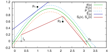
Figure 4: Piecewise-linear refinement illustration.

Given a transcendental function application $\mathop{t\!f}(x)$, the get-lemmas-point function generates a set of lemmas for refining the interpretation of $\mathop{f\!t\!f}(x)$ by constructing a piecewise-linear approximation of $\mathop{t\!f}(x)$ around the point $\widehat{\mu}[x]$, using one of the polynomials $P_{l}(x)$ and $P_{u}(x)$ computed in check-refine. The kind of lemmas generated, and which of the two polynomials is used, depend on (i) the position of the spurious value $\widehat{\mu}[\mathop{f\!t\!f}(x)]$ relative to the correct value $\mathop{t\!f}(\widehat{\mu}[x])$, and (ii) the concavity of $\mathop{t\!f}$ around the point $\widehat{\mu}[x]$. If the concavity is positive (resp. negative) or equal to zero, and the point lies below (resp. above) the function, then the linear approximation is given by a tangent to the lower (resp. upper) bound polynomial $P_{l}$ (resp. $P_{u}$) at $\widehat{\mu}[x]$ (lines 3–3 of Fig. 3); otherwise, i.e. the concavity is negative (resp. positive) and the point is below (resp. above) the function, the linear approximation is given by a pair of secants to the lower (resp. upper) bound polynomial $P_{l}$ (resp. $P_{u}$) around $\widehat{\mu}[x]$ (lines 3–3 of Fig. 3). The two situations are illustrated in Fig. 4.

In the case of tangent refinement, the function get-tangent-bounds (line 3) returns an interval $[l,u]$ such that the tangent line is guaranteed not to cross the transcendental function $\mathop{t\!f}$. In practice, this interval can be (under)approximated quickly by exploiting known properties of the specific function $\mathop{t\!f}$ under consideration. For example, for the exponential function get-tangent-bounds always returns $[-\infty,+\infty]$; for other functions, the computation can be based e.g. on an analysis of the (known, precomputed) inflection points of $\mathop{t\!f}$ around the point of interest $\widehat{\mu}[x]$ and the slope $\frac{d}{dx}P(c)$ of the tangent line.

In the case of secant refinement, a second value, different from $\widehat{\mu}[x]$, is required to draw a secant line. The function get-previous-secant-points returns the set of all the points at which a secant refinement was performed in the past for $\mathop{t\!f}(x)$. From this set, we take the two points closest to $\widehat{\mu}[x]$, such that $l<\widehat{\mu}[x]<u$ and that $l,u$ do not cross any inflection point, and use those points to generate two secant lines and their validity intervals. Before returning the set of the two corresponding lemmas, we also store the new secant refinement point $\widehat{\mu}[x]$ by calling store-secant-point.

3.0.4 Detecting satisfiable formulas.

The function check-model tries to determine whether the UFLRA-model $\widehat{\mu}$ for $\widehat{\varphi}\land\bigwedge\Gamma$ implies the satisfiability of the original formula $\varphi$. If, for all $\mathop{t\!f}(x)$ in $\varphi$, $\mathop{t\!f}$ has a rational value at the rational point $\widehat{\mu}[x]$, and $\widehat{\mu}[\mathop{f\!t\!f}(x)]$ is equal to $\mathop{t\!f}(\widehat{\mu}[x])$, then $\widehat{\mu}$ can be directly lifted to a model $\mu$ for $\varphi$.

In the general case, we exploit this simple observation: we can still conclude that $\varphi$ is satisfiable if we are able to show that $\widehat{\varphi}$ is satisfiable under all possible interpretations of $\mathop{f\!t\!f}$ that are guaranteed to include also $\mathop{t\!f}$.

Using the model $\widehat{\mu}$, we compute safe lower and upper bounds $\underline{\mathop{t\!f}(\widehat{\mu}[x])}_{\;l}$ and $\overline{\mathop{t\!f}(\widehat{\mu}[x])}^{\;u}$ for the function $\mathop{t\!f}$ at point $\widehat{\mu}[x]$ with the poly-approx function (see above). Let $FTF$ be the set of all $\mathop{f\!t\!f}(x)$ terms occurring in $\widehat{\varphi}$. Let $V$ be the set of variables $x$ for $\mathop{f\!t\!f}(x)\in FTF$, and $F$ be the set of all the function symbols in $FTF$. Intuitively, if we can prove the validity of the following formula:

$$\forall\mathop{f\!t\!f}\in F.\left(\bigwedge_{{\mathop{f\!t\!f}(x)\in FTF}}\underline{\mathop{t\!f}({\widehat{\mu}[x]})}_{\;l}\leq\mathop{f\!t\!f}({\widehat{\mu}[x]})\leq\overline{\mathop{t\!f}({\widehat{\mu}[x]})}^{\;u}\right)\rightarrow\mbox{$\widehat{\varphi}{\{V\mapsto\widehat{\mu}[V]\}}$}$$

then the original formula $\varphi$ is satisfiable.

In order to be able to use a quantifier-free SMT(UFLRA)-solver, we reduce the problem to the validity check of a pure UFLRA formula. Let $CT$ be the set of all terms $\mathop{f\!t\!f}({\widehat{\mu}[x]})$ occurring in $\widehat{\varphi}{\{V\mapsto\widehat{\mu}[V]\}}$. We replace each occurrence of $\mathop{f\!t\!f}({\widehat{\mu}[x]})$ in $CT$ with a corresponding fresh variable $y_{\mathop{f\!t\!f}({\widehat{\mu}[x]})}$ from a set $Y$. We then check the validity of the formula:

$$\varphi_{\widehat{\mu}}^{\text{sat}}\stackrel{{\scriptstyle\text{\tiny def}}}{{=}}\forall Y.\mbox{$\displaystyle\left(\!\!\left(\bigwedge_{{\mathop{f\!t\!f}(x)\in FTF}}\!\underline{\mathop{t\!f}({\widehat{\mu}[x]})}_{\;l}\leq\mathop{f\!t\!f}({\widehat{\mu}[x]})\leq\overline{\mathop{t\!f}({\widehat{\mu}[x]})}^{\;u}\!\right)\!\rightarrow\mbox{$\widehat{\varphi}{\{V\mapsto\widehat{\mu}[V]\}}$}\!\right){\{CT\mapsto Y\}}$}.$$

If $\neg\varphi_{\widehat{\mu}}^{\text{sat}}$ is unsatisfiable, we conclude that $\varphi$ is satisfiable. Clearly, this can be checked with a quantifier-free SMT(UFLRA)-solver, since $\neg\forall x.\phi$ is equivalent to $\exists x.\neg\phi$, and $x$ can then be removed by Skolemization.

4 Abstraction Refinement for Transcendental Functions

In this section, we describe the implementation of the poly-approx and refine-extra for the transcendental functions that we currently support, namely $\exp$ and $\sin$.

The $\text{{poly-approx}}(\mathop{t\!f}(x),c,\epsilon)$ function uses the Maclaurin series of the corresponding transcendental function and Taylor’s theorem to find the lower and upper polynomials. Essentially, this is done by expanding the series (and the remainder approximation) up to a certain $n$, until the desired precision $\epsilon$ (i.e. the difference between the upper and lower polynomials evaluated at $c$) is achieved. Notice that, since we can precisely evaluate the derivative of any order at $0$ for both $\exp$ and $\sin$, the computation of both the Maclaurin series and the remainder polynomial is always exact.

4.0.1 Exponential Function

Piecewise-Linear Refinement.

The polynomial $P_{n,\exp(0)}(x)$ given by the Maclaurin series behaves differently depending on the sign of $x$. For that reason, poly-approx distinguishes three cases for finding the polynomials $P_{l}(x)$ and $P_{u}(x)$:

Case $x=0$:

since $\exp(0)=1$, we have $P_{l}(0)=P_{u}(0)=1$;

Case $x<0$:

we have that $P_{n,\exp(0)}(x)<\exp(x)$ if $n$ is odd, and $P_{n,\exp(0)}(x)>\exp(x)$ if $n$ is even (where $P_{n,\exp(0)}(x)=\sum_{i=0}^{n}\frac{x^{i}}{i!}$); we therefore set $P_{l}(x)=P_{n,\exp(0)}(x)$ and $P_{u}(x)=P_{n+1,\exp(0)}(x)$ for a suitable $n$ so that the required precision $\epsilon$ is met;

Case $x>0$:

we have that $P_{n,\exp(0)}(x)<\exp(x)$ and $P_{n,\exp(0)}(x)*(1-\frac{x^{n+1}}{(n+1)!})^{-1}>\exp(x)$ when $(1-\frac{x^{n+1}}{(n+1)!})>0$, therefore we set $P_{l}(x)=P_{n,\exp(0)}(x)$ and $P_{u}(x)=P_{n,\exp(0)}(x)*(1-\frac{x^{n+1}}{(n+1)!})^{-1}$ for a suitable $n$.

Since the concavity of $\exp$ is always positive, the tangent refinement will always give lower bounds for $\exp(x)$, and the secant refinement will give upper bounds. Moreover, as $\exp$ has no inflection points, get-tangent-bounds always returns $[-\infty,+\infty]$.

Extra Refinement.

The exponential function is monotonically increasing with a non-linear order. We check this property between two $\mathop{f\!exp}(x)$ and $\mathop{f\!exp}(y)$ terms in $\widehat{\varphi}$: if $\widehat{\mu}[x]<\widehat{\mu}[y]$, but $\widehat{\mu}[\mathop{f\!exp}(x)]\not<\widehat{\mu}[\mathop{f\!exp}(y)]$, then we add the following extra refinement lemma:

$$x<y\leftrightarrow\mathop{f\!exp}(x)<\mathop{f\!exp}(y)$$

Initial Axioms.

We add the following initial axioms to $\widehat{\varphi}$.

Lower Bound: $$\mathop{f\!exp}(x)>0$$

Zero: $$(x=0\leftrightarrow\mathop{f\!exp}(x)=1)\wedge(x<0\leftrightarrow\mathop{f\!exp}(x)<1)\wedge$$

$$(x>0\leftrightarrow\mathop{f\!exp}(x)>1)$$

Zero Tangent Line: $$x=0\vee\mathop{f\!exp}(x)>x+1$$

4.0.2 Sin Function

Piecewise-Linear Refinement.

The correctness of our refinement procedure relies crucially on being able to compute the concavity of the transcendental function $\mathop{t\!f}$ at a given point $c$. This is needed in order to know whether a computed tangent or secant line constitutes a valid upper or lower bound for $\mathop{t\!f}$ around $c$ (see Fig. 3). In the case of the $\sin$ function, computing the concavity at an arbitrary point $c$ is problematic, since this essentially amounts to computing the remainder of $c$ and $\pi$, which, being $\pi$ a transcendental number, cannot be exactly computed.

In order to solve this problem, we exploit another property of $\sin$, namely its periodicity (with period $2\pi$). More precisely, we split the reasoning about $\sin$ depending on two kinds of periods: base period and extended period. A period is a base period for the $\sin$ function if it is from $-\pi$ to $\pi$, otherwise it is an extended period. In order to reason about periods, we first introduce a symbolic variable $\widehat{\pi}$, and add the constraint $l_{\pi}<\widehat{\pi}<u_{\pi}$ to $\widehat{\varphi}$, where $l_{\pi}$ and $u_{\pi}$ are valid rational lower and upper bounds for the actual value of $\pi$ (in our current implementation, we have $l_{\pi}=\frac{333}{106}$ and $u_{\pi}=\frac{355}{113}$). Then, we introduce for each $\mathop{f\!sin}(x)$ term an “artificial” $\sin$ function application $\mathop{f\!sin}(y_{x})$ (where $y_{x}$ is a fresh variable), whose domain is the base period. This is done by adding the following constraints:

$$(-\widehat{\pi}\leq y_{x}\leq\widehat{\pi})\wedge((-\widehat{\pi}\leq x\leq\widehat{\pi})\rightarrow y_{x}=x)\wedge\mathop{f\!sin}(x)=\mathop{f\!sin}(y_{x}).$$

We call these fresh variables base variables. Notice that the second and the third constraint are saying that $\mathop{f\!sin}(x)$ is the same as $\mathop{f\!sin}(y_{y})$ in the base period.

Let $F\!sin_{base}$ be the set of $\mathop{f\!sin}(y_{x})$ terms that have base variables as arguments, $F\!sin$ be the set of all $\mathop{f\!sin}(x)$ terms, and $F\!sin_{ext}\stackrel{{\scriptstyle\text{\tiny def}}}{{=}}F\!sin-F\!sin_{base}$. The tangent and secant refinement is performed for the terms in $F\!sin_{base}$, while we add a linear shift lemma (described below) as refinement for the terms in $F\!sin_{ext}$. Using this transformation, we can easily compute the concavity of $\sin$ at $\widehat{\mu}[y_{x}]$ by just looking at the sign of $\widehat{\mu}[y_{x}]$, provided that $-l_{\pi}\leq\widehat{\mu}[y_{x}]\leq l_{\pi}$, where $l_{\pi}$ is the current lower bound for $\widehat{\pi}$. In the case in which $-u_{\pi}<\widehat{\mu}[y_{x}]<-l_{\pi}$ or $l_{\pi}<\widehat{\mu}[y_{x}]<u_{\pi}$, we do not perform the tangent/secant refinement, but instead we refine the precision of $\widehat{\pi}$. For each $\mathop{f\!sin}(y_{x})\in FSin_{base}$, poly-approx tries to find the lower and upper polynomial using Taylor’s theorem, which ensures that:

$$P_{n,\sin(0)}(y_{x})-\overline{R_{n+1,\sin(0)}}^{\;u}(y_{x})\leq\sin(y_{x})\leq P_{n,\sin(0)}(y_{x})+\overline{R_{n+1,\sin(0)}}^{\;u}(y_{x})$$

where $P_{n,\sin(0)}(y_{x})=\sum_{k=0}^{n}\frac{(-1)^{k}*y_{x}^{2k+1}}{(2k+1)!}$ and $\overline{R_{n+1,\sin(0)}}^{\;u}(y_{x})=\frac{y_{x}^{2(n+1)}}{(2(n+1))!}$. Therefore, we can set $P_{l}(x)=P_{n,\sin(0)}(x)-\overline{R_{n+1,\sin(0)}}^{\;u}(x)$ and $P_{u}(x)=P_{n,\sin(0)}(x)+\overline{R_{n+1,\sin(0)}}^{\;u}(x)$.

Extra Refinement.

For each $\mathop{f\!sin}(x)\in F\!sin_{ext}$ with the corresponding base variable $y_{x}$, we check whether the value $\widehat{\mu}[x]$ after shifting to the base period is equal to the value of $\widehat{\mu}[y_{x}]$. We calculate the shift $s$ of $x$ as the rounding towards zero of $(\widehat{\mu}[x]+\widehat{\mu}[\widehat{\pi}])/(2\cdot\widehat{\mu}[\widehat{\pi}])$, and we then compare $\widehat{\mu}[y_{x}]$ with $\widehat{\mu}[x]-2s\cdot\widehat{\mu}[\widehat{\pi}]$. If the values are different, we add the following shift lemma for relating $x$ with $y_{x}$ in the extended period $s$:

$$(\widehat{\pi}*(2s-1)\leq x\leq\widehat{\pi}*(2s+1))\rightarrow y_{x}=x-2s*\widehat{\pi}.$$

In this way, we do not need the tangent and secant refinement for the extended period and we can reuse the refinements done in the base period. Note that even if the calculated shift value is wrong (due to the imprecision of $\widehat{\mu}[\widehat{\pi}]$ with respect to the real value $\pi$), we may generate something useless but never wrong.

We also check the monotonicity property of $\sin$, which can be described for the base period as: (i) the $\sin$ is monotonically increasing in the interval $-\frac{\pi}{2}$ to $\frac{\pi}{2}$; (ii) the $\sin$ is monotonically decreasing in the intervals $-\pi$ to $-\frac{\pi}{2}$ and $\frac{\pi}{2}$ to $\pi$. We add one of the constraints below if it is in conflict according to the current abstract model for some $\mathop{f\!sin}(y_{x_{1}}),\mathop{f\!sin}(y_{x_{2}})\in F\!sin_{base}$.

$$(-\frac{\widehat{\pi}}{2}\leq y_{x_{1}}<y_{x_{2}}\leq\frac{\widehat{\pi}}{2})\rightarrow fsin(y_{x_{1}})<fsin(y_{x_{2}})$$

$$(-\widehat{\pi}\leq y_{x_{1}}<y_{x_{2}}\leq-\frac{\widehat{\pi}}{2})\rightarrow fsin(y_{x_{1}})>fsin(y_{x_{2}})$$

$$(\frac{\widehat{\pi}}{2}\leq y_{x_{1}}<y_{x_{2}}\leq\widehat{\pi})\rightarrow fsin(y_{x_{1}})>fsin(y_{x_{2}})$$

Initial Axioms.

For each $\mathop{f\!sin}(z)\in F\!sin$, we add the generic lower and upper bounds: $-1\leq\mathop{f\!sin}(z)\leq 1$. For each $\mathop{f\!sin}(y_{x})\in F\!sin_{base}$, we add the following axioms.

Symmetry: $$\mathop{f\!sin}(y_{x})=-\mathop{f\!sin}(-y_{x})$$

Phase: $$(0<y_{x}<\widehat{\pi}\leftrightarrow\mathop{f\!sin}(y_{x})>0)\wedge(-\widehat{\pi}<y_{x}<0\leftrightarrow\mathop{f\!sin}(y_{x})<0)$$

Zero Tangent: $$(y_{x}>0\rightarrow\mathop{f\!sin}(y_{x})<y_{x})\wedge(y_{x}<0\rightarrow\mathop{f\!sin}(y_{x})>y_{x})$$

$$\pi (y_{x}<\widehat{\pi}\rightarrow\mathop{f\!sin}(y_{x})<-y_{x}+\widehat{\pi})\wedge$$ Tangent:

$$(y_{x}>-\widehat{\pi}\rightarrow\mathop{f\!sin}(y_{x})>-y_{x}-\widehat{\pi})$$

Significant Values: $$(\mathop{f\!sin}(y_{x})=0\leftrightarrow(y_{x}=0\vee y_{x}=\widehat{\pi}\vee y_{x}=-\widehat{\pi}))\wedge$$

$$(\mathop{f\!sin}(y_{x})=1\leftrightarrow y_{x}=\frac{\widehat{\pi}}{2})\wedge(\mathop{f\!sin}(y_{x})=-1\leftrightarrow y_{x}=-\frac{\widehat{\pi}}{2})\wedge$$

$$(\mathop{f\!sin}(y_{x})=\frac{1}{2}\leftrightarrow(y_{x}=\frac{\widehat{\pi}}{6}\vee y_{x}=\frac{5*\widehat{\pi}}{6}))\wedge$$

$$(\mathop{f\!sin}(y_{x})=-\frac{1}{2}\leftrightarrow(y_{x}=-\frac{\widehat{\pi}}{6}\vee y_{x}=-\frac{5*\widehat{\pi}}{6}))$$

4.0.3 Optimization

We use infinite-precision to represent rational numbers. In our (model-driven) approach, we may have to deal with numbers with very large numerators and/or denominators. It may happen that we get such rational numbers from the bad model $\widehat{\mu}$ for the variables appearing as arguments of transcendental functions. As a result of the piecewise-linear refinement, we will feed to the SMT(UFLRA) solver numbers that have even (exponentially) larger numerators and/or denominators (due to the fact that poly-approx uses power series). This might significantly slow-down the performance of the solver. We address this issue by approximating “bad” values $\widehat{\mu}[x]$ with too large numerators and/or denominators by using continued fractions [20]. The precision of the rational approximation is increased periodically over the number of iterations. Thus we delay the use numbers with larger numerator and/or denominator, and eventually find those numbers if they are really needed.

5 Related work

The approach proposed in this paper is an extension of the approach adopted in [5] for checking the invariants of transition systems over the theory of polynomial Nonlinear Real Arithmetic. In this paper we extend the approach to transcendental functions, with the critical issue of irrational valuations. Furthermore, we propose a way to prove SAT without being forced to construct the model.

In the following, we compare with related approaches found in the literature.

5.0.1 Interval propagation and DeltaSat.

The first approach to SMT(NTA) was pioneered by iSAT3 [11], that carries out interval propagation for nonlinear and transcendental functions. iSAT3 is both an SMT solver and bounded model checker for transition systems. A subsequent but very closely related approach is the dReal solver, proposed in [12]. dReal relies on the notion of delta-satisfiability [12], which basically guarantees that there exists a variant (within a user-specified $\delta$ “radius”) of the original problem such that it is satisfiable. The approach cannot guarantee that the original problem is satisfiable, since it relies on numerical approximation techniques that only compute safe overapproximations of the solution space.

There are a few key insights that differentiate our approach. First, it is based on linearization, it relies on solvers for SMT(UFLRA), and it proceeds by incrementally axiomatizing transcendental functions. Compared to interval propagation, we avoid numerical approximation (even if within the bounds from DeltaSat). In a sense, the precision of the approximation is selectively detected at run time, while in iSAT3 and dReal this is a user defined threshold that is uniformly adopted in the computations. Second, our method relies on piecewise linear approximations, which can provide substantial advantages when approximating a slope – intuitively, interval propagation ends up computing a piecewise-constant approximation. Third, a distinguishing feature of our approach is the ability to (sometimes) prove the existence of a solution even if the actual values are irrationals, by reduction to an SMT-based validity check.

5.0.2 Deductive Methods.

The MetiTarski [1] theorem prover relies on resolution and on a decision procedure for NRA to prove quantified inequalities involving transcendental functions. It works by replacing transcendental functions with upper- or lower-bound functions specified by means of axioms (corresponding to either truncated Taylor series or rational functions derived from continued fraction approximations), and then using an external decision procedure for NRA for solving the resulting formulas. Differently from our approach, MetiTarski cannot prove the existence nor compute a satisfying assignment, while we are able to (sometimes) prove the existence of a solution even if the actual values are irrationals. Finally, we note that MetiTarski may require the user to manually write axioms if the ones automatically selected from a predefined library are not enough. Our approach is much simpler, and it is completely automatic.

The approach presented in [10], where the NTA theory is referred to as NLA, is similar in spirit to MetiTarski in that it combines the SPASS theorem prover [27] with the iSAT3 SMT solver. The approach relies on the SUP(NLA) calculus that combines superposition-based first-order logic reasoning with SMT(NTA). Similarly to our work, the authors also use a UFLRA approximation of the original problem. This is however done only as a first check before calling iSAT3. In contrast, we rely on solvers for SMT(UFLRA), and we proceed by incrementally axiomatizing transcendental functions instead of calling directly an NTA solver. Another similarity with our work is the possibility of finding solutions in some cases. This is done by post-processing an inconclusive iSAT3 answer, trying to compute a certificate for a (point) solution for the narrow intervals returned by the solver, using an iterative analysis of the formula and of the computed intervals. Although similar in spirit, our technique for detecting satisfiable instances is completely different, being based on a logical encoding of the existence of a solution as an SMT(UFLRA) problem.

5.0.3 Combination of interval propagation and theorem proving.

Gappa [9, 18] is a standalone tool and a tactic for the Coq proof assistant, that can be used to prove properties about numeric programs (C-like) dealing with floating-point or fixed-point arithmetic. Another related Coq tactic is Coq.Interval [19]. Both Gappa and Coq.Interval combine interval propagation and Taylor approximations for handling transcendental functions. A similar approach is followed also in [25], where a tool written in Hol-Light to handle conjunctions of non-linear equalities with transcendental functions is presented. The work uses Taylor polynomials up to degree two. NLCertify [17] is another related tool which uses interval propagation for handling transcendental functions. It approximates polynomials with sums of squares and transcendental functions with lower and upper bounds using some quadratic polynomials [2]. Internally, all these tools/tactics rely on multi-precision floating point libraries for computing the interval bounds.

A similarity between these approaches and our approach is the use of the Taylor polynomials. However, one distinguishing feature is that we use them to find lower and upper linear constraints by computing tangent and secant lines. Moreover, we do not rely on any floating point arithmetic library, and unlike the mentioned approaches, we can also prove the existence of a solution. On the other hand, some of the above tools employ more sophisticated/specialised approximations for transcendental functions, which might allow them to succeed in proving unsatisfiability of formulas for which our technique is not sufficiently precise.

Finally, since we are in the context of SMT, our approach also has the benefits of being: (i) fully automatic, unlike some of the above which are meant to be used within interactive theorem provers; (ii) able to deal with formulas with an arbitrary Boolean structure, and not just conjunctions of inequalities; and (iii) capable of handling combinations of theories (including uninterpreted functions, bit-vectors, arrays), which are beyond what the above, more specialised tools, can handle.

6 Experimental Analysis

6.0.1 Implementation.

The approach has been implemented on top of the MathSAT SMT solver [7], using the PySMT library [14]. We use the GMP infinite-precision arithmetic library to deal with rational numbers. Our implementation and benchmarks are available at https://es.fbk.eu/people/irfan/papers/cade17-smt-nta.tar.gz.

6.0.2 Setup.

We have run our experiments on a cluster equipped with 2.6GHz Intel Xeon X5650 machines, using a time limit of 1000 seconds and a memory limit of 6 Gb.

We have run MathSAT in two configurations: with and without universal check for proving SAT (resp. called MathSAT and MathSAT-noUniSAT).

The other systems used in the experimental evaluation are dReal [13], iSAT3 [24], and MetiTarski [1], in their default configurations (unless otherwise specified). Both iSAT3 and dReal were also run with higher precision than the default one. The difference between the two configurations is rather modest and, when run with higher precision, they decrease the number of MaybeSat answers. MetiTarski can prove the validity of quantified formulae, answering either valid or unknown. As such, it is unfair to run it on satisfiable benchmarks. In general, we interpret the results of the comparison taking into account the features of the tools.

6.0.3 Benchmarks.

We consider three classes of benchmarks. First, the bounded model checking (BMC) benchmarks are the results of unrolling transition systems with nonlinear and transcendental transition relations, obtained from the discretization of hybrid automata. We took benchmarks from the distributions of iSAT3, from the discretization (by way of HyComp [6] and nuXmv [4]) of benchmarks from [8] and from the hybrid model checkers HyST [3] and Hare[23]. Second, the Mathematical benchmarks are taken from the MetiTarski distribution. These are benchmarks containing quantified formulae over transcendental functions, and are all valid, most of them corresponding to known mathematical theorems. We selected the MetiTarski benchmarks without quantifier alternation and we translated them into quantifier-free SMT(NTA) problems. The third class of benchmarks consists of 944 instances from the dReal distribution that contain transcendental functions.

Both the mathematical and the dReal benchmarks contain several transcendental functions ($\log$, $\cos$, …) that are not supported natively by our prototype. We have therefore applied a preprocessing step that rewrites those functions in terms of $\exp$ and $\sin$. iSAT3 requires bounds on the variables and it is unable to deal with the benchmarks above (that either do not specify any bound or specify too wide bounds for the used variables). Thus, we scaled down the benchmarks so that the variables are constrained in the $[-300,300]$ interval since for higher bounds iSAT3 raises an exception due to reaching the machine precision limit. Finally, for the BMC benchmarks, we run iSAT3 in BMC mode, in order to ensure that its optimized unrolling is activated.

6.0.4 BMC and Mathematical Results.

In Table 1, we present the results. The benchmarks are classified as either Sat or Unsat when at least one of the solvers has been able to return a definite answer. If only MaybeSat answers are returned, then the benchmark is classified as Unknown. For each tool, we report the number of answers produced within the used resource limits. For the MaybeSat benchmarks, the numbers in parentheses indicate the instances which have been classified as Sat/Unsat by at least one other tool. For example, an entry “87 (32/7)” means that the tool returned MaybeSat for 87 instances, of which 32 were classified as Sat and 7 Unsat by some other tool.

Benchmarks	Bounded Model Checking (887)			Mathematical (681)
Result	SAT	UNSAT	MaybeSAT	SAT	UNSAT	MaybeSAT
MetiTarski	n.a.	n.a.	n.a.	n.a.	530	n.a.
MathSAT	72	553	n.a.	0	210	n.a.
MathSAT-noUniSAT	44	554	n.a.	0	221	n.a.
iSAT3	n.a.	n.a.	n.a.	n.a.	n.a.	n.a.
dReal	n.a.	392	281 (67/23)	n.a.	285	316 (0/253)
Benchmarks	Scaled Bounded Model Checking (887)			Scaled Mathematical (681)
Result	SAT	UNSAT	MaybeSAT	SAT	UNSAT	MaybeSAT
MathSAT	84	556	n.a.	0	215	n.a.
MathSAT-noUniSAT	48	556	n.a.	0	229	n.a.
iSAT3	35	470	87 (32/7)	0	212	137 (0/115)
dReal	n.a.	403	251 (77/23)	n.a.	302	245 (0/195)

Table 1: Results on the BMC and Metitarski benchmarks.

First, we notice that the universal SAT technique directly results in 72 benchmarks proved to be satisfiable by MathSAT, without substantial degrade on the Unsat benchmarks. Second, we notice that MetiTarski is very strong to deal with its own mathematical benchmarks, but is unable to deal with the BMC ones, which contain features that are beyond what it can handle (Boolean variables and tens of real variables).

In the lower part of Table 1, we present the results on the scaled-down benchmarks, so that iSAT3 can be run. The results for dReal and MathSAT are consistent with the ones obtained on the original benchmarks – the benchmarks are slightly simplified for MathSAT, that solves 12 more Sat instances and 2 more Unsat ones, and for dReal, that solves 11 more Unsat instances. The performance of iSAT3 is quite good, halfway between dReal and MathSAT on the bounded model checking benchmarks, and slightly lower than MathSAT on the mathematical ones. In the BMC benchmarks, iSAT3 is able to solve 35 Sat and 470 Unsat instances, 102 more than dReal and 135 less than MathSAT.

The MaybeSat results need further analysis. We notice that both iSAT3 and dReal often return MaybeSat on unsatisfiable benchmarks (e.g. all the mathematical ones are Unsat). There are many cases where dReal returns a DeltaSat result, but at the same time it prints an error message stating that the numerical precision limit has been reached. Thus, it is unlikely that the result is actually DeltaSat, but it should rather be interpreted as MaybeSat in these cases.

Benchmarks	dReal (all) (944)
Status	SAT	UNSAT	MaybeSAT
dReal (orig.)	n.a.	102	524(3/4)
MathSAT	3	68	n.a.
dReal	n.a.	44	57(3/4)

Benchmarks	dReal (exp/sin only) (96)
Status	SAT	UNSAT	MaybeSAT
dReal (orig.)	n.a.	17	37 (3/3)
MathSAT	3	39	n.a.

Table 2: Results on the Dreal benchmarks.

6.0.5 dReal Benchmarks Results.

The dReal benchmarks turn out to be very hard. The results are reported in Table 2, where we show the performance of dReal both on the original benchmarks and on the ones resulting from the removal via pre-processing of the transcendental functions not directly supported by MathSAT. The results shows that in the original format dReal solves many more instances, and this suggests that dealing with other transcendental functions in a native manner may lead to substantial improvement in MathSAT too. Interestingly, if we focus on the subset of 96 benchmarks that only contain $\exp$ and $\sin$ (and are dealt by MathSAT without the need of preprocessing), we see that MathSAT is significantly more effective than dReal in proving unsatisfiability, solving more than twice the number of instances (right part of Table 2).

We conclude by noticing that overall MathSAT solves 906 benchmarks out of 2512, 127 more than dReal, the best among the other systems. A deeper analysis of the results (not reported here for lack of space) shows that the performance of the solvers is complementary: the “virtual-best system” solves 1353 benchmarks. This suggests that the integration of interval propagation may yield further improvements.

7 Conclusion

We present a novel approach to Satisfiability Modulo the theory of transcendental functions. The approach is based on an abstraction-refinement loop, where transcendental functions are represented as uninterpreted ones in the abstract space SMT(UFLRA), and are incrementally axiomatized by means of piecewise-linear functions. We experimentally evaluated the approach on a large and heterogeneous benchmark set: the results demonstrates the potential of our approach, showing that it compares favorably with both delta-satisfiabily and interval propagation and with methods based on theorem proving.

In the future we plan to exploit the solver for the verification of infinite-state transition systems and hybrid automata with nonlinear dynamics, and for the analysis of resource consumption in temporal planning. Finally we would like to define a unifying framework to compare linearization and interval propagation, and to exploit the potential synergies.

References

- [1] Akbarpour, B., Paulson, L.C.: Metitarski: An automatic theorem prover for real-valued special functions. JAR 44(3), 175–205 (2010)
- [2] Allamigeon, X., Gaubert, S., Magron, V., Werner, B.: Certification of inequalities involving transcendental functions: combining sdp and max-plus approximation. In: Control Conference (ECC), 2013 European. pp. 2244–2250. IEEE (2013)
- [3] Bak, S., Bogomolov, S., Johnson, T.T.: HYST: a source transformation and translation tool for hybrid automaton models. In: Proceedings of the 18th International Conference on Hybrid Systems: Computation and Control. pp. 128–133. ACM (2015)
- [4] Cavada, R., Cimatti, A., Dorigatti, M., Griggio, A., Mariotti, A., Micheli, A., Mover, S., Roveri, M., Tonetta, S.: The nuXmv symbolic model checker. In: CAV. Springer (2014)
- [5] Cimatti, A., Griggio, A., Irfan, A., Roveri, M., Sebastiani, R.: Invariant checking of NRA transition systems via incremental reduction to LRA with EUF. In: Legay and Margaria [16], pp. 58–75, also available at https://es-static.fbk.eu/people/griggio/papers/tacas17.pdf
- [6] Cimatti, A., Griggio, A., Mover, S., Tonetta, S.: HyComp: An SMT-based model checker for hybrid systems. In: TACAS. pp. 52–67. Springer (2015)
- [7] Cimatti, A., Griggio, A., Schaafsma, B.J., Sebastiani, R.: The MathSAT5 SMT solver. In: TACAS. LNCS, vol. 7795, pp. 93–107. Springer (2013)
- [8] Cimatti, A., Mover, S., Sessa, M.: From electrical switched networks to hybrid automata. In: FM. pp. 164–181. Springer (2016)
- [9] de Dinechin, F., Lauter, C., Melquiond, G.: Certifying the floating-point implementation of an elementary function using gappa. IEEE Trans. Comput. 60(2), 242–253 (Feb 2011)
- [10] Eggers, A., Kruglov, E., Kupferschmid, S., Scheibler, K., Teige, T., Weidenbach, C.: Superposition modulo non-linear arithmetic. In: FroCoS. LNCS, vol. 6989, pp. 119–134. Springer (2011)
- [11] Fränzle, M., Herde, C., Teige, T., Ratschan, S., Schubert, T.: Efficient solving of large non-linear arithmetic constraint systems with complex boolean structure. JSAT 1(3-4), 209–236 (2007)
- [12] Gao, S., Avigad, J., Clarke, E.M.: -complete decision procedures for satisfiability over the reals. In: IJCAR. pp. 286–300. Springer (2012)
- [13] Gao, S., Kong, S., Clarke, E.M.: dReal: An SMT solver for nonlinear theories over the reals. In: CADE. pp. 208–214. Springer (2013)
- [14] Gario, M., Micheli, A.: PySMT: a solver-agnostic library for fast prototyping of SMT-based algorithms. In: SMT. pp. 373–384 (2015)
- [15] Hazewinkel, M.: Encyclopaedia of Mathematics: Stochastic Approximation — Zygmund Class of Functions. Encyclopaedia of Mathematics, Springer Netherlands (1993), https://books.google.it/books?id=1ttmCRCerVUC
- [16] Legay, A., Margaria, T. (eds.): Tools and Algorithms for the Construction and Analysis of Systems - 23rd International Conference, TACAS 2017, Held as Part of ETAPS 2017, Uppsala, Sweden, April 22-29, 2017, Proceedings, Part I, Lecture Notes in Computer Science, vol. 10205 (2017)
- [17] Magron, V.: Nlcertify: A tool for formal nonlinear optimization. In: International Congress on Mathematical Software. pp. 315–320. Springer (2014)
- [18] Martin-Dorel, É., Melquiond, G.: Proving tight bounds on univariate expressions with elementary functions in coq. Journal of Automated Reasoning 57(3), 187–217 (2016)
- [19] Melquiond, G.: Coq-interval (2011)
- [20] Nemhauser, G.L., Wolsey, L.A.: Integer and Combinatorial Optimization. Wiley-Interscience, New York, NY, USA (1988)
- [21] Nieven, I.: Numbers: rational and irrational. Mathematical Association of America (1961)
- [22] Ratschan, S.: Efficient solving of quantified inequality constraints over the real numbers. TOCL 7(4), 723–748 (2006)
- [23] Roohi, N., Prabhakar, P., Viswanathan, M.: HARE: A hybrid abstraction refinement engine for verifying non-linear hybrid automata. In: Legay and Margaria [16], pp. 573–588
- [24] Scheibler, K., Kupferschmid, S., Becker, B.: Recent Improvements in the SMT Solver iSAT. MBMV 13, 231–241 (2013)
- [25] Solovyev, A., Hales, T.C.: Formal verification of nonlinear inequalities with taylor interval approximations. In: NASA Formal Methods Symposium. pp. 383–397. Springer (2013)
- [26] Townsend, E.: Functions of a Complex Variable. Read Books (2007)
- [27] Weidenbach, C., Dimova, D., Fietzke, A., Kumar, R., Suda, M., Wischnewski, P.: SPASS version 3.5. In: CADE. LNCS, vol. 5663, pp. 140–145. Springer (2009)