Event-triggered stabilization of disturbed linear systems
over digital channels

Abstract

We present an event-triggered control strategy for stabilizing a scalar, continuous-time, time-invariant, linear system over a digital communication channel having bounded delay, and in the presence of bounded system disturbance. We propose an encoding-decoding scheme, and determine lower bounds on the packet size and on the information transmission rate which are sufficient for stabilization. We show that for small values of the delay, the timing information implicit in the triggering events is enough to stabilize the system with any positive rate. In contrast, when the delay increases beyond a critical threshold, the timing information alone is not enough to stabilize the system and the transmission rate begins to increase. Finally, large values of the delay require transmission rates higher than what prescribed by the classic data-rate theorem. The results are numerically validated using a linearized model of an inverted pendulum.

I Introduction

Networked control systems (NCS) [1], where the feedback loop is closed over a communication channel, are a fundamental component of cyber-physical systems (CPS) [2, 3]. In this context, data-rate theorems state that the minimum communication rate to achieve stabilization is equal to the entropy rate of the system, expressed by the sum of the logarithms of the unstable modes. Early examples of data-rate theorems appeared in [4, 5]. Key later contributions appeared in [6] and [7]. These works consider a “bit-pipe" communication channel, capable of noiseless transmission of a finite number of bits per unit time evolution of the system. Extensions to noisy communication channels are considered in [8, 9, 10, 11, 12]. Stabilization over time-varying bit-pipe channels, including the erasure channel as a special case, are studied in [13, 14]. Additional formulations include stabilization of systems with random open loop gains over bit-pipe channels [15], stabilization of switched linear systems [16], systems with uncertain parameters [17, 15], multiplicative noise [18, 19], optimal control [20, 21, 22, 23], and stabilization using event-triggered strategies [24, 25, 26, 27, 28, 29].

This paper focuses on the case of stabilization using event-triggered communication strategies. In this context, a key observation made in [30] is that if there is no delay in the communication process, there are no system disturbances, and the controller has knowledge of the triggering strategy, then it is possible to stabilize the system with any positive rate of transmission. This apparently counterintuitive result can be explained by noting that the act of triggering essentially reveals the state of the system, which can then be perfectly tracked by the controller. Our previous work [31] quantifies the information implicit in the timing of the triggering events, as a function of the communication delay and for a given triggering strategy, showing a phase transition behavior. When there are no system disturbances and the delay in the communication channel is small enough, a positive rate of transmission is all is needed to achieve exponential stabilization. When the delay in the communication channel is larger than a critical threshold, the implicit information in the act of triggering is not enough for stabilization, and the transmission rate must increase. These results are compared with a time-triggered implementation subject to delay in [32].

The literature, however, has not considered to what extent the implicit information in the triggering events is still valuable in the presence of system disturbances. These disturbances add an additional degree of uncertainty in the state estimation process, beside the one due to the unknown delay, and their effect should be properly accounted for. With this motivation, we consider stabilization of a linear, time-invariant system subject to bounded disturbance over a communication channel having a bounded delay. In comparison with [31], we consider here a weaker notion of stability, requiring the state to be bounded at all times beyond a fixed horizon, but without imposing exponential convergence guarantees. This allows to simplify the treatment and to derive a simpler event-triggered control strategy. We design an encoding-decoding scheme for this strategy, and show that when the size of the packet transmitted through the channel at every triggering event is above a certain fixed value, then for small values of the delay our strategy achieves stabilization using only implicit information and transmitting at a rate arbitrarily close to zero. In contrast, for values of the delay above a given threshold, the transmission rate must increase and eventually surpasses the one prescribed by the classic data-rate theorem. It follows that for small values of the delay, we can successfully exploit the implicit information in the triggering events and compensate for the presence of system disturbances. On the other hand, large values of the delay imply that information has been excessively aged and corrupted by the disturbance, so that increasingly higher communication rates are required. All results are numerically validated by implementing our strategy to stabilize an inverted pendulum, linearized about its equilibrium point, over a communication channel. Proofs are omitted for brevity and will appear in full elsewhere.

Notation

Throughout the paper, $\mathbb{R}$ and $\mathbb{N}$ represent the set of real and natural numbers, respectively. Also, $\log$ and $\ln$ represent base $2$ and natural logarithms, respectively. For a function $f:\mathbb{R}\rightarrow\mathbb{R}^{n}$ and $t\in\mathbb{R}$, we let $f(t^{+})$ denote the right-hand limit of $f$ at $t$, namely $\lim_{s\rightarrow t^{+}}f(s)$. In addition, $\lfloor x\rfloor$ (resp. $\lceil x\rceil$) denote the nearest integer less (resp. greater) than or equal to $x$. We denote the modulo function by $\text{mod}(x,y)$, whose value is the remainder after division of $x$ by $y$. $\text{sign}(x)$ denotes the sign of $x$.

II Problem formulation

The block diagram of a networked control system as a plant-sensor-channel-controller tuple is represented in Figure 1.

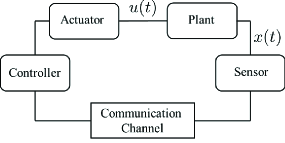
Figure 1: System model.

The plant is described by a scalar, continuous-time, linear time-invariant model as:

$$\dot{x}=Ax(t)+Bu(t)+w(t),$$ (1)

where $x(t)\in\mathbb{R}$ and $u(t)\in\mathbb{R}$ for $t\in[0,\infty)$ are the plant state and control input, respectively, and $w(t)\in\mathbb{R}$ represents the process disturbance. The latter is upper bounded as:

$$|w(t)|\leq M,$$ (2)

where $M$ is a positive real number. In (1), $A$ is a positive real number, $B\in\mathbb{R}$, and

$$|x(0)|\leq L$$ (3)

for some positive real number $L$. We assume that the sensor measures the system state exactly, and the controller acts with infinite precision and without delay. However, the measured state is sent to the controller through a communication channel that only supports a finite data rate and is subject to bounded delay. More precisely, when the sensor transmits packet via the communication channel, the controller will receive the packet entirely and without any error, but with unknown bounded delay.

The sequence of triggering times at which the sensor transmits a packet of length $g(t_{s}^{k})$ bits, is denoted by $\{t_{s}^{k}\}_{k\in\mathbb{N}}$ and the sequence of times at which the controller receives the corresponding packet and decodes it, is denoted by $\{t_{c}^{k}\}_{k\in\mathbb{N}}$. Communication delays are uniformly upper-bounded by $\gamma$, a finite non-negative real number, as follows:

$$\Delta_{k}=t_{c}^{k}-t_{s}^{k}\leq\gamma,$$ (4)

where $\Delta_{k}$ is the $k^{th}$ communication delay. For all $k\geq 1$, we also define the $k^{th}$ triggering interval as

$$\Delta^{\prime}_{k}=t_{s}^{k+1}-t_{s}^{k}.$$ (5)

When referring to a generic triggering or reception time, for convenience we skip the super-script $k$ in $t_{r}^{k}$ and $t_{c}^{k}$.

In this setting, the classical data-rate theorem states that the controller can stabilize the plant if it receives information at least with rate $A/\ln 2$ [31]. Let $b_{s}(t)$ be the number of bits transmitted by the sensor up to time $t$. We define the information transmission rate as

$$R_{s}=\limsup_{t\rightarrow\infty}\frac{b_{s}(t)}{t}.$$

Since at every triggering interval the sensor sends $g(t_{s})$ bits, we have

$$R_{s}=\limsup_{N\rightarrow\infty}\frac{\sum_{k=1}^{N}g(t_{s}^{k})}{\sum_{k=1}^{N}\Delta^{\prime}_{k}}.$$ (6)

At the controller, the estimated state is represented by $\hat{x}$ and evolves during the inter-reception times as

$$\dot{\hat{x}}(t)=A\hat{x}(t)+Bu(t),\quad t\in[t_{c}^{k},t_{c}^{k+1}],$$ (7)

starting from $\hat{x}(t_{c}^{k+})$ with $\hat{x}(0)=\hat{x}_{0}$.

We assume that the sensor has knowledge of the time the actuator performs the control action. This is to ensure that the sensor can also compute $\hat{x}(t)$ for all time $t$. In practice, this corresponds to assuming an instantaneous acknowledgment from the actuator to the sensor via the control input, as discussed in [8, 33]. To obtain such causal knowledge, one can monitor the output of the actuator provided that the control input changes at each reception time. In case the sensor has only access to the system state, one can use a narrowband signal in the control input to excite a specific frequency of the state, that can signal the time at which the control action has been applied. The state estimation error is defined as

$$z(t)=x(t)-\hat{x}(t),$$ (8)

where $z(0)=x(0)-\hat{x}_{0}$. We use this error to determine when a triggering event occurs in our controller design to ensure a property similar to practical stability [34] for the system in (1).

III Control Design

This section proposes our event-triggered control strategy, along with a quantization policy to generate and send packets at every triggering event, to stabilize the scalar, continuous-time linear time-invariant system described in Section II. Along the way, we also characterize a sufficient information transmission rate to accomplish this.

Assume a triggering event occurs when

$$|z(t)|=J,$$ (9)

where $J$ is a positive real number. If the controller knows the triggering time $t_{s}$, then it also knows that $x(t_{s})=\pm J+\hat{x}(t_{s})$. It follows that, it may compute the exact value of $x(t_{s})$ by just transmitting one single bit at every triggering time. In general, however, the controller does not have knowledge of $t_{s}$ because of the delay, but only knows the bound in (4).

Let $\bar{z}(t_{c})$ be an estimate of ${z}(t_{c})$ constructed by the controller knowing that $|z(t_{s})|=v(t_{s})$ and using (4) and the decoded packet received through the communication channel. We define the following updating procedure, called jump strategy

$$\hat{x}(t_{c}^{+})=\bar{z}(t_{c})+\hat{x}(t_{c}).$$ (10)

At triggering time $t_{s}$ the sensor encodes the system state in packet $p(t_{s})$ of size $g(t_{s})$, consisting of the sign of $z(t_{s})$ and a quantized version of $t_{s}$, which we denote by $q(t_{s})$, and send it to the controller. Using the bound in (4) and by decoding the received packet, the controller reconstructs the quantized version of $t_{s}$. Finally, the controller can estimate $z(t_{c})$ as follows:

$$\bar{z}(t_{c})=\text{sign}(z(t_{s}))Je^{A(t_{c}-q(t_{s}))}.$$ (11)

Noting that with the jump strategy (10), we have

$$z(t_{c}^{+})=x(t_{c})-\hat{x}(t_{c}^{+})=z(t_{c})-\bar{z}(t_{c}),$$

the sensor chooses the packet size $g(t_{s})$ large enough to satisfy the following equation for all possible $t_{c}\in[t_{s},t_{s}+\gamma]$

$$|z(t_{c}^{+})|=|z(t_{c})-\bar{z}(t_{c})|\leq\rho_{0}J,$$ (12)

where $0<\rho_{0}<1$ is a constant design parameter. To find a lower bound on the size of the packet so that (12) is ensured, the next result bounds how large the difference $|t_{s}-q(t_{s})|$ of the triggering time and its quantized version can be.

Lemma 1

For the plant-sensor-channel-controller model with plant dynamics (1), estimator dynamics (7), triggering strategy (9), and jump strategy (10), using (11) with $J>\frac{M}{A\rho_{0}}(e^{A\gamma}-1)$, if

$$|t_{s}-q(t_{s})|\leq\frac{1}{A}\ln(1+\frac{\rho_{0}-\frac{M}{JA}(e^{A\gamma}-1)}{e^{A\gamma}})$$ (13)

then (12) holds.

We next propose our quantization algorithm and rely on Lemma 1 to lower bound the packet size to ensure (12).

Theorem 1

Consider the plant-sensor-channel-controller model with plant dynamics (1), estimator dynamics (7), triggering strategy (9), and jump strategy (10). If the control has enough information about $x(0)$ such that state estimation error satisfies $|z(0)|<J$ , there exists a quantization policy that achieves (12) for all $k\in\mathbb{N}$ with a packet size

$$g(t_{s}^{k})\geq\max\left\{0,1+\log\frac{Ab\gamma}{\ln(1+\frac{\rho_{0}-(M/JA)(e^{A\gamma}-1)}{e^{A\gamma}})}\right\},$$ (14)

where $b>1$ and $J>\frac{M}{A\rho_{0}}(e^{A\gamma}-1)$.

Next, we show that using our encoding and decoding scheme, if the sensor has a causal knowledge of the delay in the communication channel, it can compute the state estimated by the controller.

Proposition 1

Consider the plant-sensor-channel-controller model with plant dynamics (1), estimator dynamics (7), triggering strategy (9), and jump strategy (10). Using (11) and the quantization policy described in Theorem 1, if the sensor has causal knowledge of delay in the communication channel, then the sensor can calculate $\hat{x}(t)$ at each time $t$.

Next, we show that the proposed event-triggered scheme has triggering intervals that are uniformly lower bounded and consequently does not show “Zeno behavior”, namely infinitely many triggering events in a finite time interval

Lemma 2

Consider the plant-sensor-channel-controller model with plant dynamics (1), estimator dynamics (7), triggering strategy (9), and jump strategy (10). If the packet size satisfies (14) for all $k\in\mathbb{N}$, and $J>\frac{M}{A\rho_{0}}(e^{A\gamma}-1)$ then for all $k\in\mathbb{N}$

$$t_{s}^{k+1}-t_{s}^{k}\geq\frac{1}{A}\ln(\frac{J+\frac{M}{A}}{\rho_{0}J+\frac{M}{A}}).$$ (15)

The frequency with which transmission events are triggered is captured by the triggering rate

$$R_{tr} =\limsup_{N\rightarrow\infty}\frac{N}{\sum_{k=1}^{N}\Delta^{\prime}_{k}}.$$ (16)

Using Lemma 2, we deduce that

$$R_{tr}\leq\frac{A}{\ln(\frac{J+\frac{M}{A}}{\rho_{0}J+\frac{M}{A}})}$$

for all initial conditions and possible delay and process noise values. Combining this bound and Theorem 1, we arrive at the following result.

Corollary 1

Consider the plant-sensor-channel-controller model with plant dynamics (1), estimator dynamics (7), triggering strategy (9), and jump strategy (10). If the control has enough information about $x(0)$ such that state estimation error satisfies $|z(0)|<J$ with $J>\frac{M}{A\rho_{0}}(e^{A\gamma}-1)$, there exists a quantization policy that achieves (12) for all $k\in\mathbb{N}$ and for all delay and process noise realization with an information transmission rate

$$R_{s}\geq$$ (17)

$$\frac{A}{\ln(\frac{J+\frac{M}{A}}{\rho_{0}J+\frac{M}{A}})}\max\left\{0,1+\log\frac{Ab\gamma}{\ln(1+\frac{\rho_{0}-(M/JA)(e^{A\gamma}-1)}{e^{A\gamma}})}\right\}.$$

Figure 2 shows the sufficient transmission rate as a function of the bound $\gamma$ on the channel delay. As expected, the rate starts from zero and as $\gamma$ increases, goes above the data-rate theorem.

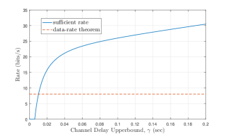
Figure 2: Illustration of sufficient transmission rate as a function of $\gamma$. Here, A=5.5651, $\rho_{0}=0.1$, $b=1.0001$, $M=0.2$, and $J=\frac{M}{A\rho_{0}}(e^{A\gamma}-1)+0.1$.

The next result ensures a property similar to practical stability [34] for the system in (1).

Theorem 2

Consider the plant-sensor-channel-controller model with plant dynamics (1), estimator dynamics (7), triggering strategy (9), and jump strategy (10). Assume the pair $(A,B)$ is stabilizable. If the control has enough information about $x(0)$ such that state estimation error satisfies $|z(0)|<J$ with $J>\frac{M}{A\rho_{0}}(e^{A\gamma}-1)$, and if the sensor use the quantization policy proposed in Theorem 1, then there exists a time $T_{0}$ and a real number $\kappa$ such that, $|x(t)|\leq\kappa$ for all $t\geq T_{0}$, provided that the packet size is lower bounded by (14).

From Corollary 1, it follows that a transmission rate lower bounded by (17) is sufficient to ensure the property similar to practical stability stated in Theorem 2.

IV Simulation

We now implement the proposed event-triggered control scheme on a dynamical system such as a linearized inverted pendulum. In this section, initially, a mathematical model of an inverted pendulum mounted on a cart is presented. Then the nonlinear equations are linearized about the equilibrium state of the system. In addition, a canonical transformation is applied to the linear time-invariant system to decouple the equations of motion.

We consider the two-dimensional problem where motion of the pendulum is constrained in a plane and its position can be measured by angle $\theta$. We assume that inverted pendulum has mass $m_{1}$, length $l$, and moment of inertia $I$. Also, the pendulum is mounted on top of a cart of mass $m_{2}$ constrained to move in $y$ direction. Nonlinear equations governing the motion of the cart and pendulum can be written as follows:

$$(m_{1}+m_{2})\ddot{y}+\nu\dot{y}+m_{1}l\ddot{\theta}\cos\theta-m_{1}l\dot{\theta}^{2}sin\theta=F$$

$$(I+m_{1}l^{2})\ddot{\theta}+m_{1}g_{0}lsin\theta=-m_{1}l\ddot{y}cos\theta$$

where $\nu$ is the damping coefficient between the pendulum and the cart and $g_{0}$ is the gravitational acceleration.

IV-A Linearizion

We define $\theta=\pi$ as the equilibrium position of the pendulum and $\phi$ as small deviations from $\theta$. We derive the linearized equations of motion using small angle approximation. Let’s define state variable $s=[y,\dot{y},\phi,\dot{\phi}]^{T}$, where $y$ and $\dot{y}$ are the position and velocity of the cart respectively. Assuming $m_{1}=0.2$ kg, $m_{2}=0.5$ kg, $\nu=0.1$ N/m/s, $l=0.3$ m, $I=0.006$ kg/m², one can write the evolution of $s$ in time as follows:

$$\dot{s}=As(t)+Bu(t)+w(t),$$ (18)

$$A=\begin{bmatrix}0&1&0&0\\ 0&-0.1818&2.6730&0\\ 0&0&0&1\\ 0&-0.4545&31.1800&0\end{bmatrix},B=\begin{bmatrix}0\\ 1.8180\\ 0\\ 4.5450\end{bmatrix}.$$

In addition, we add the process noise $w(t)$ to the linearized system model. $w(t)$ is a vector of length four, and we assume that all the elements of $w(t)$ are upper bounded $M$. Also, a simple feedback control law can be derived for  (18) as $u=-ks$ where $k$ is chosen such that $A-Bk$ is Hurwitz. We let $k$ be as follows $k=\begin{bmatrix}-1.00&-2.04&20.36&3.93\end{bmatrix}$.

Note that although Theorem 1 holds for the linear system with any worst-case delay, the linearizion is only valid for sufficiently small values of $\gamma$.

IV-B Diagonalization

The eigenvalues of the open-loop gain of the system $A$ are $e=\begin{bmatrix}0&-5.6041&-0.1428&5.5651\end{bmatrix}$. Hence, three of the four modes of the system are stable and do not need any actuation. Also, the open-loop gain of the system $A$ is diagonalizable (All eigenvalues of $A$ are distinct). As a result, diagonalization of the matrix $A$, enables us to apply Theorem 1 to the unstable mode of the system, and consequently stabilize the whole system.

Using the eigenvector matrix $P$, we diagonalize the system to obtain

$$\dot{\tilde{s}}=\tilde{A}\tilde{s}(t)+\tilde{B}\tilde{u}(t)+\tilde{w}(t)$$ (19)

where

$$\tilde{A}=\begin{bmatrix}0&0&0&0\\ 0&-5.6041&0&0\\ 0&0&-0.1428&0\\ 0&0&0&5.5651\end{bmatrix},\tilde{B}=\begin{bmatrix}10.0000\\ -2.3865\\ 10.0979\\ 2.2513\end{bmatrix}$$

$\tilde{s}(t)=P^{-1}s(t)$ and $\tilde{w}(t)=P^{-1}w(t)$. Moreover, $\tilde{u}(t)=-\tilde{k}\tilde{s}(t)$ where $\tilde{k}=kP$, that is, $\tilde{k}=\begin{bmatrix}-1.0000&-0.1295&0.7422&7.2624\end{bmatrix}$.

IV-C Event-triggered design

For the first three coordinates of the diagonalized system (19) which are stable the state estimation $\hat{s}$ at the controller simply constructs as follows:

$$\dot{\hat{s}}=\tilde{A}\hat{s}(t)+\tilde{B}\tilde{u}(t)$$

starting from $\hat{s}(0)$. The unstable mode of the system is as follow

$$\dot{\tilde{s}}_{4}=5.5651\tilde{s}_{4}(t)+2.2513\tilde{u}(t)+\tilde{w}_{4}(t)$$ (20)

Then using the problem formulation in section II the estimated state for the unstable mode $\hat{s}_{4}$ evolves during the inter-reception times as

$$\dot{\hat{s}}_{4}(t)=5.5651\hat{s}_{4}(t)+2.2513\tilde{u}(t),\quad t\in[t_{c}^{k},t_{c}^{k+1}],$$ (21)

starting from $\hat{s}_{4}(t_{c}^{k+})$ and $\hat{s}_{4}(0)$.

The triggering occurs when

$$|\tilde{z}_{4}(t)|=|\tilde{s}_{4}(t)-\hat{s}_{4}(t)|=J,$$

where $|\tilde{z}_{4}(t)|$ is the estate estimation error for the unstable mode. Let $\lambda_{4}$ be the eigenvalue corresponding to the unstable mode which is equal to $5.5651$. Then using Theorem 1 we choose

$$J=\frac{M}{\lambda_{4}\rho_{0}}(e^{\lambda_{4}\gamma}-1)+0.005,$$

and the size of the packet for all $t_{s}$ to be

$$g(t_{s})=\max\left\{1,\lceil 1+\log\frac{Ab\gamma}{\ln(1+\frac{\rho_{0}-(M/JA)(e^{A\gamma}-1)}{e^{A\gamma}})}\rceil\right\},$$

where $b=1.0001$, $\rho_{0}=0.9$.

The packet size for the simulation has two differences from the lower bound provided in Theorem 1. Because the packet size should be an integer we used the ceiling operator, and since we should have at least one bit, to send a packet we take the maximum between 1 and the result of the ceiling operator.

IV-D Simulation Results

The following simulation parameters are chosen for the system: simulation time $T=5$ seconds, sampling time $\Delta t=0.005$ seconds, $\tilde{s}(0)={P^{-1}}[0,0,0,0.1001]^{T}$, and $\hat{s}(0)={P^{-1}}[0,0,0,0.10]^{T}$.

Theorem 1 is developed based on a continuous system but the simulation environments are all digital. We tried to make the discrete model as close to the continuous model by choosing a very small sampling time. However, the minimum upper bound for the channel delay will be equal to one sampling time. A set of three simulations are carried out as follows. For simulation (a) we assumed the process disturbance is zero and channel delay upper bounded by sampling time. In simulation (b) we assumed that the process disturbance upper bounded by $M$ and channel delay upper bounded by sampling time. Finally, for simulation (c) we assumed that the process disturbance upper bounded by $M$ and channel delay upper bounded by $\gamma$.

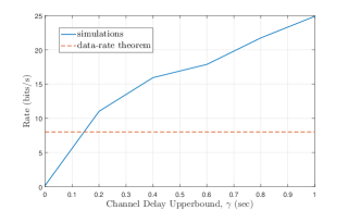
Figure 3: Information transmission rate in simulations compared to the data-rate theorem. Note that the rate calculated from simulations does not start at zero worst-case delay because the minimum channel delay upper bound is equal to one sampling time (0.005 seconds in this example). $M$ is chosen to be 0.2 in these simulations, and simulation time is $T=5$ seconds.

Simulation results for simulation (a), (b) and (c) are presented in Figure 4. Each column represents a different simulation. The first row shows the triggering function for $\tilde{s}_{4}$ (20) and the absolute value of state estimation error for the unstable coordinate, that is, $|\tilde{z}_{4}(t)|=|\tilde{s}_{4}(t)-\hat{s}_{4}(t)|$. As soon as the absolute value of this error is equal or greater than the triggering function, sensor transmit a packet, and the jumping strategy adjusts $\hat{s}_{4}$ at the reception time to practically stabilize the system. The amount this error exceeds the triggering function depends on the random channel delay with upper bound $\gamma$. In the second row of Figure 4, the evolution of the unstable state (20) and its state estimation are presented (21). Finally, the last row in Figure 4 represents the evolution of all actual states of the linearized system (18) in time.

Finally, Figure 3 presents the simulation of information transmission rate versus the worst-case delay in communication channel $\gamma$ for stabilizing the linearized model of the inverted pendulum.

$M=0.0$, $\gamma=0.005$ sec, $g(t_{s})=1$ bit	$M=0.05$, $\gamma=0.005$ sec, $g(t_{s})=1$ bit	$M=0.05$, $\gamma=0.1$ sec, $g(t_{s})=4$ bits
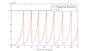
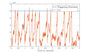
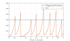
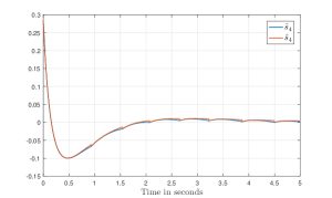
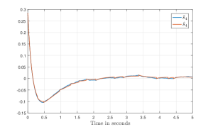
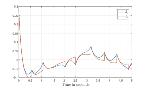
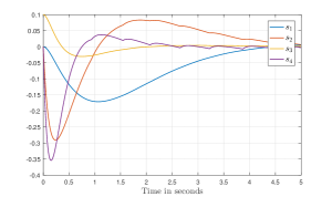
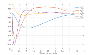
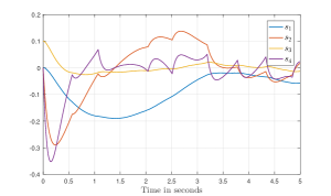
(a)	(b)	(c)

Figure 4: Simulation results: The first row represents the absolute value of state estimation error for the unstable mode of the system (20). The second row represents the unstable mode (20), and its state estimate (21). Finally, and the last row represents the evolution of all actual states of the real system (18) in time.

V Conclusions

We have presented an event-triggered control scheme for the stabilization of noisy, scalar, continuous, linear time-invariant systems over a communication channel subject to random bounded delay. We have also developed an algorithm for coding/decoding the quantized version of the estimated states, leading to the characterization of a sufficient transmission rate for stabilizing the system. We have illustrated our results on a linearization of the inverted pendulum for different channel delay bounds. Future work will study the identification of necessary conditions on the transmission rate, the investigation of the effect of delay on nonlinear systems, and the implementation of the proposed control strategies on real systems.

References

- [1] J. P. Hespanha, P. Naghshtabrizi, and Y. Xu, “A survey of recent results in networked control systems,” Proceedings of the IEEE, vol. 95, no. 1, pp. 138–162, 2007.
- [2] K.-D. Kim and P. R. Kumar, “Cyber–physical systems: A perspective at the centennial,” Proceedings of the IEEE, vol. 100 (Special Centennial Issue), pp. 1287–1308, 2012.
- [3] R. M. Murray, K. J. Astrom, S. P. Boyd, R. W. Brockett, and G. Stein, “Future directions in control in an information-rich world,” IEEE Control Systems, vol. 23, no. 2, pp. 20–33, 2003.
- [4] W. S. Wong and R. W. Brockett, “Systems with finite communication bandwidth constraints. II. stabilization with limited information feedback,” IEEE Transactions on Automatic Control, vol. 44, no. 5, pp. 1049–1053, 1999.
- [5] J. Baillieul, “Feedback designs for controlling device arrays with communication channel bandwidth constraints,” in ARO Workshop on Smart Structures, Pennsylvania State Univ, 1999, pp. 16–18.
- [6] S. Tatikonda and S. Mitter, “Control under communication constraints,” IEEE Transactions on Automatic Control, vol. 49, no. 7, pp. 1056–1068, 2004.
- [7] G. N. Nair and R. J. Evans, “Stabilizability of stochastic linear systems with finite feedback data rates,” SIAM Journal on Control and Optimization, vol. 43, no. 2, pp. 413–436, 2004.
- [8] A. Sahai and S. Mitter, “The necessity and sufficiency of anytime capacity for stabilization of a linear system over a noisy communication link. Part I: Scalar systems,” IEEE Transactions on Information Theory, vol. 52, no. 8, pp. 3369–3395, 2006.
- [9] S. Tatikonda and S. Mitter, “Control over noisy channels,” IEEE transactions on Automatic Control, vol. 49, no. 7, pp. 1196–1201, 2004.
- [10] A. S. Matveev and A. V. Savkin, Estimation and control over communication networks. Springer Science & Business Media, 2009.
- [11] A. Khina, W. Halbawi, and B. Hassibi, “(almost) practical tree codes,” in 2016 IEEE International Symposium on Information Theory (ISIT), July 2016, pp. 2404–2408.
- [12] R. T. Sukhavasi and B. Hassibi, “Linear time-invariant anytime codes for control over noisy channels,” IEEE Transactions on Automatic Control, vol. 61, no. 12, pp. 3826–3841, 2016.
- [13] P. Minero, M. Franceschetti, S. Dey, and G. N. Nair, “Data rate theorem for stabilization over time-varying feedback channels,” IEEE Transactions on Automatic Control, vol. 54, no. 2, p. 243, 2009.
- [14] P. Minero, L. Coviello, and M. Franceschetti, “Stabilization over Markov feedback channels: the general case,” IEEE Transactions on Automatic Control, vol. 58, no. 2, pp. 349–362, 2013.
- [15] V. Kostina, Y. Peres, M. Z. Rácz, and G. Ranade, “Rate-limited control of systems with uncertain gain,” 54th Annual Allerton Conference on Communication, Control, and Computing, pp. 1189–1196, 2016.
- [16] G. Yang and D. Liberzon, “Feedback stabilization of switched linear systems with unknown disturbances under data-rate constraints,” IEEE Transactions on Automatic Control, 2017.
- [17] G. Ranade and A. Sahai, “Control capacity,” in Information Theory (ISIT), 2015 IEEE International Symposium on. IEEE, 2015, pp. 2221–2225.
- [18] J. Ding, Y. Peres, G. Ranade, and A. Zhai, “When multiplicative noise stymies control,” arXiv preprint arXiv:1612.03239, 2016.
- [19] G. Ranade and A. Sahai, “Non-coherence in estimation and control,” in Communication, Control, and Computing (Allerton), 2013 51st Annual Allerton Conference on. IEEE, 2013, pp. 189–196.
- [20] S. Tatikonda, A. Sahai, and S. Mitter, “Stochastic linear control over a communication channel,” IEEE transactions on Automatic Control, vol. 49, no. 9, pp. 1549–1561, 2004.
- [21] V. Kostina and B. Hassibi, “Rate-cost tradeoffs in control,” in Communication, Control, and Computing (Allerton), 2016 54th Annual Allerton Conference on. IEEE, 2016, pp. 1157–1164.
- [22] A. Khina, Y. Nakahira, Y. Su, and B. Hassibi, “Algorithms for optimal control with fixed-rate feedback,” in 2017 IEEE 56th Annual Conference on Decision and Control (CDC), Dec 2017, pp. 6015–6020.
- [23] A. Khina, G. M. Pettersson, V. Kostina, and B. Hassibi, “Multi-rate control over awgn channels via analog joint source-channel coding,” in Decision and Control (CDC), 2016 IEEE 55th Conference on. IEEE, 2016, pp. 5968–5973.
- [24] M. J. Khojasteh, P. Tallapragada, J. Cortés, and M. Franceschetti, “The value of timing information in event-triggered control: The scalar case,” 54th Annual Allerton Conference on Communication, Control, and Computing, pp. 1165–1172, Sep. 2016.
- [25] P. Tallapragada and J. Cortés, “Event-triggered stabilization of linear systems under bounded bit rates,” IEEE Transactions on Automatic Control, vol. 61, no. 6, pp. 1575–1589, 2016.
- [26] L. Li, X. Wang, and M. Lemmon, “Stabilizing bit-rates in quantized event triggered control systems,” in Proceedings of the 15th ACM international conference on Hybrid Systems: Computation and Control. ACM, 2012, pp. 245–254.
- [27] J. Pearson, J. P. Hespanha, and D. Liberzon, “Control with minimal cost-per-symbol encoding and quasi-optimality of event-based encoders,” IEEE Transactions on Automatic Control, vol. 62, no. 5, pp. 2286–2301, 2017.
- [28] Q. Ling, “Bit rate conditions to stabilize a continuous-time scalar linear system based on event triggering,” IEEE Transactions on Automatic Control, 2017, to appear.
- [29] S. Linsenmayer, R. Blind, and F. Allgöwer, “Delay-dependent data rate bounds for containability of scalar systems,” IFAC-PapersOnLine, vol. 50, no. 1, pp. 7875–7880, 2017.
- [30] E. Kofman and J. H. Braslavsky, “Level crossing sampling in feedback stabilization under data-rate constraints,” in 45st IEEE Conference on Decision and Control (CDC). IEEE, 2006, pp. 4423–4428.
- [31] M. J. Khojasteh, P. Tallapragada, J. Cortés, and M. Franceschetti, “The value of timing information in event-triggered control,” arXiv preprint arXiv:1609.09594, 2016.
- [32] M. J. Khojasteh, P. Tallapragada, J. Cortés, and M. Franceschetti, “Time-triggering versus event-triggering control over communication channels,” in 2017 IEEE 56th Annual Conference on Decision and Control (CDC), Dec 2017, pp. 5432–5437.
- [33] Q. Ling, “Bit rate conditions to stabilize a continuous-time linear system with feedback dropouts,” IEEE Transactions on Automatic Control, vol. PP, no. 99, pp. 1–1, 2017.
- [34] V. Lakshmikantham, S. Leela, and A. A. Martynyuk, Practical stability of nonlinear systems. World Scientific, 1990.