Models for the Unusual Supernova iPTF14hls

Abstract

Supernova iPTF14hls maintained a bright, variable luminosity for more than 600 days, while lines of hydrogen and iron in its spectrum had different speeds, but showed little evolution. Here several varieties of models are explored for iPTF14hls-like events. They are based upon circumstellar medium (CSM) interaction in an ordinary supernova, pulsational pair-instability supernovae (PPISN), and magnetar formation. Each is able to explain the enduring emission and brightness of iPTF14hls, but has shortcomings when confronted with other observed characteristics. The PPISN model can, in some cases, produce a presupernova transient like the one observed at the site of iPTF14hls in 1954. It also offers a clear path to providing the necessary half solar mass of material at $\sim 5\times 10^{16}$ cm for CSM interaction to work, and can give an irregular light curve without invoking additional assumptions. It explains the 4000 km s^-1 seen in the iron lines, but without additional energy input, strains to provide enough matter to explain the nearly constant 8000 km s^-1 velocity seen in H_α. Magnetar models can also explain many of the observed features, but give a smooth light curve and may require an evolving magnetic field strength. Their dynamics may be difficult to reconcile with the observation of slow-moving hydrogen at late times. The various models predict different spectral characteristics and a remnant that, today, could be a black hole, magnetar, or even a star. Further observations and calculations of radiation transport will narrow the range of possibilities.

1. INTRODUCTION

iPTF14hls was discovered by the iPTF survey in September, 2014 (Arcavi et al., 2017). Though initially sparsely sampled, the failure of the supernova to decline marked it for more intensive investigation. In January, 2015 it was determined to be a Type II supernova. For the next year, the supernova displayed an irregular light curve with multiple episodes of brightening during which the luminosity varied by about 50%. The total energy emitted in light during the first 600 days was about $2.2\times 10^{50}$ erg, making iPTF14hls a luminous, but not particularly “superluminous” supernova. There is also some evidence of a supernova-like transient having happened at the same site in 1954. The long duration of iPTF14hls precludes the supernova from being a purely recombination event like most Type IIp supernovae. The required mass and energy are too large. Nor is a radioactive energy source the explanation. No radioactivity with the appropriate half life is produced with sufficient abundance in any model.

One is thus left with two possibilities: 1) iPTF14hls was collisionally powered, its light coming from shells of matter that collided over a long period of time, possibly augmented by a central source; or 2) the event was an extreme example, in terms of duration and spectrum, of magnetar-illuminated supernovae. Both possibilities were suggested by Arcavi et al. (2017), with the underlying cause for the shell ejections in case 1 attributed to a pulsational-pair instability supernova (e.g. Woosley et al., 2007; Woosley, 2017a).

Here, both possibilities are explored. First, the outcome of an ordinary supernova interacting with a dense wind is considered (§ 2). Given a free choice of wind parameters, one can easily find an approximate fit to the global light curve and the high velocity (hydrogenic) component of the spectrum, though the origin of the lower velocity iron lines is less clear in a one-dimensional model (though see Andrews & Smith, 2017, and § 3.3). Even more problematic, the reason why a star would lose roughly a solar mass of high velocity material during the last few decades of its life is not obvious unless the star dies as a PPISN.

§ 3 thus considers PPISN explanations for iPTF14hls. The models are of three sorts: 1) those that might be capable of producing both the 1954 and 2014 transients, but which leave a stellar core that has not yet collapsed (§ 3.1); 2) slightly lighter stars where the pulsing activity is restricted to the last decade of the star’s life, and which experience iron-core collapse while the light curve is still in progress (§ 3.2); and 3) hybrid models that invoke an asymmetric explosion with one component due to the collapse of the iron core to a compact object (§ 3.3). Each has strengths and weaknesses. All are able to explain the approximate duration and brightness of the light curve and, since each can occur in nature, may ultimately appear as iPTF14hls-like supernovae, if not as iPTF14hls itself. Each PPISN model has difficulty, though, explaining the high velocity (8000 km s^-1) H_α component of iPTF14hls.

Magnetar models are considered in § 4. It is not difficult to find a two parameter fit that approximately tracks the overall bolometric light curve. The very bright initial display of the magnetar is masked by the overlying star and adiabatically degraded alleviating a concern voiced by Arcavi et al. (2017). For the 20 $M_{\odot}$ supernova model considered, most of the pulsar energy is invisible for the first 100 days. Models with greater explosion energies and more mass loss give higher speeds that may be necessary to explain the spectrum. If the same neutron star is responsible for accelerating the helium core to 4000 km s^-1 and making the light curve, magnetic field decay must be invoked. While magnetar models are potentially successful at explaining many characteristics of iPTF14hls, they would not give the spectroscopic features characteristic of CSM interaction that have been recently reported by (Andrews & Smith, 2017) and would not, in any obvious way, produce a transient in 1954.

§ 5 summarizes the strengths and weaknesses of the various models and makes some suggestions for future observations.

Where stellar and supernova models are employed, they have all been calculated using the KEPLER code (Weaver, Zimmerman, & Woosley, 1978; Woosley et al., 2002) using physics described in Sukhbold et al. (2016), Woosley (2017a), and Sukhbold et al. (2018).

2. Circumstellar Interaction

Circumstellar medium (CSM) interaction is interesting both as a generic model for iPTF14hls, and as a way to set some useful fiducial characteristics for later use. iPTF14hls emitted at least $2.2\times 10^{50}$ erg of light over a period of approximately 600 days (Arcavi et al., 2017) (additional light may not have been optical), implying an average, though variable, luminosity $\sim 5\times 10^{42}$ erg s^-1. In the CSM interaction model, this light is emitted as the outer layers of a supernova plow into a lower density medium at a radius where conversion of kinetic energy to optical radiation was efficient, i.e., $\sim 10^{15}$ - 10¹⁶ cm. An independent estimate of the radius of the CSM comes from the $\sim 600$ day duration of the event times the highest velocity maintained throughout the event in the spectrum, $\sim 8000$ km s^-1 for H_α, or $\lower 0.43057pt\hbox{\hbox to0.0pt{\raise 2.58334pt\hbox{\hskip 1.29167pt{{$\scriptscriptstyle>$}}}\hss} \kern-1.72218pt{{$\scriptscriptstyle\sim$}}}5\times 10^{16}$ cm. In order that the velocity in the spectrum not significantly slow during the observations, there must be at least several times more mass in the interacting ejecta than in the CSM. The kinetic energy in the ejecta must also be at least several times what was seen in radiation or no kinetic energy would be left over after 600 days. A kinetic energy $E\lower 0.43057pt\hbox{\hbox to0.0pt{\raise 2.58334pt\hbox{\hskip 1.29167pt{{$\scriptscriptstyle>$}}}\hss} \kern-1.72218pt{{$\scriptscriptstyle\sim$}}}5\times 10^{50}$ erg is implied. Observed speeds throughout iPTF14hls were 4000 (for iron) to 8000 km s^-1 (for hydrogen), so the kinetic energy implies a mass for the impacting ejecta of at least one to several solar masses. The presupernova may have ejected a much larger mass that moved more slowly. These are the characteristics of just the “working surface” of the shock, and are minima for the total ejected mass and energy. The mass of the swept up CSM would be comparable, but less to avoid excessive deceleration.

For a solar mass to exist at $5\times 10^{16}$ cm implies either explosive mass loss or a steady loss rate  $\scriptscriptstyle>$ $\scriptscriptstyle\sim$0.01$v_{7}$ $M_{\odot}$ y^-1 where $v_{7}$ is the wind speed in units of 100 km s^-1. This mass loss rate must persist for 100/$v_{7}$ years. Again the actual mass loss could be bigger because only the inner, slowest moving matter will interact and produce the high luminosity. Ejecting one solar mass at 1000 km s^-1 requires 10⁴⁹ erg.

2.1. Approximations and Models

Some approximate scaling relations will be useful. Consider the simplest case of an ejected shell with mass, $M_{\rm eject}$, and energy, $E$, that encounters a previously ejected shell with mass, $M_{\rm CSM}$, outer radius, $R$, and negligible inner radius. Chevalier (1982a) has studied the general case in which both the CSM and homologously coasting supernova ejecta have initial densities that depend on a power law of the radius, $\rho_{\rm CSM}\propto r^{-s}$ and $\rho_{\rm ejecta}\propto r^{-n}$ respectively, and gives useful scaling relations for the radii and masses of the shocked CSM and ejecta as a function of time. Chevalier (1982ab) considered the special case $s=2$, which corresponds to a stellar wind with constant speed and mass loss rate. For simplicity, that simple case will be adopted here, though the real situation may be different, especially when the mass loss is explosive.

Then the unknowns are $M_{\rm eject}$, $E$, $n$, $M_{\rm CSM}$, and $R$. Actually it is the ratio $M_{\rm CSM}/R$ that matters, and not the individual terms, so long as the radius of the shock remains bounded by $R$. This is because for the special case $s$ = 2, $\rho r^{2}$ = constant = $q=M_{\rm CSM}/(4\pi R)$. As Chevalier notes, and as will later be confirmed here, the interaction region is thin, so one can, to good approximation, assign a single radius, $r(t)$, to the forward and reverse shocks (Chevalier, 1982b),

$$r(t)\ =\ \left[\frac{2U^{n}}{(n-4)(n-3)\,q)}\right]^{1/(n-2)}\,t^{(n-3)/(n-2)}.{}$$ (1)

Here $U$ is a constant used to normalize the density distribution in the supernova ejecta, so that at time, $t$, and radius, $r$, $\rho_{\rm ejecta}(r,t)=t^{-3}(r/(tU))^{-n}$. For the special case $n=7$, Chevalier (1982c) gives

$$r^{(7)}\ =\ 0.823\,\left(\frac{E^{2}}{M_{\rm eject}q}\right)^{2/5}\,t^{4/5},{}$$ (2)

where the superscript 7 refers to the assumption $n=7$. Normalizing to conditions we will find appropriate for iPTF14hls, $E=4\times 10^{50}$ erg, $M_{\rm eject}$ = 1.0 $M_{\odot}$, $M_{\rm CSM}$ = 0.4 $M_{\odot}$, and $R_{\rm CSM}=4.5\times 10^{16}$,

$$r^{(7)}\ =\ 1.4\times 10^{16}\ t_{7}^{4/5}\ {\rm cm},{}$$ (3)

where $t_{7}$ is time in units of $10^{7}$ s.

As Chevalier notes, $n=7$ is appropriate to Type Ia supernovae and $n=12$ may be a better choice for Type II supernovae occurring in red supergiants. Then one must make a choice for $U$ in eq. 1. Based upon observations of Type II supernovae, Chevalier (1982b) suggests $U$ is a few times $10^{9}$. This is consistent with the models of Woosley & Heger (2007). Here $U=2.5\times 10^{9}$ is adopted, giving

$$r^{(12)}\ =\ 8.5\times 10^{15}\,t_{7}^{9/10}\ {\rm cm}.{}$$ (4)

In fact, use of $n=12$ is inexact for a Type II supernova, especially as one goes deeper into the ejecta as is appropriate for the present problem. The CSM is also unlikely to have the ideal s = 2 distribution of a wind at constant speed and mass loss rate, so either formula would suffice. Here we will use $r^{(12)}$.

Continuing to assume a thin shell with only a single radius and speed, the shock velocity is the derivative of the radius,

$$v_{s}^{(12)}\ =\ 7700\,t_{7}^{-1/10}\ {\rm km\ s^{-1}}.{}$$ (5)

The bolometric luminosity is given by

$$L\ =\ 2\pi r^{2}\rho_{\rm CSM}\,v_{s}^{3}\ =\ 2\pi qv_{s}^{3}$$ (6)

$$=\ 0.5M_{\rm CSM}/R_{\rm CSM}\,v_{s}^{3}$$ (7)

$$=\ 4.0\times 10^{42}\,t_{7}^{-3/10}\ {\rm erg\ s^{-1}},{}$$ (8)

where the superscript $n=12$ has been omitted. The very slow evolution of the velocity and luminosity in these equations resemble that seen in iPTF14hls, and is a consequence of the steep power-law dependence of the density in the supernova ejecta. For the $n=7$ case, velocity and luminosity would have declined a bit more steeply as $t^{-1/5}$ and $t^{-3/5}$, respectively. As matter deeper in the ejecta interacts at later times, one expects $n$ to decrease and the rate of decline to increase.

To test these approximations, a 15 $M_{\odot}$ supernova with a total explosion kinetic energy of $2.4\times 10^{51}$ erg (Woosley & Heger, 2007) was surrounded by a low density shell of 0.4 $M_{\odot}$ consisting of hydrogen and helium with an outer radius of $4.5\times 10^{16}$ cm. Within the shell, $\rho r^{2}$ was a constant, implying $q=1.41\times 10^{15}$ g cm^-1. This value for $q$ will prove a useful constraint for successful CSM models throughout the paper. The presupernova star, without the artificial CSM, had a total mass of 12.79 $M_{\odot}$, 8.52 $M_{\odot}$ of which was its low density hydrogenic envelope with radius $5.65\times 10^{13}$ cm. The unconfined 15 $M_{\odot}$ supernova developed $6.6\times 10^{50}$ erg in its outer 1.0 $M_{\odot}$ of ejecta, but, including the CSM, a third of that energy was radiated during the first 600 days, so this is close to the estimate used in developing eq. 3.

The resulting light curve is shown in Fig. 1. The event is particularly bright during the first 100 days when iPTF14hls was not well sampled because the underlying supernova contributes appreciably to the CSM interaction in producing the total luminosity. This contribution would be greatly reduced if the progenitor had been a blue supergiant (BSG). It would also have been slightly reduced or shortened if the hydrogen envelope were less massive or the explosion energy smaller. After 100 days, the light curve agrees well with eq. 8 and with iPTF14hls for the fiducial parameters.

Fig. 2 shows the density and velocity evolution for this model 280 days after core collapse. It is interesting that this long bright supernova can be powered by the interaction of only about 1 $M_{\odot}$ of ejecta with a modest kinetic energy. Also interesting is the pile up of the ejected matter and swept up CSM into a thin, dense shell. Half way into the supernova, 0.67 $M_{\odot}$ has piled up in a thin shell with a density roughly five orders of magnitude greater than the medium into which it is moving. This shell moves with nearly uniform velocity and justifies the assumption of a single radius for the forward and reverse shocks made in the analytic approximation. In a multi-dimensional calculation this shell would be unstable and spread over a region $\delta r/r\lower 0.43057pt\hbox{\hbox to0.0pt{\raise 2.58334pt\hbox{\hskip 1.29167pt{{$\scriptscriptstyle>$}}}\hss} \kern-1.72218pt{{$\scriptscriptstyle\sim$}}}$ 10%, but a large density contrast would still persist (Chen et al., 2014). The KEPLER code cannot accurately calculate the properties of the photosphere for a thin shock wave in matter that has recombined and is interacting in a region optically thin to electron scattering. It is assumed throughout this paper that most of the radiation comes out in the optical waveband. iPTF14hls was not bright in radio or x-rays (Arcavi et al., 2017). The flux is well determined in the model from momentum conservation, but not its temperature. One can speculate, however, that the photosphere lies within this dense fast moving shell. If fully ionized, the shell would be optically thick and the surroundings quite thin. Perhaps that accounts for the broad hydrogen lines in the spectrum (Chevalier & Fransson, 1994). Clearly much work remains to be done on the radiation transport.

While the qualitative agreement with the light curve and speed of the fastest moving hydrogen with what was observed in iPTF14hls are good, there are several deficiencies in this simple model. The light curve lacks the “flares “ seen in the observations, though an inhomogeneous CSM could be invoked. The 4000 km s^-1 spectral features go unexplained in the simple isotropic model, though a two component, anisotropic explosion with slower speeds at some angles might remedy that (Andrews & Smith, 2017). A large increase in the mass of the circumstellar shell ($q$ in eq. 1) would be required though to slow the speed by a factor of two in some directions. The shell mass assumed, 0.4 $M_{\odot}$, was already substantial since the minimum radius is already set by the duration of the event. The desired variation might be more easily achieved by invoking an anisotropic explosion, i.e., changing U.

The possible pre-explosive outburst in 1954 would also require an additional explanation, but perhaps most challenging is the lack of a clear explanation of just such a massive circumstellar shell came to be ejected just before the supernova.

Figure 1.— Bolometric light curve for the explosion of a 15 $M_{\odot}$ supernova when that explosion is surrounded by a low density shell of matter with mass 0.4 $M_{\odot}$ and outer radius $4.5\times 10^{16}$ cm (solid dark line). The explosion energy of the supernova was $2.4\times 10^{51}$ erg, but only the outer solar mass with initial kinetic energy $6.6\times 10^{50}$ erg participated in the circumstellar interaction during the time shown. During the first 100 days, the underlying supernova adds appreciably to the circumstellar interaction in producing light. Also shown as the dashed line is the effect of increasing the speed of the outer layers of the model by 25%. The dot-dashed line shows the approximation discussed in the text for n = 12 (eq. 4). The triple-dot dashed line is for n = 8, (eq. 3), with $M_{\rm eject}=1.0$ $M_{\odot}$, $M_{\rm CSM}=0.4$ $M_{\odot}$, $R_{\rm CSM}=4.5\times 10^{16}$ cm, and $E=4\times 10^{50}$ erg.

Figure 2.— Velocity and density for two times in the outer layers of the 15 $M_{\odot}$ supernova model shown in Fig. 1. At the earlier time shown, 1.6 days after core collapse, the surface layers of the supernova are first encountering the circumstellar medium. The later time, 280 days post collapse, is about half way through the light curve. 0.67 $M_{\odot}$ has piled up in a thin dense shell currently at a radius of $1.84\times 10^{16}$ cm moving at 6850 km s^-1. This shell would be unstable to break up in 2 or 3 dimensions.

2.2. Constraints on Gravity Wave-Driven Mass Loss

How did $\sim 1$ $M_{\odot}$ come to reside several $\times 10^{16}$ cm away from a dying star? Nuclear burning time scales that affect the stellar radius and lead to interaction in a binary system are too long. The time from helium depletion until carbon ignition (or equivalently star death) is tens of thousands of years, and, for models without gravity-wave transport, the star’s radius does not change at all during the last century.

On the other hand, a century is an inconveniently long time for gravity wave-driven mass loss (Quataert & Shiode, 2012; Quataert et al., 2016; Fuller, 2017; Fuller & Ro, 2017). Central carbon burning can last for centuries in a common presupernova star, but the large convective luminosities that might deliver grossly super-Eddington powers to the hydrogen envelope develop only during carbon shell burning. For example, a 15 $M_{\odot}$ presupernova star (Sukhbold et al., 2018) first develops a convective luminosity of 10⁴⁰ erg s^-1 during carbon shell burning when the star has 49 years left to live. Convective powers of 10⁴¹, 10⁴², and 10⁴³ erg s^-1, in any zone, are reached only 6.9, 3.6 and 1.6 years, respectively, before the star dies. The regular surface luminosity of the star during this time is $3.64\times 10^{38}$ erg s^-1.

The vast majority of the energy developed during carbon shell burning goes into neutrino losses. The efficiency for conversion and transport into gravity waves that cause major changes in the envelope structure and luminosity is uncertain, but may be $\sim 0.1-1$% (Fuller, 2017). If one requires a maximum convective power of 10⁴¹ erg s in order to compete with regular burning in the envelope, a major augmentation to the mass loss is not expected until the the last decade of the star’s life. By then a speed of 1000 km s^-1 would be necessary to take the matter to the necessary distance before the star dies. This requires the delivery, during that last decade, of $\sim 10^{49}$erg s^-1 to the stellar surface, which may be more than the model can provide unless the efficiency factor substantially exceeds 1%.

Moderate increases in the mass of the star do not help. For a 25 $M_{\odot}$ model, maximum convective powers of 10⁴⁰, 10⁴¹ and 10⁴² erg s^-1 are developed the last 3.4, 1.17, and 1.04 years. The star’s luminosity then is $9.98\times 10^{38}$ erg s^-1. Certainly it is too soon to rule out gravity wave-driven mass loss as a contributing factor in making iPTF14hls, but the numbers are constraining. One implication is that, if the transport of convective power to the surface is responsible for the presupernova mass ejection, the CSM more likely has a speed closer to 1000 km s^-1 than 100 km s^-1. Otherwise the matter could not get to the necessary radius in the short time during which the high power is developed. This speed is consistent with the late time spectra reported by Andrews & Smith (2017).

An alternative might be to use a lower mass star near 10 $M_{\odot}$. Models of these stars show, in some cases, the ejection of the entire hydrogen envelope months to years before core collapse (Woosley & Heger, 2015). The driving mechanism is a degenerate silicon core flash. The envelopes of some models reach 10¹⁶ cm before iron-core collapse, but the explosion energies of such low mass stars, $\sim 10^{50}$ erg may be inadequate to produce the light (Sukhbold et al., 2016).

3. Pulsational Pair-Instability Supernovae

PPISN occur in non-rotating stars from 80 to 140 $M_{\odot}$ that do not lose a large fraction of their helium cores (35 to 65 $M_{\odot}$) before dying (Woosley et al., 2007; Woosley, 2017a). The number of pulses, their energy, and the total duration increase with mass and range from days to millennia. The total kinetic energy in all pulses can approach $4\times 10^{51}$ erg, but only for the most massive models with very long durations. For durations in the range of one to several years, as measured from the first pulse until iron-core collapse, the initial mass is in the range 105 to 115 $M_{\odot}$ and the total kinetic energy, about $1\times 10^{51}$ erg. The energy in individual pulses is less. For durations of a century, the mass range extends to 120 $M_{\odot}$ and up to $2\times 10^{51}$ erg may be available. Except for the initial pulse that ejects most of the star’s envelope, the light curves of PPISN are completely powered by colliding shells of matter. There is no contribution from radioactivity or recombination. PPISN light curves are thus an example of CSM interaction.

Several possible PPISN scenarios for iPTF14hls are considered here. In the first, the 1954 outburst (Arcavi et al., 2017) must be explained, as well as the long event starting in 2014. In the second, the historic outburst is left to other causes, and focus in on events whose total duration is just a few years. In the third case, a PPISN occurs in conjunction with an anisotropic terminal explosion generated when the star’s iron core collapses to a compact object. In all cases, the hydrogen lines are produced by a shock impacting the inner, slowly moving edge of the ejected envelope so those models where the envelope was ejected many decades before, tend to be fainter.

Table 1 summarizes the models of all classes presented in this paper. For the PPISN models $E_{m}$ is the kinetic energy of the matter ejected in pulse $m$ and $\tau_{m}$ is the time in years between that pulse and the final collapse of the iron core. For the models considered here $m=2$ or 3.

Table 1Models for iPTF14hls

Model	MZAMS	MHe	Menv	E1	E2	E3	$\tau_{1}$	$\tau_{2}$	$\tau_{3}$	comment
	[$M_{\odot}$]	[$M_{\odot}$]	[$M_{\odot}$]	[1050 erg]	[1050 erg]	[1050 erg]	[yr]	[yr]	[yr]
S15	15	4.27	8.52	24	–	–	–	–	–	Ordinary SNII + CSM
B120	120	54.70	11.11	7.50	6.79	–	63.0	44.1	–	BSG PPISN, 2 pulse
T115	115	52.93	11.35	7.50	5.27	3.56	1198	1152	1152	RSG PPISN, long delay
T115A	115	50.47	29.00	4.55	4.04	2.30	4.17	2.44	0.21	RSG PPISN, short delay
T110A	110	49.68	18.73	4.72	1.66	1.22	12.3	2.31	2.29	RSG PPISN, short delay
T110B	110	49.50	34.12	5.15	2.20	0.76	2.92	0.20	0.15	RSG PPISN, short delay
20A	20	6.17	9.76	12.1	0.05	–	–	–	–	magnetar, B const
20B	20	5.83	1.58	10.7	0.01	–	–	–	–	B const, low-M envel
20C	20	5.83	1.58	10.7	8.9	–	–	–	–	B decay, low-E magnetar
20D	20	6.17	9.76	12.1	139	–	–	–	–	B decay, hi-E magnetar

Note. — For the magnetar models, E₁ is the energy input by the piston and E₂ the kinetic energy input by the magnetar.

3.1. Models for iPTF14hls That Could Give a Transient in 1954

For this class of model, pulsing activity must span many decades and the actual death of the star actually occurs long after pulses have ceased. The main sequence mass range is on the higher end, 115 - 120 $M_{\odot}$ and the helium core mass, 53 - 55 $M_{\odot}$. A star remains at the site of iPTF14hls, shining at approximately the Eddington luminosity, (10⁴⁰ erg s^-1), and will continue to do so for decades to centuries before the iron core finally collapses, possibly uneventfully to a black hole of about 50 $M_{\odot}$.

3.1.1 A Two-Pulse Model

The simplest PPISN model is one with only two pulses. The first ejects most of the envelope, and the second, much later, the rest of the envelope and part of the helium core. The mass from this second ejection collides with the slowly moving inner edge of the first, illuminating a bright supernova by CSM interaction. Still later, the remainder of the core completes silicon burning and collapses to a black hole.

An example is Model B120 of Woosley (2017a, Table 1). This star was, by construction, a BSG derived from a 120 $M_{\odot}$ main sequence model. It died with a residual hydrogen envelope of 11.1 $M_{\odot}$, radius, $6.1\times 10^{12}$ cm, and helium core mass, 54.7 $M_{\odot}$. The first pulse ejected 9.8 $M_{\odot}$ of the envelope with an energy $7.5\times 10^{50}$ erg producing a supernova. 1.3 $M_{\odot}$ of hydrogen-rich material remained bound. Nineteen years later, a second strong pulse ejected 5.1 $M_{\odot}$ with an energy of $6.8\times 10^{50}$ erg. The peak speed at the leading edge of this second ejection was 7300 km s^-1, which declined to 5000 km s^-1 1.0 $M_{\odot}$ into the ejecta. This 1 $M_{\odot}$ of matter had a kinetic energy of $4.0\times 10^{50}$ erg. The inner 0.4 $M_{\odot}$ of the ejected envelope with which this interacted was contained within a radius of $4\times 10^{16}$ cm. These numbers are quite similar to the fiducial values required in § 2.1 to describe iPTF14hls, though a slightly more energetic pulse 2 would be preferable. 19 years is also too short to explain the 1954 transient. 44 years after the second pulse, the remaining 50.9 $M_{\odot}$ core collapsed to a black hole

Fig. 3 and Fig. 4 show the light curves resulting from the two pulses. The first explosion is relatively faint, owing to the small radius of the BSG progenitor. Arcavi et al. (2017) reported an absolute magnitude of $\approx-15.6$ for the 1954 outburst at the site of iPTF14hls, but noted that this was a lower bound to the peak luminosity. This magnitude corresponds to a luminosity of roughly $5\times 10^{41}$ erg s^-1, in reasonable agreement with the plateau of the model. This luminosity only lasted for about a month in the model though, and it would have been fortuitous to have detected it. Fig. 3 also shows a bright “tail” on the light curve after day 50. Not only is this emission fainter than the observations in 1954 require, but it is probably also an overestimate for the model. This late emission results from the fallback and accretion of the innermost ejecta onto the remaining star. If the matter were fully ionized, the Eddington limit would be near 10⁴⁰ erg s^-1. The matter falling back in the code has recombined though, and its opacity is low, thus the effective Eddington luminosity is high.

Another possible source of luminosity is the interaction of the ejected envelope with mass lost before the explosion. The outer 0.1 $M_{\odot}$ of the material ejected by the first pulse moves with speeds 7000 to 12000 km s^-1and contains $7\times 10^{49}$ erg. Taking a shock speed of 10000 km s^-1 as typical, a presupernova mass loss rate 10^-4 $M_{\odot}$ y^-1, and a wind speed of 100 km s^-1, the luminosity from CSM interaction would have been $\approx 0.5\dot{M}v_{shock}^{3}v_{wind}^{-1}=3\times 10^{41}$ erg s^-1, near the observed value, for years. It is not obvious though that this radiation would be mostly in the optical.

The solid line in the first panel of Fig. 4 shows that the light curve resulting from the second pulse continues for years after reaching a peak value of $5.3\times 10^{42}$ erg s^-1. The material close to the exploding core was not very finely zoned in the calculation - a few hundredths of $M_{\odot}$- and the rise time would have been shorter in a more finely zoned model. The density distribution in the slowly moving innermost layers of the ejected envelope scales roughly as r^-1 to r^-2. Its velocity increases radially outwards from a few hundred to 1000 km s^-1. The approximation $s=2$ used in developing eq. 1 is thus roughly applicable. The density in the outer interacting regions of pulse 2 obeys an approximate power law $\rho\propto r^{-n}$ with $n\approx 4$, much shallower than usually assumed for core-collapse supernova. The shock velocity varied from 7300 km s^-1 at the onset to 5600 km s^-1 on day 275 to 4600 km s^-1 on day 600. At those same times the shock interaction radius moved from $7\times 10^{15}$ cm to $2.3\times 10^{16}$ cm to $3.5\times 10^{16}$ cm. The bottom panel of Fig. 4 shows the velocity and radius near peak light.

In two sensitivity studies, the interval between the first and second explosions was increased to 57 years, compatible with the 60 year interval observed for the 1954 transient, and the velocity of the second pulse was increased. The dashed line in the top panel of Fig. 4 shows that the lower circumstellar density resulting from the longer delay, by itself, makes the light curve too faint. A much brighter light curve, more compatible with the observations, results in this same model if the velocity in just the outer solar mass of ejecta in pulse 2 is increased by 50%. As expected from eq. 8, allowing the ejected envelope to expand by an additional factor of three decreases $q=M_{\rm CSM}/R_{\rm CSM}$ by three and decreases the early luminosity by that factor. The time scale for decline is slower though, due to the decreased density in the factor $U$ in eq. 1, so at late times the difference is less. Increasing the velocity raises the luminosity by roughly a factor of $v_{s}^{3}$, or 3.4. A similar multiplication of the pulse speed in the standard model with pulse interval 19 years would also have raised the solid line by the same factor, though this is not plotted. In the high velocity, long interval case (triple dot dashed line in the figure) the speed of the highest material, just inside the reverse shock was still 8000 km s^-1 at day 600 and its radius was $5.4\times 10^{16}$ cm. The unmodified pulse 2 had a kinetic energy of $6.8\times 10^{50}$ erg; the one with the artificial velocity increase, $1.2\times 10^{51}$ erg, which strains the limits expected for PPISN in this mass range, but may be feasible (§ 5).

In summary, simple two-pulse models like B120 can explain the 1954 transient as well as the long duration and luminosity of iPTF14hls, but struggle to produce the bright luminosity and high $H_{\alpha}$ velocity. An artificial adjustment to the velocity can remedy the situation, but requires doubling the energy in the outer solar mass of pulse 2. A brighter light curve would also result if if the interval between pulses 1 and 2 was shortened, but that would mean giving up a PPISN solution for the 1954 transient and having a shock speed that, especially at late times, was slower. The models calculated here give smooth light curves and lack the irregularity of iPTF14hls. Clumpy ejecta could be invoked though, and might be reasonable. The two pulses may not have been perfectly isotropic. The reverse shock in the first pulse might have caused some mixing in the envelope. Each “pulse” actually includes multiple subpulses as the core “rings” after the explosion. It is only the innermost, slowest part of the ejected envelope that participates in making the light curve and the density there is sensitive to events at the “mass cut”.

Making the entire event with a single pulse gives no natural explanation for the two velocity components seen in the spectrum though matter moving at 4000 km s^-1 is certainly present. Might models with more pulses fare better, or is there really just one shell seen to different depths? Interestingly the 4000 km s^-1 point in this model is located in hydrogen-deficient material, just inside the outer edge of the former helium core.

Figure 3.— Light curve resulting from envelope ejection caused by the first pulse in blue supergiant Model B120. After 50 days the light curve is inaccurately determined due to the inadequate treatment of fallback in the code.

Figure 4.— (Top:) Light curve from the second and final pulse of Model B120. For the standard model (solid curve) the time is 19 years after the first supernova shown in Fig. 3. The core of the star collapsed 44 years later. The dashed line shows the light curve if the interval between the first and second explosions is increased artificially to 57 years. The triple dot dashed line shows the result if the velocity of the second pulse in the model with the long delay is increased by 50%. The rise times would have been shorter and the peak luminosity slightly higher for a more finely zoned model. (Bottom:) The velocity and radius for the standard model near peak emission.

3.1.2 A Three Pulse Model

Model T115 (Woosley, 2017a), based on a RSG progenitor, also has a light curve that resembles iPTF14hls, but had three pulses, the latter two in rapid succession 46 years after the first. While the total time between the first pulse and the final collapse of the iron core was 1198 years, most of that time was spent in the final contraction to stable silicon core burning during which no additional pulses occurred.

The presupernova radius of Model T115 was $1.2\times 10^{14}$ cm; its luminosity, $9.8\times 10^{39}$ erg s^-1; total mass, 64.28 $M_{\odot}$; and helium core mass, 52.93, $M_{\odot}$. These masses differ slightly from those in Table 2 of Woosley (2017a) because the model was rerun for this paper with a slightly different surface boundary pressure and zoning. The original model had a helium core of 53.09 $M_{\odot}$and pulsed for only 17 years instead of 46 years, showing the strong sensitivity of pulse intervals to small changes in the model. The first pulse in revised Model T115 ejected 10.4 $M_{\odot}$ of envelope with a kinetic energy of $7.5\times 10^{50}$ erg and a typical speed of about 2000 km s^-1, but with a range from 0 to 7000 km s^-1. Similar to Model B120 of the previous section, 0.9 $M_{\odot}$ of envelope with hydrogen mass fraction 0.20 was not ejected in the initial outburst. The light curve from this initial explosion is given in Fig. 5.

In this case, the first supernova was too bright to have been be the 1954 transient, unless a very substantial bolometric correction is applied or the event was accidentally sampled during its steep decline. After 50 days there is again a poorly determined “tail” on the light curve due to fallback. The blue line in Fig. 5 shows the effect of reducing the radius of the progenitor to BSG-like proportions with a radius $6.8\times 10^{12}$ cm (Model B115 of Woosley, 2017a), and the red dashed line, the effect of increasing the opacity ($\kappa_{\rm min}=0.01$ cm² g^-1) in the matter that falls back. CSM interaction could again provide an enduring luminosity, especially if a low wind speed, $\sim 10$ km s^-1 is invoked for the RSG progenitor. For a shock speed of 7000 km s^-1 and mass loss rate 10^-4 $M_{\odot}$ y^-1, the luminosity would be $\sim 10^{42}$ erg s^-1.

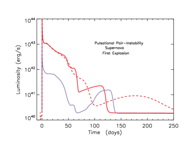
Figure 5.— Light curves from pulsational events in Model T115. (Top:) Light curve from the first pulse and ejection of most of the hydrogen envelope. The solid red line is for the standard red supergiant progenitor and the blue line is for a blue supergiant progenitor. The dashed red line shows the effect of using a larger floor to the opacity. After about 80 days most of the luminosity is due to fallback and accretion and is quite uncertain. (Bottom:) 46 years later, two pulses separated by 130 days eject shells that collide with themselves and with the previously ejected envelope producing the light curve shown. The solid curve is the standard model. The dashed curve results if the velocity of the leading edge of pulse 2 is increased by 50% (see text).

Forty-six years later, after ejecting most of its envelope, Model T115 experienced a second stage of thermonuclear instability during which two additional shells of 5.6 $M_{\odot}$ and 3.5 $M_{\odot}$ were ejected in an interval of 130 days. This added a kinetic energy of $8.9\times 10^{50}$ erg - $5.3\times 10^{50}$ erg in the second pulse and $3.6\times 10^{50}$ erg in the third. The leading edge of pulse 2, located in hydrogen-rich matter (X_H = 0.2, X_He 0.8), initially moved at about 6500 km s^-1. Its interaction with the slower moving material from the prior envelope ejection with speeds $\sim 300-500$ km s^-1 at a radius of $\sim 10^{16}$ cm produced an enduring luminosity $\sim 10^{42}$ erg s^-1 (Fig. 5).

These values are again in the ballpark of the analytic model (§ 2.1), but the velocity and CSM density are too low. The “CSM” comes again from the first pulse and, though 10.6 $M_{\odot}$ was ejected, at the time of the second pulse, only 0.1 $M_{\odot}$ was within $5\times 10^{16}$ cm moving with a speed less than $\sim 300$ km s^-1. 0.3 $M_{\odot}$ was within $1.2\times 10^{17}$ cm with a speed less than 700 km s^-1. This is too little by a factor of about three. The density near the supernova would have been higher if the initial pulse had less energy, if the mass of the envelope were greater, or if the interval between pulses 1 and 2 was shortened. The outer 0.1 $M_{\odot}$ of shell 2 initially moved at 6700 km s^-1 and the outer 1.0 $M_{\odot}$ had a kinetic energy of $2.7\times 10^{50}$ erg and an average speed of 5200 km s^-1. This is again too slow by about 50%.

During the interval between pulses 2 and 3, the leading edge of pulse 2 moved to a radius of $6\times 10^{15}$ cm. Meanwhile, the third pulse, with a leading edge speed near 4000 km s^-1, overtook the slower moving ejecta from the second pulse, producing the bright delayed peak in the light curve (Fig. 5). The integral of the light radiated over the period shown was $2.4\times 10^{50}$ erg, showing the efficient conversion of the kinetic energy of the second and third pulses into radiation. This is also the total light observed in iPTF14hls and that is a success of the model. A better treatment of the radiation transport is needed before anything definitive can be said about the spectrum, but one should note the presence, after the third pulse, of two shells bounded by two shocks with different characteristic speeds not so different from what was observed, 6000 km s^-1 and 4000 km s^-1.

Reasonable adjustments to the model can bring the light curve and hydrogen velocity more in line with observations. Increasing the velocity by 50% in the outer ejecta of pulse 2, just the part moving over 4000 km s^-1, adds $6.2\times 10^{50}$ erg to the kinetic energy of that pulse and gives the modified light curve in Fig. 5. The shock speed at the outer edge of pulse 2 in hydrogen-rich material now declines from 9000 km s^-1 on day 100 to 7200 km s^-1 on day 600, similar to what was observed. The shock bounding pulse 3 decreased in speed from 4000 km s^-1 to 3000 km s^-1 during the same period, also consistent with observations.

Figure 6.— Velocity and density near peak emission in Model T115 (Fig. 5).

Like B120, Model T115 is a reasonable approximation to iPTF14hls if one is allowed a significant modification of the energy of the second pulse. Several potential deficiencies remain though. The separate 4000 km s^-1 component does not appear until after the third pulse and has a different history than the 8000 km s^-1 component. The supernova was not spectroscopically sampled during the first 100 days though, so perhaps this is not a problem, but the overall curve is still too smooth. The integral under the light curve is right, but its shape is wrong. This may reflect deficiencies in the 1D model. In addition to the symmetry breaking conditions mentioned for Model B120, the matter though which the shock generated by pulse 3 passes in Model T115 has experienced mixing due to the Rayleigh-Taylor instability (Chen et al., 2014). It may be clumpy and have angular and radial variations. These would act both to broaden the peak and make the light curve more irregular.

3.2. Models With Shorter Delays and Prompt Black Hole Formation

PPISN models that produce long lasting light curves like iPTF14hls were all previously supernovae that ejected most of their envelope in a bright display. iPTF14hls is made by subsequent pulses running into that ejected envelope and into each other. Envelopes that were ejected more recently (well after 1954) have expanded less and have a greater $q=M_{\rm CSM}/(4\pi R_{\rm CSM})$ in eq. 8. CSM interaction will more easily give a brighter light curve. Also the lower mass leads to more pulses within the duration of the light curve, giving a more irregular history resembling iPTF14hls.

Consider Model T115A of Woosley (2017a, Table 1 here). Despite the similarity in name, this was a different 115 $M_{\odot}$ star than Model T115 in § 3.1.2. Its helium core was 50.47 $M_{\odot}$ instead of 52.93 $M_{\odot}$ and its hydrogen envelope, more massive, 29 $M_{\odot}$. The initial explosion was thus more tamped and the envelope expanded slower. The model had three pulses. The first one (actually a pair of pulses in quick succession) ejected most of the hydrogen envelope with a kinetic energy of $4.55\times 10^{50}$ erg, leaving a remnant of 53.1 $M_{\odot}$, including about 2.6 $M_{\odot}$ of hydrogen envelope. The initial light curve (not shown) resembled the first explosion in Fig. 5. 630 days later, a second strong pulse ejected an additional 5.4 $M_{\odot}$ with kinetic energy $4.05\times 10^{50}$ erg. This included the residual hydrogen envelope plus the outer edge of the helium core. 815 days after that, a third and final pulse ejected an additional 2.0 $M_{\odot}$ of helium core with kinetic energy $2.3\times 10^{50}$ erg. The total kinetic energy in all three pulses was thus $1.09\times 10^{51}$ erg, about $4\times 10^{50}$ erg of which was radiated away in the light curve (Fig. 7). 77 days after this final pulse the star’s iron core collapsed, probably to a black hole, while the light curve was still in progress (at 890 days in Fig. 7).

The initial rise in Fig. 7 is due the second pulse encountering the inner edge of ejected envelope at a radius of $\sim 10^{15}$ cm. The sharp peak about 200 days later is not a new pulse, but the same pulse encountering a thin shell of material piled up by the reverse shock from the first pulse. In reality, this shell would have mixed and not be so thin. The peak at 200 days would be broader, but contain the same radiated energy. The third and final pulse happened at day 815 on the plot, and an additional spike is generated at day 1490 when the piled up shell from pulse 2 running into pulse 1 is encountered by pulse 3. At this point, the core has already collapsed and, baring additional activity generated by compact object formation, no more mass ejection occurs.

The rapid variability in this light curve resembles that of iPTF14hls, though it is perhaps too variable and lasts too long. Mixing in the ejecta would greatly reduce the variability (Chen et al., 2014). Smoothing by $\delta t/t\lower 0.43057pt\hbox{\hbox to0.0pt{\raise 2.58334pt\hbox{\hskip 1.29167pt{{$\scriptscriptstyle>$}}}\hss} \kern-1.72218pt{{$\scriptscriptstyle\sim$}}}$ 10% is reasonable, and would improve the agreement with observations. Shortening the interval between pulses 2 and 3 by a factor of two also leads to a light curve more like iPTF14hls (the dashed line in Fig. 7). This is also a reasonable adjustment, given that the core temperature following pulses, to which neutrino cooling is very sensitive, may not be precisely determined. Typical speeds in the colliding shells are 2000 - 4000 km s^-1 though. This might be adequate to explain the “slow” component seen in the iron lines of iPTF14hls, but no hydrogen moved faster than 5000 km s^-1. Despite many attractive features, baring some additional input of energy (e.g., § 3.3), this model is ruled out by the lack of high velocity hydrogen.

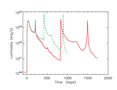
Figure 7.— Light curve for another 115 $M_{\odot}$ model (T115A of Woosley (2017a)) with a larger envelope envelope mass and slightly smaller helium core. The unmodified model (solid red line) experiences repeated outbursts over a 5 year period. The peaks at 0 and 810 days correspond to the second and third pulses in the model. Spikes at 200 and 1490 days are result from the interaction of these pulses with thin shells of previously ejected matter (see text). The iron core collapsed on day 890. The dashed green line shows the result if the interval between pulses 2 and 3 is artificially decreased by a factor of two by increasing the core neutrino losses. Sharp spikes in the light curve would be broadened by at least 100 days by mixing in a two-dimensional calculation. While long lasting, the hydrogenic shock moved too slowly in these models to be iPTF14hls.

Model T110A was similar, but because of its lower helium core mass, the pulses occurred in more rapid secession, resulting in a light curve that was more continuous. The helium core mass was 49.7 $M_{\odot}$, surrounded by an envelope of 20 $M_{\odot}$. A first pulse ($4.72\times 10^{50}$ erg) ejected the hydrogen envelope 10 years prior to a final two pulses that, in rapid succession, ejected an additional 5.2 $M_{\odot}$ of mostly helium with an additional $2.88\times 10^{50}$ erg. Collision of the ejected matter with the inner edge of the previously ejected envelope, which initially had a speed of only a few hundred km s^-1, gave the fainter light curve in the first panel of Fig. 8. The model glowed continuously with supernova-like luminosity for over 1000 days. Typical interaction radii were 0.6 to $2\times 10^{16}$ cm. Over the course of the light curve, the shock speed declined from 4000 km s^-1 to 1600 km s^-1. Most of the time it was near 2000 km s^-1. The velocity of the hydrogen just outside the shock was $\sim$1000 km s^-1.

This shock speed is far too slow, and the light curve too faint to be iPTF14hls. A brighter, shorter (but still 700 days long) light curve results if the velocity of the matter ejected by this second set of pulses is increased by a factor of 1.5 corresponding to an energy increase of $3.5\times 10^{50}$ erg, well within reach of the PPISN model. Now the shock speeds are 6000 to 3200 km s^-1, but the higher speed only lasts a short time and may not have been observed.

Model T110A is not unique. The second panel in Fig. 8 shows that Model T110B, with essentially the same helium core mass, 49.50 $M_{\odot}$, but larger envelope mass, 34 $M_{\odot}$, has a similar light curve. Apparently when stars with the right helium core mass, roughly 50 to 55 $M_{\odot}$ for the physics in the KEPLER code, die in stars with substantial envelopes, they frequently make supernovae that resemble iPTF14hls.

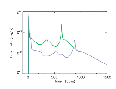
Figure 8.— Top: Explosions of 110 $M_{\odot}$ PPISN corresponding to Models T110A (top frame) and T110B (bottom frame) of Woosley (2017a) In the top frame the green curve results if the velocity is multiplied by 1.5.

In summary, lighter models that do not attempt to explain the 1954 transient also give light curves that, with minor adjustments, agree with the brilliance, duration, and variability of iPTF14hls. They can also explain the time history seen in the iron lines. Unfortunately, all models examined so far fail to give the high velocity seen throughout the event for the Balmer lines of hydrogen. In this regard, they do even less well than the longer duration, more energetic events that might also explain the 1954 transient (§ 3.1).

3.3. Anisotropic Models with Terminal Explosions

All PPISN models thus far have been one-dimensional and each has assumed the formation of an inert black hole once pulsational activity ceases. With the additional freedom of angular dependence and the added energy of a terminal explosion, one can construct a broader range of models, invoking disparate conditions at different angles for the low and high velocity components. It becomes easier to make high velocity hydrogen.

The chief uncertainty here is how an energetic, anisotropic flow would develop in a thermonuclear model that is inherently isotropic. Rotation is the obvious explanation. There is adequate angular momentum in some PPISN models for the iron core to become a millisecond magnetar, though such models must avoid ever becoming supergiants (Woosley, 2017a). It would be very hard though to reverse the inflow of collapse and eject everything outside the neutron star. One would also expect 40 $M_{\odot}$ of oxygen and heavy elements to eventually make their presence known. For the time being, if a terminal, anisotropic explosion is to occur in a PPISN, it seems more natural to invoke black hole formation. The black hole would have a mass of about 45 $M_{\odot}$ and could be rotating rapidly with a Kerr parameter $\sim 0.1$. Polar outflows could develop from the accretion of even a small amount of matter (MacFadyen et al., 2001; Quataert & Kasen, 2012; Woosley & Heger, 2012; Dexter & Kasen, 2013), provided the necessary magnetic fields could be generated near the event horizon of the rapidly rotating hole. Accreting 0.1 $M_{\odot}$ with 1% efficiency for conversion of rest mass into outflow could power a 10⁵¹ erg outflow. It is interesting that this would make iPTF14hls a close relative of gamma-ray bursts, with similar energy, but greater baryon loading and perhaps less collimation. The main difference here, aside from the large black hole mass, is the presence of solar-mass shells of matter with which the accretion energized outflow can interact.

Besides the uncertain physics of such a terminal explosion, there is the issue of its timing. For two components to appear in the spectrum of the same event, they must commence close together. Iron-core collapse needs to follow swiftly on the heels of the final pulses. There are PPISN where this is the case, though there usually at least a few week’s delay as the star goes through a final stage of stable silicon shell burning (Table 1). There is also an issue of how to input the energy from a terminal explosion into the code. If it comes from polar outflows driven by accretion on a massive black hole, the energy might be in the form of a small mass moving at semi-relativistic speed. Retaining the kinetic energy of this small mass and not promptly radiating it away as something resembling a gamma-ray burst afterglow requires that the shells with which it interacts still be optically thick.

Consider Model T110A (Fig. 8;§ 3.2) that ejected most of its hydrogen envelope 12 years before two final pulses and the collapse of its iron core (Table 1). Unfortunately in that model iron-core collapse did not occur until 830 days after the last pulse. Adding a high velocity component in just the final few hundred days would not explain the observations. In Model T110B, the delay between the final pulse and core collapse was just 55 days. The difference was a slightly higher central temperature, $1.36\times 10^{9}$ K versus $1.13\times 10^{9}$ K immediately after the pulses. A high velocity component in Model T110B, however, gave too bright and too brief a light curve because the hydrogen envelope had not expanded enough. The first supernova was too close to core collapse. Model T115B (Woosley, 2017a) had a strong final pulse just 12 days before core collapse. It’s inner solar mass had already turned to iron after that pulse, so silicon shell burning was of limited duration.

In order to show what might happen in a model capable of producing comparable luminosities in the large angle and polar outflows, attention was focused on Model T110A. Energetic explosions were introduced just 10 days after the final pulse Fig. 8. These were not explosions of the core though. The remaining 44.6 $M_{\odot}$ core was excised, presumably to make the black hole, and 0.1 $M_{\odot}$ of the matter in the inner edge of the last shell to be ejected given a high speed corresponding to a energies of 24, 12, and 6 $\times 10^{51}$ erg. Since this was a one-dimensional simulation, these are the equivalent isotropic energies, that are really assumed to pertain to just some small solid angle, assumed here to be 10% of the sky. So the 12 $\times 10^{51}$ erg case, for example, only requires an energy input of $1.2\times 10^{51}$ erg.

The resulting light curves are shown in Fig. 9. They are very bright. Just 10% of the luminosity of the 12 $\times 10^{51}$ erg model could power the observed light curve of iPTF14hls and then some. The velocity history (Fig. 9) is also in reasonable agreement with what was observed for the H_α line, especially if the event was not observed in the first 100 days. The small mass of hyper-velocity ejecta impacts the two shells ejected by the final two pulses and sweeps them up. Because the collision occurs in a region that is still marginally optically thick, kinetic energy is conserved and not promptly radiated away. Models in which the energy was injected at day 60 fared less well and only the most energetic case retained enough kinetic energy after the break out transient to power a light curve like iPTF14hls - again assuming a solid angle of 10% of the sky.

In summary, a two component PPISN model with a terminal explosion is contrived, but could potentially explain the major features of iPTF14hls. The model requires both the production of a mildly relativistic jet, for which a physical basis is lacking, and that the core collapse very shortly after the last pulse of the PPISN. A similar model was proposed by Woosley (2017a) to explain superluminous supernovae, but there the timing of the core collapse was not so constrained by the need to produce a long light curve with constant velocity components. Also, in the models of Woosley (2017a), the entire helium and heavy element core within the given solid angle was ejected, not just a small mass outside a black hole.

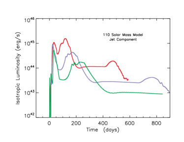
Figure 9.— Top: Light curves of three very energetic explosions perhaps powered by black hole accretion. The explosions were initiated by giving a small amount of mass a very high speed and allowing it to impact on the shells ejected in Model T110A (see Fig. 8). The explosions had equivalent isotropic energies of 24, 12, and 6 $\times 10^{51}$ erg. The amount of energy radiated as light in the three models was 15, 7.2, and 3.6 $\times 10^{51}$ erg. These energies and the luminosity in the figure should be multiplied by the fraction of the sky subtended by the mildly relativistic outflow, perhaps $\sim 10$%, and added to the luminosity for Model T110A in Fig. 8. (Bottom:) Velocity and density in the $7.2\times 10^{51}$ erg explosion (blue line in top panel) evaluated at 120, 180, 440, and 730 days on the light curve plot.

4. Magnetar Models

Magnetars are neutron stars with unusually strong magnetic fields compared with radio pulsars. Typically a magnetar has a (dipole) field strength  $\scriptscriptstyle>$ $\scriptscriptstyle\sim$10¹⁴ G. The strong magnetic field of the neutron star, in theory, is a consequence of very rapid rotation at the time of its birth (Duncan & Thompson, 1992). The existence of magnetars and their key role in explaining soft gamma-ray repeaters and anomalous x-ray pulsars is beyond doubt (Kaspi & Beloborodov, 2017). The time during which the magnetar shines brightly is short compared with pulsars and, given their numbers and spatial distribution, more than 10% of all neutron stars are probably born with these strong fields and, presumably, rapid rotation. Rapidly rotating magnetars are also the central engine in a leading model for gamma-ray bursts (e.g. Usov, 1992) where they are required to have magnetic fields greater than 10¹⁵ G and powers $\lower 0.43057pt\hbox{\hbox to0.0pt{\raise 2.58334pt\hbox{\hskip 1.29167pt{{$\scriptscriptstyle>$}}}\hss} \kern-1.72218pt{{$\scriptscriptstyle\sim$}}}10^{50}$ erg s^-1. Somewhere between these extremes of rotation rate and field strength - ordinary pulsars and ultra-powerful magnetars, $B\sim 10^{14}$ G and P $\sim$ few ms should exist. For such characteristics, a light curve like iPTF14hls is a natural consequence.

For lack of a deeper understanding, the magnetar energy and power of a magnetar just after its birth are generally approximated using the same two-parameter equations as employed for much older pulsars:

$$\begin{split}E&=\frac{1}{2}I\omega^{2}\\ &\approx 2\times 10^{52}{\rm P}_{\rm ms}^{-2}\ {\rm erg}.\end{split}{}$$ (9)

where $E$ is the rotational energy, $I$, the moment of inertia ($\approx 10^{45}$ g cm²), and $P_{\rm ms}$, the period in ms. The approximate energy loss for dipole radiation is given by the Larmor formula (e.g., Lang, 1980),

$$\begin{split}\frac{dE}{dt}&=\frac{2}{3c^{3}}\left(BR^{3}\ {\rm Sin}\,\alpha\right)^{2}\left(\frac{2\pi}{{\rm P}}\right)^{4}\\ &\approx 10^{49}B_{15}^{2}{\rm P}_{\rm ms}^{-4}\ {\rm erg\ s^{-1}}.\end{split}{}$$ (10)

Here $B_{15}$ is the surface dipole field in 10¹⁵ Gauss, $R\approx 10^{6}$ cm is the neutron star radius, and $\alpha$ is the inclination angle between the magnetic and rotational axes, taken arbitrarily to be 30 degrees. These equation may be integrated to give the energy and power at time $t$ (Woosley, 2010),

$$\begin{split}\frac{dE}{dt}&=\left(\frac{dE}{dt}\right)_{0}\left(1\,+\,t/t_{p}\right)^{-2}\\ E&=E_{o}\\ t_{p}&=2000\,P_{ms0}^{2}B_{15}^{-2}\ {\rm s}\end{split}{}$$ (11)

Similar equations have been given by Kasen & Bildsten (2010) with a different choice of inclination angle. Their equations are recovered if $B$ in the above equations is divided by $\sqrt{2}$.

These equations have the simplicity of a physical model that can be adjusted using the two parameters to fit almost any smooth light curve so long as the emitted radiation and wind is thermalized inside the expanding star and emitted chiefly in the optical. They are too simple however, especially at very early times, when the neutron star and its crust are rapidly evolving. The same magnetic field and rotation needed to eject the accreting matter and power the supernova, a power of at least 10⁵⁰ erg s^-1 (more if appreciable ⁵⁶Ni is to be synthesized), would rapidly sap the rotational energy and leave the magnetar powerless during the months needed to power the light curve. Thus we expect that $B$ in the above equation is not a constant at early times.

Given that iPTF14hls was already well underway when discovered, one must also include an element of uncertainty as to just when the core collapsed and started the event. The magnetar may have deposited appreciable energy before the supernova was discovered.

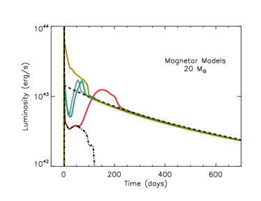
Figure 10.— Light curves and terminal velocities for a supernova derived from a 20 $M_{\odot}$ model (Table 1) with several varieties of magnetars embedded. The brief display represented by the dot-dashed line in the light curve figure is a normal 20 $M_{\odot}$ supernova model with regular mass loss and no embedded magnetar. The dashed line is the dipole power radiated by a magnetar with initial rotational energy 0.6 $\times 10^{51}$ erg and magnetic field strength $4\times 10^{13}$ G according to eq. 11. The colored curves show the result of embedding this fiducial magnetar in four different supernovae with different mass loss histories and energy deposition during their first 10,000 s (see text for discussion). The lower panel shows the terminal velocity for the same four supernovae. Models A and B have a constant magnetic field and a normal supernova energy. Models C and D have a time varying field that produces a more powerful explosion early on.

Arcavi et al. (2017) found a good overall fit to the light curve of iPTF14hls using the formulae of Kasen & Bildsten (2010) with B = $7\times 10^{13}$ G and an initial rotational period of 5 ms (E = $8\times 10^{50}$ erg). Using eq. 11 gives a similar good fit for an initial rotational energy of $6\times 10^{50}$ erg and B = $4\times 10^{13}$ G. Fig. 10 and Table 1 show the result when a magnetar with these properties is embedded in a supernova derived from a star with solar metallicity and a mass of 20 $M_{\odot}$ on the main sequence. With a normal mass loss rates, the star had a total mass of 15.93 $M_{\odot}$ at death. The helium core mass was 6.17 $M_{\odot}$ and the rest of the star was a low density, hydrogen-rich envelope. The star was a a red supergiant with luminosity $5.7\times 10^{38}$ erg s^-1 and radius $7.42\times 10^{13}$ cm. This star, exploded with a piston at 1.82 $M_{\odot}$ (the base of the oxygen shell where the entropy per baryon reaches 4.0), has been previously published in Woosley & Heger (2007). The explosion produced 0.14 $M_{\odot}$ of ⁵⁶Ni and had a final kinetic energy of $1.2\times 10^{51}$ erg. The light curve of this rather standard SN Type II-P model is shown as the dot-dashed line in Fig. 10.

For Model 20A in Fig. 10, the red line with the broad peak at 150 d, is the light curve that results when power from the standard magnetar defined above, shown as the dashed line, is embedded in this model. Somewhat like the radioactive peak in SN 1987A, the bottled up magnetar energy diffuses out producing a delayed peak. Once that wave of radiation diffuses out, the bolometric light curve just reflects the magnetar power with no delay. Even though the bolometric light curve is not badly represented if, say, the SN was discovered after 200 d, the low velocity shown as the red line in the second panel of Fig. 10 is much slower than the speeds observed in iPTF14hls.

Better agreement with spectral constraints is achieved if the presupernova star has lost most of its hydrogen envelope before exploding (Model 20B in Fig. 10 and Table 1). The expansion of the helium core is then not so tamped by and the small mass of envelope expands with a higher speed. This particular model had a mass loss rate 3 time the standard value and ended with a total mass of 7.41 $M_{\odot}$, a helium core mass of 5.83 $M_{\odot}$, and a hydrogen envelope of 1.58 $M_{\odot}$. It was exploded with a piston at 1.58 $M_{\odot}$ and had a final kinetic energy of $1.1\times 10^{51}$ erg. Without an embedded magnetar, the light curve of this model (not shown) is brief and just a bit brighter than the standard explosion, essentially the green curve in Fig. 10 before the rapid rise at $\sim 25$ d. With the standard magnetar (0.6 $\times 10^{51}$ erg, $4\times 10^{13}$ G), the light curve is similar to Model 20A, but due to the smaller mass envelope, the bump from magnetar break out is fainter and happens earlier. This could reduce the delay time between explosion and discovery. The velocity in outermost part of the ejected hydrogen envelope now exceeds the 8000 km s^-1, but only in 0.3 $M_{\odot}$. It might be difficult for this small mass to dominate the spectrum for 600 days. The speed of the helium and heavy element core is faster than in Model 20A, but still substantially slower than 4000 km s^-1.

While other radii, masses of stars, explosion energies, and magnetar properties could be explored, the properties for this one 20 $M_{\odot}$ model are probably generic. Without greatly increasing the explosion energy, the helium core will not move much faster. The magnetar properties are essentially fixed by observations after break out. The radius only affects the initial light curve and, to some extent, the peak velocity of the ejecta. Something else may be needed to explain the constancy of of H_α and iron speeds in the spectrum.

The missing ingredient could relate to the assumption of a constant magnetic field strength throughout the supernova’s evolution. Consider a case where the magnetar field strength is much greater early on and the initial rotational energy is not a perturbation on some other undefined energy source, but actually the cause of the explosion. During its first 100 - 1000 s, and especially its first 10 s, the magnetar will still be evolving rapidly. Damping of the initial differential rotation and neutrinos may have already launched a successful explosion (Akiyama et al., 2003), but the magnetar continues to deposit considerable energy after that adding to the kinetic energy of the explosion. A relevant time scale for the supernova is the shock crossing time for the helium core, about 100 s. A relevant time for the neutron star might be the interval necessary for the crust to form, typically estimated at minutes to hours (Sanjay Reddy, private communication). Perhaps the neutron star forms with a powerful field generated by convection which then decays until the crust forms and a residual field is “locked in”?

To explore this speculation, the explosion of the same 20 $M_{\odot}$ star was modeled assuming a large magnetic field, $2\times 10^{15}$ G during the first 10⁴ s, but only $4\times 10^{13}$ G thereafter. The initial rotational energy of the neutron star was either $2\times 10^{51}$ erg (Model 20C) or $15\times 10^{51}$ erg (Model 20D), but in both cases, that rotational energy has decayed to about $6\times 10^{50}$ erg after 10⁴ s. In the high energy case half of the initial energy was deposited in 650 s. In the low energy case, half the energy was deposited in 5000 s. The actual time scales are not so relevant so long as: a) most of the energy is deposited in a few helium core expansion time scales, and b) the neutron star retains $6\times 10^{50}$ erg of rotational energy after a few weeks.

For the lower energy case, Model 20C, the light curve for the progenitor with the low mass hydrogen envelope (1.58 $M_{\odot}$) was very similar to the case with constant magnetic field, Model 20B, the blue and green light curves in Fig. 10. Doubling the final kinetic energy does not greatly affect the light curve, but the velocity profile is changed in an interesting way. The hydrogenic envelope expands only slightly faster, but the helium and heavy element core moves much faster, at a nearly constant speed close to 4000 km s^-1. This reflects the fact that the energy deposited in the core after the initial shock has exited is greater that from the shock itself. As a result the entire core is compressed into a thin shell. The inner 2 $M_{\odot}$of ejecta moves with speeds between 4200 and 4400 km s^-1. By 10⁷ s when the explosion is well into the coasting phase, the entire helium and heavy element core (4.1 $M_{\odot}$ of ejecta) is compressed into a shell with radius $4.2-5.5\times 10^{15}$ cm moving at 4200 to 5500 km s^-1 (Fig. 11). If this shell were ionized, which it was not in the present study, perhaps due to an overly simple treatment of radiation transport, it would be optically thick.

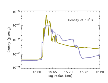
Figure 11.— Density at 10⁷ s for the ejected material contained in the former helium and heavy element core. The blue curve is for Model 20C and the brown curve for Model 20D. In both cases, the magnetar has inflated a bubble of radiation and pushed the ejected helium and heavy elements into a thin shell coasting with nearly constant velocity. Fast moving hydrogen outside has a lower density. These profiles scale as 1/t³ with t the elapsed time greater than 10⁶ s.

Having opened the door to the possibility of a time-varying field, it is interesting to explore the limits. Arcavi et al. (2017) suggest that a kinetic energy of order 10⁵² erg and a mass $\sim$10 $M_{\odot}$ is needed to explain the evolution of the Balmer lines in iPTF14hls. As Model 20C in Fig. 10 shows, even $2\times 10^{51}$ erg is inadequate to give the high observed speeds if progenitor explodes with a large envelope mass. Model 20D retains the large envelope mass and the fiducial low energy magnetar after 10⁴, but during the first 10⁴ s incorporates a magnetar with an initial rotational energy of $15\times 10^{51}$ erg (1.2 ms period) and magnetic field strength $2\times 10^{15}$ G. Now the hydrogen envelope moves faster and now its average speed is near 8000 km s^-1, although with a wide spread. That part of the helium and heavy element core that did not end up in the neutron star all moves at a nearly constant 4000 km s^-1 in a thin shell with high density contrast (Fig. 11). In the KEPLER calculation, the large radius of this matter implies a temperature below that required to ionize helium and the electron scattering opacity is low, but if this material had an effective opacity near 0.1 cm² g^-1 this shell would be marginally optically thick at 10⁷ s. Matter outside log r = 15.73 in Model 20C and log r = 15.65 for Model 20D and in Fig. 11 is hydrogen rich.

In summary, given the liberty to adjust the explosion time, the overall fit to the bolometric light curve is pretty good for all the magnetar models, though the 1D simulations have difficulty explaining multiple peaks in the observations. These peaks might be a consequence of instabilities at the boundary of the “bubble” created inside the expanding supernova by the magnetar radiation and wind. This boundary is known to be Rayleigh-Taylor unstable resulting in a clumpy filamentary structure (Chen et al., 2016; Kasen et al., 2016; Blondin & Chevalier, 2017). While this shell remains optically thick, the escape of radiation could be irregular. Alternatively the magnetar itself might experience “superflares” (Kaspi & Beloborodov, 2017), but, to explain a peak with integrated luminosity $\sim 10^{49}$ erg, these flares would need to be about 1,000 times more energetic than ever seen before, e.g. in the event of March 5, 1979. Both these possibilities are speculative and would need to be reinforced by future studies, e.g., of the light curve for a multi-dimensional model.

A major problem though with the magnetar models considered here is that the slowest moving hydrogen in all but the high mass, low B-field case (Model 20A) is above 3500 km s^-1. Mixing might reduce this value somewhat for Model 20B, but the need to have both 8000 km s^-1 hydrogen the first 600 days, which rules out Model 20A, and 1000 km s^-1 hydrogen at late times (Andrews & Smith, 2017), is highly constraining.

5. Conclusions

The most likely explanations for iPTF14hls involve CSM interaction or magnetar birth. For CSM interaction, the event’s long duration is a consequence the large radius, $\sim 5\times 10^{16}$ cm, of the CSM, and relatively mild speed of the supernova ejecta. For magnetars, the duration reflects the lengthy spin-down time for a neutron star with a moderate field strength, $B\sim 4\times 10^{13}$ G.

Indeed, continuous emission lasting 600 days or more at 10⁴² - 10⁴³ erg s^-1 (bolometric), perhaps the defining characteristic of iPTF14hls, is easily achieved in a variety of models, including an ordinary supernova happening in a dense CSM medium (§ 2; Andrews & Smith, 2017); PPISN (§ 3; Arcavi et al., 2017; Andrews & Smith, 2017; Woosley et al., 2007; Woosley, 2017a, b); and magnetar-based models (§ 4; Arcavi et al., 2017). See Figures 1, 4, 5, 7, 8, and 10. Satisfying the spectroscopic constraints is more difficult.

Generic models for CSM interaction (§ 2.1) require a circumstellar mass of about 0.4 $M_{\odot}$ with an outer radius of $5\times 10^{16}$ cm interacting with an ejected shell with 1.0 $M_{\odot}$ and kinetic energy near $5\times 10^{50}$ erg. The velocity of the shock at the interface in this fiducial model would be 6500 km s^-1 (eq. 5) after 600 days. At late times, the luminosity would decline as $t^{0.3}$ (eq. 8) and the velocity, as $t^{-0.1}$, but both these scaling relations depend upon uncertain density distributions in the ejecta and CSM and could vary with time. Early on, one would expect narrow lines in the spectrum characteristic of the CSM, but the pile up of matter in a dense shell moving with the shock speed into an optically thin medium might result in the higher velocity dominating the spectrum. The light curve in Fig. 1 assumes a CSM density that varies smoothly as $r^{-2}$. Irregularities in the mass loss rate or angle dependence would be required to give structure to the light curve.

Providing a CSM of order 0.4 $M_{\odot}$ at a few $\times 10^{16}$ cm may be difficult for binary interaction models or wave-driven mass loss. The necessary time scale for the ejection is unnaturally short for the former and long for the latter. An exception is a star with mass near 10 $M_{\odot}$ that ejects its hydrogen envelope a couple of years before core collapse (Woosley & Heger, 2015), but the explosion energies of such low mass stars may be inadequate to produce the observed light curve (Sukhbold et al., 2016).

The origin of distinct spectroscopic components at 4000 and 8000 km s^-1 is not clear in the simplest spherically symmetric CSM interaction model, though calculations of the spectra of e.g., the model in Fig. 2 are needed to address this issue. One could envision relatively minor modifications to the circumstellar mass density (Andrews & Smith, 2017), mass loss history, or supernova central engine that would give asymmetric models with the different velocities coming from ejecta at different angles. Conceptually, despite their uncertainties, these CSM models are the simplest explanation for iPTF14hls.

PPISN, which are just an extreme case of CSM interaction, also have several attractive features (Arcavi et al., 2017; Andrews & Smith, 2017; Woosley, 2017b). Numerous non-rotating models with masses 105 - 120 $M_{\odot}$ are capable of producing continuous light curves with supernova-like brightnesses lasting over 500, or even 1500 days (Table 1; Figures 4, 5, 7, and 8). The total energy radiated in light in these models, $2-3\times 10^{50}$ erg, is the same as in iPTF14hls, Some of the models, e.g., Fig. 8 show variability due to multiple pulsations and collisions with piled up material from previous pulses. Others are capable of producing transients decades before iPTF14hls, possibly even a transient in 1954 (Fig. 5; § 3.1). Each PPISN model could, with minor modification, produce the characteristic 4000 km s^-1 seen in the iron lines of iPTF14hls. Some, with multiple pulses, could also produce multiple spectroscopic components (Fig. 6). All should occur preferentially in star forming regions with low metallicity. The physics of their explosion is simple compared with neutrino transport or magnetar birth. They are a phenomenon that must happen in nature provided only that stars die with the necessary helium cores masses, 50 - 54 $M_{\odot}$ in this case. But no one model, here at least, does it all.

In defense, PPISN are difficult to match to individual events. Their repeated outbursts amplify small differences in the initial model. The pair neutrino loss rate at 10⁹ K, a relevant post-pulse temperature, depends on temperature to the 14th power. Slight variations in the temperature following a pulse, due e.g., to a minor change in the amount of fuel burned in the previous pulse, have big effects on the intervals between pulses and the light curve. Convective mixing in the core between pulses causes some uncertainty - when to mix and at what rate. The passage of shock waves through the outer layers of the helium core leaves the matter that falls back and remains bound in a state of thermal disequilibrium. Since the temperature there is too cool for neutrino emission, the matter remains stuck in a distended state (Fig. 12) that might not be accurately calculated in one dimension. Both the interpulse period and shock hydrodynamics are sensitive to the density distribution in this matter. For these reasons, the interval between pulses and pulse energies were sometimes adjusted in this paper to explore the consequences.

Figure 12.— Density distribution for Model T115 evaluated after the first pulse ejects all matter external to 53.9 $M_{\odot}$ (solid line) and in the presupernova star near carbon depletion (dashed line). The times have been chosen such that the central density is the same $1.6\times 10^{4}$ g cm^-3 in both cases. All matter plotted is in hydrostatic equilibrium and the helium core mass is 52.9 $M_{\odot}$. The outer part of the helium core, e.g., at 50 $M_{\odot}$, is disturbed by the first pulse and remains in an extended state of lower density and larger radius going into pulse 2. The entropy per baryon for the solid line at 50 $M_{\odot}$ (32.9) is twice that of the dashed line (17.3) at the same mass. The density structure of this expanded matter affects the interpulse period and maximum speed developed in pulse 2.

PPISN energies are also relatively anemic. Typical total kinetic energies for the relevant mass range are $0.7-1.5\times 10^{51}$ erg (Table 1), shared among two or three pulses. Even with roughly 50% conversion of kinetic energy to light, it is difficult for PPISN to explain light curves totaling more than a few times 10⁵⁰ erg. The maximum kinetic energy in pulse 2 was $6.8\times 10^{50}$ erg for Model B120 shared by 5.1 $M_{\odot}$ of ejecta. This is adequate for the light curve of iPTF14hls, especially if the interval between pulses 1 and 2 can be adjusted, but too little to boost the necessary solar mass or so of hydrogen-rich material to speeds over 8000 km s^-1. In several cases, increasing the energy of the second pulse by less than 10⁵¹ erg made the difference between an acceptable model and one that lacked sufficient high velocity hydrogen. Given the uncertainties described above, is this a reasonable variation?

The fundamental energy limit on PPISN models, empirically, is that all of the pulses exhaust carbon, oxygen and neon within the inner 5 $M_{\odot}$ of the presupernova star. That is, the silicon plus iron core of a PPISN at iron-core collapse is always near 5 $M_{\odot}$ for stars in the relevant mass range (Woosley, 2017a). Most of that is silicon. The iron that is there is mostly made after the pulses are over. Burning a mixture of 80% oxygen and 20% neon to one of 70% silicon and 30% sulfur generates $4.6\times 10^{17}$ erg g^-1, or about $5\times 10^{51}$ erg for 5 $M_{\odot}$. Most of this energy is lost to neutrinos during the interpulse intervals, but an overall energy budget of $2\times 10^{51}$ erg would accommodate all the artificial modifications made in this paper.

Several varieties of PPISN models were explored, characterized by their potential ability to explain both the 1954 transient and iPTF14hls (§ 3.1); success at making only iPTF14hls (§ 3.2) with a more recent unobserved supernova; and hybrid models that invoked both a PPISN and a terminal explosion (§ 3.3). In the first case, the interval between the beginning of pulsations and iron-core collapse was much longer than the period of pulsational instability. The remnant of the latest explosion would still be a star shining with a luminosity $\sim 10^{40}$ erg s^-1, perhaps for centuries to come. This is probably too faint to detect in iPTF14hls, and might be confused with circumstellar interaction, but worth keeping mind for future discoveries. Other models that did not make the 1954 transient produced a collapsed remnant, presumably a black hole of 40 - 45 $M_{\odot}$, either while the light curve was still active or shortly thereafter. The models that made a transient in 1954 were marginally more successful at explaining both the light curve of iPTF14hls and its high velocity hydrogen without any modification, though none was without flaw. Models that did not attempt to make the 1954 transient had more structure and, in some cases, lasted longer, but were less energetic, and their hydrogen-rich ejecta was slower.

The most uncertain, but potentially exciting class of PPISN models is a hybrid model (§ 3.3) in which a PPISN is accompanied by some sort of asymmetric terminal explosion when the iron core collapses. This terminal explosion could possibly be magnetar formation, which would open up a very broad parameter space, but here the model briefly explored was black hole accretion (see also Dexter & Kasen, 2013; Woosley, 2017a). The black hole would be unusual in that it would be about 45 $M_{\odot}$, and not the usual several solar masses invoked in common supernovae or the collapsar model for gamma-ray bursts. The matter that accretes comes from farther out in the star and might have more angular momentum, though whether that would be adequate to produce a jet remains to be demonstrated. This would need to be a subset of an already rare model where the collapse to iron core occurred within a month or so of the final pulses of the pair instability.

Given the necessary condition of previously ejected shells within 10¹⁵ cm being impacted by a polar outflow with equivalent isotropic energy near 10⁵² erg, a very luminous display is generated with high characteristic speeds (Fig. 9). A solid angle of 10% with actual explosion energy near 10⁵¹ erg might suffice to explain the high velocity component of iPTF14hls.

If powered by a magnetar, the light curve and kinematics of iPTF14hls favor a star with a large energy to envelope mass ratio, i.e., Models 20B, 20C, or 20D, but not 20A (Table 1). That is, the star needs to have lost most of its hydrogen envelope or experienced a very energetic explosion. In moderately energetic explosions, even for stars with low mass envelopes, the mass of hydrogen moving over at 8000 km s^-1 was small (e.g., 0.3 $M_{\odot}$ in Model 20B) and might have difficulty substantially impacting the spectrum for 600 days (Arcavi et al., 2017). The presence of two characteristic speeds, 4000 km s^-1 for the iron lines and 6000 - 8000 km s^-1 for hydrogen is suggestive, though not proof, of two different velocity scales in the problem.

A novel magnetar model was explored in which the neutron star was born rotating very fast, but with a strong magnetic field that decayed appreciably during the first few hours of its life. The delayed energy injection resulted in the entire ejected core of helium and heavy elements piling up in a relatively thin shell moving with constant speed $\sim 4000$ k s^-1. Velocities in the hydrogen envelope exceeded 8000 km s^-1 in a substantial fraction of the mass. In any magnetar model though, the need for high velocity hydrogen during the first 600 days and 1000 km s^-1 hydrogen at late times (Andrews & Smith, 2017) is problematic.

Further observations and calculations will help to clarify the actual nature of iPTF14hls. The three models predict very different remnants currently at the supernova site. CSM interaction in an otherwise ordinary supernova would presumably leave an ordinary neutron star in a shellular like remnant. PPISN predict either a Wolf-Rayet like stellar remnant with a luminosity of 10⁴⁰ erg s^-1 or a black hole that might be accreting and emitting hard radiation. The most specific predictions come from the magnetar model which predicts, three years after the explosion, a pulsar with a bolometric luminosity of $1.3\times 10^{42}$ erg s^-1, period, 10.5 ms, and field strength, near $4\times 10^{13}$ G. Five years after the explosion, the luminosity and period would be $6.3\times 10^{41}$ erg s^-1 and 12.3 ms. Eventually an appreciable fraction of the power should be radiated in non-optical wavelengths. While the spectrum of a three year old rapidly rotating magnetar is unknown, continued x-ray monitoring at this level is recommended, as we could be witnessing the birth of an anomalous x-ray pulsar or even a ultra-luminous x-ray source.

In the CSM models, which include PPISN, the shock waves generating the light should slow with time and this should be reflected in the spectrum. PPISN models predict a characteristic speed of 1000 - 3000 km s^-1 for the envelope ejected in the first pulse (depending on both the pulse energy and the mass of the remaining envelope). This is intriguing given the evidence for such slowly moving material in spectra at very late times (Andrews & Smith, 2017). The supernova speed would eventually saturate near that value. In a more common supernova, slower speeds characteristic of the pre-explosive wind might eventually appear, but the supernova itself would retain its high speed.

In the PPISN models, the mass that was ejected consists chiefly of hydrogen, helium, carbon, oxygen, nitrogen, neon and magnesium. Heavy elements like silicon, calcium, and iron are confined to what existed in the envelope of the star when it was born. No new iron or intermediate mass elements are ejected. Even in the hybrid models with terminal explosions, the heavy elements are presumed to collapse into the black hole. In an ordinary supernova or magnetar model, heavy elements would have been ejected including a solar mass or so of slowly moving oxygen. Freshly synthesized silicon, calcium, and iron might contribute to the spectrum.

In terms of theory, all of the models presented here would be much more definitive with a better treatment of radiation transport.

References

- Akiyama et al. (2003) Akiyama, S., Wheeler, J. C., Meier, D. L., & Lichtenstadt, I. 2003, ApJ, 584, 954
- Andrews & Smith (2017) Andrews, J. E., & Smith, N. 2017, arXiv:1712.00514
- Arcavi et al. (2017) Arcavi1, U., Howell1, D. A., Kasen, D., Bildsten, L., Hosseinzadeh1, G., et al 2017, submitted to Nature.
- Blondin & Chevalier (2017) Blondin, J. M., & Chevalier, R. A. 2017, ApJ, 845, 139
- Chen et al. (2014) Chen, K.-J., Woosley, S., Heger, A., Almgren, A., & Whalen, D. J. 2014, ApJ, 792, 28
- Chen et al. (2016) Chen, K.-J., Woosley, S. E., & Sukhbold, T. 2016, arXiv:1604.07989
- Chevalier (1982a) Chevalier, R. A. 1982a, ApJ, 258, 790
- Chevalier (1982b) Chevalier, R. A. 1982b, ApJ, 259, 302
- Chevalier (1982c) Chevalier, R. A. 1982c, ApJ, 259, L85
- Chevalier & Fransson (1994) Chevalier, R. A., & Fransson, C. 1994, ApJ, 420, 268
- Dexter & Kasen (2013) Dexter, J., & Kasen, D. 2013, ApJ, 772, 30
- Duncan & Thompson (1992) Duncan, R. C., & Thompson, C. 1992, ApJ, 392, L9
- Fuller (2017) Fuller, J. 2017, MNRAS, 470, 1642
- Fuller & Ro (2017) Fuller, J., & Ro, S. 2017, arXiv:1710.04251
- Kasen & Bildsten (2010) Kasen, D., & Bildsten, L. 2010, ApJ, 717, 245
- Kasen et al. (2016) Kasen, D., Metzger, B. D., & Bildsten, L. 2016, ApJ, 821, 36
- Kaspi & Beloborodov (2017) Kaspi, V. M., & Beloborodov, A. M. 2017, ARA&A, 55, 181
- Lang (1980) Lang, K. R, 1980, Astrophysical Formulae. (Springer Verlag), p. 475
- MacFadyen et al. (2001) MacFadyen, A. I., Woosley, S. E., & Heger, A. 2001, ApJ, 550, 410
- Quataert & Kasen (2012) Quataert, E., & Kasen, D. 2012, MNRAS, 419, L1
- Quataert & Shiode (2012) Quataert, E., & Shiode, J. 2012, MNRAS, 423, L92
- Quataert et al. (2016) Quataert, E., Fernández, R., Kasen, D., Klion, H., & Paxton, B. 2016, MNRAS, 458, 1214
- Sukhbold et al. (2016) Sukhbold, T., Ertl, T., Woosley, S. E., Brown, J. M., & Janka, H.-T. 2016, ApJ, 821, 38
- Sukhbold et al. (2018) Sukhbold, T., Woosley, S., & Heger, A. 2018, ApJ, in press, arXiv:1710.03243
- Usov (1992) Usov, V. V. 1992, Nature, 357, 472
- Weaver, Zimmerman, & Woosley (1978) Weaver, T. A., Zimmerman, G. B., & Woosley 1978, ApJ, 225, 1021
- Woosley et al. (2002) Woosley, S. E., Heger, A., & Weaver, T. A. 2002, Reviews of Modern Physics, 74, 1015
- Woosley et al. (2007) Woosley, S. E., Blinnikov, S., & Heger, A. 2007, Nature, 450, 390
- Woosley & Heger (2007) Woosley, S. E., & Heger, A. 2007, Phys. Rep., 442, 269
- Woosley (2010) Woosley, S. E. 2010, ApJ, 719, L204
- Woosley & Heger (2012) Woosley, S. E., & Heger, A. 2012, ApJ, 752, 32
- Woosley & Heger (2015) Woosley, S. E., & Heger, A. 2015, ApJ, 810, 34
- Woosley (2017a) Woosley, S. E. 2017a, ApJ, 836, 244
- Woosley (2017b) Woosley, S. 2017b, Nature, 551, 173