Abstract

This paper revisits the well-studied fixed point problem from a unified viewpoint of mathematical modeling and canonical duality theory, i.e. the original problem is first reformulated as a nonconvex optimization problem, its well-posedness is discussed based on objectivity principle in continuum physics; then the canonical duality theory is applied for solving this problem to obtain not only all fixed points, but also their stability properties. Applications are illustrated by challenging problems governed by nonconvex polynomial, exponential, and logarithmic operators. This paper shows that within the framework of the canonical duality theory, there is no difference between the fixed point problems and nonconvex analysis/optimization in multidisciplinary studies.

Key Words: Fixed point, properly-posed problem, nonconvex optimization, canonical duality theory, mathematical modeling, multidisciplinary studies.
Mathematics Subject Classification (2010): 47H10, 47H14, 55M05,65K10

1 Mathematical Modeling and Objectivity

The fixed point problem is a well-established subject in the area of nonlinear analysis [2, 3, 6], which is usually formulated in the following form:

$$({\cal{P}}_{0}):\;\;\;\;{\bf x}={F}({\bf x}),$$ (1)

where ${F}:{\cal X}_{a}\rightarrow{\cal X}_{a}$ is nonlinear mapping and ${\cal X}_{a}$ is a subset of a normed space ${\cal X}$. Problem $({\cal{P}}_{0})$ appears extensively in engineering and sciences, such as equilibrium problems, mathematical economics, game theory, and numerical methods for nonlinear dynamical systems. The general form of equilibrium problem was first considered by Nikaido and Isoda in 1955 as an auxiliary problem to establish existence results for Nash equilibrium points in non-cooperative games [37, 38, 39, 40]. Mathematically speaking, the nonlinear operator $F({\bf x})$ could be any arbitrarily given vector-valued function. Therefore, the fixed point problem $({\cal{P}}_{0})$ is artificial. Although it can be used to “model” a large class of mathematical problems, one must pay a price: it is impossible to develop a unified mathematical theory with powerful real-world applications. This dilemma is due to a gap between mathematical analysis and mathematical physics. Traditional methods for solving this nonlinear problem are based on linear iteration [28, 30]. This paper will provide a different approach. For simplicity’s sake, we assume that ${\cal X}_{a}$ is a convex open set in ${\mathbb{R}}^{n}$ with a norm $\|{\bf x}\|$ induced by the bilinear form $\langle*,*\rangle:{\cal X}\times{\cal X}\rightarrow{\mathbb{R}}$.

Lemma 1

If ${F}$ is a potential operator, i.e. there exists a real-valued function ${P}:{\cal X}_{a}\rightarrow{\mathbb{R}}$ such that ${F}({\bf x})=\nabla{P}({\bf x})$, then $({\cal{P}}_{0})$ is equivalent to the following stationary point problem:

$${\bar{{\bf x}}}=\arg{\rm sta}\left\{\Pi({\bf x})={P}({\bf x})-\frac{1}{2}\|{\bf x}\|^{2}\;|\;\;\forall{\bf x}\in{\cal X}_{a}\right\}.$$ (2)

Otherwise, $({\cal{P}}_{0})$ is equivalent to the following global minimization problem:

$${\bar{{\bf x}}}=\arg\min\left\{\Pi({\bf x})=\frac{1}{2}\|{F}({\bf x})-{\bf x}\|^{2}\;|\;\;\forall{\bf x}\in{\cal X}_{a}\right\}.$$ (3)

Proof. First we assume that ${F}({\bf x})$ is potential operator, then ${\bf x}$ is a stationary point of $\Pi({\bf x})$ if and only if $\nabla\Pi({\bf x})=\nabla{P}({\bf x})-{\bf x}=0$, thus, ${\bf x}$ is also a solution to $({\cal{P}}_{0})$ since ${F}({\bf x})=\nabla{P}({\bf x})$.

Now we assume that ${F}({\bf x})$ is not a potential operator. By the fact that $\Pi({\bf x})=\frac{1}{2}\|{F}({\bf x})-{\bf x}\|^{2}\geq 0\;\;\forall{\bf x}\in{\cal X}$, the vector ${\bar{{\bf x}}}$ is a global minimizer of $\Pi({\bf x})$ if and only if ${F}({\bar{{\bf x}}})-{\bar{{\bf x}}}=0$. Thus, ${\bar{{\bf x}}}$ must be a solution to $({\cal{P}}_{0})$. $\Box$

By the facts that the global minimizer of an unconstrained optimization problem must be a stationary point, and

$$\frac{1}{2}\|{F}({\bf x})-{\bf x}\|^{2}={P}({\bf x})-\frac{1}{2}\|{\bf x}\|^{2},\;\;{P}({\bf x})=\frac{1}{2}\langle{F}({\bf x}),{F}({\bf x})\rangle-\langle{\bf x},{F}({\bf x})\rangle+\|{\bf x}\|^{2},$$ (4)

the global minimization problem (3) is a special case of the stationary point problem (2). Mathematically speaking, if a fixed point problem has a trivial solution, then ${F}({\bf x})$ must be a homogeneous operator, i.e. ${F}(0)=0$. For general problems, ${F}({\bf x})$ should have a nonhomogeneous term ${\bf f}\in{\mathbb{R}}^{n}$. Thus, we can let

$${P}({\bf x})={W}(D{\bf x})-\langle{\bf x},{\bf f}\rangle,$$ (5)

where $D:{\cal X}\rightarrow{\cal{W}}\subset{\mathbb{R}}^{m}$ is a linear operator, ${W}:{\cal{W}}\rightarrow{\mathbb{R}}$ is a so-called objective function. Objectivity is a basic concept in continuum physics [5, 29, 35] and mathematical modeling [17, 18]. Its mathematical definition is given in Gao’s book (Definition 6.1.2 [9]).

Definition 1 (Objectivity)

Let ${\cal R}$ be a proper orthogonal group, i.e. ${\bf R}\in{\cal R}$ if and only if ${\bf R}^{T}={\bf R}^{-1},\;\det{\bf R}=1$. A set ${\cal{W}}_{a}$ is said to be objective if

$${\bf R}{\bf w}\in{\cal{W}}_{a}\;\;\forall{\bf w}\in{\cal{W}}_{a},\;\forall{\bf R}\in{\cal R}.$$

A real-valued function ${W}:{\cal{W}}_{a}\rightarrow{\mathbb{R}}$ is said to be objective if

$${W}({\bf R}{\bf w})={W}({\bf w})\;\;\forall{\bf w}\in{\cal{W}}_{a},\;\forall{\bf R}\in{\cal R}.$$ (6)

Geometrically speaking, an objective function does not depend on rigid rotation of the system considered, but only on certain measure of its variable. In Euclidean space ${\cal{W}}\subset{\mathbb{R}}^{m}$, the simplest objective function is the $\ell_{2}$-norm $\|{\bf w}\|$ in ${\mathbb{R}}^{m}$ as we have $\|{\bf R}{\bf w}\|^{2}={\bf w}^{T}{\bf R}^{T}{\bf R}{\bf w}=\|{\bf w}\|^{2}\;\;\forall{\bf R}\in{\cal R}$. For general $F({\bf x})$, we can see from (4) that $\frac{1}{2}\|{F}({\bf x})\|^{T}$ and $\frac{1}{2}\|{\bf x}\|^{2}$ are objective functions. By the fact that ${\bf x}=F({\bf x})$, we know that $\langle{\bf x},F({\bf x})\rangle$ is also an objective function. Therefore, for a given fixed point problem, the corresponding $\Pi({\bf x})$ is naturally an objective function.

Physically, an objective function is governed by the intrinsic property of the system, which doesn’t depend on observers. Because of Noether’s theorem, the objective function ${W}({\bf w})$ should be a SO($n$)-invariant and this invariant is equivalent to certain conservation law (see Section 6.1.2 [9]) Therefore, the objectivity is essential for any real-world mathematical models. It was emphasized by P. Ciarlet that the objectivity is not an assumption, but an axiom [5].

From the viewpoint of systems theory, if ${\bf x}$ represents the output (or the state, configuration, etc.) of the system, then the nonhomogeneous term ${\bf f}$ can be viewed as the input (or the control, applied force, etc.), which depends on each given problem. Correspondingly, the linear term $\langle{\bf x},{\bf f}\rangle$ in (5) can be called the subjective function [17, 18]. Thus, the fixed point problem $({\cal{P}}_{0})$ can be reformulated in the following stationary point problem:

$$(\mathcal{P}):~{}~{}~{}~{}{\bar{{\bf x}}}=\arg{\rm sta}\left\{\Pi({\bf x})={W}(D{\bf x})-\frac{1}{2}\|{\bf x}\|^{2}-\langle{\bf x},{\bf f}\rangle\;|\;\;\forall{\bf x}\in{\cal X}_{a}\right\}.$$ (7)

From the theory of nonconvex analysis, any nonconvex function can be written as a d.c. (deference of convex) functions [31]. Therefore, the fixed point problem is actually equivalent to a d.c. programming problem. By the fact that ${\cal X}$ and ${\cal{W}}$ are two different spaces with different scales (dimensions), the problem $({\cal{P}})$ can be used to study general problems in multi-scale complex systems.

For potential operator, a fixed point is just a stationary point, which can be easily find by traditional linear iteration methods. For nonpotential operator, the fixed point must be a global minimizer. Due to the lack of global optimality condition in traditional theory of nonlinear optimization, to solve a general nonconvex minimization problem is considered to be NP-hard in global optimization and computer science. However, this paper will show that many of these nonconvex problems can be solved in an elegant way.

2 Properly Posted Problem and Challenges

According to the Brouwer fixed-point theorem we know that any continuous function from the closed unit ball in n-dimensional Euclidean space to itself must have a fixed point. Generally speaking, for any given non-trivial input, a well-defined system should have at least one non-trivial response.

Definition 2 (Properly- and Well-Posed Problems)

The problem $({\cal{P}})$ is called properly posed if for any given non-trivial input ${\bf f}\neq 0$, it has at least one non-trivial solution. It is called well-posed if the solution is unique.

Clearly, this definition is more general than Hadamard’s well-posed problems in dynamical systems since the continuity condition for the solution is not required. Physically speaking, any real-world problems should be well-posed since all natural phenomena exist uniquely. But practically, it is difficult to model a real-world problem precisely. Therefore, properly posed problems are allowed for the canonical duality theory. This definition is important for understanding challenging problems in complex systems.

Example 1 (Manufacturing/Production Systems)

In management science, the output is a vector ${\bf x}\in{\mathbb{R}}^{n}$, which could represent the products of a manufacture company. The input ${\bf f}\in{\mathbb{R}}^{n}$ can be considered as market price (or demanding). Therefore, the subjective function $\langle{\bf x},{\bf f}\rangle={\bf x}^{T}{\bf f}$ in this example is the total income of the company. The products are produced by workers ${\bf w}\in{\mathbb{R}}^{m}$. Due to the cooperation, we have ${\bf w}=D{\bf x}$ and $D\in{\mathbb{R}}^{m\times n}$ is a matrix. Workers are paid by salary $\mbox{\boldmath$\sigma$}=\partial{W}({\bf w})$, therefore, the objective function ${W}({\bf w})$ is the cost (in this example ${W}$ is not necessarily to be objective since the company is a man-made system). Let $\frac{1}{2}{\alpha}\|{\bf x}\|^{2}$ be the profit that the company must to make, where ${\alpha}>0$ is a parameter, then $\Pi({\bf x})={W}(D{\bf x})+\frac{1}{2}{\alpha}\|{\bf x}\|^{2}-{\bf x}^{T}{\bf f}$ is the target and the minimization problem $\min\Pi({\bf x})$ leads to the equilibrium equation

$${\alpha}{\bf x}={\bf f}-D^{T}\partial_{{\bf w}}{W}(D{\bf x}).$$

This is a fixed point problem. The cost function ${W}({\bf w})$ could be convex for a small company, but usually nonconvex for big companies to allow some people having the same salaries.

Example 2 (Lagrange Mechanics)

In analytical mechanics, the configuration ${\bf x}\in{\cal X}\subset{\cal C}^{1}[I;{\mathbb{R}}^{n}]$ is a continuous vector-valued function of time $t\in I\subset{\mathbb{R}}$. Its components $\{{x}_{i}\}\;(i=1,\dots,n)$ are known as the Lagrangian coordinates. The input ${\bf f}(t)$ is a given force vector function in ${\mathbb{R}}^{n}$. Therefore, the subjective functional in this case is $\langle{\bf x},{\bf f}\rangle=\int_{I}{\bf x}(t)\cdot{\bf f}(t){\,\mbox{d}t}$. The total action of the system is

$$\int_{I}L({\bf x},\dot{{\bf x}}){\,\mbox{d}t},\;\;L=T(\dot{{\bf x}})-V({\bf x})$$

where $T$ is the kinetic energy density, $V$ is the potential density, and $L=T-V$ is the standard Lagrangian density. In this case, the linear operator $D=\partial_{t}$ is a derivative with time. Together, $\Pi({\bf x})=\int_{I}[T(\dot{{\bf x}})-V({\bf x})-{\bf x}^{T}{\bf f}]{\,\mbox{d}t}$ is called the total action. For Newton mechanics, the kinetic energy is a quadratic (objective) function $T({\bf v})=\frac{1}{2}m\|{\bf v}\|^{2}$. Its stationary condition leads to the Euler-Lagrange equation:

$$-m\ddot{{\bf x}}={\bf f}+\nabla V({\bf x}).$$ (8)

Finite difference method for solving this second-order differential equation leads to a fixed point problem [36]. It is well-known that if the potential energy $V({\bf x})$ is convex, the operator ${F}={\bf f}+\nabla V({\bf x})$ is monotone and the problem $({\cal{P}}_{0})$ has stable fixed point solution. Correspondingly, the system has stable trajectory. Otherwise, the system could have chaotic solutions. The relation between chaos in nonlinear dynamical systems and NP-hardness in computer science is discovered recently [33].

Example 3 (Post-Buckling of Nonlinear Gao Beam)

In large deformation solid mechanics, the correct nonlinear beam theory that can be used to model post-buckling phenomenon was proposed by Gao in 1996 [8], which is governed by a forth-order nonlinear differential equation:

$$\chi_{xxxx}-\frac{3}{2}{\alpha}\chi_{x}^{2}\chi_{xx}+{\lambda}\chi_{xx}=q,$$ (9)

where $\chi(x)$ is the deflection of the beam, which is a scaler-valued function over its domain $[0,L]$, where $L$ is the beam length, ${\alpha}>0$ is a material constant, the parameter ${\lambda}$ depends on the axial force and $q(x)$ is a given distributed lateral load. Clearly, this nonlinear deferential equation can be written in the following fixed point problem:

$$\chi(x)=F(x,\chi(x)),\;\;F(x,\chi)=\int_{0}^{x}\int_{0}^{t}\int_{0}^{s}{\alpha}\left(\frac{1}{2}\chi_{x}^{3}-{\lambda}\chi_{x}\right)dsdtdx+f(x)$$ (10)

where the function $f(x)$ depends on both the lateral load $q(x)$ and boundary conditions. In this case, $F(x,\chi(x))$ is a nonlinear integration operator. This fixed point problem is equivalent to the stationary point problem

$$\chi=\arg{\rm sta}\left\{\Pi(\chi)=\int_{0}^{L}\left[\frac{1}{2}\chi^{2}_{xx}+\frac{1}{2}{\alpha}\left(\frac{1}{2}\chi^{2}_{x}-{\lambda}\right)^{2}-q(x)\right]\mbox{ d}x|\;\;\chi\in{\cal X}_{a}\right\}.$$ (11)

It was indicated in [10] that if ${\lambda}<{\lambda}_{c}$, the Euler buckling load defined by

$${\lambda}_{c}=\inf\frac{\int_{0}^{L}\chi^{2}_{xx}\mbox{ d}x}{{\alpha}\int_{0}^{L}\chi^{2}_{x}\mbox{ d}x},$$

the total potential $\Pi(\chi)$ is a convex functional and the problem (11) has only one fixed point. In this case, the beam is in pre-buckling state. If ${\lambda}>{\lambda}_{c}$, then $\Pi(\chi)$ is nonconvex, i.e. the so-called double-well potential, and the problem (11) has three fixed points. In this case, the beam is in post-buckling state. In order to solve this challenging nonconvex stationary problem, a canonical dual finite element method has been developed recently [1], which shows that for a given nontrivial lateral load $q(x)$, the nonlinear differential equation (9) has three solutions at each coordinate $x\in[0,L]$, one is a global minimizer of $\Pi(\chi)$, which is corresponding to a globally stable post-buckling state of the beam, one is local minimizer of $\Pi(\chi)$, which is corresponding to a locally stable post-buckling state, and one local minimizer of $\Pi(\chi)$, which is corresponding to the unstable post-buckling state. The numerical results shown that the locally stable post-buckling configuration is extremely sensitive to the external load $q(x)$ and numerical precision used in the program.

For unilateral post-buckling problems, the feasible set ${\cal X}_{a}$ has usually inequality constraints. For example, a simply supported beam on rigid foundation subjected to a downward lateral load $q(x)\;\;\forall x\in[0,L]$, this feasible set is a convex cone:

$${\cal X}_{a}=\{\chi(x)\in C^{2}[0,L]|\;\;\chi(x)\geq 0\;\;\forall x\in[0,L],\;\;\chi(0)=\chi(L)=0\}.$$

Due to the inequality constraint in ${\cal X}_{a}$, the stationary condition of the problem (11) leads to not only a so-called variational inequality [34]

$$\int_{0}^{L}(w-\chi)\delta\Pi(\chi)\mbox{ d}x\geq 0\;\;\forall w(x)\in{\cal X}_{a},$$ (12)

where $\delta\Pi(\chi)=\chi_{xxxx}-\frac{3}{2}{\alpha}\chi_{x}^{2}\chi_{xx}+{\lambda}\chi_{xx}-q$ is the Gâteaux derivative of $\Pi(\chi)$, but also the well-known complementarity condition

$$(\chi_{xxxx}-\frac{3}{2}{\alpha}\chi_{x}^{2}\chi_{xx}+{\lambda}\chi_{xx}-q)\chi(x)=0\;\;\forall x\in[0,L]$$ (13)

Since the contact region (i.e. on which $\chi(x)=0$) remains unknown till the problem is solved, the problem (11) is the combination of the nonlinear free-boundary value problem, non-monotone variational inequality, and the nonconvex variational analysis. This problem could be one of the most challenging problems in nonconvex analysis, which deserves seriously study in the future.

Canonical duality-triality is a methodological theory which can be used not only for modeling complex systems within a unified framework, but also for solving real-world problems with a unified methodology. This theory was developed originally from Gao and Strang’s work in nonconvex mechanics [25] and has been applied successfully for solving a large class of challenging problems in both nonconvex analysis/mechancis and global optimization, such as chaotic dynamics [33, 36], phase transitions in solids [27], post-buckling of large deformed beam [1], nonconvex and discrete optimization [4, 12, 14, 20, 23, 42]. A comprehensive review on this theory and breakthrough from recent challenges are given in [19].

The goal of this paper is to apply the canonical duality theory for solving the challenging fixed point problem. The rest of this paper is arranged as follows. Based on the concept of objectivity, a fixed point problem and its canonical dual are formulated in the next section. Analytical solutions for a general fixed point problem with sum of exponential functions and nonconvex polynomial are discussed in Sections 3. Analytical solutions for a general fixed point problem with sum of Logarithmic and quadratic functions are discussed in Sections 4. Special examples are illustrated in Sections 5 and 6. The paper is ended with conclusions and future work.

3 Canonical Dual Solutions to Fixed Point Problems

According to the canonical duality, the linear measure $\epsilon=D{\bf x}$ can’t be used directly for studying duality relation due to the objectivity. Also, the linear operator can’t change the nonconvexity of $W(D{\bf x})$. We first introduce the canonical transformation.

Definition 3 (Canonical Function and Canonical Transformation)

 

A real-valued function $V:{\cal E}_{a}\rightarrow{\mathbb{R}}$ is called canonical if the duality mapping $\partial V:{\cal E}_{a}\rightarrow{\cal E}_{a}^{*}$ is one-to-one and onto.

For a given nonconvex function $W:{\cal{W}}_{a}\rightarrow{\mathbb{R}}$, if there exists a geometrically admissible mapping ${\Lambda}:{\cal{W}}_{a}\rightarrow{\cal E}_{a}$ and a canonical function $V:{\cal E}_{a}\rightarrow{\mathbb{R}}$ such that

$$W(\mbox{\boldmath$\epsilon$})=V({\Lambda}(\mbox{\boldmath$\epsilon$})),$$ (14)

then, the transformation (14) is called the canonical transformation and ${\mbox{\boldmath$\xi$}}={\Lambda}(\mbox{\boldmath$\epsilon$})$ is called the canonical measure.

By this definition, the one-to-one duality relation ${\mbox{\boldmath$\varsigma$}}=\partial V({\mbox{\boldmath$\xi$}}):{\cal E}_{a}\rightarrow{\cal E}^{*}_{a}$ implies that the canonical function $V({\mbox{\boldmath$\xi$}})$ is differentiable and its conjugate function $V^{*}:{\cal E}^{*}_{a}\rightarrow{\mathbb{R}}$ can be uniquely defined by the Legendre transformation [9]

$$V^{*}({\mbox{\boldmath$\varsigma$}})=\{\langle{\mbox{\boldmath$\xi$}};{\mbox{\boldmath$\varsigma$}}\rangle-V({\mbox{\boldmath$\xi$}})|\;{\mbox{\boldmath$\varsigma$}}=\partial V({\mbox{\boldmath$\xi$}})\},$$ (15)

where $\langle{\mbox{\boldmath$\xi$}};{\mbox{\boldmath$\varsigma$}}\rangle$ represents the bilinear form on ${\cal E}$ and its dual space ${\cal E}^{*}$. In this case, $V:{\cal E}_{a}\rightarrow{\mathbb{R}}$ is a canonical function if and only if the following canonical duality relations hold on ${\cal E}_{a}\times{\cal E}^{*}_{a}$:

$${\mbox{\boldmath$\varsigma$}}=\partial V({\mbox{\boldmath$\xi$}})\;\;\Leftrightarrow\;\;{\mbox{\boldmath$\xi$}}=\partial V^{*}({\mbox{\boldmath$\varsigma$}})\;\;\Leftrightarrow\;\;V({\mbox{\boldmath$\xi$}})+V^{*}({\mbox{\boldmath$\varsigma$}})=\langle{\mbox{\boldmath$\xi$}};{\mbox{\boldmath$\varsigma$}}\rangle.$$ (16)

Let $Q({\bf x})=\frac{1}{2}\|{\bf x}\|^{2}+{\bf x}^{T}{\bf f}$. Replacing $V(\Lambda({\bf x}))$ in the target function $\Pi({\bf x})$ by the Fenchel-Young equality $V({\mbox{\boldmath$\xi$}})=\langle{\mbox{\boldmath$\xi$}};{\mbox{\boldmath$\varsigma$}}\rangle-V^{*}({\mbox{\boldmath$\varsigma$}})$, the total complementary function (see [11]) $\Xi:{\cal X}_{a}\times{\cal E}^{*}_{a}\rightarrow\mathbb{R}$ can be obtained as

$$\Xi({\bf x},{\mbox{\boldmath$\varsigma$}})=\langle\Lambda({\bf x});{\mbox{\boldmath$\varsigma$}}\rangle-V^{*}({\mbox{\boldmath$\varsigma$}})-Q({\bf x}).$$ (17)

By this total complementary function, the canonical dual of $\Pi({\bf x})$ can be obtained as

$$\Pi^{d}({\mbox{\boldmath$\varsigma$}})=\inf\{\Xi({\bf x},{\mbox{\boldmath$\varsigma$}})|\;\;{\bf x}\in{\cal X}\}=Q^{\Lambda}({\mbox{\boldmath$\varsigma$}})-V^{*}({\mbox{\boldmath$\varsigma$}}),$$ (18)

where $Q^{\Lambda}:{\cal E}^{*}_{a}\rightarrow\mathbb{R}\cup\{-\infty\}$ is the so-called $\Lambda$-conjugate of $Q({\bf x})$ defined by (see [11])

$$Q^{\Lambda}({\mbox{\boldmath$\varsigma$}})={\rm sta}\{\langle\Lambda({\bf x});{\mbox{\boldmath$\varsigma$}}\rangle-Q({\bf x})\;|\;\;{\bf x}\in{\cal X}\}.$$ (19)

Let ${\cal S}_{a}\subset{\cal E}^{*}_{a}$ be an admissible set such that on which, $Q^{\Lambda}({\mbox{\boldmath$\varsigma$}})$ is well-defined. If ${\Lambda}({\bf x})$ is a homogeneous quadratic operator, i.e. ${\Lambda}({\alpha}{\bf x})={\alpha}^{2}{\Lambda}({\bf x})$, then the total complementary function

$$\Xi({\bf x},{\mbox{\boldmath$\varsigma$}})=\frac{1}{2}\langle{\bf x},{\bf G}({\mbox{\boldmath$\varsigma$}}){\bf x}\rangle-V^{*}({\mbox{\boldmath$\varsigma$}})-\langle{\bf x},{\bf f}\rangle,$$ (20)

where ${\bf G}({\mbox{\boldmath$\varsigma$}})={\bf H}({\mbox{\boldmath$\varsigma$}})-{\bf I}$, ${\bf H}({\mbox{\boldmath$\varsigma$}})=\nabla^{2}_{{\bf x}}\langle{\Lambda}({\bf x});{\mbox{\boldmath$\varsigma$}}\rangle$, and ${\bf I}$ is an identity matrix in ${\cal X}$. In this case, the ${\Lambda}$-conjugate $Q^{\Lambda}$ is simply defined by

$$Q^{\Lambda}({\mbox{\boldmath$\varsigma$}})=-\frac{1}{2}\langle{\bf G}^{-1}({\mbox{\boldmath$\varsigma$}}){\bf f},{\bf f}\rangle,$$ (21)

and ${\cal S}_{a}=\{{\mbox{\boldmath$\varsigma$}}\in{\cal E}^{*}_{a}|\;\;\det{\bf G}({\mbox{\boldmath$\varsigma$}})\neq 0\}$. Thus, the canonical dual problem $({\cal{P}}^{d})$ can be proposed in the following:

$$({\cal{P}}^{d}):\;\;\bar{\mbox{\boldmath$\varsigma$}}=\arg{\rm sta}\left\{\Pi^{d}({\mbox{\boldmath$\varsigma$}})|\;\;{\mbox{\boldmath$\varsigma$}}\in{\cal S}_{a}\right\}.$$ (22)

By the canonical duality theory, we have the following results.

Theorem 1 (Analytic Solution and Complementary-Dual Principle)

 
For a given ${\bf f}$, if $\bar{\mbox{\boldmath$\varsigma$}}\in{\cal S}_{a}$ is a solution to $({\cal{P}}^{d})$, then

$${\bar{{\bf x}}}={\bf G}^{-1}(\bar{\mbox{\boldmath$\varsigma$}}){\bf f}$$ (23)

is a solution to the problem $({\cal{P}})$ and

$$\Pi({\bar{{\bf x}}})=\Xi({\bar{{\bf x}}},\bar{\mbox{\boldmath$\varsigma$}})=\Pi^{d}(\bar{\mbox{\boldmath$\varsigma$}}).$$ (24)

If $F({\bf x})$ is a potential operator, then ${\bar{{\bf x}}}$ is also a solution to the fixed point problem $({\cal{P}}_{0})$. If $F({\bf x})$ is a non-potential operator, then ${\bar{{\bf x}}}$ is a solution to the fixed point problem $({\cal{P}}_{0})$ only if ${\bar{{\bf x}}}$ is a global minimizer of $\Pi({\bf x})$.

Proof. By the canonical duality theory we know that $({\bar{{\bf x}}},\bar{\mbox{\boldmath$\varsigma$}})$ is a critical point of $\Xi({\bf x},{\mbox{\boldmath$\varsigma$}})$ if and only if ${\bar{{\bf x}}}$ is a critical point of $\Pi({\bf x})$ and $\bar{\mbox{\boldmath$\varsigma$}}$ is a critical point of $\Pi^{d}({\mbox{\boldmath$\varsigma$}})$. It is easy to prove that the criticality condition $\nabla\Xi({\bar{{\bf x}}},\bar{\mbox{\boldmath$\varsigma$}})=0$ leads to the following canonical equations:

$${\bf G}(\bar{\mbox{\boldmath$\varsigma$}}){\bar{{\bf x}}}={\bf f},\;\;\;{\Lambda}({\bar{{\bf x}}})=\partial V^{*}(\bar{\mbox{\boldmath$\varsigma$}}).$$ (25)

The first equation is the canonical equilibrium equation, which leads to the analytical solution (23). By the canonical duality, the canonical duality equation ${\Lambda}({\bar{{\bf x}}})=\partial V^{*}(\bar{\mbox{\boldmath$\varsigma$}})$ leads to the complementary-duality relation (24). The theorem is proved by Lemma 1. $\Box$

Theorem 1 shows that the solution to the fixed point problem depends analytically on the canonical dual solution, and there is no duality gap between the primal problem (${\cal{P}}$) and the canonical dual problem (${\cal{P}}^{d}$). By the fact that the problem $({\cal{P}})$ may have many fixed points, in order to identify the extremality of these fixed points, we introduce two open sets:

$${\cal S}_{a}^{+} = \{{\mbox{\boldmath$\varsigma$}}\in{\cal S}_{a}|{\bf G}({\mbox{\boldmath$\varsigma$}})\succ 0\},$$

$${\cal S}_{a}^{-} = \{{\mbox{\boldmath$\varsigma$}}\in{\cal S}_{a}|{\bf G}({\mbox{\boldmath$\varsigma$}})\prec 0\}$$

where ${\bf G}({\mbox{\boldmath$\varsigma$}})\succ 0$ means that ${\bf G}$ is a positive definite matrix, and ${\bf G}({\mbox{\boldmath$\varsigma$}})\prec 0$ means that ${\bf G}$ is a negative definite matrix. Also according to the terminology used in the canonical duality theory, a neighborhood of a critical point is an open set containing only one critical point.

Theorem 2 (Triality Theorem)

Suppose that $\bar{\mbox{\boldmath$\varsigma$}}$ is a solution to $({\cal{P}}^{d})$ and ${\bar{{\bf x}}}={\bf G}^{-1}(\bar{\mbox{\boldmath$\varsigma$}}){\bf f}$. If $\bar{\mbox{\boldmath$\varsigma$}}\in{\cal S}_{a}^{+}$, then ${\bar{{\bf x}}}$ is a globally stable fixed point and

$$\Pi(\bar{{\bf x}})=\min_{{\bf x}\in{\cal X}_{a}}\Pi({\bf x})=\max_{{\mbox{\boldmath$\varsigma$}}\in{\cal S}_{a}^{+}}\Pi^{d}({\mbox{\boldmath$\varsigma$}})=\Pi^{d}(\bar{{\mbox{\boldmath$\varsigma$}}}).$$ (26)

If $\bar{\mbox{\boldmath$\varsigma$}}\in{\cal S}_{a}^{-}$, then ${\bar{{\bf x}}}$ is a local maximizer of $\Pi({\bf x})$ iff $\bar{\mbox{\boldmath$\varsigma$}}\in{\cal S}_{a}^{-}$ is a local maximizer of $\Pi^{d}$ and on the neighborhood ${\cal X}_{o}\times{\cal S}_{o}\subset{\cal X}_{a}\times{\cal S}_{a}^{-}$ of $({\bar{{\bf x}}},\bar{\mbox{\boldmath$\varsigma$}})$, we have

$$\Pi({\bar{{\bf x}}})=\max_{{\bf x}\in{\cal X}_{o}}\Pi({\bf x})=\max_{{\mbox{\boldmath$\varsigma$}}\in{\cal S}_{o}}\Pi^{d}({\mbox{\boldmath$\varsigma$}})=\Pi^{d}(\bar{\mbox{\boldmath$\varsigma$}}).$$ (27)

Moreover, ${\bar{{\bf x}}}$ is a locally unstable fixed point of $F$ if it is a potential operator.

If $\bar{\mbox{\boldmath$\varsigma$}}\in{\cal S}_{a}^{-}$ and $\dim{\cal X}_{a}=\dim{\cal S}_{a}$, then ${\bar{{\bf x}}}$ is a local minimizer iff $\bar{\mbox{\boldmath$\varsigma$}}\in{\cal S}^{-}_{a}$ is a local minimizer of $\Pi^{d}({\mbox{\boldmath$\varsigma$}})$ and on the neighborhood ${\cal X}_{o}\times{\cal S}_{o}\subset{\cal X}_{a}\times{\cal S}_{a}^{-}$ ,

$$\Pi({\bar{{\bf x}}})=\min_{{\bf x}\in{\cal X}_{o}}\Pi({\bf x})=\min_{{\mbox{\boldmath$\varsigma$}}\in{\cal S}_{o}}\Pi^{d}({\mbox{\boldmath$\varsigma$}})=\Pi^{d}(\bar{\mbox{\boldmath$\varsigma$}}).$$ (28)

Moreover, ${\bar{{\bf x}}}$ is a locally stable fixed point of $F$ if it is a potential operator.

This theorem is an application of the triality theory. Detailed proof can be found in [26]. The statement (26) is the so-called canonical min-max duality. This statement shows that the global stable fixed point problem n is equivalent to a concave maximization problem

$$({\cal{P}}^{\sharp}):\;\;\max\{\Pi^{d}({\mbox{\boldmath$\varsigma$}})|\;\;{\mbox{\boldmath$\varsigma$}}\in{\cal S}^{+}_{a}\}.$$ (29)

Since the feasible space ${\cal S}^{+}_{a}$ is an open convex set, this canonical dual problem can be solved easily by well-developed nonlinear optimization techniques. The second statement (27) is the canonical double-max duality and the third statement (28) is the canonical double-min duality. For potential operator $F$, these two statements can be used to identify locally unstable and stable fixed points, respectively.

4 Application to Exponential and Polynomial Functions

As our first application, the objective function is assumed to be

$${W}(D{\bf x})=\alpha\exp(\frac{1}{2}\|D_{1}{\bf x}\|^{2})+\frac{1}{2}\beta(\frac{1}{2}\|D_{2}{\bf x}\|^{2}-\lambda)^{2},$$

where $D_{1}\in\mathbb{R}^{m\times n}$ and $D_{2}\in\mathbb{R}^{p\times n}$ are two given matrices, $\alpha$, $\beta$, $\lambda$ are real numbers. Clearly, for a given ${\lambda}>0$, ${W}(D{\bf x})$ is nonconvex and

$$F({\bf x})=\nabla P({\bf x})=\alpha\exp(\frac{1}{2}\|D_{1}{\bf x}\|^{2})(D_{1}^{T}D_{1}){\bf x}+\beta(\frac{1}{2}\|D_{2}{\bf x}\|^{2}-\lambda)(D_{2}^{T}D_{2}){\bf x}-{\bf f}$$

is a non-monotone operator. In this case, the fixed point problem $({\cal{P}}_{0})$ can be equivalently written as

$${\bar{{\bf x}}}=\arg{\rm sta}\left\{\Pi({\bf x})=\alpha\exp(\frac{1}{2}\|D_{1}{\bf x}\|^{2})+\frac{1}{2}\beta(\frac{1}{2}\|D_{2}{\bf x}\|^{2}-\lambda)^{2}-\frac{1}{2}\|{\bf x}\|^{2}-{\bf x}^{T}{\bf f}\;\;|\;\;{\bf x}\in{\mathbb{R}}^{n}\right\}.$$

Clearly, traditional methods for solving this nonlinear fixed point problem in ${\mathbb{R}}^{n}$ are difficult. However, by the canonical duality theory, this problem can be solved easily in ${\mathbb{R}}^{2}$.

The canonical measure in this problem can be given as

$${\mbox{\boldmath$\xi$}}={\Lambda}({\bf x})=\left(\begin{array}[]{c}\xi_{1}\\ \xi_{2}\end{array}\right)=\left(\begin{array}[]{c}\frac{1}{2}\|D_{1}{\bf x}\|^{2}\\ \frac{1}{2}\|D_{2}{\bf x}\|^{2}\end{array}\right)\;:{\mathbb{R}}^{n}\rightarrow{\cal E}_{a}=\{{\mbox{\boldmath$\xi$}}\in{\mathbb{R}}^{2}|\;\;\xi_{1},\xi_{2}\geq 0\}.$$

Correspondingly, the canonical function is

$$V({\mbox{\boldmath$\xi$}})=\left(\begin{array}[]{c}V_{1}(\xi_{1})\\ V_{2}(\xi_{2})\end{array}\right)=\left(\begin{array}[]{c}\alpha\exp(\xi_{1})\\ \frac{1}{2}\beta(\xi_{2}-\lambda)^{2}\end{array}\right),$$

and the canonical dual variable is

$${\mbox{\boldmath$\varsigma$}}=\left(\begin{array}[]{c}\varsigma_{1}\\ \varsigma_{2}\end{array}\right)=\left(\begin{array}[]{c}\nabla V_{1}(\xi_{1})\\ \nabla V_{2}(\xi_{2})\end{array}\right)=\left(\begin{array}[]{c}\alpha\exp(\xi_{1})\\ \beta(\xi_{2}-\lambda)\end{array}\right)\;\;:{\cal E}_{a}\rightarrow{\cal E}^{*}_{a}=\{{\mbox{\boldmath$\varsigma$}}\in{\mathbb{R}}^{2}|\;\;\varsigma_{1}\geq 0\}.$$

By the Legendre transformation, the conjugate function $V^{*}({\mbox{\boldmath$\varsigma$}})$ is uniquely defined as

$$V^{*}({\mbox{\boldmath$\varsigma$}})=\left(\begin{array}[]{c}V_{1}^{*}(\varsigma_{1})\\ V_{2}^{*}(\varsigma_{2})\end{array}\right)=\left(\begin{array}[]{c}(\ln(\varsigma_{1}/\alpha)-1)\varsigma_{1}\\ \frac{1}{2\beta}\varsigma_{2}^{2}+\lambda\varsigma_{2}\end{array}\right).$$

Since the canonical measure in this application is a homogeneous quadratic operator, the total complementary function $\Xi:\mathbb{R}^{n}\times\mathcal{E}_{a}^{*}\rightarrow\mathbb{R}$ has the following form

$$\Xi({\bf x},{\mbox{\boldmath$\varsigma$}})=\frac{1}{2}{\bf x}^{T}{\bf G}({\mbox{\boldmath$\varsigma$}}){\bf x}-{\bf x}^{T}{\bf f}-(\ln(\varsigma_{1}/\alpha)-1)\varsigma_{1}-(\frac{1}{2\beta}\varsigma_{2}^{2}+\lambda\varsigma_{2}),$$

where,

$${\bf G}({\mbox{\boldmath$\varsigma$}})=\varsigma_{1}D_{1}^{T}D_{1}+\varsigma_{2}D_{2}^{T}D_{2}-{\bf I}.$$

On the canonical dual feasible space ${\cal S}_{a}=\{{\mbox{\boldmath$\varsigma$}}=[\varsigma_{1},\varsigma_{2}]^{T}\in{\mathbb{R}}^{2}|\det({\bf G}({\mbox{\boldmath$\varsigma$}}))\neq 0\},$ the canonical dual problem can be formulated as

$$({\cal{P}}^{d}):\;\;\bar{\mbox{\boldmath$\varsigma$}}=\arg{\rm sta}\left\{P^{d}({\mbox{\boldmath$\varsigma$}})=-\frac{1}{2}{\bf f}^{T}{\bf G}^{-1}({\mbox{\boldmath$\varsigma$}}){\bf f}-(\ln(\varsigma_{1}/\alpha)-1)\varsigma_{1}-(\frac{1}{2\beta}\varsigma_{2}^{2}+\lambda\varsigma_{2})\;|\;\;{\mbox{\boldmath$\varsigma$}}\in{\cal S}_{a}\right\}.$$ (34)

Example 1

Let $n=2$, $\alpha=6$, $\beta=8$, $\lambda=1$ and

$$D_{1}=\left[\begin{array}[]{cc}2&0\\ 0&3\end{array}\right],D_{1}=\left[\begin{array}[]{cc}4&0\\ 0&5\end{array}\right],\;\;{\bf f}=\left[\begin{array}[]{c}2\\ 1\end{array}\right],$$

then the primal function (see Figure 1)

  

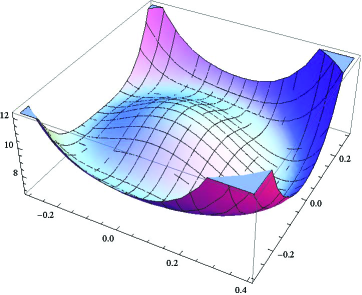
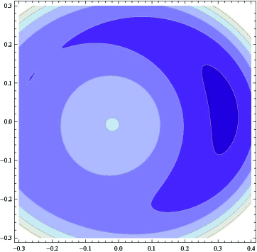
Figure 1: Graphs of $\Pi(x_{1},x_{2})$ and its contour for Example 1.

$$\Pi(x_{1},x_{2})=6\exp(2x_{1}^{2}+4.5x_{2}^{2})+4(8x_{1}^{2}+12.5x_{2}^{2}-1)^{2}-\frac{1}{2}(x_{1}^{2}+x_{2}^{2})-2x_{1}-x_{2}.$$

The corresponding canonical dual function is

$$\Pi^{d}(\varsigma_{1},\varsigma_{2})=-\frac{1}{2}(\frac{4}{4\varsigma_{1}+16\varsigma_{2}-1}+\frac{1}{9\varsigma_{1}+25\varsigma_{2}-1})-\varsigma_{1}(\ln(\varsigma_{1}/6)-1)-(\frac{1}{16}\varsigma_{2}^{2}+\varsigma_{2})$$

  

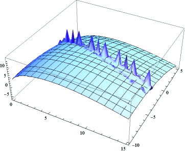
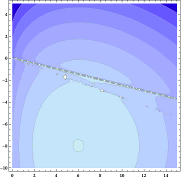
Figure 2: Graphs of $\Pi^{d}(\varsigma_{1},\varsigma_{2})$ and its contour for Example 1.

Its graph is shown by Figure 2. It is easy to find that the canonical dual problem $({\cal{P}}^{d})$ has three solutions:

$${\mbox{\boldmath$\varsigma$}}^{1}=[7.38697,-1.39206]^{T}\in{\cal S}_{a}^{+},$$

$${\mbox{\boldmath$\varsigma$}}^{2}=[6.00566,-7.97189]^{T}\in{\cal S}_{a}^{-},$$

$${\mbox{\boldmath$\varsigma$}}^{3}=[7.3106,-2.23695]^{T}\in{\cal S}_{a}^{-}.$$

By Theorem 1 we have three primal solutions:

$${\bf x}^{1}=[0.318731,0.0325932]^{T},$$

$${\bf x}^{2}=[-0.0191337,-0.00683777]^{T},$$

$${\bf x}^{3}=[-0.264945,0.112718]^{T}.$$

It is easily to check that

$$\Pi({\bf x}^{1})=\Pi^{d}({\mbox{\boldmath$\varsigma$}}^{1})=6.78671,$$

$$\Pi({\bf x}^{2})=\Pi^{d}({\mbox{\boldmath$\varsigma$}}^{2})=10.0225,$$

$$\Pi({\bf x}^{3})=\Pi^{d}({\mbox{\boldmath$\varsigma$}}^{3})=7.99906.$$

By Theorem 2 we know that ${\bf x}^{1}$ is a global minimizer of $\Pi({\bf x})$, ${\bf x}^{2}$ is a local maximizer of $\Pi({\bf x})$, and ${\bf x}^{3}=[-0.264945,0.112718]^{T}$ is a local minimizer of $\Pi({\bf x})$ (see Figure 1). By the fact that

$$x_{1}^{i} = F_{1}(x_{1}^{i},x_{2}^{i})=6\exp(2x_{1}^{i}+4.5x_{2}^{i})4x_{1}^{i}+8(8x_{1}^{i}+12.5x_{2}^{i}-1)16x_{1}^{i}-2,$$

$$x_{2}^{i} = F_{2}(x_{1}^{i},x_{2}^{i})=6\exp(2x_{1}^{i}+4.5x_{2}^{i})9x_{2}^{i}+8(8x_{1}^{i}+12.5x_{2}^{i}-1)25x_{2}^{i}-1,$$

hold for all $i=1,2,3$, we know that $\{{\bf x}^{i}\}$ ($i=1,2,3$) are all fixed points.

5 Application to Logarithmic and Quadratic Function

In this application, we let

$${W}(D{\bf x})=c_{1}\|D{\bf x}\|^{2}+c_{2}\|D{\bf x}\|^{2}\log\|D{\bf x}\|^{2}$$

where $D\in\mathbb{R}^{m\times n}$ is matrix, $c_{1}$, $c_{2}$ are real numbers. Clearly, ${W}(D{\bf x})$ is nonconvex and

$$F({\bf x})=\nabla P({\bf x})=2c_{1}(D^{T}D){\bf x}+2c_{2}((D^{T}D){\bf x})(\log\|D{\bf x}\|^{2}+1)$$

is non-monotone. The fixed point problem ${\bf x}=F({\bf x})$ can be reformulated as

$$({\cal{P}}):\;\;{\bar{{\bf x}}}=\arg{\rm sta}\left\{\Pi({\bf x})=c_{1}\|D{\bf x}\|^{2}+c_{2}\|D{\bf x}\|^{2}\log\|D{\bf x}\|^{2}-\frac{1}{2}\|{\bf x}\|^{2}-{\bf x}^{T}{\bf f}|\;\;{\bf x}\in{\mathbb{R}}^{n}\right\}.$$

By using the canonical measure

$$\xi={\Lambda}({\bf x})=\|D{\bf x}\|^{2}:\;{\mathbb{R}}^{n}\rightarrow{\cal E}_{a}={\mathbb{R}}^{+}=\{\xi\in{\mathbb{R}}|\;\xi\geq 0\},$$

the canonical function is $V(\xi)=c_{1}\xi+c_{2}\xi(\log\xi+1)$ and its Legendre conjugate is

$$V^{*}(\varsigma)=c_{2}\exp[\frac{1}{c_{2}}(\varsigma-c_{1})-1],$$

which is convex on its domain ${\cal E}^{*}_{a}={\mathbb{R}}$. In this case, we have the total complementary function

$$\Xi({\bf x},\varsigma)=\frac{1}{2}{\bf x}^{T}{\bf G}(\varsigma){\bf x}-{\bf x}^{T}{\bf f}-c_{2}\exp[\frac{1}{c_{2}}(\varsigma-c_{1})-1],$$

where ${\bf G}(\varsigma)=2\varsigma D^{T}D-{\bf I}$ and the canonical dual problem is

$$({\cal{P}}^{d}):\;\;\bar{\varsigma}=\arg{\rm sta}\left\{P^{d}(\varsigma)=-\frac{1}{2}{\bf f}^{T}{\bf G}^{-1}(\varsigma){\bf f}-c_{2}\exp[\frac{1}{c_{2}}(\varsigma-c_{1})-1]\;\;|\;\;\varsigma\neq 0\right\}.$$ (36)

Example 2

We first let $m=n=2$, $c_{1}=-8$, $c_{2}=10$, and

$$D=\left[\begin{array}[]{cc}3&0\\ 0&4\end{array}\right],\;\;{\bf f}=\left[\begin{array}[]{c}-5\\ 2\end{array}\right].$$

The primal function

  

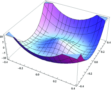
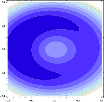
Figure 3: Graph of $\Pi(x_{1},x_{2})$ and its contour for Example 2.

$$\Pi(x_{1},x_{2})=-8(9x_{1}^{2}+16x_{2}^{2})+10(9x_{1}^{2}+16x_{2}^{2})\log(9x_{1}^{2}+16x_{2}^{2})-\frac{1}{2}(x_{1}^{2}+x_{2}^{2})-5x_{1}+2x_{2}$$

is nonconvex and its graph is shown in Figure 3. The corresponding canonical dual function is

$$\Pi^{d}(\varsigma)=-\frac{1}{2}(\frac{25}{18\varsigma-1}+\frac{4}{32\varsigma-1})-10\exp[0.1(\varsigma+8)-1]$$

For this example, the one dimensional canonical dual problem $({\cal{P}}^{d})$ can be solved easily (by using Mathematica) to obtain total three solutions (see Figure 4):

$$\varsigma^{1}=0.969642>\varsigma^{2}=-0.955077>\varsigma^{3}=-91.0174.$$

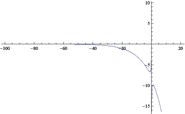
Figure 4: Graph of $\Pi^{d}(\varsigma)$ for Example 2.

Correspondingly, the three primal solutions are

$${\bf x}^{1}=\left[\begin{array}[]{c}-0.303886\\ 0.0666033\end{array}\right],\;\;{\bf x}^{2}=\left[\begin{array}[]{c}0.274855\\ -0.0633664\end{array}\right],\;\;{\bf x}^{3}=\left[\begin{array}[]{c}0.00305006\\ -0.000686446\end{array}\right].$$

It is easy to check that ${\bf x}^{i}=F({\bf x}^{i}),\;\;i=1,2,3$. Therefore, $\{{\bf x}^{i}\}$ are fixed points. Since $\varsigma^{1}\in{\cal S}^{+}_{a}=\{\varsigma\in{\mathbb{R}}|\;\varsigma>0\}$, we know that ${\bf x}^{1}$ is a globally stable fixed point. It is easy to check that ${\bf x}^{2}$ is a locally stable fixed point, ${\bf x}^{3}$ is a locally unstable fixed point, and

$$\Pi({\bf x}^{1})=\Pi^{d}(\varsigma^{1})=-9.84726,$$

$$\Pi({\bf x}^{2})=\Pi^{d}(\varsigma^{2})=-6.69103,$$

$$\Pi({\bf x}^{3})=\Pi^{d}(\varsigma^{3})=0.00739894.$$

Example 3

We now let $m=3$, $n=2$, $c_{1}=-15$, $c_{2}=9$, and

$$D=\left[\begin{array}[]{cc}0.3&0.2\\ 0.5&0.6\\ 0.4&0.7\end{array}\right],\;\;{\bf f}=\left[\begin{array}[]{c}1\\ 4\end{array}\right],$$

then the primal function is

  

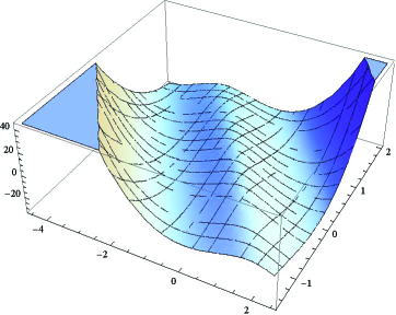
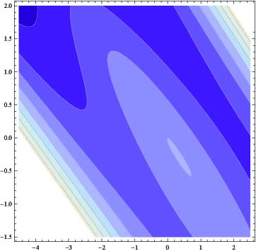
Figure 5: Graph of $\Pi({\bf x})$ and its contour for Example 3.

  

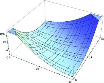
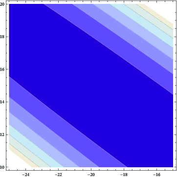
Figure 6: Graph of $\Pi({\bf x})$ and its contour for Example 3 around ${\bf x}^{1}$.

  

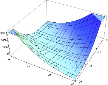
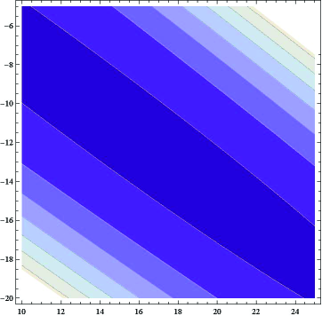
Figure 7: Graph of $\Pi({\bf x})$ and its contour for Example 3 around ${\bf x}^{2}$.

$$\Pi(x_{1},x_{2}) = 9(0.5x_{1}^{2}+1.28x_{1}x_{2}+0.89x_{2}^{2})\log(0.5x_{1}^{2}+1.28x_{1}x_{2}+0.89x_{2}^{2})$$

$$-15(0.5x_{1}^{2}+1.28x_{1}x_{2}+0.89x_{2}^{2})-\frac{1}{2}(x_{1}^{2}+x_{2}^{2})-x_{1}-4x_{2}.$$

Its graph is a nonconvex surface in ${\mathbb{R}}^{3}$, which has multiple critical points, but their locations can’t be find precisely as the surface is rather flat around these critical points (see Figure 5-7). However, its canonical dual is a single valued function

$$\Pi^{d}(\varsigma)=-\frac{1}{2}\left[\begin{array}[]{cc}1&4\end{array}\right]\left[\begin{array}[]{cc}\varsigma-1&1.28\varsigma\\ 1.28\varsigma&1.78\varsigma-1\end{array}\right]^{-1}\left[\begin{array}[]{c}1\\ 4\end{array}\right]-9\exp[\frac{1}{9}(\varsigma+15)-1]$$

and from its graph, we can see clearly that it has total five critical points (see Figure 8-9).

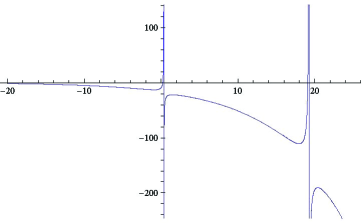
Figure 8: Graph of $\Pi^{d}(\varsigma)$ for Example 3.

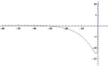
Figure 9: Graph of $\Pi^{d}(\varsigma)$ for Example 3 around $\varsigma^{2}$.

These critical points can be easily obtained by Mathematica:

$$\varsigma^{1}=20.396>\varsigma^{2}=17.9735>\varsigma^{3}=1.46219>\varsigma^{4}=-0.881733>\varsigma^{5}=-52.7144.$$

By Theorem 1, we have all the primal solutions:

$${\bf x}^{1}=\left[\begin{array}[]{c}-21.57\\ 16.065\end{array}\right],\;{\bf x}^{2}=\left[\begin{array}[]{c}18.937\\ -13.93\end{array}\right],\;{\bf x}^{3}=\left[\begin{array}[]{c}2.130\\ 0.008\end{array}\right],\;{\bf x}^{4}=\left[\begin{array}[]{c}0.546\\ -1.797\end{array}\right],\;{\bf x}^{5}=\left[\begin{array}[]{c}0.323\\ -0.272\end{array}\right].$$

Since $F({\bf x})$ is a potential operator, these stationary points are all fixed points of $F({\bf x})$. It is easy to find that the matrix ${\bf G}(\varsigma)$ has two singularity points: $\varsigma_{1}=19.266$ and $\varsigma_{2}=0.367$, therefore,

$${\cal S}^{+}_{a}=\{\varsigma\in{\mathbb{R}}|\;\;\varsigma>19.266\},\;\;{\cal S}^{-}_{a}=\{\varsigma\in{\mathbb{R}}|\;\;\varsigma<0.367\}.$$

By the facts that $\varsigma^{1}\in{\cal S}^{+}_{a}$ and $\varsigma^{5}\in{\cal S}^{-}_{a}$, we know that ${\bf x}^{1}$ is a globally stable fixed point, ${\bf x}^{5}$ is a locally unstable fixed point. Although $\varsigma^{4}\in{\cal S}^{-}_{a}$ is a local minimizer of $\Pi^{d}(\varsigma)$, we can’t say if ${\bf x}^{4}$ is a locally stable fixed point since $\dim{\cal X}_{a}=2\neq\dim{\cal S}_{a}=1.$ But by the complementary-dual principle and the order of the canonical dual solutions $\{\varsigma^{i}\}$ , we have

$$\Pi({\bf x}^{1})=\Pi^{d}(\varsigma^{1})=-190.381$$

$$< \Pi({\bf x}^{2})=\Pi^{d}(\varsigma^{2})=-110.759$$

$$< \Pi({\bf x}^{3})=\Pi^{d}(\varsigma^{3})=-21.7036$$

$$< \Pi({\bf x}^{4})=\Pi^{d}(\varsigma^{4})=-12.5735$$

$$< \Pi({\bf x}^{5})=\Pi^{d}(\varsigma^{5})=0.332915.$$

6 Conclusions

Based on the canonical duality theory, a unified model is proposed such that the general fixed point problems can be reformulated as a global optimization problem. This model is directly related to many other challenging problems in variational inequality, d.c. programming, chaotic dynamics, nonconvex analysis/PDEs, post-buckling of large deformed structures, phase transitions in solids, and computer science, etc (see [19] and references cited therein). By the complementary-dual principle, all the fixed points can be obtained analytically in terms of the canonical dual solutions. Their stability and extremality are identified by the triality theory. Applications are illustrated by problems governed by nonconvex polynomial, exponential and logarithmic functions. Our examples show that both globally stable and locally stable/unstable fixed point problems in ${\mathbb{R}}^{n}$ can be can be obtained easily by solving the associated canonical dual problems in ${\mathbb{R}}^{m}$ with $m<n$. However, the local stability condition for those fixed points ${\bar{{\bf x}}}(\bar{\mbox{\boldmath$\varsigma$}})$ with indefinite ${\bf G}(\bar{\mbox{\boldmath$\varsigma$}})$ still remains unknown and it deserves seriously study in the future. Also, the results presented in this paper can be generalized to problems with nonsmooth potential functions.

Acknowledgement: The research was supported by US Air Force Office of Scientific Research under the grants (AOARD) FA2386-16-1-4082 and FA9550-17-1-0151.

References

- [1] Ali, E. and Gao, D.Y. (2017). Improved Canonical Dual Finite Element Method and Algorithm for Post-Buckling Analysis of Nonlinear Gao Beam, Canonical Duality Theory: Unified Methodology for Multidisciplinary Study, D.Y. Gao, V. Latorre, and N. Ruan (eds). Springer, New York, 2017.
- [2] Bierlaire, M., Crittin, F.: Solving noisy, large-scale fixed-point problems and systems of nonlinear equations. Transportation Science, 40, 44–63 (2006)
- [3] Border, K.C.: Fixed Point Theorems with Applications to Economics and Game Theory. Cambridge University Press, New York (1985)
- [4] Chen, Y. and Gao, D.Y. (2016). Global solutions to nonconvex optimization of 4th-order polynomial and log-sum-exp functions. Journal of Global Optimization,64 (3): 417-431.
- [5] Ciarlet, P.G. (2013). Linear and Nonlinear Functional Analysis with Applications, SIAM, Philadelphia.
- [6] Eaves, B.C. (1972). Homotopies for computation of fixed points. Math. Programming, 3, 1–12
- [7] Ekeland, I. and Temam, R. (1976). Convex Analysis and Variational Problems, North-Holland.
- [8] Gao, D.Y. (1996). Nonlinear elastic beam theory with applications in contact problem and variational approaches, Mech. Research Commun., 23 (1), 11-17.
- [9] Gao, D.Y. (2000). Duality Principles in Nonconvex Systems: Theory, Methods and Applications. Springer, New York.
- [10] Gao, D.Y.(2000). Finite deformation beam models and triality theory in dynamical post-buckling analysis, Int. J. Non-Linear Mechanics, 5, 103-131.
- [11] Gao, D.Y. (2000). Canonical dual transformation method and generalized triality theory in nonsmooth global optimization, J. Global Optimization, 17 (1/4): 127-160.
- [12] Gao,D.Y.(2005). Sufficient conditions and perfect duality in nonconvex minimization with inequality constraints. Journal of Industrial and Management Optimization, 1(1): 59-69.
- [13] Gao,D.Y.(2006). Complete solutions and extremality criteria to polynomial optimization problems. Journal of Global Optimization, 35: 131-143.
- [14] Gao,D.Y.(2007). Solutions and optimality to box constrained nonconvex minimization problems. Journal of Industrial and Management Optimization, 3(2): 293-304.
- [15] Gao, D.Y. (1999). General Analytic Solutions and Complementary Variational Principles for Large Deformation Nonsmooth Mechanics. Meccanica 34, 169-198.
- [16] Gao, D.Y. (1999). Pure complementary energy principle and triality theory in finite elasticity, Mech. Res. Comm. 26 (1), 31-37.
- [17] Gao, D.Y. , On unified modeling, theory, and method for solving multi-scale global optimization problems, Numerical Computations: Theory And Algorithms,, (Editors) Y. D. Sergeyev, D. E. Kvasov and M. S. Mukhametzhanov, AIP Conference Proceedings 1776, 020005, 2016.
- [18] Gao, D.Y. (2016). On unified modeling, canonical duality-triality theory, challenges and breakthrough in optimization, https://arxiv.org/abs/1605.05534.
- [19] Gao, D.Y.,Latorre,V., and Ruan,N. (2017). Canonical Duality Theory: Unified Methodology for Multidisciplinary Study, Springer, New York, 377pp.
- [20] Gao,D.Y., Ruan,N.(2010). Solutions to quadratic minimization problems with box and integer constraints. Journal of Global Optimization, 47(3): 463-484.
- [21] Gao, D.Y. , Ruan, N. and Latorre, V. (2017). Canonical duality-triality theory: Bridge between nonconvex analysis/mechanics and global optimization in complex systems. In Canonical Duality Theory: Unified Methodology for Multidisciplinary Study, D.Y. Gao, V. Latorre, and N. Ruan (eds). Springer, New York, 1-48.
- [22] Gao, D.Y., Ruan, N., Sherali, H. (2009). Solutions and optimality criteria for nonconvex constrained global optimization problems with connections between canonical and Lagrangian duality. J. Glob. Optim. 45, 473-497.
- [23] Gao, D.Y., Ruan,N., Sherali, H.D.(2010). Canonical duality solutions for fixed cost quadratic program. Optimization and Optimal Control, 139-156.
- [24] Gao, D.Y., Ruan, N., Sherali, H.D.: Solutions and optimality criteria for nonconvex constrained global optimization problems. Journal of Global Optimization, 45, 473–497 (2009)
- [25] Gao, D.Y. and Strang ,G.(1989). Geometric nonlinearity: Potential energy, complementary energy, and the gap function.Quarterly Journal of Applied Mathematics, XLVII(3): 487-504.
- [26] Gao, D.Y. and Wu, C. (2017). Triality theory for general unconstrained global optimizationproblems. In Canonical Duality Theory: Unified Methodology for Multidisciplinary Study, D.Y. Gao, V. Latorre, and N. Ruan (eds). Springer, New York, 127-154.
- [27] Gao, D.Y., Yu, H.F. (2008). Multi-scale modelling and canonical dual finite element method in phase transitions of solids. Int. J. Solids Struct., 45: 3660-3673.
- [28] Hirsch, M.D., Papadimitriou, C., Vavasis, S.: Exponential lower bounds for finding Brouwer fixed points. Journal of Complexity, 5, 379–416 (1989)
- [29] Holzapfel, G.A. (2000). Nonlinear Solid Mechanics: A Continuum Approach for Engineering. Wiley. ISBN 978-0471823193.
- [30] Huang, Z., Khachiyan, L., Sikorski, K.: Approximating fixed points of weakly contracting mappings. J. Complexity, textbf15, 200–213 (1999)
- [31] Jin, Z. and Gao, D.Y. (2017). On modeling and global solutions for d.c. optimization problems by canonical duality theory, Appl. Math. Comp., 296:168–181.
- [32] Latorre, V. and Gao, D.Y. (2016). Canonical duality for solving general nonconvex constrained problems, Optimization Letters.
- [33] Latorre, V. and Gao, D.Y. (2016). Global optimal trajectory in chaos and NP-hardness, Int. J. Bifurcation Chaos 26:1650142.
- [34] Liu, G.S. , Gao, D.Y. and Wang, S.Y. (2017). Canonical duality theory for solving non-monotone variational inequality problems, in Canonical Duality Theory: Unified Methodology for Multidisciplinary Study, D.Y. Gao, V. Latorre, and N. Ruan (eds). Springer, New York, 155-172.
- [35] Marsden, J.E. and Hughes, T.J.R.(1983). Mathematical Foundations of Elasticity, Prentice-Hall, 1983.
- [36] Ruan, N. and Gao, D.Y. (2014). Canonical duality approach for nonlinear dynamical systems, IMA J. Appl. Math., 79: 313-325.
- [37] Scarf, H.: The approximation of fixed point of a continuous mapping. SIAM J. Appl. Math, 35, 1328–1343 (1967)
- [38] Scarf, H. E., Hansen, T.: Computation of Economic Equibibria. Yale University Press (1973)
- [39] Shellman, S., Sikorski, K.: A two-dimensional bisection envelope algorithm for fixed points. J. Complexity, 2, 641–659 (2002)
- [40] Shellman, S., Sikorski, K.: A recursive algorithm for the infinity-norm fixed point problem. J. Complexity, 19, 799–834 (2003)
- [41] Smart, D.R.: Fixed Point Theorems. Cambridge University Press, Cambridge (1980)
- [42] Wang Z.B., Fang, S.-C., Gao, D.Y., Xing W.X.(2008). Global extremal conditions for multi-integer quadratic programming. Journal of Industrial and Management Optimization, 4(2): 213-225.
- [43] Yang, Z.: Computing Equilibria and Fixed Points: The Solution of Nonlinear Inequalities. Kluwer Academic Publishers, Dordrecht (1999)