Perfect transmission at oblique incidence by trigonal warping in graphene P-N junctions

Abstract

We develop an analytical mode-matching technique for the tight-binding model to describe electron transport across graphene P-N junctions. This method shares the simplicity of the conventional mode-matching technique for the low-energy continuum model and the accuracy of the tight-binding model over a wide range of energies. It further reveals an interesting phenomenon on a sharp P-N junction: the disappearance of the well-known Klein tunneling (i.e., perfect transmission) at normal incidence and the appearance of perfect transmission at oblique incidence due to trigonal warping at energies beyond the linear Dirac regime. We show that this phenomenon arises from the conservation of a generalized pseudospin in the tight-binding model. We expect this effect to be experimentally observable in graphene and other Dirac fermions systems, such as the surface of three-dimensional topological insulators.

I Introduction

Klein tunneling Klein (1929), the unimpeded penetration of relativistic particles regardless of the height and width of potential barriers, is an exotic effect compared with the exponential-decaying transmission of nonrelativistic particles Allain and Fuchs (2011). In 2006, the seminal theoretical work of Katsnelson et al. Katsnelson et al. (2006) brought about the possibility of demonstrating Klein tunneling across electrostatic junctions in graphene. This proposal has stimulated widespread theoretical Cheianov and Fal’ko (2006); Pereira et al. (2006); Bai and Zhang (2007); Beenakker et al. (2008); Setare and Jahani (2010); Roslyak et al. (2010); Zeb et al. (2008); Sonin (2009); Schelter et al. (2010); Yang et al. (2011); Rozhkov et al. (2011); Liu et al. (2012); Giavaras and Nori (2012); Rodriguez-Vargas et al. (2012); Popovici et al. (2012); Heinisch et al. (2013); Logemann et al. (2015); Oh et al. (2016); Erementchouk et al. (2016); Downing and Portnoi (2017) and experimental Huard et al. (2007); Gorbachev et al. (2008); Stander et al. (2009); Young and Kim (2009); Rossi et al. (2010); Sajjad et al. (2012); Sutar et al. (2012); Rahman et al. (2015); Guti rrez et al. (2016); Chen et al. (2016); Laitinen et al. (2016); Bai et al. (2017) interest and shed light on possible electronic applications Sajjad and Ghosh (2011); Jang et al. (2013); Wilmart et al. (2014); Chen and Chang (2015); de Sousa et al. (2017); Tan et al. (2017).

Graphene is a 2D layer of carbon atoms on a honeycomb lattice [Fig. 1(a)]. The conduction band and the valence band touch each other at six Dirac points, but only two of them are inequivalent, as denoted by $\mathbf{K}$ and $\mathbf{K}^{\prime}$ in the right panel of Fig. 1(a). According to group theory Bir and Pikus (1974), the D_6h point group symmetry of the honeycomb lattice determines the global hexagonal symmetry of the graphene energy band over the first Brillouin zone, while the local D_3h symmetry of each valley determines the local triangular symmetry of the energy band in this valley. Close to the Dirac point, say $\mathbf{K}$, the energy dispersion as a function of the reduced wave vector $\mathbf{q}\equiv\mathbf{k}-\mathbf{K}$ is linear and isotropic. Away from the Dirac point, however, the D_3h local symmetry becomes important and the constant energy contour approaches a regular triangle with a side length $2\pi/3$ [see Fig. 1(b)]. This is commonly referred to as trigonal warping, which increases rapidly with energy [Fig. 1(c)]. Note that throughout this work we use the carbon-carbon bond length $a=0.142$ nm as the unit of length and the nearest-neighbor hopping energy $t_{0}=2.7$ eV as the unit of energy Castro Neto et al. (2009).

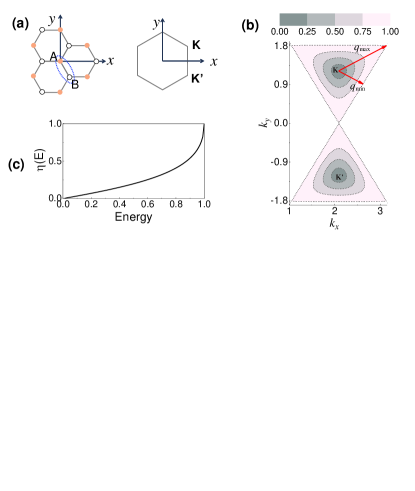
Figure 1: (a) Honeycomb lattice of graphene in the real space (left, the dashed ellipse for a unit cell) and reciprocal space (right). (b) Constant energy contour in the two inequivalent valleys: $\mathbf{K}$ and $\mathbf{K}^{\prime}$. (c) Degree of trigonal warping $\eta(E)\equiv[q_{\max}(E)-q_{\min}(E)]/q_{\min}(E)$ as a function of energy $E$, where $q_{\mathrm{max}}(E)$ [$q_{\mathrm{min}}(E)$] is the largest (smallest) reduced wave vector on the constant energy contour $E$ [see panel (b)].

Trigonal warping is a well-known feature of the graphene energy band beyond the linear regime Castro Neto et al. (2009) and its influence on the electron transport is receiving growing interest, including the observation of broken chirality by trigonal warping in transport measurements Wu et al. (2007); Dombrowski et al. (2017), the influence Xing et al. (2010); Reijnders and Katsnelson (2017) of trigonal warping on the famous Veselago focusing across graphene P-N junctions Cheianov et al. (2007); Lee et al. (2015); Chen et al. (2016), and potential applications of trigonal warping for producing valley-polarized electrons in N-P-N junction Garcia-Pomar et al. (2008), double barriers Jr et al. (2009), and other junctions Logemann et al. (2015). To incorporate trigonal warping, the simplest method Garcia-Pomar et al. (2008); Jr et al. (2009) is to introduce nonlinear corrections to the widely used low-energy linear continuum model. The nearest-neighbor tight-binding model captures the hexagonal lattice symmetry and hence is commonly used Castro Neto et al. (2009); Xing et al. (2010); Logemann et al. (2015); Reijnders and Katsnelson (2017) to study the trigonal warping effect over a wide energy range. At energies below 1 eV, this model gives very accurate energy bands, but its deviation from the ab initio calculation becomes significant at energies approaching the Van Hove singularity at $\sim 3$ eV Reich et al. (2002). However, transport calculations in the tight-binding model are usually based on the recursive Green’s function method Datta (1995); Ferry and Goodnick (1997); Lewenkopf and Mucciolo (2013); Zhang et al. (2017) and hence are numerical. Moreover, previous studies on Klein tunneling mainly focus on the low-energy linear regime of graphene, leaving the effect of trigonal warping largely unexplored. In particular, it is well known that the Klein tunneling (i.e., perfect transmission) at normal incidence originates from the conservation of the pseudospin Katsnelson et al. (2006); Beenakker (2008). However, this simple physical picture is based on the linear continuum model and hence is limited to the low-energy linear Dirac regime. It is not clear whether a similar physical picture exists in the tight-binding model and over a wide range of energies.

In this paper, we develop an analytical mode-matching technique in the tight-binding model for electron transport across graphene P-N junctions. The key is to introduce a titled coordinate system, reduce the 2D junction into a 1D chain, and then perform mode-matching at the P-N interface, in a similar way to the mode matching in the continuum model Ferry and Goodnick (1997); Katsnelson et al. (2006). As a result, this method shares the simplicity of the mode-matching method in the low-energy continuum model and the accuracy of the tight-binding model over a wide range of energies. To focus on trigonal warping, we consider the electron transmission across a sharp P-N interface along the zigzag direction in the energy range $E\in[-1,+1]$, where the intervalley scattering is absent Garcia-Pomar et al. (2008); but trigonal warping is significant and can be described reasonably by the tight-binding model. The results show that beyond the linear regime, the Klein tunneling at normal incidence becomes imperfect; i.e., finite backscattering occurs. Interestingly, we find that perfect transmission is still possible, but the critical incident angle for perfect transmission deviates from zero, and the deviation increases with increasing trigonal warping. We introduce the concept of a generalized pseudospin in the tight-binding model and show that its conservation across the P-N interface is responsible for the perfect transmission at oblique incidence. This generalizes the well-known pseudospin picture for perfect transmission, previously limited to the linear Dirac regime, to a wide energy range $E\in[-1,+1]$. The continuum model with a second-order nonlinear correction fails to describe this phenomenon quantitatively. We expect this phenomenon to be experimentally observable.

The rest of this paper is organized as follows. In Sec. II, we introduce the tilted coordinates, present the analytical mode-matching method, and introduce the generalized pseudospin picture for perfect transmission. In Sec. III, we discuss the perfect transmission at oblique incidence and the failure of the continuum model. Finally, we give a brief conclusion in Sec. IV.

II Mode-matching technique in tilted coordinates

Figure 2: (a) Graphene junction with a zigzag interface. The inset sketches the Dirac points of the left region and the right region. (b) One-dimensional chain along the $X$ axis, with two orbitals $A$ and $B$ in one unit cell.

For specificity, we consider a graphene P-N junction with a sharp, zigzag interface separating the left region and the right region [Fig. 2(a)], leaving the more general cases to the end of this section. The tight-binding Hamiltonian of the junction is the sum of the (nearest-neighbor) tight-binding Hamiltonian for uniform graphene Castro Neto et al. (2009) and the on-site junction potential, which takes a constant value $V_{\mathrm{L}}$ ($V_{\mathrm{R}}$) for all the carbon sites in the left (right) region [see the inset of Fig. 2(a)]. The Fermi level $E_{F}$, which can be tuned by electric gating, determines the doping level in the left (right) region as $\varepsilon_{\mathrm{L}}\equiv E_{F}-V_{\mathrm{L}}$ ($\varepsilon_{\mathrm{R}}\equiv E_{F}-V_{\mathrm{R}}$), where a positive (negative) doping level means electron or N (hole or P) doping. Here we consider a P-N junction with $\varepsilon_{\mathrm{L}}>0$ and $\varepsilon_{\mathrm{R}}<0$; i.e., the left region is N doped and the right region is P doped.

In addition to the ortho-normalized basis vectors $(\mathbf{e}_{x},\mathbf{e}_{y})$ of the conventional Cartesian coordinate system, we introduce a tilted coordinate system characterized by the nonorthogonal basis vectors $(\mathbf{e}_{X},\mathbf{e}_{Y})$ [see Fig. 2(b)]. The tilted vectors $\mathbf{e}_{X}$ and $\mathbf{e}_{Y}$ are actually the two primitive vectors for the Bravais lattice of uniform graphene and are connected to $(\mathbf{e}_{x},\mathbf{e}_{y})$ by

$$\left\{\begin{array}[c]{l}\mathbf{e}_{X}=\sqrt{3}(\dfrac{\sqrt{3}}{2}\mathbf{e}_{x}-\dfrac{1}{2}\mathbf{e}_{y}),\\ \mathbf{e}_{Y}=\sqrt{3}\mathbf{e}_{y},\end{array}\right.\Leftrightarrow\left\{\begin{array}[c]{l}\mathbf{e}_{x}=\dfrac{2\mathbf{e}_{X}+\mathbf{e}_{Y}}{3},\\ \mathbf{e}_{y}=\dfrac{\mathbf{e}_{Y}}{\sqrt{3}}.\end{array}\right.$$

The Cartesian components $k_{x}\equiv\mathbf{k}\cdot\mathbf{e}_{x}$ and $k_{y}\equiv\mathbf{k}\cdot\mathbf{e}_{y}$ of a wave vector $\mathbf{k}$ in the reciprocal space are connected to the tilted components $k_{X}\equiv\mathbf{k}\cdot\mathbf{e}_{X}$ and $k_{Y}\equiv\mathbf{k}\cdot\mathbf{e}_{Y}$ via

$$\left\{\begin{array}[c]{l}k_{X}=\sqrt{3}(\dfrac{\sqrt{3}}{2}k_{x}-\dfrac{1}{2}k_{y}),\\ k_{Y}=\sqrt{3}k_{y},\end{array}\right.\Leftrightarrow\left\{\begin{array}[c]{l}k_{x}=\dfrac{2k_{X}+k_{Y}}{3},\\ k_{y}=\dfrac{k_{Y}}{\sqrt{3}}.\end{array}\right.$$ (1)

For a position vector $\mathbf{R}$ in the real space, we define the tilted components $R_{X},R_{Y}$ through the expansion

$$\mathbf{R}\equiv R_{X}\mathbf{e}_{X}+R_{Y}\mathbf{e}_{Y}\Rightarrow\left\{\begin{array}[c]{l}R_{X}=\dfrac{2R_{x}}{3},\\ R_{Y}=\dfrac{R_{x}+\sqrt{3}R_{y}}{3}.\end{array}\right.$$

These definitions lead to the convenient expression $\mathbf{k}\cdot\mathbf{R}=k_{x}R_{x}+k_{y}R_{y}=k_{X}R_{X}+k_{Y}R_{Y}$, although $\mathbf{k}\neq k_{X}\mathbf{e}_{X}+k_{Y}\mathbf{e}_{Y}$ and $R_{X,Y}\neq\mathbf{R}\cdot\mathbf{e}_{X,Y}$ since $(\mathbf{e}_{X},\mathbf{e}_{Y})$ are not ortho-normalized. An arbitrary vector $\mathbf{O}$ can be denoted by $\mathbf{O}=(O_{x},O_{y})=(O_{X},O_{Y})_{\mathrm{T}}$.

II.1 Tight-binding model for uniform graphene

Here we consider uniform graphene with $\varepsilon_{\mathrm{L}}=\varepsilon_{\mathrm{R}}=E_{F}$ to illustrate the usage of the tilted coordinates and establish the relevant notations and some important concepts.

As shown in Fig. 1(a) or 2(a), the honeycomb lattice of graphene consists of two sublattices (denoted by $A$ and $B$) and each unit cell contains two carbon atoms, one on each sublattice. The unit cell $(m,n)$ locates at $\mathbf{R}_{m,n}=m\mathbf{e}_{X}+n\mathbf{e}_{Y}=(m,n)_{\mathrm{T}}$, and the relative displacements of the two carbon atoms inside this unit cell are $\boldsymbol{\tau}_{A}=0$ and $\boldsymbol{\tau}_{B}=(1/2,-\sqrt{3}/2)$. The tight-binding Hamiltonian of uniform graphene is

$$\hat{H}_{0}=-\sum_{m,n}(|m+1,n,A\rangle+|m,n-1,A\rangle+|m,n,A\rangle)\langle m,n,B|-h.c.,$$

where $|m,n,\lambda\rangle$ ($\lambda=A,B$) denotes the carbon atom on the sublattice $\lambda$. To utilize the translational invariance of graphene with the primitive vector $\mathbf{e}_{Y}$ along the $Y$ axis, we make a Fourier transform from the on-site basis $\{|m,n,\lambda\rangle\}$ to the hybrid basis (i.e., on-site basis along the $X$ axis and Bloch basis along the $Y$ axis)

$$|m,k_{Y},\lambda\rangle=\frac{1}{\sqrt{N_{Y}}}\sum_{n}e^{i{n}k_{Y}}|m,n,\lambda\rangle,$$ (2)

where $N_{Y}$ is the normalization length along the $Y$ axis and $k_{Y}\in[0,2\pi]$. Under this basis $\hat{H}_{0}=\sum_{k_{Y}}\hat{h}(k_{Y})$, where

$$\hat{h}(k_{Y})=-\sum_{m}[(1+e^{ik_{Y}})|m,k_{Y},A\rangle+|m+1,k_{Y},A\rangle]\langle m,k_{Y},B|-h.c..$$

For a given $k_{Y}$, the Hamiltonian $\hat{h}(k_{Y})$ describes a 1D chain along the $X$ axis [see Fig. 2(b)], with two orbitals $A$ and $B$ in each unit cell. The 2$\times$2 on-site energy of each unit cell is

$$\mathbf{h}(k_{Y})=-\left[\begin{array}[c]{cc}0&1+e^{ik_{Y}}\\ 1+e^{-ik_{Y}}&0\end{array}\right]$$ (3)

and the 2$\times$2 hopping matrix from unit cell $m+1$ to $m$ is

$$\mathbf{t}\equiv\langle m|\hat{h}(k_{Y})|m+1\rangle=\begin{bmatrix}0&0\\ -1&0\end{bmatrix}.$$ (4)

So the Fourier transform reduces the 2D graphene into decoupled 1D chains [Fig. 2(b)] parametrized by different $k_{Y}$’s.

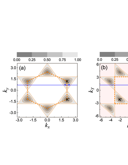
Figure 3: Fermi contours $E_{F}=0.25$, $0.5$, $0.75$, and $1.0$ for the conduction band of uniform graphene in Cartesian (a) and tilted (b) coordinate system. The dashed orange lines mark the first Brillouin zone. The horizontal blue line corresponds to $k_{y}=0.70$ in (a) and $k_{Y}=\sqrt{3}k_{y}=1.21$ in (b).

Next, to utilize the translational invariance along the $X$ axis with the primitive vector $\mathbf{e}_{X}$, we make another Fourier transform along $X$ to get the full Bloch basis:

$$|\mathbf{k},\lambda\rangle\equiv\frac{1}{\sqrt{N_{X}}}\sum_{m}e^{i{m}k_{X}}|m,k_{Y},\lambda\rangle=\frac{1}{\sqrt{N}}\sum_{m,n}e^{i\mathbf{R}_{m,n}\cdot\mathbf{k}}|m,n,\lambda\rangle$$

parameterized by the wave vector $\mathbf{k}=(k_{X},k_{Y})_{\mathrm{T}}$. This transformation further decouples the lattice degree of freedom along the $X$ axis and leads to

$$\hat{H}_{0}=\sum_{\mathbf{k}}[|\mathbf{k},A\rangle,|\mathbf{k},B\rangle]\mathbf{H}_{0}(\mathbf{k})\begin{bmatrix}\langle\mathbf{k},A|\\ \langle\mathbf{k},B|\end{bmatrix},$$

where

$$\mathbf{H}_{0}(\mathbf{k})\equiv\begin{bmatrix}0&f(\mathbf{k})\\ f(-\mathbf{k})&0\end{bmatrix}$$ (5)

is the 2$\times$2 tight-binding Hamiltonian and

$$f(\mathbf{k})=-(1+e^{ik_{Y}}+e^{-ik_{X}}).$$ (6)

The eigenenergies are $E^{(\pm)}(\mathbf{k})=\pm|f(\mathbf{k})|$, where

$$\left|f(\mathbf{k})\right| =\sqrt{3+2[\cos k_{X}+\cos k_{Y}+\cos(k_{X}+k_{Y})]}$$

$$=\sqrt{3+2\cos(\sqrt{3}k_{y})+4\cos\frac{3k_{x}}{2}\cos\frac{\sqrt{3}k_{y}}{2}}.$$ (7)

The corresponding eigenstates are $|\Phi^{(\pm)}(\mathbf{k})\rangle=[1,\pm f^{\ast}(\mathbf{k})/\left|f(\mathbf{k})\right|]^{T}$. Note that we normalize every spinor to $\sqrt{2}$ throughout this work.

In the Cartesian coordinates, the first Brillouin zone is a regular hexagon, as shown in Fig. 3(a). In the tilted coordinates, the first Brillouin zone is a square $k_{X},k_{Y}\in[-\pi,\pi]$, as shown in Fig. 3(b). The two inequivalent Dirac points are

$$\mathbf{K} \equiv\left(\frac{2\pi}{3},\frac{2\pi}{3\sqrt{3}}\right)=\left(\frac{2\pi}{3},\frac{2\pi}{3}\right)_{\mathrm{T}},$$

$$\mathbf{K}^{\prime} \equiv\left(\frac{2\pi}{3},-\frac{2\pi}{3\sqrt{3}}\right)=\left(\frac{4\pi}{3},-\frac{2\pi}{3}\right)_{\mathrm{T}}\longrightarrow\left(-\frac{2\pi}{3},-\frac{2\pi}{3}\right)_{\mathrm{T}},$$

where in the last step of the second line we have shifted $\mathbf{K}^{\prime}$ by a reciprocal vector along the $X$ axis.

The continuum model Hamiltonian is obtained from $\mathbf{H}_{0}(\mathbf{k})$ by considering $\mathbf{k}$ in a given valley, say $\mathbf{K}$, defining the reduced wave vector $\mathbf{q}\equiv\mathbf{k}-\mathbf{K}$, and expanding $f(\mathbf{k})$ into Taylor series with respect to $\mathbf{q}$. For example, expanding $f(\mathbf{k})$ up to the first order of $\mathbf{q}$ gives the widely used linear continuum model. For the $\mathbf{K}$ valley, we have $f(\mathbf{k})\approx v_{F}|\mathbf{q}|e^{-i(\pi/6-\theta_{\mathbf{q}})}$ and hence the linear continuum model

$$\mathbf{H}_{\mathbf{K}}(\mathbf{q})=v_{F}|\mathbf{q}|\begin{bmatrix}0&e^{-i(\pi/6-\theta_{\mathbf{q}})}\\ e^{i(\pi/6-\theta_{\mathbf{q}})}&0\end{bmatrix},$$ (8)

where $v_{F}\equiv 3/2$ is the Fermi velocity and $\theta_{\mathbf{q}}$ is the azimuth angle of $\mathbf{q}$ in the Cartesian coordinates. For the $\mathbf{K}^{\prime}$ valley, $f(\mathbf{k})\approx-v_{F}|\mathbf{q}|e^{i(\pi/6-\theta_{\mathbf{q}})}$; thus

$$\mathbf{H}_{\mathbf{K}^{\prime}}(\mathbf{q})=-v_{F}|\mathbf{q}|\begin{bmatrix}0&e^{i(\pi/6-\theta_{\mathbf{q}})}\\ e^{-i(\pi/6-\theta_{\mathbf{q}})}&0\end{bmatrix}.$$ (9)

The linear continuum model for either valley gives the same isotropic, linear dispersion $E^{(\pm)}(\mathbf{q})=\pm v_{F}|\mathbf{q}|$ that totally ignores the trigonal warping. The corresponding eigenstates are $|\Phi_{\mathbf{K}}^{(\pm)}(\mathbf{q})\rangle=[1,\pm e^{i(\pi/6-\theta_{\mathbf{q}})}]^{T}$ for the $\mathbf{K}$ valley and $|\Phi_{\mathbf{K}^{\prime}}^{(\pm)}(\mathbf{q})\rangle=[1,\mp e^{-i(\pi/6-\theta_{\mathbf{q}})}]^{T}$ for the $\mathbf{K}^{\prime}$ valley. By expanding $f(\mathbf{k})$ into high orders of $\mathbf{q}$, trigonal warping can be included into the continuum model.

Now we discuss a distinguishing feature of the tight-binding model compared with all the continuum models (including those with high-order corrections for trigonal warping): the existence of “abnormal” evanescent states. Let us consider a given $k_{y}$ (or $q_{y}$) and determine the $k_{x}$ (or $q_{x}$) of all the eigenstates on the Fermi level. For $q_{y}<q_{F}\equiv|E_{F}|/v_{F}$, the linear continuum model of either valley gives two traveling eigenstates characterized by the reduced wave vector$\ (\pm(q_{F}^{2}-q_{y}^{2})^{1/2},q_{y})$ in the Cartesian coordinate. For the tight-binding model, $k_{x}$ is determined by $E_{F}=\mathrm{sgn}(E_{F})|f(\mathbf{k})|$, where $\mathbf{k}\equiv(k_{x},k_{y})$ and $\mathrm{sgn}(x)\equiv+1$ for $x>0$ and $-1$ for $x<0$. The solutions can be visualized as the two intersection points between the horizontal line $k_{y}$ and the Fermi contour $E_{F}=\mathrm{sgn}(E_{F})|f(\mathbf{k})|$ in the $(k_{x},k_{y})$ plane; e.g., for $E_{F}=0.75$ and $k_{y}=0.70$, we obtain two traveling eigenstates [blue dots in Fig. 3(a)]. When $k_{y}$ approaches the Dirac point, the eigenstates from the tight-binding model approach those from the linear continuum model. Similarly, in the tilted coordinate system, the eigenstates with a given $k_{Y}$ on the Fermi level can also be determined as the two intersection points between the horizontal line $k_{Y}$ and the Fermi contour $E_{F}=\mathrm{sgn}(E_{F})|f(\mathbf{k})|$ in the $(k_{X},k_{Y})_{\mathrm{T}}$ plane, as shown in Fig. 3(b) for $E_{F}=0.75$ and $k_{Y}=1.21$.

Surprisingly, in addition to these two “normal” eigenstates, the tight-binding model also has two extra, “abnormal” eigenstates. To make this clear, we follow Ref. Zhang et al., 2017 and solve the 1D Schrödinger equation

$$-\mathbf{t}^{{\dagger}}|\Phi(m-1)\rangle+(E-\mathbf{h}(k_{Y})\mathbf{)}|\Phi(m)\rangle-\mathbf{t}|\Phi(m+1)\rangle=0$$ (10)

for the 1D chain along the $X$ axis under the Bloch condition $|\Phi(m)\rangle=e^{imk_{X}}|\Phi\rangle$, where $k_{X}$ may be either real or complex. Equation (10) can be written as

$$\mathbf{H}_{0}(\mathbf{k})|\Phi\rangle=E|\Phi\rangle,$$ (11)

where $\mathbf{k}\equiv(k_{X},k_{Y})_{\mathrm{T}}=(k_{x},k_{y})$ is the wave vector and $\mathbf{H}_{0}(\mathbf{k})$ is the 2$\times$2 Hamiltonian of the tight-binding model [see Eq. (5)]. For a given, real wave vector $\mathbf{k}$, Eq. (11) reproduces the energy dispersions and eigenstates of uniform graphene. Here we need to find all the eigenstates with a given $k_{Y}$ on the Fermi level. For this purpose, we let $\lambda\equiv e^{ik_{X}}$ be the propagation phase along the $+X$ axis by one unit cell, set $E=E_{F}$, and rewrite Eq. (10) as

$$[-\mathbf{t}^{\dagger}+\lambda(E_{F}-\mathbf{h}(k_{Y})\mathbf{)}-\lambda^{2}\mathbf{t}]|\Phi\rangle=0,$$ (12)

from which we obtain four solutions for $\lambda$ (and hence $k_{X}$) and $|\Phi\rangle$. Two solutions correspond to the “normal” eigenstates and can be explicitly obtained by rewriting Eq. (12) as an explicit quadratic equation for $\lambda$:

$$(1+e^{ik_{Y}})\lambda^{2}+[(3+2\cos k_{Y})-E_{F}^{2}]\lambda+(1+e^{-ik_{Y}})=0.$$

The other two solutions are “abnormal” evanescent eigenstates, including a right-going one

$$\lambda_{0}=0,\ \ \ |\Phi_{0}\rangle=\begin{bmatrix}\sqrt{2}\\ 0\end{bmatrix}$$ (13)

and a left-going one

$$\lambda_{\infty}=\infty,\ \ |\Phi_{\infty}\rangle=\begin{bmatrix}0\\ \sqrt{2}\end{bmatrix}.$$ (14)

Finally we discuss the physical meaning of these “abnormal” evanescent eigenstates. The wave function of the right-going one [Eq. (13)] starting from a unit cell $m_{0}$ is defined in the half plane on the right of $m_{0}$ only (i.e., $m\geq m_{0}$):

$$|\Phi_{0}(m|m_{0})\rangle=\lambda_{0}^{m-m_{0}}|\Phi_{0}\rangle=\left\{\begin{array}[c]{ll}|\Phi_{0}\rangle&(m=m_{0}),\\ 0&(m\geq m_{0}+1).\end{array}\right.$$

The wave function of the left-going one [Eq. (14] starting from a unit cell $m_{0}$ is defined in the half plane on the left of $m_{0}$ only (i.e., for $m\leq m_{0}$):

$$|\Phi_{\infty}(m|m_{0})\rangle=\lambda_{\infty}^{m-m_{0}}|\Phi_{\infty}\rangle=\left\{\begin{array}[c]{ll}|\Phi_{\infty}\rangle&(m=m_{0}),\\ 0&(m\leq m_{0}-1).\end{array}\right.$$

Using $\mathbf{t}^{\dagger}|\Phi_{0}\rangle=\mathbf{t}|\Phi_{\infty}\rangle=0$, we can readily verify that $|\Phi_{0}(m|m_{0})\rangle$ ($|\Phi_{\infty}(m|m_{0})\rangle$) indeed satisfies the Schrödinger equation Eq. (10) with $m\geq m_{0}+1$ ($m\leq m_{0}-1$), so it is indeed an eigenstate on the Fermi level of uniform graphene, although it only exists in the half plane $m\geq m_{0}$ ($m\leq m_{0}$). These “abnormal” evanescent eigenstates originate from the singularity of the 2$\times$2 hopping matrix between neighboring unit cells. For example, the wave function $|\Phi_{0}(m|m_{0})\rangle$ is nonzero on the $A$ site of the unit cell $m=m_{0}$, but this site cannot hop to the neighboring unit cell $m_{0}+1$ on its right (see Fig. 2), so $|\Phi_{0}(m|m_{0})\rangle$ vanishes for $m\geq m_{0}+1$. Similarly, the wave function $|\Phi_{\infty}(m|m_{0})\rangle$ is nonzero on the $B$ site of the unit cell $m=m_{0}$, but this site cannot hop to the neighboring unit cell $m_{0}-1$ on its left, so $|\Phi_{\infty}(m|m_{0})\rangle$ vanishes for $m\leq m_{0}-1$.

The “abnormal” evanescent eigenstates do not exist in an infinite uniform graphene, but they do appear near the interface of the graphene junction. When considering the transmission of an incident traveling wave, it is important to include these “abnormal” eigenstates.

II.2 Mode-matching across P-N junctions

Due to the translational invariance along the $Y$ axis, the scattering of incident states with different $k_{Y}$’s is decoupled, so we need only consider the 1D chain with a given $k_{Y}\in[0,2\pi]$. As shown in Fig. 2, each unit cell contains two orbitals $A$ and $B$. The 2$\times 2$ on-site energy of unit cell $m$ is $V_{m}\mathbf{I}_{2\times 2}+\mathbf{h}(k_{Y})$, where $V_{m}$ is the on-site potential: $V_{m}=V_{\mathrm{L}}$ for $m\leq 0$ and $V_{m}=V_{\mathrm{R}}$ for $m\geq 1$ [see Fig. 2(b)]. The 2$\times$2 hopping from unit cell $m+1$ to $m$ is $\mathbf{t}$ [Eq. (4)]. The scattering state on the Fermi level $E_{F}$ satisfies the Schrödinger equation for the 1D chain:

$$-\mathbf{t}^{{\dagger}}|\Psi(m-1)\rangle+(E_{F}-\mathbf{h}(k_{Y})-V_{m}\mathbf{)}|\Psi(m)\rangle-\mathbf{t}|\Psi(m+1)\rangle=0.$$ (15)

Next we follow similar procedures to the usual mode-matching technique for continuum models.

As the first step, we need to find all the left-going and right-going eigenstates of each uniform region on the Fermi level. Here right-going (left-going) eigenstates refer to both evanescent eigenstates that decay along the $+X$ ($-X$) axis and traveling eigenstates whose group velocity $\partial E(\mathbf{k})/\partial k_{X}$ along the $+X$ axis of the tilted coordinates, or equivalently the group velocity $\partial E(\mathbf{k})/\partial k_{x}$ along the $+x$ axis of the Cartesian coordinates, is positive (negative) Ando (1991), where we have used $\partial/\partial k_{X}=(2/3)\partial/\partial k_{x}$ according to Eq. (1). These eigenstates can be obtained by exactly the same way as the previous subsection, with the only difference being $E_{F}\rightarrow\varepsilon_{\mathrm{L}}=E_{F}-V_{\mathrm{L}}$ ($E_{F}\rightarrow\varepsilon_{\mathrm{R}}=E_{F}-V_{\mathrm{R}}$) for the left (right) region. For the region $s$ ($=\mathrm{L}$ or $\mathrm{R}$), we obtain one right-going traveling eigenstate and one left-going traveling eigenstate as the two intersection points between the given horizontal line $k_{Y}$ and the Fermi contour $|\varepsilon_{s}|=|f(\mathbf{k})|$ in the $\mathbf{k}=(k_{X},k_{Y})_{\mathrm{T}}$ plane. For each region, we also obtain two “abnormal” evanescent eigenstates: Eqs. (13) and (14). For clarity, we use $\lambda_{\alpha}\equiv e^{ik_{X,\alpha}}$ ($\alpha=i,r,t$) for the propagation phases of different traveling eigenstates over one unit cell along the $X$ axis: $\alpha=i$ ($\alpha=r)$ for the right-going (left-going) eigenstate in the left N region and $\alpha=t$ for the right-going traveling eigenstate in the right P region. The condition that $\mathbf{k}_{i},\mathbf{k}_{r},$ and $\mathbf{k}_{t}$ lie on the Fermi contour amounts to

$$\left|\varepsilon_{\mathrm{L}}\right| =\left|f(\mathbf{k}_{i})\right|=\left|f(\mathbf{k}_{r})\right|,$$ (16a)

$$\left|\varepsilon_{\mathrm{R}}\right| =\left|f(\mathbf{k}_{t})\right|,$$ (16b)

where $$f(\mathbf{k}) \mathbf{k}_{\alpha}\equiv(k_{X,\alpha},k_{Y})_{\mathrm{T}} |\Phi_{\alpha}\rangle=[1,e^{i\varphi_{\alpha}}]^{T}$$ is defined in Eq. (6). The wave vectors and spinors of the incident, reflection, and transmission eigenstates are and , where

$$e^{i\varphi_{i}} \equiv\frac{f^{\ast}(\mathbf{k}_{i})}{\left|f(\mathbf{k}_{i})\right|},$$ (17a)

$$e^{i\varphi_{r}} \equiv\frac{f^{\ast}(\mathbf{k}_{r})}{\left|f(\mathbf{k}_{r})\right|},$$ (17b)

$$e^{i\varphi_{t}} \equiv-\frac{f^{\ast}(\mathbf{k}_{t})}{\left|f(\mathbf{k}_{t})\right|}.$$ (17c)

As the second step, we consider a right-going incident traveling wave in the left N region

$$|\Phi_{i}(m)\rangle=e^{i(m-1)k_{X,i}}|\Phi_{i}\rangle$$

and calculate the scattering state. By solving Eq. (15) for $m=-\infty,\cdots,0$, we obtain the scattering state in the left N region as the sum of the incident wave and the reflection wave:

$$|\Psi(m)\rangle=|\Phi_{i}(m)\rangle+|\Phi_{r}(m)\rangle\ \ (m\leq 1),$$ (18)

where

$$|\Phi_{r}(m)\rangle=re^{i(m-1)k_{X,r}}|\Phi_{r}\rangle+\tilde{r}|\Phi_{\infty}(m|1)\rangle$$ (19)

is a linear combination of the left-going traveling eigenstate and the left-going “abnormal” evanescent eigenstate in the left N region. By solving Eq. (15) for $m=1,2,\cdots,+\infty$, we obtain the scattering state in the right P region as the transmission wave

$$|\Psi(m)\rangle=|\Phi_{t}(m)\rangle\ \ (m\geq 0),$$ (20)

which is a linear combination of the right-going traveling eigenstates and the right-going “abnormal” evanescent eigenstate in the right P region:

$$|\Phi_{t}(m)\rangle=te^{imk_{X,t}}|\Phi_{t}\rangle+\tilde{t}|\Phi_{0}(m|0)\rangle.$$ (21)

There are four unknown coefficients, including two reflection coefficients $r,\tilde{r}$ and two transmission coefficients $t,\tilde{t}$.

As the final step, the overlap of Eqs. (18) and (20) at the interface region $m=0,1$ gives the continuity condition $|\Phi_{i}(m)\rangle+|\Phi_{r}(m)\rangle=|\Phi_{t}(m)\rangle$ for $m=0,1$ [see the dashed square in Fig. 2(b)]. The equation at $m=1$ gives

$$1+r =e^{ik_{X,t}}t,$$ (22a)

$$e^{i\varphi_{i}}+e^{i\varphi_{r}}r+\sqrt{2}\tilde{r} =e^{ik_{X,t}}e^{i\varphi_{t}}t.$$ (22b)

The equation at $$m=0$$ gives

$$e^{-ik_{X,i}}+e^{-ik_{X,r}}r =t+\sqrt{2}\tilde{t},$$ (23a)

$$e^{-ik_{X,i}}e^{i\varphi_{i}}+e^{-ik_{X,r}}e^{i\varphi_{r}}r =e^{i\varphi_{t}}t.$$ (23b)

These four equations uniquely determine the four unknown coefficients $$r,\tilde{r},t,\tilde{t}$$. Remarkably, Eqs. (22a) and (23b) form a closed set of equations for the traveling eigenstates alone, from which we obtain

$$r =-\frac{e^{i(\varphi_{i}-k_{X,i})}-e^{i(\varphi_{t}-k_{X,t})}}{e^{i(\varphi_{r}-k_{X,r})}-e^{i(\varphi_{t}-k_{X,t})}},$$ (24a)

$$t =e^{-ik_{X,t}}(1+r).$$ (24b)

Moreover, the “abnormal” evanescent eigenstates decay to zero over a single unit cell and hence do not contribute to the reflection and transmission waves away from the interface; e.g., $$|\Phi_{r}(m)\rangle=re^{i(m-1)k_{X,r}}|\Phi_{r}\rangle m\leq 0 |\Phi_{t}(m)\rangle=te^{imk_{X,t}}|\Phi_{t}\rangle m\geq 1 k_{Y}$$ at only contains the left-going traveling eigenstate, while at only contain the right-going traveling eigenstates. Therefore, the presence of the “abnormal” evanescent eigenstates has no effect on the scattering properties of a sharp interface along the zigzag axis. The transmission probability of an incident traveling eigenstate with wave vector on the Fermi level is

$$T(k_{Y})=1-|r(k_{Y})|^{2}.$$ (25)

Perfect transmission corresponds to $T(k_{Y})=1$, which amounts to $r(k_{Y})=0$ or equivalently

$$e^{i(\varphi_{i}-k_{X,i})}=e^{i(\varphi_{t}-k_{X,t})}\neq e^{i(\varphi_{r}-k_{X,r})}.$$ (26)

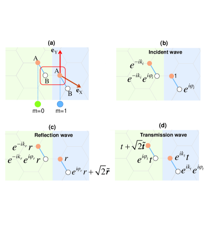
Figure 4: (a) Continuity of the scattering wave function at the interface unit cells $m=0$ and $1$. Each unit cell contains two atoms, as connected by the thick solid line. (b)-(d) show the amplitudes of the incident, reflection, and transmission waves at each carbon site.

Next we discuss the mode-matching condition at the interface $m=0,1$ (see Fig. 4) in more detail to explain why the “abnormal” evanescent eigenstates do not affect the transmission of the traveling eigenstate. The key is that the 2$\times$1 spinor $|\Phi\rangle=[a,b]^{T}$ means that the wave amplitude at the $A$ site is $a$, while that at the $B$ site is $b$. Therefore, the matching of the 2$\times$1 spinor wave function at $m=0$ and $1$ amounts to the matching of the wave amplitudes at the four sites in Fig. 4: Eq. (22a) [Eq. (22b)] for the matching at the $A$ ($B$) site of unit cell $m=1$ and Eq. (23a) [Eq. (23b)] for the matching at the $A$ ($B$) site of $m=0$. However, the left-going ideal evanescent state $|\Phi_{\infty}(m|1)\rangle$ contained in $|\Phi_{r}(m)\rangle$ is nonzero only on the $B$ site of $m=1$, while the right-going ideal evanescent eigenstate $|\Phi_{0}(m|0)\rangle$ contained in $|\Phi_{t}(m)\rangle$ is nonzero only on the $A$ site of $m=0$. Therefore, the matching conditions on the $A$ site of $m=1$ [Eq. (22a)] and on the $B$ site of $m=0$ [Eq. (23b)], as enclosed by the red box in Fig. 4, do not contain any “abnormal” evanescent waves. The matching of the traveling waves at these two sites uniquely determines the reflection and transmission coefficients $r$ and $t$ for the traveling eigenstates.

II.3 Generalized pseudospin in tight-binding model

In the linear continuum model, the perfect Klein tunneling at normal incidence has a physically transparent interpretation as the conservation of the pseudospin Katsnelson et al. (2006); Beenakker (2008); Culcer and Winkler (2008). In the tight-binding model, however, such a simple physical picture for the Klein tunneling is still lacking, due to the broken chirality of the Dirac fermions by the trigonal warping Ajiki and Ando (1996); Ando et al. (1998); Wu et al. (2007); Dombrowski et al. (2017).

Here we demonstrate that in the tight-binding model, the perfect transmission over the energy range $E\in[-1,+1]$ can always be interpreted as the conservation of a generalized pseudospin. The key is that the mode-matching conditions for the traveling waves at the interface form a closed set of equations [Eqs. (22a) and (23b)], which can be put into the form

$$|u_{i}\rangle+r|u_{r}\rangle=te^{ik_{X,t}}|u_{t}\rangle,$$ (27)

where

$$|u_{\alpha}\rangle\equiv\begin{bmatrix}1\\ e^{i(\varphi_{\alpha}-k_{X,\alpha})}\end{bmatrix}\ \ (\alpha=i,r,t).$$

The perfect transmission condition [Eq. (26)] leads to $|u_{i}\rangle=|u_{t}\rangle\neq|u_{r}\rangle$. Conversely, once $|u_{i}\rangle=|u_{t}\rangle\neq|u_{r}\rangle$, we immediately obtain $r=0$ and hence perfect transmission. Thus we arrive at the following necessary and sufficient condition for perfect transmission:

$$|u_{i}\rangle=|u_{t}\rangle\neq|u_{r}\rangle.$$ (28)

By regarding the $A,B$ sites inside the red box of Fig. 4 as a special unit cell across the interface, $|u_{i}\rangle$, $r|u_{r}\rangle$, and $te^{ik_{X,t}}|u_{t}\rangle$ become the amplitudes of the incident, reflection, and transmission waves inside this unit cell, as shown in Fig. 4(b)-(d). Therefore, Eq. (27) simply expresses the continuity of the scattering wave function inside this special unit cell. Then we can associate each spinor with a generalized pseudospin

$$\boldsymbol{\sigma}_{\alpha}\equiv\frac{\langle u_{\alpha}|\boldsymbol{\hat{\sigma}}|u_{\alpha}\rangle}{\langle u_{\alpha}|u_{\alpha}\rangle}=(\cos(\varphi_{\alpha}-k_{X,\alpha})\mathbf{,}\sin(\varphi_{\alpha}-k_{X,\alpha})),$$ (29)

where $\boldsymbol{\hat{\sigma}}=(\hat{\sigma}_{x},\hat{\sigma}_{y})$ and $\hat{\sigma}_{x,y}$ are Pauli matrices. Then the perfect transmission condition amounts to

$$\boldsymbol{\sigma}_{i}=\boldsymbol{\sigma}_{t}\neq\boldsymbol{\sigma}_{r},$$ (30)

i.e., conservation of the generalized pseudospin across the graphene junctions.

II.4 Generalizations to finite-width junctions

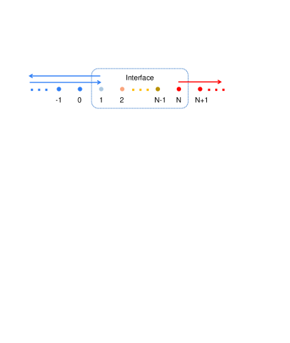
Figure 5: An arbitrary junction consists of the left uniform region ($m\leq 0)$, the interface region ($1\leq m\leq N$), and the right uniform region ($m\geq N+1)$. The arrows indicate the incident wave, the reflection wave, and the transmission wave.

The mode-matching technique in the tilted coordinates can also deal with finite-width junctions. Suppose the left N region, the right P region, and the interface region consist of the unit cells $(m,n)$ with $m\leq 0$, $m\geq N+1$, and $1\leq m\leq N$, respectively. By using the Fourier transform Eq. (2) from the on-site basis into the hybrid basis $|m,k_{Y},\alpha\rangle$, we reduce the 2D junction into a 1D chain parameterized by a given $k_{Y}$. Each unit cell contains two orbitals $A$ and $B$. The 2$\times 2$ on-site energy of the unit cell $m$ is $V_{m}\mathbf{I}_{2\times 2}+\mathbf{h}(k_{Y})$, where the on-site potential $V_{m}=V_{\mathrm{L}}$ in the left N region ($m\leq 0$), $V_{m}=V_{\mathrm{R}}$ in the right P region ($m\geq N+1$), and $V_{m}$ can be arbitrary in the interface region ($1\leq m\leq N$), as shown in Fig. 5(b). The 2$\times$2 hopping from unit cell $m+1$ to $m$ is $\mathbf{t}$ [Eq. (4)].

For a right-going incident wave on the Fermi level from the left N region $|\Phi_{i}(m)\rangle=e^{i(m-1)k_{X,i}}|\Phi_{i}\rangle$, the scattering state is obtained by solving the 1D Schrödinger equation Eq. (15). Solving Eq. (15) with $m\leq 0$ gives

$$|\Psi(m)\rangle=|\Phi_{i}(m)\rangle+re^{i(m-1)k_{X,r}}|\Phi_{r}\rangle+\tilde{r}\lambda_{\infty}^{(m-1)}|\Phi_{\infty}\rangle\ \ (m\leq 1),$$

where the last two terms are reflection waves. Solving Eq. (15) with $m\geq N+1$ gives the transmission waves

$$|\Psi(m)\rangle=te^{i(m-N)k_{X,t}}|\Phi_{X,t}\rangle+\tilde{t}\lambda_{0}^{(m-N)}|\Phi_{0}\rangle\ (m\geq N).$$

The unknown variables$r,\tilde{r},t,\tilde{t}$, and $|\Psi(m)\rangle$ ($2\leq m\leq N-1$) can be uniquely determined by Eq. (15) with $m=1,2,\cdots,N$. This is reminiscent of the mode-matching method developed by Ando Ando (1991), albeit in the tilted coordinates. For large $N$, analytical solutions are no longer available, and numerical calculations are necessary.

III Numerical results and discussions

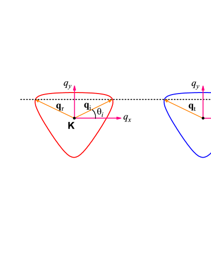
Figure 6: Fermi contours for the N region (conduction band, red contour) and P region (valence band, blue contour) of a symmetric P-N junction with $\varepsilon_{\mathrm{L}}=\varepsilon_{\mathrm{R}}=0.9$. The arrows indicate the reduced wave vectors $\mathbf{q}_{i},\mathbf{q}_{r}$, and $\mathbf{q}_{t}$ for the incident, reflection, and transmission waves.

The mirror symmetry of the P-N junction about the $x$ axis guarantees the transmission probability $T(k_{y})$ to be an even function of $k_{y}$. So we limit our discussions to one valley, say $\mathbf{K}$, and define the reduced wave vector $\mathbf{q}\equiv\mathbf{k}-\mathbf{K}$. For specificity we calculate the transmission probability of electrons in the $\mathbf{K}$ valley across a symmetric graphene P-N junction with $\varepsilon_{\mathrm{L}}=-\varepsilon_{\mathrm{R}}=V_{0}$; i.e., the electron doping in the left N region is equal to the hole doping in the right P region. We present our calculation results in the conventional Cartesian coordinates (see Fig. 1) to make them accessible to readers that are more familiar with the Cartesian coordinates. For a given $q_{y}$, the wave vectors of the incident, reflection, and transmission waves correspond to the intersection points of the horizontal line $q_{y}$ and the Fermi contour in the $(q_{x},q_{y})$ plane, as shown in Fig. 6. The incident wave is characterized by either $q_{y}$ or the azimuth angle $\theta_{i}$ of $\mathbf{q}_{i}$, so the transmission probability is denoted by $T(q_{y})$ or $T(\theta_{i})$. For clarity we define $q_{y,\mathrm{PT}}$ ($\theta_{\mathrm{PT}}$) as the critical momentum (angle) leading to perfect transmission: $T(q_{y,\mathrm{PT}})=1$ [$T(\theta_{\mathrm{PT}})=1$]. For reference, the conventional continuum model with a linear dispersion gives the transmission probability $T(\theta_{i})=\cos^{2}\theta_{i}$ (Ref. Cheianov and Fal’ko, 2006) and hence $q_{y,\mathrm{PT}}=\theta_{\mathrm{PT}}=0$.

III.1 Numerical results

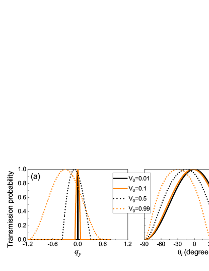
Figure 7: (a) Transmission probability as a function of $q_{y}$. (b) Transmission probability as a function of the azimuth angle $\theta_{i}$ of the incident wave vector $\mathbf{q}_{i}$.

At the beginning, we plot in Fig. 7 the exact results from the tight-binding model for the transmission probability, as calculated from Eqs. (25) and (24). At very low doping $V_{0}=0.01$, perfect transmission occurs at $q_{y,\mathrm{PT}}=\theta_{\mathrm{PT}}=0$, in agreement with the well-known Klein tunneling in the widely used linear continuum model Katsnelson et al. (2006). However, with increasing doping level, $q_{y,\mathrm{PT}}$ and $\theta_{\mathrm{PT}}$ exhibit larger and larger deviations from zero, indicating perfect transmission at oblique incidence.

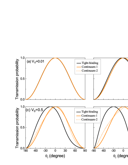
Figure 8: Transmission probability from the tight-binding model vs those from the linear continuum model (solid orange line) or with quadratic corrections (dashed orange line) for different doping levels: (a) $V_{0}=0.01$, (b) $V_{0}=0.1$, (c) $V_{0}=0.5$, and (d) $V_{0}=0.99$.

In Fig. 8, we compare the exact results from the tight-binding model to those from the continuum models. At very low doping $V_{0}=0.01$ [Fig. 8(a)], all the models agree with each other and give $\theta_{\mathrm{PT}}=0$. However, with increasing doping level, the results from the continuum models deviate more and more from the exact results. Actually, the deviation is appreciable even at relatively low doping $V_{0}=0.1$ [Fig. 8(b)], where the trigonal warping is small: $\eta=3\%$ [Fig. 1(c)]. Interestingly, even the continuum model with a quadratic correction (dashed orange line) to incorporate the trigonal warping up to the lowest order (see the Appendix) does not agree with the exact results.

Figure 9: Fermi contours for each region of the graphene P-N junction in the Cartesian coordinate $(q_{x},q_{y})$ for different doping levels: (a) $V_{0}=0.01$ and (b) $V_{0}=0.5$. Red (blue) for right-going (left-going) states and arrows for their pseudospins. In each panel, the inset shows the transmission probability $T(\theta_{i})$ as a function of the azimuth angle $\theta_{i}$ of the incident wave vector $\mathbf{q}_{i}$.

Next we illustrate the generalized pseudospin picture (see Sec. II.3) in the tight-binding model. As shown in Fig. 9, for a given $q_{y}$, the wave vectors $\mathbf{q}_{i},\mathbf{q}_{r},\mathbf{q}_{t}$ of the incident, reflection, and transmission waves are obtained as the intersection points between a horizontal line (see the orange dashed line for an example) corresponding to this $q_{y}$ and the Fermi contour. For low doping $V_{0}=0.01$, the condition $\boldsymbol{\sigma}_{i}=\boldsymbol{\sigma}_{t}\neq\boldsymbol{\sigma}_{r}$ is satisfied at $q_{y}=0$, so perfect transmission occurs at normal incidence $\theta_{\mathrm{PT}}=0$ [Fig. 9(a)]. For higher doping $V_{0}=0.5$ [Fig. 9(b)], the texture of the generalized pseudospins on the Fermi contour is twisted relative to those at low doping. In this case, the condition $\boldsymbol{\sigma}_{i}=\boldsymbol{\sigma}_{t}\neq\boldsymbol{\sigma}_{r}$ occurs at $\theta_{\mathrm{PT}}\approx-14.6\operatorname{{{}^{\circ}}}$; i.e., perfect transmission occurs for oblique incidence.

III.2 Experimental feasibility

Ever since the initial theoretical prediction Katsnelson et al. (2006), many experimental efforts Huard et al. (2007); Gorbachev et al. (2008); Stander et al. (2009); Young and Kim (2009); Rossi et al. (2010); Sajjad et al. (2012); Sutar et al. (2012); Rahman et al. (2015); Guti rrez et al. (2016); Chen et al. (2016); Bai et al. (2017) have been devoted to Klein tunneling in graphene, culminating in the experimental demonstration of the prominent angular dependence of the transmission probability in graphene P-N junctions Sajjad et al. (2012); Sutar et al. (2012); Rahman et al. (2015); Chen et al. (2016). In particular, the recent fabrication of high-quality graphene P-N junctions with high doping levels Dombrowski et al. (2017) makes the high-energy transmission across graphene P-N junctions experimentally accessible; e.g., the perfect transmission angle $\theta_{\mathrm{PT}}$ may be extracted by measuring the angular dependence of transmission probability. To serve future experiments, we plot the perfect transmission momentum $q_{y,\mathrm{PT}}$ and the perfect transmission angle $\theta_{\mathrm{PT}}$ as functions of the doping level $V_{0}$ in Fig. 10.

Up to now, we have focused on symmetric P-N junctions with a sharp interface and equal doping level and trigonal warping on both sides. For asymmetric P-N junctions, the trigonal warping in the N region is not equal to that in the P region. This may weaken the effect of perfect transmission at oblique incidence by shifting $\theta_{\mathrm{PT}}$ towards zero. A smooth junction potential usually suppresses the transmission as the incident angle increases Cheianov and Fal’ko (2006) and plays an important role in the electron optics in the graphene P-N junction Chen et al. (2016). This may hinder the experimental observation of perfect transmission at oblique incidence. Fortunately, a very recent experiment Bai et al. (2017) shows that atomically sharp graphene P-N junctions can be fabricated on the copper surface. The potential difference between the P and the N regions can reach $2V_{0}=660$ meV, corresponding to a doping level $V_{0}=0.33$ eV and doping density $10^{13}$ cm^-2 [see the inset of Fig. 10(b)]. At this doping level, the trigonal warping is $\eta=4\%$ and the perfect transmission angle is $\theta_{\mathrm{PT}}\approx-3.5\operatorname{{{}^{\circ}}}$. Moreover, a previous theoretical study shows that the electron-electron interaction Roldán et al. (2008) generally enhances the trigonal warping. Therefore, we expect the perfect transmission at oblique incidence to be experimentally accessible in the near future.

Finally, we note the intensive experimental activities in simulating the honeycomb lattices by cold atoms and optical lattices Polini et al. (2013). In particular, the possibility of Klein tunneling in these system has been examined Longhi (2010); Casanova et al. (2010); Zhang et al. (2012); Fang et al. (2016); Ozawa et al. (2017) and observed recently Gerritsma et al. (2011); Salger et al. (2011). These simulated graphene systems may provide an alternative platform for observing the perfect transmission at oblique incidence. It would also be interesting to explore the effect of trigonal warping on the transmission across bilayer graphene P-N junctions Tudorovskiy et al. (2012); Culcer and Winkler (2009).

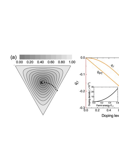
Figure 10: (a) Incident wave vector (black dots) on the Fermi contour leading to perfect transmission under different doping levels $V_{0}$. (b) Critical momentum $q_{y,\mathrm{PT}}$ and angle $\theta_{\mathrm{PT}}$ for perfect transmission as functions of the doping level. The inset shows the doping density vs. the Fermi energy, as calculated from the tight-binding model.

IV Conclusions

We have developed an analytical mode-matching technique to study the electron transmission across graphene P-N junctions over a wide energy range. In contrast to the well-known Klein tunneling at normal incidence for low energies in the linear Dirac regime, we find that at energies beyond the linear Dirac regime, the Klein tunneling at normal incidence becomes imperfect and trigonal warping causes perfect transmission at oblique incidence. We show that this phenomenon arises from the conservation of a generalized pseudospin in the tight-binding model. This generalizes the well-known pseudospin picture for perfect Klein tunneling, previously limited to low energies in the linear Dirac regime, to all the energy ranges. The perfect transmission at oblique incidence cannot be described by the continuum model, even after quadratic corrections have been introduced to incorporate trigonal warping up to the leading order. Our work may be relevant for the applications of the graphene P-N junction in electronics and electron optics.

Appendix A Hamiltonian of uniform graphene in Cartesian coordinates

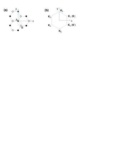
Figure 11: (a) Lattice structure of graphene: filled (empty) circles for sublattice $A$ ($B$). (b) Six Dirac points at the edge of the first Brillouin zone of graphene.

As shown in Fig. 11(a), the honeycomb lattice of graphene consists of two sublattices (denoted by $A$ and $B$) and each unit cell contains two carbon atoms (or $\pi_{z}$-orbitals), one on each sublattice. The tight-binding Hamiltonian of graphene is

$$\hat{H}_{0}=-\sum_{\left\langle i,j\right\rangle}|i,A\rangle\langle j,B|-h.c.,$$

where $\langle i,j\rangle$ sums over all the nearest-neighbor carbon pairs, $|i,\lambda\rangle$ ($\lambda=A,B$) is the $\pi_{z}$ orbital on the sublattice $\lambda$ of unit cell $i$, and we have taken the nearest-neighbor hopping energy as the unit of energy. We take the $A$ site as the origin of each unit cell, so the relative displacements of the two carbon atoms inside the unit cell are $\boldsymbol{\tau}_{A}=0$ and $\boldsymbol{\tau}_{B}=(1/2,-\sqrt{3}/2)$, where we have taken the carbon-carbon bond length as the unit of length. In terms of the unit cell location $\mathbf{R}_{i}$, the location of the site $\lambda$ in unit cell $i$ is $\mathbf{R}_{i,\lambda}=\mathbf{R}_{i}+\boldsymbol{\tau}_{\lambda}$.

By Fourier transforming the real-space basis $\{|i,\lambda\rangle\}$ into the momentum space basis $\{|\mathbf{k},\lambda\rangle\}$, the graphene Hamiltonian can be transformed into the momentum space:

$$\hat{H}_{0}=\sum_{\mathbf{k}}f(\mathbf{k})|\mathbf{k},A\rangle\langle\mathbf{k},B|+h.c.,$$

where $f(\mathbf{k)}=-\sum_{i=1,2,3}e^{i\mathbf{k}\cdot\mathbf{d}_{i}}$ and $\{\mathbf{d}_{i}\}$ depend on the choices on the Fourier transform. Namely, if we make the Fourier transform using the location $\{\mathbf{R}_{i\lambda}\}$ of the carbon sites:

$$|\mathbf{k},\lambda\rangle_{\mathrm{I}}\equiv\frac{1}{\sqrt{N}}\sum_{i}e^{i\mathbf{k}\cdot\mathbf{R}_{i\lambda}}|i,\lambda\rangle,$$

then $\mathbf{d}_{1},\mathbf{d}_{2},\mathbf{d}_{3}$ denote the relative displacements of the three nearest-neighbor $B$ sites [empty circles in Fig. 11(a)] with respect to the central $A$ site [blue filled circle in Fig. 11(a)]:

$$\mathbf{d}_{1}^{\mathrm{I}}=\boldsymbol{\tau}_{B},\ \ \mathbf{d}_{2}^{\mathrm{I}}=\left(\frac{1}{2},\frac{\sqrt{3}}{2}\right),\ \ \mathbf{d}_{3}^{\mathrm{I}}=\left(-1,0\right).$$

However, if we make the Fourier transform using the location $\{\mathbf{R}_{i}\}$ of the unit cells:

$$|\mathbf{k},\lambda\rangle_{\mathrm{II}}\equiv\frac{1}{\sqrt{N}}\sum_{i}e^{i\mathbf{k}\cdot\mathbf{R}_{i}}|i,\lambda\rangle,$$

then $\mathbf{d}_{1},\mathbf{d}_{2},\mathbf{d}_{3}$ denote the relative displacements of the three nearest-neighbor unit cells [black filled circles in Fig. 11(a)] with respect to the central unit cell [blue filled circle in Fig. 11(a)]:

$$\mathbf{d}_{1}^{\mathrm{II}}=0,\ \ \ \mathbf{d}_{2}^{\mathrm{II}}=(0,\sqrt{3})\text{,}\ \ \ \mathbf{d}_{3}^{\mathrm{II}}=\left(-\frac{3}{2},\frac{\sqrt{3}}{2}\right).$$

These two choices are connected by $|\mathbf{k},A\rangle_{\mathrm{II}}=|\mathbf{k},A\rangle_{\mathrm{I}}$, $|\mathbf{k},B\rangle_{\mathrm{II}}=e^{-i\mathbf{k}\cdot\boldsymbol{\tau}_{B}}|\mathbf{k},B\rangle_{\mathrm{I}}$, $\mathbf{d}_{i}^{\mathrm{II}}=\mathbf{d}_{i}^{\mathrm{I}}-\boldsymbol{\tau}_{B}$, and $f_{\mathrm{II}}(\mathbf{k})=$ $e^{-i\mathbf{k}\cdot\boldsymbol{\tau}_{B}}f_{\mathrm{I}}(\mathbf{k})$. Both cases satisfy $f^{\ast}(-\mathbf{k})=f(\mathbf{k})$; thus under time-reversal operation $\hat{\theta}$, which leaves $|i\lambda\rangle$ invariant and brings $|\mathbf{k},\lambda\rangle$ into $\hat{\theta}|\mathbf{k},\lambda\rangle=|-\mathbf{k,}\lambda\rangle$, the graphene Hamiltonian remains invariant:

$$\hat{\theta}\hat{H}_{0}\hat{\theta}^{-1}=\sum_{\mathbf{k}}f^{\ast}(\mathbf{k})|-\mathbf{k},A\rangle\langle-\mathbf{k},B|+h.c.=\hat{H}_{0}.$$

Diagonalizing the Hamiltonian in the momentum space gives one conduction band and one valence band $E_{\pm}(\mathbf{k})=\pm|f(\mathbf{k})|$ or explicitly

$$E_{\pm}(\mathbf{k})=\pm\sqrt{3+2\cos(\sqrt{3}k_{y})+4\cos\frac{3k_{x}}{2}\cos\frac{\sqrt{3}k_{y}}{2}},$$ (31)

which touch each other (i.e., $f(\mathbf{k})=0$) at six Dirac points at the edge of the first Brillouin zone [Fig. 11(b)]. Since $\mathbf{K}_{1},\mathbf{K}_{3},\mathbf{K}_{5}$ ($\mathbf{K}_{2},\mathbf{K}_{4},\mathbf{K}_{6}$) only differ by a reciprocal vector, only two Dirac points are inequivalent, e.g., $\mathbf{K}_{1}$ and $\mathbf{K}_{2}$. Hereafter we denote $\mathbf{K}_{1}$ as $\mathbf{K}$ and $\mathbf{K}_{2}$ as $\mathbf{K}^{\prime}$:

$$\mathbf{K}=\frac{2\pi}{3}\left(1,\frac{1}{\sqrt{3}}\right),\mathbf{K}^{\prime}=\frac{2\pi}{3}\left(1,-\frac{1}{\sqrt{3}}\right).$$

The continuum model near the Dirac point $\mathbf{K}_{j}$ is obtained by considering $\mathbf{k}\approx\mathbf{K}_{j}$ and expanding $f(\mathbf{k})$ into Taylor series of $\mathbf{q}\equiv\mathbf{k}-\mathbf{K}_{j}$:

$$\hat{H}_{j}(\mathbf{q})=\sum_{\mathbf{q}}f_{j}(\mathbf{q})|\mathbf{K}_{j},A\rangle\langle\mathbf{K}_{j},B|+h.c.,$$

where $f_{j}(\mathbf{q})\equiv f(\mathbf{K}_{j}+\mathbf{q})$. Up to the second order of $\mathbf{q}$, we have

$$f_{1,\mathrm{I}}(\mathbf{q}) =f_{4,\mathrm{I}}^{\ast}(-\mathbf{q})=\frac{3}{2}qe^{-i\pi/6+i\theta_{\mathbf{q}}}-\frac{3}{8}q^{2}e^{i\pi/3}e^{-i2\theta_{\mathbf{q}}},$$

$$f_{2,\mathrm{I}}(\mathbf{q}) =f_{5,\mathrm{I}}^{\ast}(-\mathbf{q})=\frac{3}{2}qe^{-i\pi/6\mathbf{-}i\theta_{\mathbf{q}}}-\frac{3}{8}q^{2}e^{i\pi/3}e^{i2\theta_{\mathbf{q}}},$$

$$f_{3,\mathrm{I}}(\mathbf{q}) =f_{6,\mathrm{I}}^{\ast}(-\mathbf{q})=\frac{3}{2}iqe^{i\theta_{\mathbf{q}}}+\frac{3}{8}q^{2}e^{-i2\theta_{\mathbf{q}}},$$

for choice I, where $\theta_{\mathbf{q}}$ is the azimuthal angle of $\mathbf{q}$. This choice gives a concise form for the $O(q^{2})$ terms, so it is usually used to study the trigonal warping effect of graphene Reijnders and Katsnelson (2017). For choice II, the $O(q^{2})$ term is very complicated (although different choices of the Fourier transform give the same physics Bena and Montambaux (2009)), so we only give the Taylor expansion up to $O(q)$:

$$f_{1,\mathrm{II}}(\mathbf{q}) =f_{3,\mathrm{II}}(\mathbf{q})=f_{5,\mathrm{II}}(\mathbf{q})=\frac{3}{2}qe^{-i\pi/6+i\theta_{\mathbf{q}}},$$

$$f_{2,\mathrm{II}}(\mathbf{q}) =f_{4,\mathrm{II}}(\mathbf{q})=f_{6,\mathrm{II}}(\mathbf{q})=-\frac{3}{2}qe^{i\pi/6-i\theta_{\mathbf{q}}}.$$

For either case, we have the identity $f_{i+3}(\mathbf{q})=f_{i}^{\ast}(-\mathbf{q})$, which follows from the time-reversal symmetry $f^{\ast}(-\mathbf{k})=f(\mathbf{k})$.

References

- Klein (1929) O. Klein, Zeitschrift für Physik 53, 157 (1929).
- Allain and Fuchs (2011) P. E. Allain and J. Fuchs, The European Physical Journal B 83, 301 (2011).
- Katsnelson et al. (2006) M. I. Katsnelson, K. S. Novoselov, and A. K. Geim, Nat. Phys. 2, 620 (2006).
- Cheianov and Fal’ko (2006) V. V. Cheianov and V. I. Fal’ko, Phys. Rev. B 74, 041403 (2006).
- Pereira et al. (2006) J. M. Pereira, V. Mlinar, F. M. Peeters, and P. Vasilopoulos, Phys. Rev. B 74, 045424 (2006).
- Bai and Zhang (2007) C. Bai and X. Zhang, Phys. Rev. B 76, 075430 (2007).
- Beenakker et al. (2008) C. W. J. Beenakker, A. R. Akhmerov, P. Recher, and J. Tworzydło, Phys. Rev. B 77, 075409 (2008).
- Setare and Jahani (2010) M. R. Setare and D. Jahani, J. Phys. Condens. Matter 22, 245503 (2010).
- Roslyak et al. (2010) O. Roslyak, A. Iurov, G. Gumbs, and D. Huang, J. Phys. Condens. Matter 22, 165301 (2010).
- Zeb et al. (2008) M. A. Zeb, K. Sabeeh, and M. Tahir, Phys. Rev. B 78, 165420 (2008).
- Sonin (2009) E. B. Sonin, Phys. Rev. B 79, 195438 (2009).
- Schelter et al. (2010) J. Schelter, D. Bohr, and B. Trauzettel, Phys. Rev. B 81, 195441 (2010).
- Yang et al. (2011) R. Yang, L. Huang, Y.-C. Lai, and C. Grebogi, Phys. Rev. B 84, 035426 (2011).
- Rozhkov et al. (2011) A. Rozhkov, G. Giavaras, Y. P. Bliokh, V. Freilikher, and F. Nori, Phys. Rep. 503, 77 (2011).
- Liu et al. (2012) M.-H. Liu, J. Bundesmann, and K. Richter, Phys. Rev. B 85, 085406 (2012).
- Giavaras and Nori (2012) G. Giavaras and F. Nori, Phys. Rev. B 85, 165446 (2012).
- Rodriguez-Vargas et al. (2012) I. Rodriguez-Vargas, J. Madrigal-Melchor, and O. Oubram, J. Appl. Phys. 112, 073711 (2012).
- Popovici et al. (2012) C. Popovici, O. Oliveira, W. de Paula, and T. Frederico, Phys. Rev. B 85, 235424 (2012).
- Heinisch et al. (2013) R. L. Heinisch, F. X. Bronold, and H. Fehske, Phys. Rev. B 87, 155409 (2013).
- Logemann et al. (2015) R. Logemann, K. J. A. Reijnders, T. Tudorovskiy, M. I. Katsnelson, and S. Yuan, Phys. Rev. B 91, 045420 (2015).
- Oh et al. (2016) H. Oh, S. Coh, Y.-W. Son, and M. L. Cohen, Phys. Rev. Lett. 117, 016804 (2016).
- Erementchouk et al. (2016) M. Erementchouk, P. Mazumder, M. A. Khan, and M. N. Leuenberger, J. Phys. Condens. Matter 28, 115501 (2016).
- Downing and Portnoi (2017) C. A. Downing and M. E. Portnoi, J. Phys. Condens. Matter 29, 315301 (2017).
- Huard et al. (2007) B. Huard, J. A. Sulpizio, N. Stander, K. Todd, B. Yang, and D. Goldhaber-Gordon, Phys. Rev. Lett. 98, 236803 (2007).
- Gorbachev et al. (2008) R. V. Gorbachev, A. S. Mayorov, A. K. Savchenko, D. W. Horsell, and F. Guinea, Nano Lett. 8, 1995 (2008).
- Stander et al. (2009) N. Stander, B. Huard, and D. Goldhaber-Gordon, Phys. Rev. Lett. 102, 026807 (2009).
- Young and Kim (2009) A. F. Young and P. Kim, Nat. Phys. 5, 222 (2009).
- Rossi et al. (2010) E. Rossi, J. H. Bardarson, P. W. Brouwer, and S. Das Sarma, Phys. Rev. B 81, 121408 (2010).
- Sajjad et al. (2012) R. N. Sajjad, S. Sutar, J. U. Lee, and A. W. Ghosh, Phys. Rev. B 86, 155412 (2012).
- Sutar et al. (2012) S. Sutar, E. S. Comfort, J. Liu, T. Taniguchi, K. Watanabe, and J. U. Lee, Nano Lett. 12, 4460 (2012).
- Rahman et al. (2015) A. Rahman, J. W. Guikema, N. M. Hassan, and N. Marković, Appl. Phys. Lett. 106, 013112 (2015).
- Guti rrez et al. (2016) C. Guti rrez, L. Brown, C. J. Kim, J. Park, and A. N. Pasupathy, Nat. Phys. 12, 1069 (2016).
- Chen et al. (2016) S. Chen, Z. Han, M. M. Elahi, K. M. M. Habib, L. Wang, B. Wen, Y. Gao, T. Taniguchi, K. Watanabe, J. Hone, et al., Science 353, 1522 (2016).
- Laitinen et al. (2016) A. Laitinen, G. S. Paraoanu, M. Oksanen, M. F. Craciun, S. Russo, E. Sonin, and P. Hakonen, Phys. Rev. B 93, 115413 (2016).
- Bai et al. (2017) K.-K. Bai, J.-B. Qiao, H. Jiang, H. Liu, and L. He, Phys. Rev. B 95, 201406 (2017).
- Sajjad and Ghosh (2011) R. N. Sajjad and A. W. Ghosh, Appl. Phys. Lett. 99, 123101 (2011).
- Jang et al. (2013) M. S. Jang, H. Kim, Y.-W. Son, H. A. Atwater, and W. A. Goddard, Proc. Natl. Acad. Sci. 110, 8786 (2013).
- Wilmart et al. (2014) Q. Wilmart, S. Berrada, D. Torrin, V. H. Nguyen, G. Fève, J.-M. Berroir, P. Dollfus, and B. Plaçais, 2D Materials 1, 011006 (2014).
- Chen and Chang (2015) C.-C. Chen and Y.-C. Chang, Phys. Rev. B 92, 245406 (2015).
- de Sousa et al. (2017) D. J. P. de Sousa, A. Chaves, J. M. PereiraJr., and G. A. Farias, J. Appl. Phys. 121, 024302 (2017).
- Tan et al. (2017) Y. Tan, M. M. Elahi, H.-Y. Tsao, K. M. M. Habib, N. S. Barker, and A. W. Ghosh, Scientific Reports 7, 9714 (2017).
- Bir and Pikus (1974) G. Bir and G. Pikus, Symmetry and Strain-induced Effects in Semiconductors (Wiley, New York, 1974).
- Castro Neto et al. (2009) A. H. Castro Neto, F. Guinea, N. M. R. Peres, K. S. Novoselov, and A. K. Geim, Rev. Mod. Phys. 81, 109 (2009).
- Wu et al. (2007) X. Wu, X. Li, Z. Song, C. Berger, and W. A. de Heer, Phys. Rev. Lett. 98, 136801 (2007).
- Dombrowski et al. (2017) D. Dombrowski, W. Jolie, M. Petrovi, S. Runte, F. Craes, J. Klinkhammer, M. Kralj, P. Lazić, E. Sela, and C. Busse, Phys. Rev. Lett. 118, 116401 (2017).
- Xing et al. (2010) Y. Xing, J. Wang, and Q.-f. Sun, Phys. Rev. B 81, 165425 (2010).
- Reijnders and Katsnelson (2017) K. J. A. Reijnders and M. I. Katsnelson, Phys. Rev. B 96, 045305 (2017).
- Cheianov et al. (2007) V. V. Cheianov, V. Fal’ko, and B. L. Altshuler, Science 315, 1252 (2007).
- Lee et al. (2015) G.-H. Lee, G.-H. Park, and H.-J. Lee, Nat. Phys. 11, 925 (2015).
- Garcia-Pomar et al. (2008) J. L. Garcia-Pomar, A. Cortijo, and M. Nieto-Vesperinas, Phys. Rev. Lett. 100, 236801 (2008).
- Jr et al. (2009) J. M. P. Jr, F. M. Peeters, R. N. C. Filho, and G. A. Farias, J. Phys. Condens. Matter 21, 045301 (2009).
- Reich et al. (2002) S. Reich, J. Maultzsch, C. Thomsen, and P. Ordejón, Phys. Rev. B 66, 035412 (2002).
- Datta (1995) S. Datta, Electronic Transport in Mesoscopic Systems (Cambridge University Press, Cambridge, England, 1995).
- Ferry and Goodnick (1997) D. Ferry and S. Goodnick, Transport in Nanostructures (Cambridge University Press, Cambridge, 1997).
- Lewenkopf and Mucciolo (2013) C. H. Lewenkopf and E. R. Mucciolo, Journal of Computational Electronics 12, 203 (2013).
- Zhang et al. (2017) S.-H. Zhang, W. Yang, and K. Chang, Phys. Rev. B 95, 075421 (2017).
- Beenakker (2008) C. W. J. Beenakker, Rev. Mod. Phys. 80, 1337 (2008).
- Ando (1991) T. Ando, Phys. Rev. B 44, 8017 (1991).
- Culcer and Winkler (2008) D. Culcer and R. Winkler, Phys. Rev. B 78, 235417 (2008).
- Ajiki and Ando (1996) H. Ajiki and T. Ando, J. Phys. Soc. Jpn. 65, 505 (1996).
- Ando et al. (1998) T. Ando, T. Nakanishi, and R. Saito, J. Phys. Soc. Jpn. 67, 2857 (1998).
- Bai et al. (2017) K.-K. Bai, J.-J. Zhou, Y.-C. Wei, J.-B. Qiao, Y.-W. Liu, H.-W. Liu, H. Jiang, and L. He, arXiv:1705.10952 [cond-mat.mes-hall] (2017), eprint 1705.10952.
- Roldán et al. (2008) R. Roldán, M. P. López-Sancho, and F. Guinea, Phys. Rev. B 77, 115410 (2008).
- Polini et al. (2013) M. Polini, F. Guinea, M. Lewenstein, H. C. Manoharan, and V. Pellegrini, Nat Nano 8, 625 (2013).
- Longhi (2010) S. Longhi, Phys. Rev. B 81, 075102 (2010).
- Casanova et al. (2010) J. Casanova, J. J. García-Ripoll, R. Gerritsma, C. F. Roos, and E. Solano, Phys. Rev. A 82, 020101 (2010).
- Zhang et al. (2012) D.-W. Zhang, Z.-Y. Xue, H. Yan, Z. D. Wang, and S.-L. Zhu, Phys. Rev. A 85, 013628 (2012).
- Fang et al. (2016) A. Fang, Z. Q. Zhang, S. G. Louie, and C. T. Chan, Phys. Rev. B 93, 035422 (2016).
- Ozawa et al. (2017) T. Ozawa, A. Amo, J. Bloch, and I. Carusotto, Phys. Rev. A 96, 013813 (2017).
- Gerritsma et al. (2011) R. Gerritsma, B. P. Lanyon, G. Kirchmair, F. Zähringer, C. Hempel, J. Casanova, J. J. García-Ripoll, E. Solano, R. Blatt, and C. F. Roos, Phys. Rev. Lett. 106, 060503 (2011).
- Salger et al. (2011) T. Salger, C. Grossert, S. Kling, and M. Weitz, Phys. Rev. Lett. 107, 240401 (2011).
- Tudorovskiy et al. (2012) T. Tudorovskiy, K. J. A. Reijnders, and M. I. Katsnelson, Phys. Scr. T146, 014010 (2012).
- Culcer and Winkler (2009) D. Culcer and R. Winkler, Phys. Rev. B 79, 165422 (2009).
- Bena and Montambaux (2009) C. Bena and G. Montambaux, New J. Phys. 11, 095003 (2009).