Reconstructing a cascade from temporal observations

Abstract

Given a subset of active nodes in a network can we reconstruct the cascade that has generated these observations? This is a problem that has been studied in the literature, but here we focus in the case that temporal information is available about the active nodes. In particular, we assume that in addition to the subset of active nodes we also know their activation time.

We formulate this cascade-reconstruction problem as a variant of a Steiner-tree problem: we ask to find a tree that spans all reported active nodes while satisfying temporal-consistency constraints. We present three approximation algorithms. The best algorithm in terms of quality achieves a $\mathcal{O}(\sqrt{k})$-approximation guarantee, where $k$ is the number of active nodes, while the most efficient algorithm has linearithmic running time, making it scalable to very large graphs.

We evaluate our algorithms on real-world networks with both simulated and real cascades. Our results indicate that utilizing the available temporal information allows for more accurate cascade reconstruction. Furthermore, our objective leads to finding the “backbone” of the cascade and it gives solutions of high precision.

1 Introduction

Ideas, behaviors, computer viruses, and diseases, spread in networks. People are influencing each other adopting behaviors, innovations, or memes. Diseases like flu or measles are transmitted from person to person, while computer viruses spread in computer networks. The study of diffusion processes has been a central theme in network science and graph mining. Topics of interest include modeling diffusion processes [1, 2, 3], devising strategies to contain the spread of epidemics [4, 5], maximizing the spread of influence for marketing purposes [2], as well as identifying starting points and missing nodes in cascades [6, 7, 8, 9, 10, 11, 12, 13].

In this paper we consider the problem of reconstructing a cascade that has occurred in a network, given partial observations. We model the problem by considering a graph $G=(V,E)$ and a subset of nodes $V^{\prime}\subseteq V$ that have been activated/infected during the cascade (people who have fallen sick, users who have adopted an innovation, etc.). The goal is to infer the hidden cascade and reconstruct other possible active nodes. Previous approaches on this problem make assumptions about the underlying diffusion models, such as the susceptible-infected model (si) [9, 12] or the independent-cascade model (ic) [8], or consider additional information, such as the exact time of all network interactions [10].

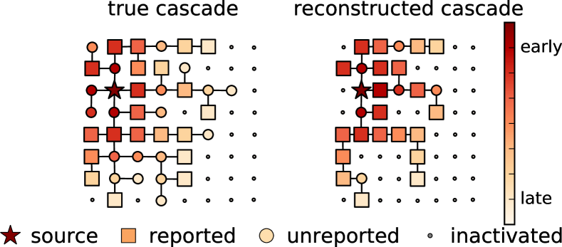
Figure 1: Our method aims at reconstructing the underlying cascade given reported infections (left). The reconstructed cascade (right) is parsimonious and respects node infection order induced by infection time. Node infection time is indicated by the colorbar.

Our approach to the cascade-reconstruction problem is to utilize temporal information about the active nodes. In particular, we consider that for all observed active nodes the activation time is known. This is a realistic assumption in many settings, e.g., it is often easy to determine when a patient got sick. However, we still consider the case of partial observations, i.e., $V^{\prime}$ is a subset of all active nodes in the cascade.

A simple example is illustrated in Figure 1. A ground truth cascade is depicted in the left side. Only a subset of the infected nodes are known, and for those nodes we also know their infection time, which is indicated by the colorbar in the right. A cascade reconstructed by our algorithms, for this problem instance, is shown in the right side. The reconstructed cascade is required to parsimonious and to respect the node infecting order induced by the input infection times. We note that we do not make any assumption about the diffusion model; we only rely on parsimony and ask to find the smallest cascade tree that is consistent with the observed data. Formulated in this manner, our approach is able to find the most important nodes of the cascade and thus, it gives solutions of high precision.

From the technical viewpoint, we formulate the cascade-reconstruction problem as a Steiner-tree problem. Given the reported active nodes and their activation timestamps, we seek to find a tree that spans all reported nodes, while all rooted paths in the tree preserve the order of the observed timestamps. We refer to such a tree by order-preserving Steiner tree and to the problem we study by OrderedSteinerTree. This is a novel Steiner-tree problem variant.

For the proposed problem we develop three approximation algorithms. The first algorithm, closure, uses the metric closure of the graph induced by the reported active nodes: it constructs a directed graph, finds a minimum spanning tree on that graph, and builds a cascade tree based on the minimum spanning tree. The second algorithm, greedy, is a simplification of closure and it builds a cascade tree directly from the reported active nodes, without finding a minimum spanning tree on the metric closure. The third algorithm, delayed-bfs, builds the cascade tree by a modified breadth-first search (bfs) that takes into account the activation timestamps to delay certain search branches.

All three algorithms come with provable approximation guarantees. Assuming that the number of reported active nodes is $k$, closure provides a $\mathcal{O}(\sqrt{k})$-approximation guarantee while both greedy and delayed-bfs give a $k$-approximation guarantee. In practice, when compared to a lower-bound obtained by the standard (non-temporal) Steiner-tree problem, all three algorithms give much better solutions than it is suggested by the theoretical guarantee.

In terms of scalability, the running time of closure and greedy is $\mathcal{O}(km+k^{2})$ and $\mathcal{O}(km)$ respectively, where $m$ is the number of edges of the graph $G$. On the other hand, delayed-bfs runs in time $\mathcal{O}(m+k\log k)$, making it an extremely scalable algorithm, able to cope with very large graphs and large number of reported active nodes.

In summary, our contributions are as follows.

• We present a novel formulation of a Steiner-tree problem with ordering constraints, which models the problem of reconstructing a cascade from partial observations with temporal information.

• For the proposed Steiner-tree problem we provide three approximation algorithms. The best algorithm in terms of quality achieves a $\mathcal{O}(\sqrt{k})$-approximation guarantee and has running time $\mathcal{O}(km)$. The most scalable algorithm achieves a $k$-approximation guarantee and has running time $\mathcal{O}(m+k\log k)$.

• We experimentally evaluate the proposed algorithms on real-world networks using cascades simulated with different diffusion models. Comparison with the baseline Steiner-tree algorithm that does not use temporal information, shows that incorporating timestamps in the problem setting does not lead to significant loss in solution quality (as measured by the objective function) while allowing to find other active nodes with better predicted activation time.

The rest of the paper is organized as follows. First, we discuss the related work in Section 2. Then we introduce necessary notation and definitions in Section 3. Section 4 presents the problem formulation, followed by Section 5 where we discuss and analyze our approximation algorithms. In Section 6, we evaluate the performance of the proposed algorithms, and Section 7 concludes the paper.

2 Related work

Diffusion processes have been widely studied in general. However, the problem of “reverse engineering” an epidemic has received relatively little attention. Shah and Zaman [12] formalize the notion of rumor-centrality to identify the single source node of an epidemic under the susceptible-infected model (si), and provide an optimal algorithm for $d$-regular trees. Prakash et al. [9] study the problem of recovering multiple seed nodes under the si model using the minimum-description length principle (mdl) — i.e., as in this paper a parsimony principle is used. Lappas et al. [8] study the problem of identifying $k$ seed nodes, or effectors, in a partially-activated network, which is assumed to be in steady-state under the independent-cascade) model (ic). Feizi et al. [6] and Sefer et al. [14] address the same problem (identifying $k$ seed nodes) in the case of multiple snapshots of a graph. Feizi et al. consider the si model, while Sefer et al. consider the susceptible-exposed-infectious-recovered model (seir) model. These works consider fully-observed infection footprints and focus only on the source-detection problem.

A recent approach on the cascade-reconstruction problem was proposed by Rozenshtein et al. [10], and like this work temporal network information is used. However, unlike our setting, Rozenshtein et al. assume that the complete temporal network is given, i.e., timestamps are available for all edges. Thus, the setting is different than the one studied in this paper and it makes stronger assumptions about data availability.

The recent study of Farajtabar et al. [7] is one of the closest works to ours. However, they consider the problem of identifying a single seed given multiple partially observed cascades. and they explicitly assume continuous time diffusion model. Another related work is presented by Sundareisan et al. [13], who simultaneously find the starting points of the epidemic and the missing infections given one sample snapshot and assuming the si model. In contrast, our paper addresses the general problem of reconstructing a cascade, given several reported active nodes, and corresponding activation timestamps, but without assuming any model.

From the theoretical point of view, our problem formulation is a generalization on minimum Steiner-tree problem. This classic NP-complete problem has a folklore 2-approximation algorithm via minimum spanning tree. However, the order constrains make our problem more related to minimum directed Steiner tree, which is known to be inapproximable to better than logarithmic factor due to reduction from minimum set cover. The best known algorithm was developed by Charikar et al. [15]. and recently improved by Huang [16]. The algorithm constructs the tree by greedy recursion, and obtains a guarantee of $\ell(\ell-1)k^{\frac{1}{\ell}}$, where $\ell$ is the depth of recursion and $k$ is the number of terminals. However, the running time is $\mathcal{O}(n^{\ell}k^{\ell})$, and thus, impractical.

3 Preliminaries

We consider an undirected graph $G=(V,E)$ with $n$ nodes and $m$ edges. We assume that a dynamic propagation process is taking place in the network. We use the generic term active to refer to nodes that have reacted positively during the propagation process, e.g., they have infected by the virus, adopted the meme, etc.

We assume that the propagation process starts at some seed node $s$ and other nodes become active via edges from their active neighbors. The activation spread can occur according to an unknown model. As we will see, our problem definition and algorithms rely only on a parsimony principle, and do not depend on the underlying activity-propagation model.

We only observe a subset of all active nodes in the graph. For each observed active node $u$ we also obtain the time $t$ when $u$ was activated. The set of active nodes together with their activation timestamps is denoted by $R=\{(u,t)\}$, and it is referred to as reported nodes. The number of reported active nodes is denoted by $|R|=k$. In many applications we have $k\ll n$, but this is not a required assumption. The seed $s$ does not necessarily belong in the set of reported active nodes.

The set of active nodes in $R$ (i.e., without timestamps) is denoted by $V(R)$. Similarly, the set of all timestamps in $R$ is denoted by $\mathcal{T}(R)$. We use $t_{0}$ to denote the earliest timestamp in $\mathcal{T}(R)$. If $(u,t)\in R$, we write $t(u)=t$. The set of all nodes with timestamp $t$ is denoted by $V(t)=\left\{u\mid(u,t)\in R\right\}$.

Consider a candidate seed node $r$ and a reported node $(u_{1},t_{1})\in R$. A path $p$ from $r$ to $u_{1}$ is called order-respecting path if $p$ does not contain any reported node $(u_{2},t_{2})\in R$, with $t_{2}>t_{1}$. Note that an order-respecting path can contain two reported nodes with the same timestamp.

4 Problem formulation

Given a graph $G=(V,E)$ and a set of reported nodes $R=\{(u,t)\}$, our goal is to reconstruct the most likely cascade that has generated the observed data. As mentioned before, we do not make any assumption on the underlying propagation model, we only assume that a cascade starts at a seed node (which is unknown) and proceeds via graph neighbors. Motivated by a parsimony consideration, such as Occam’s razor, we can formulate the cascade-reconstruction problem as finding the smallest cascade that explains the observed data. It is clear that such a minimal cascade consists of a tree $T$ rooted at the seed node and containing all the reported nodes in $R$. Our goal is to infer such a tree $T$. Furthermore, we should ensure that the reconstructed tree is consistent with the observed timestamps in $R$. One natural way to provide a notion of temporal consistency is to require that all paths in the reconstructed tree $T$ are order-respecting. The above discussion motivates our problem definition.

Problem 1 (OrderedSteinerTree)

We are given a graph $G=(V,E)$ and a set of reported nodes $R=\{(u,t)\}$ with $u\in V$ and $t\in$ for a relatively small subset of nodes in $V$. The goal is to find a seed $s\in V$ and a tree $T$ rooted in $s$, such that

• the $T$ spans all the reported nodes $V(R)$,

• all paths in $T$ starting at node $s$ are order-respecting, and

• the total number of edges in $T$ is minimized.

Requirements ($i$) and ($ii$) ensure that the reconstructed tree is consistent with the observed data, while requirement ($iii$) quantifies parsimony.

It is clear that for an adversarially-selected subset of reported nodes it is impossible to reconstruct the ground-truth cascade. For instance, consider the case that all the nodes in the graph are active, but the reported nodes are concentrated in a local neighborhood of the graph. In this case, it is unreasonable to expect from any reconstruction algorithm to infer the ground-truth cascade.

On the other hand, if the set of reported nodes is a “representative” subset of the active nodes (e.g., a uniform sample), we expect that it will be possible to reconstruct a tree that contains the most salient and most central nodes of the cascade. In other words, we expect that, compared to all active nodes, the set of nodes contained in our reconstructed tree has high precision, but low recall.

We now proceed to discuss the algorithmic complexity of Problem 1. A first observation is that we are asking to find both a seed node $s$ and a tree $T$ rooted in $s$. A simple way to achieve this is to consider each node $v\in V$ as a candidate seed, find a tree $T_{v}$ rooted in $v$, and return the optimal tree (smallest number of edges) among all trees found.

Interestingly, it turns out that one does not need to consider all possible nodes as candidate seeds. Instead the optimal tree is the one that is rooted at the reported node with the earliest timestamp. For the following observation recall that $t_{0}=\min\mathcal{T}(R)$.

Observation 1

The optimal solution to the OrderedSteinerTree problem is a tree rooted at the reported node $(u_{0},t_{0})\in R$. If there is more than one node in the set $V(t_{0})$, any of them can be considered as a root for the optimal tree.

A consequence of Observation 2 is that we can restrict our attention to problem OrderedSteinerTree$(s)$, a variant of OrderedSteinerTree where the seed $s$ is given as input.

Even though Observation 2 gives a useful and practical optimization, it does not change the computational complexity of the problem we consider.

Proposition 4.1

Problem OrderedSteinerTree is NP-hard.

Corollary 4.1

Problem OrderedSteinerTree$(s)$ is NP-hard.

All proofs are provided in the appendix.

5 Approximation algorithms

The Steiner tree problem, and many of its variants, have been studied extensively in the literature. Different approximation algorithms are available depending on the exact setting and problem variant.

In the standard Steiner tree problem [17] we are given an undirected weighted graph $G=(V,E)$, and a set of terminal nodes $X\subseteq V$, and the goal is to find tree that spans all terminal nodes and whose total edge weight is minimized. For this problem there are several approximation algorithms with a constant-factor approximation guarantee, such an algorithm that uses the metric closure of the graph induced by the terminals [17], or the primal-dual method [18].

The Steiner tree problem on directed graphs is considerably more difficult; the best known algorithm, proposed by Charikar et al. [15], gives an approximation guarantee $\ell(\ell-1)k^{\frac{1}{\ell}}$, for recursion parameter $\ell>2$, and has running time $\mathcal{O}(n^{\ell}k^{\ell})$, while it is known that the problem cannot be approximated with a factor better than $c\log|X|$, unless $\mathbf{P}=\mathbf{NP}$.

The OrderedSteinerTree problem, proposed in this paper, is a novel Steiner-tree variant, and thus, new approximation algorithms need to be devised. The problem formulation assumes an undirected graph, but ordering constraints are required to ensure that the reconstructed cascade is consistent with the observed timestamps. This makes the problem significantly different than existing formulations on either undirected or directed graphs.

5.1 Algorithm based on metric closure

Our first algorithm for the OrderedSteinerTree problem uses the metric closure of the graph induced by the terminals, and it is an adaptation of the algorithm for the standard Steiner-tree problem on undirected graphs. We call this algorithm closure.

Some additional notation is needed to present the closure algorithm. Consider an instance of OrderedSteinerTree, i.e., a graph $G=(V,E)$ and a set of reported nodes $R=\{(u,t)\}$. Given two reported nodes $u$ and $v$ we define the excluding shortest path from $u$ to $v$ to be the shortest path from $u$ to $v$ in $G(V\setminus V(R),E)$, that is, the shortest path that does not use any other reported nodes. If there are multiple shortest paths, we select one arbitrarily. The excluding shortest path from $u$ to $v$ is denoted by $Q(u,v)$, and its length by $d(u,v)={\left|Q(u,v)\right|}$.

The closure algorithm constructs a weighted directed graph $H$ among the reported nodes. Edge directions in $H$ are from terminals of earlier timestamps to terminals of later timestamps, and edge weights correspond to excluding shortest-path lengths. Next, closure constructs a directed minimum spanning tree on $H$ rooted in $s$. Then the algorithm reconstructs a cascade on the original graph $G$ by starting from seed $s$ and processing the terminals $V(R)$ in chronological order: each new terminal $u$ is added to the currently-reconstructed cascade via the best path that goes through one of its ancestors in the minimum spanning tree on $H$. The pseudocode from closure is given in Algorithm 1.

Input: $G=(V,E)$, $R=\{(u,t)\}$, root $s\in V(t_{0})$

Output: Order-respecting $T$ rooted in $s$ that spans all nodes in $V(R)$.

1 $Q\leftarrow V(R)$;

2 Construct weighted directed graph $H=(Q,X)$ with $X=\{(u,v):t(u)\leq t(v)\}$ and edge weights $w(u,v)=d(u,v)$;

3 $A\leftarrow$ minimum directed spanning tree of $H$ rooted in $s$ ;

$T\leftarrow(\{s\},\emptyset)$ ;

  // initially, $T$ contains seed $s$ and no edge

4 foreach $u\in V(R)$ in chronological order do

5       find $w$ so that $w$ is in $T$; $w$ is the closest ancestor of $u$ in $A$; add path from $u$ to $w$ in $A$ to $T$;

return $T$

Algorithm 1 closure

We first prove that closure returns a feasible solution.

Proposition 5.1

closure returns an order-respecting Steiner tree, which spans $R$.

Next we show that closure provides a $\mathcal{O}(\sqrt{k})$-approximation guarantee — recall that $k=|V(R)|$ is the number of terminals (reported nodes).

Proposition 5.2

The closure algorithm provides approximation guarantee $2(1+\sqrt{3/2})\sqrt{k-1}$ for problem OrderedSteinerTree.

The running time of closure algorithm is as follows. Computing shortest-path distances to construct the graph $H$ requires time $\mathcal{O}(mk)$, while finding the minimum directed spanning tree on $H$ requires time $\mathcal{O}(k^{2})$. In the second phase of closure, constructing the Steiner tree $T$ requires time $\mathcal{O}(nk)$. Thus, the overall running time of closure algorithm is $\mathcal{O}(km+k^{2})$.

5.2 Greedy algorithm

Our second algorithm, greedy, is a simpler variant of closure. greedy avoids the first step of computing a minimum spanning tree, and instead, it reconstructs the cascade by adding paths to the terminals in chronological order—i.e., similar to the second phase of closure.

Given a terminal node $u\in V(R)$ with timestamp $t(u)$ and a graph node $v\in V$ we define the extended excluding shortest path from $v$ to terminal $u$ to be the shortest path from $v$ to $u$ in $G$, which may include only terminals $w$ with the same timestamp as $u$. The extended excluding shortest path from $v$ to $u$ is denoted by $Q^{+}(v,u)$, and its length by $d^{+}(v,u)$.

The greedy algorithm starts by adding to the cascade only the seed node, i.e., $T\leftarrow(\{s\},\emptyset)$. Then greedy processes the reported nodes in chronological order. For each reported node$u$, greedy finds the shortest extended excluding shortest path $Q^{+}(v,u)$, over all nodes $v$ that are currently included in the cascade $T$, and add this path in $T$. Pseudocode for greedy is given in Algorithm 2.

It is clear that greedy returns a feasible solution. Additionally, we can show that greedy provides an approximation guarantee for OrderedSteinerTree, albeit a weaker bound than the one obtained by closure.

Input: $G=(V,E)$, $R=\{(u,t)\}$, root $s\in V$

Output: Order-respecting $T$ rooted in $s$ that spans all nodes in $V(R)$.

1 $T\leftarrow(\{s\},\emptyset)$;

2 foreach $u\in V(R)$ in chronological order

// ties are broken arbitrarily

3 do

4       $v\leftarrow\arg\min_{z\in T}d^{+}(z,u)$;

5       $T\leftarrow T\cup Q^{+}(v,u)$;

6      

7

return $T$

Algorithm 2 greedy

Proposition 5.3

Algorithm greedy yields a $k$-approximation guarantee for the OrderedSteinerTree problem.

The running time of greedy is similar to that of closure: processing each reported node requires a bfs computation, so the overall running time is $\mathcal{O}(km)$.

5.3 Delayed BFS algorithm

Both previous algorithms, closure and greedy, perform $k$ operations that are equivalent to bfs, and thus their running time is $\mathcal{O}(km)$. In cases that there are many reported nodes, i.e., when $k$ is large, algorithms closure and greedy are not scalable to large graphs.

To address this challenge we propose a third algorithm, delayed-bfs, which, like greedy, provides a $k$-approximation guarantee, but is more efficient. The main idea of delayed-bfs is to perform a single bfs starting from the root $s$. Whenever a terminal $u$ is encountered, delayed-bfs checks whether all terminals with timestamp smaller than $t(u)$ have been visited. If they have been visited, the bfs continues. If not, the bfs “below” node $u$ is delayed until all terminals with timestamp smaller than $t(u)$ have been visited.

Pseudocode for delayed-bfs is given in Algorithm 3. The variable $Q$ represents the bfs queue while $D$ represents a sorted array with the terminals at which bfs has been delayed; the terminals in $D$ are sorted in chronological order. The variable $t_{\mathit{cur}}$ keeps the smallest timestamp of the terminals that have not been processed yet. The array $c$ keeps for each timestamp $t$ the number of terminals with that timestamp that have not been processed yet. The counter for $c[t]$ is decreased whenever we delete from $D$ a terminal with timestamp $t$. Thus, at each step of the algorithm the minimum time $t_{\mathit{cur}}$ can be computed as the smallest timestamp $t$ for which $c[t]\not=0$ in amortized constant time.

Input: $G=(V,E)$, $R=\{(u,t)\}$, root $s$

Output: Order-respecting $T$ rooted in $s$ that spans all nodes in $V(R)$.

1 $Q\leftarrow\left\{s\right\}$;

2 $D\leftarrow\emptyset$;

3 $T\leftarrow\emptyset$;

4 $c[t]\leftarrow{\left|\left\{v\mid(v,t)\in R\right\}\right|}$;

5 $c[t(s)]\leftarrow c[t(s)]-1$;

6 $t_{\mathit{cur}}\leftarrow\min\left\{t\mid c[t]\neq 0\right\}$;

7

8while $Q\neq\emptyset$ do

9       $v\leftarrow$ top element in $Q$; delete $v$ from $Q$;

10       if $v\notin V(R)$ then

11             foreach $(v,w)\in E$ with unmarked $w$ do

12                   add $(v,w)$ to $T$; add $w$ to $Q$; mark $w$;

13                  

14            

15       else

16             add $v$ to $D$;

17            

18      foreach $v$ in $D$ in chronological order do

19             if $t(v)\neq t_{\mathit{cur}}$ then  break ;

20             foreach $(v,w)\in E$ with unmarked $w$ do

21                   add $(v,w)$ to $T$; add $w$ to $Q$; mark $w$;

22                  

23            $c[t(v)]\leftarrow c[t(v)]-1$;

24             $t_{\mathit{cur}}\leftarrow\min\left\{t\mid c[t]\neq 0\right\}$;

25            

26      prune branches from $T$ that do no have terminal leaf;

27       return $T$ ;

28      

Algorithm 3 delayed-bfs

As mentioned before, algorithm delayed-bfs provides a provable approximation guarantee, similar to the one of greedy.

Proposition 5.4

Algorithm delayed-bfs yields a $k$-approximation guarantee for the OrderedSteinerTree problem.

The running time of delayed-bfs is $\mathcal{O}(m+k\log k)$. The $\mathcal{O}(m)$ part is due to the bfs on the graph (the delayed order does not impact the running time) while the $\mathcal{O}(k\log k)$ is due to maintaining the arrays $D$ and $c$. Thus, delayed-bfs is an algorithm with excellent scalability and can be used for very large graphs.

6 Experimental results

Datasets: We experiment on real-world graphs with both simulated and real cascades. We use the following real-world graphs from SNAP: ($i$) email-eu: email data from an European research institution. There is an edge $(u,v)$ if person $u$ has sent at least one email at person $v$. The graph has 986 nodes and 25 552 edges; ($ii$) grqc: General Relativity and Quantum Cosmology collaboration network from e-print arXiv. The graph has 4 158 nodes and 13 428 edges; ($iii$) arxiv-hep-th: High Energy Physics collaboration network from the arXiv, consisting of 8 638 nodes and 24 827 edges; and ($iv$) facebook: “friends lists” from Facebook. The graph has 4039 nodes and 88234 edges.

Cascading models: We simulate cascades using four types of models. ($i$) susceptible infected (si); ($ii$) independent cascade (ic); ($iii$) continuous-time diffusion process (ct)[19]; ($iv$) shortest path (sp), in which contagion propagates by shortest paths. For si, infection probability is set to 0.5. For ct, infection time is globally distributed by exponential distribution with $\beta=1$. For si, ct and sp, we continue the cascade until at least half of the nodes are activated. For ic, activation probability is tuned network-wise to activate on expecation half of the nodes. For si, ic, and sp transmission delay is one time unit.

Real cascades: We use the Digg dataset. The underlying graph has 279 631 nodes and 1 548 131 edges. Each story corresponds to a cascade. For most cascades the activated nodes do not form a connected component; in such cases we extract the largest connected component. We experimented on 18 large cascades (average size 1 965).

Methods: We compare the following four methods: ($i$) closure in Algorithm 1; ($ii$) greedy in Algorithm 2; ($iii$) delayed-bfs in Algorithm 3. We also consider the standard Steiner-tree problem, where no temporal information is used. The resulting algorithm, steiner, uses the mst-based technique [20]. For all methods, earliest reported activation is selected the root according to Observation 2.

Measures: To evaluate the performance of each method, we compare: ($i$) objective function value defined in Problem 1; ($ii$) precision and recall of the set of activated nodes inferred by the tree with respect to the actual activated nodes; ($iii$) order accuracy: an edge $u\rightarrow v$ in the tree is correct if it respects the true infection order, $t(u)\leq t(v)$. Order accuracy is the fraction of correct edges in the predicted tree.

For all simulated cascades, we experiment with reporting probabilities with exponential increase, $q=\left\{0.001\times 2^{i}\mid i=0,\ldots,8\right\}$. For real cascades, we experimented with $q=\left\{0.001\times 2^{i}\mid i=1,\ldots,5\right\}$.

For simulated cascades, measurements are averaged over 100 runs for each experiment setting, while for real cascades, we average over 8 runs.

Objective function: Figure 2 shows the average tree size with respect to a the fraction of reported nodes. We observe that delayed-bfs produces larger trees than the other methods because it does not explicitly minimize tree size. We expect steiner to give the smallest trees as it does not impose any ordering constraint. However, we observe that all methods give comparable sizes.

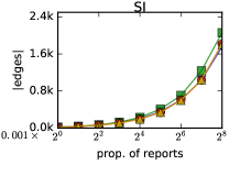
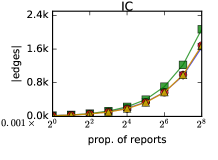
Figure 2: Tree size (objective function) produced by different methods in graph arxiv-hep-th, under si (left figure) and ic (right figure)

Precision and recall: We next demonstrate our methods’ adaptability on different graphs and models with respect to node precision and recall. Figure 3 varies the graphs while fixing the cascade model, meanwhile Figure 4 does the other way around.

In both Figure 3 and Figure 4, we observe that all four methods achieve node precision larger than 0.8. For most settings, node precision is close to 1. For ic model in Figure 4, precision drops slightly and delayed-bfs performs worse than the other three. Note that even though steiner does not explicitly cope with infection order, it still achieves equivalent performance. This demonstrates that the parsimony consideration in OrderedSteinerTree is reasonable with respect to achieving high node precision.

For node recall, we observe the following in both figures. First, arxiv-hep-th and grqc, node recall grows linearly as proportion of reports. However, for facebook and enron, node recall grows slower compared to the other two. The reason is facebook and enron are graphs with larger density, in which it generally takes fewer Steiner nodes to construct a Steiner tree.

Second, delayed-bfs tends to achieve higher recall than the other three because it does not explicitly minimize the tree size, therefore it captures more nodes. Third, closure, greedy and steiner tend to have similar recall.

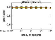
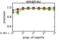
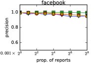
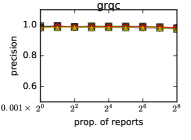
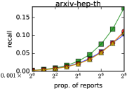
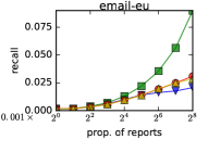
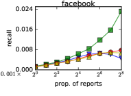
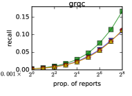
Figure 3: Node precision (upper row) and recall (lower row) for different graphs under si model.

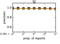
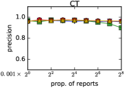
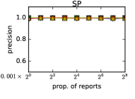
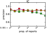
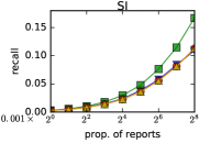
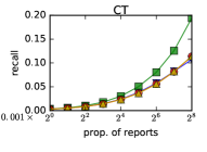
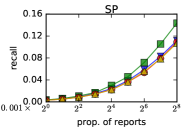
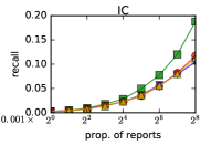
Figure 4: Node precision (upper row) and recall (lower row) for different models on grqc.

Order accuracy: Next, we report order accuracy. In general, closure, greedy and delayed-bfs perform better than steiner under all cascade models and all graphs. This advantage is demonstrated in Figure 5, in which the upper row fixes the cascade model while the lower row fixes the underlying graph. This is expected because closure and delayed-bfs explicitly construct tree that respect the infection order.

In addition, methods that models order explicitly improve their order accuracy as proportion of reports increase. However, this is not always true for steiner. For example, its order accuracy deteriorates for facebook and email-eu under ct in Figure 5.

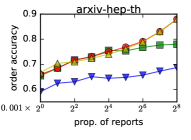
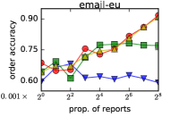
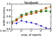
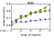
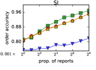
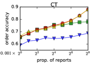
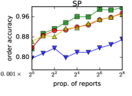
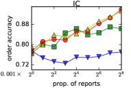
Figure 5: Order accuracy across datasets and cascade models. Upper row: under ct across all datasets. Lower row: in graph arxiv-hep-th under all models

Real cascades: Performance measure on real cascades is given in Figure 6 for both large and small cascades. For most the measures, they demonstrate similar behavior with respect to that on synthetic cascades. However, one noticeable difference is that node precision drops significantly. The reasons can be two-fold: 1) the infected nodes are tightly connected with each other as well as other uninfected nodes. In some cases, the uninfected nodes serve as good Steiner nodes 2) parsimony assumption does not hold for certain real cascades.

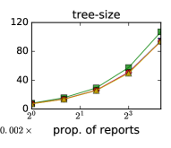
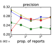
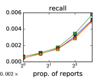
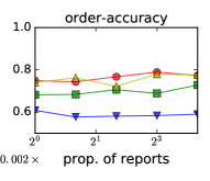
Figure 6: Performance measure on real cascades in Digg.

Scalability: Last, we evaluate the scalability of greedy. We conduct experiments on a 2.5 GHz Intel Xeon machine with 24 GB of memory.

First, we consider running time with respect to size of graphs (${\left|E\right|}$). We generate synthetic Barabási-Albert graphs with exponentially increasing sizes. Fraction of reports is fixed to 10%. The result is shown on the left-side of Figure 7. On the right side of the figure, we consider running time with respect to the fraction of reports on graph arxiv-hep-th. Both plots demonstrate greedy scales roughly linearly with respect to either ${\left|E\right|}$ or proportion of report.

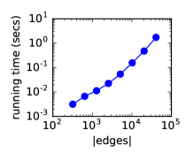
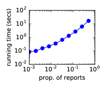
Figure 7: Running time greedy as a function of ${\left|E\right|}$ (left figure) and fraction of reports (right figure).

7 Conclusion

We introduce a new formulation for the cascade-reconstruction problem, based on a variant of the Steiner-tree problem—as it is common, the goal is to find a tree that spans all reported active nodes. The novelty of our approach is to effectively utilize temporal information of observations, namely, activation times. To account for the available temporal information we introduce temporal-consistency constraints, requiring that all paths in the discovered tree should preserve the order of the observed timestamps. For the proposed Steiner-tree problem we present three approximation algorithms, which provide a trade-off between quality guarantee and scalability. The most efficient algorithm has linearithmic running time, and thus, it is able to cope with very large graphs and large number of reported active nodes.

Our works opens interesting directions for future research. The main open problem is to close the gap between the approximation algorithms and inapproximability lower bounds. Another interesting direction is to consider a different objective function so as to improve the recall of the reconstructed cascade without significant harm on precision.

Acknowledgments. This work has been supported by the Academy of Finland projects “Nestor” (286211), “Agra” (313927), and “AIDA” (317085), and the EC H2020 RIA project “SoBigData” (654024).

A Proofs of statements related to the problem definition

Observation 2

The optimal solution to the OrderedSteinerTree problem is a tree rooted at the reported node $(u_{0},t_{0})\in R$. If there is more than one node in the set $V(t_{0})$, any of them can be considered as a root for the optimal tree.

• Assume a minimal Steiner tree $T$, rooted in some node $s$. Let $p$ be the path from $u_{0}$ to $s$. The reported nodes in $p$ have all timestamp equal to $t_{0}$. Let $v$ be a reported node, $q$ be a path from $v$ to $s$, and $q^{\prime}$ be the path from $v$ to $u_{0}$. Then $q^{\prime}$ contains a prefix of $q$ followed by (a part of) $p$. Since the reported nodes in $p$ have timestamp equal to $t_{0}$, it follows that $q^{\prime}$ is an order-respecting path. This allows us to re-root the tree from $s$ to $u_{0}$ while respecting the order.

Proposition A.1

Problem OrderedSteinerTree is NP-hard.

• The standard SteinerTree problem [17], with an input graph $G=(V,E)$ and a set of terminal nodes $X$, can be reduced to the OrderedSteinerTree problem with the same graph $G=(V,E)$ as the input and reported nodes $R=\{(x,0)\}$, for each $x\in X$.

B Approximation guarantee for closure

Proposition B.1

closure returns an order-respecting Steiner tree, which spans $R$.

• First, by the for-loop defined in lines 5–9, the resulting tree $T$ is a subgraph of $G$, which spans all reported nodes. For each new reported node $u$ processed in the for-loop, a new path $P$ is added in the subgraph $T$, which contains only one node from $T$, and thus $T$ is indeed a tree. Moreover, $P$ may contain only the largest time stamps in current $T$. This makes $T$ an order-respecting Steiner tree.

Proposition B.2

The closure algorithm provides approximation guarantee $2(1+\sqrt{3/2})\sqrt{k-1}$ for problem OrderedSteinerTree.

To prove this result we first need to prove couple of technical lemmas. Let us write $c=1+\sqrt{3/2}$ for brevity.

Lemma B.1

Assume a sequence of $n$ numbers. It is possible to partition this sequence in at most $c\sqrt{n}$ monotonic subsequences (increasing or decreasing).

Note that we are not referring to consecutive subsequences. For example, $(5,7,9)$ is a monotonically increasing subsequence of the sequence $(5,8,2,7,1,9,6)$.

• We will prove the lemma using induction on $n$. The result holds for $n=1,2,3,4$. Assume $n\geq 5$, and assume that lemma holds for any sequence of length less than $n$. Erdős-Szekeres theorem [21] states that there is a monotonic subsequence whose length is at least $\left\lfloor{\sqrt{n-1}}\right\rfloor+1$. By removing that monotonic subsequence we are left with a sequence having at most $n-\left\lfloor{\sqrt{n-1}}\right\rfloor-1$ numbers. By the induction hypothesis this reduced sequence can be partitioned in at most $c\sqrt{n-\left\lfloor{\sqrt{n-1}}\right\rfloor-1}$ monotonic subsequences. Thus, it is enough to prove that

  $$c\sqrt{n-\left\lfloor{\sqrt{n-1}}\right\rfloor-1}+1\leq c\sqrt{n}.$$

  To prove the claim note that

  $$\begin{split}0&=2c(c-2)-1\\ &\leq\sqrt{n-1}c(c-2)-1\\ &=c^{2}\sqrt{n-1}-2c\sqrt{n-1}-1\\ &\leq c^{2}\sqrt{n-1}-2c\sqrt{n-\sqrt{n-1}}-1\\ &=c^{2}n-c^{2}(n-\sqrt{n-1})-2c\sqrt{n-\sqrt{n-1}}-1\\ &=c^{2}n-\left(1+c\sqrt{n-\sqrt{n-1}}\right)^{2}.\end{split}$$

  That is,

  $$\left(1+c\sqrt{n-\sqrt{n-1}}\right)^{2}\leq c^{2}n,$$

  or

  $$c\sqrt{n-\sqrt{n-1}}+1\leq c\sqrt{n}.$$

  Since $\sqrt{n-1}\leq\left\lfloor{\sqrt{n-1}}\right\rfloor+1$, the lemma follows.

The next two lemmas show that there exists a directed tree in $H$ with total weight, say $w$, less than $2c\sqrt{k-1}$ times the number of edges in the solution. This immediately proves Proposition B.2 since that the total weight of the minimum spanning tree $A$ in closure is less or equal than $w$, and closure returns a tree with number of edges bounded by the total weight of $A$.

The first lemma establishes the bound when the reported nodes are leaves or a root, while the second lemma proves the general case when the reported nodes can be also internal nodes in the tree.

Lemma B.2

Let $G=(V,E)$ be a graph and let $R$ be a set of reported nodes. Consider a tree $T=(W,F)$, with $W\subseteq V$, whose root and leaves are exactly the reported nodes $V(R)$, with the root having the smallest timestamp. Then there is a directed tree $U=(V(R),B)$ such that $(u,v)\in B$ implies $t(u)\leq t(v)$, and

$$\sum_{(u,v)\in B}d(u,v)\leq 2c\sqrt{{\left|R\right|}-1}{\left|F\right|}.$$

• Write $k={\left|R\right|}$, and let $u_{1},\ldots,u_{k-1}$ be the leaves in $V(R)$, ordered based on a Eulerian tour. Let $s=u_{k}$ be the root of $T$. Consider any subsequence of $w_{1},\ldots,w_{\ell}$ of $u_{1},\ldots,u_{k-1}$. Then

  $$d(s,w_{1})+\sum_{i=1}^{\ell-1}d(w_{i},w_{i+1})\leq 2{\left|F\right|},$$

  since each $d(w_{i},w_{i+1})$ is upper-bounded by a path in the Euler tour and we visit every edge in ${\left|F\right|}$ at most twice during the tour. We can also reverse the direction of the tour and obtain

  $$d(s,w_{\ell})+\sum_{i=1}^{\ell-1}d(w_{i+1},w_{i})\leq 2{\left|F\right|}.$$

  To create the tree $U$, start with a tree containing only the root $s$. According to Lemma B.1 we can partition $u_{1},\ldots,u_{k-1}$ to at most $c\sqrt{k-1}$ sequences such that the timestamps of nodes in each subsequence is either increasing or decreasing. Let $w_{1},\ldots,w_{\ell}$ be such subsequence. If the time stamps are increasing, then add a path $s,w_{1},\ldots,w_{\ell}$. If the time stamps are decreasing, then add a path $s,w_{\ell},\ldots,w_{1}$. Repeat this at most $c\sqrt{k-1}$ times.

  The total distance weight of each path is $2{\left|F\right|}$ and there are at most $c\sqrt{k-1}$ paths, proving the result.

The second lemma allows reported nodes to be non-leaves.

Lemma B.3

Let $G=(V,E)$ be a graph and let $R$ be a set of reported nodes. Consider a tree $T=(W,F)$, with $W\subseteq V$, solving OrderedSteinerTree. Then there is a directed tree $U=(V(R),B)$ such that $(u,v)\in B$ implies $t(u)\leq t(v)$, and

$$\sum_{(u,v)\in B}d(u,v)\leq 2c\sqrt{{\left|R\right|}-1}{\left|F\right|}.$$

• We will prove this by induction over ${\left|V\right|}$. If there are no intermediate reported nodes in $T$, we can apply Lemma B.2 directly. Assume there is at least one, say $v$, intermediate reported node. Let $T_{1}$ be the tree corresponding to the branch rooted at $v$. Let $T_{2}$ be the tree obtained from $T$ by deleting $T_{1}$, but keeping $v$. Let $R_{1}$ be the reported nodes in $T_{2}$ and let $R_{2}$ be the reported nodes in $T_{2}$. Apply Lemma B.2 to $T_{1}$ and $T_{2}$, obtaining $U_{1}=(V(R_{1}),B_{1})$ and $U_{2}=(V(R_{2}),B_{2})$, respectively. We can join these two trees at $v$ to obtain a joint tree $U$. This tree respects the time constraints. Moreover,

  $$\begin{split}\sum_{(u,v)\in B}d(u,v)&=\sum_{(u,v)\in B_{1}}d(u,v)+\sum_{(u,v)\in B_{2}}d(u,v)\\ &\leq 2c\sqrt{{\left|R_{1}\right|}-1}{\left|F_{1}\right|}+2c\sqrt{{\left|R_{2}\right|}-1}{\left|F_{2}\right|}\\ &\leq 2c\sqrt{{\left|R\right|}-1}({\left|F_{1}\right|}+{\left|F_{2}\right|})\\ &=2c\sqrt{{\left|R\right|}-1}{\left|F\right|},\end{split}$$

  proving the result.

C Approximation guarantee of greedy

Proposition C.1

Algorithm greedy yields a $k$-approximation guarantee for the OrderedSteinerTree problem.

• Consider an input graph $G=(V,E)$, a set of reported nodes $R$, and seed $s$. Let $T^{*}$ be the optimal order-respecting tree that covers all reported nodes in $V(R)$, and $T$ be the tree returned by greedy. Let $c(T^{*})$ be the cost of optimal tree $T^{*}$, and $c(T)$ the cost of $T$. Let $p(s,u)$ be the shortest order-respecting path from $s$ to $u$ in $G$. For each reported node $u$ in $V(R)$ we have $c(p(s,u))\leq c(T^{*})$. In each iteration of greedy we add a path $Q^{+}(v,u)$ with $d^{+}(v,u)\leq c(p(s,u))$. It follows

  $$c(T)\leq\sum_{u\in V(R)}d^{+}(v,u)\leq\sum_{u\in V(R)}c(p(s,u))\leq k\,c(T^{*}).$$

D Approximation guarantee of delayed-bfs

Proposition D.1

Algorithm delayed-bfs yields a $k$-approximation guarantee for the OrderedSteinerTree problem.

• Let $T$ be the tree discovered by the algorithm delayed-bfs. We order the nodes in $V(R)$ based on the visiting by the algorithm, $V(R)=s_{1},\ldots,s_{k}$, We write $T_{i}$ for the (sub)tree that has been formed right after $s_{i}$ is added to the queue $Q$. We use $p_{i}$ to denote the depth of the tree $T_{i}$.

  Let $T^{*}$ be the optimal steiner tree, and let $T^{*}_{i}$ be a subtree of $T^{*}$ containing only branches with leaves from $s_{1},\ldots,s_{i}$.

  We claim that $p_{i}\leq{\left|E(T^{*}_{i})\right|}$. The proposition follows immediately from this claim since

  $${\left|E(T)\right|}\leq\sum_{i=1}^{k}p_{i}\leq\sum_{i=1}^{k}{\left|E(T^{*}_{i})\right|}\leq k{\left|E(T^{*})\right|}.$$

  To prove the claim, we use induction. The result holds trivially for $i=1$. Assume it holds for $i-1$. Let $j$ be the largest index such that $t(s_{j})<t(s_{i})$. If no index exist, then set $j=1$.

  Let $q$ be the length of the path in $T^{*}$ from $s_{i}$ to the largest ancestor terminal, say $s_{\ell}$, that is either a root or have a genuinely smaller time stamp.

  By induction $p_{j}\leq{\left|E(T^{*}_{j})\right|}$, and since $s_{\ell}\in V(T^{*}_{j})$, the tree $T_{j}$ can only grow by $q$ in depth before we visit $s_{i}$, that is, $p_{i}\leq p_{j}+q\leq{\left|E(T^{*}_{j})\right|}+q$. Note that $T^{*}_{j}$ does not contain the path from $s_{i}$ to $s_{\ell}$. This implies that ${\left|E(T^{*}_{j})\right|}+q\leq{\left|E(T^{*}_{i})\right|}$, proving the claim.

References

- [1] M. Gomez-Rodriguez, J. Leskovec, and B. Schölkopf, “Modeling information propagation with survival theory,” in Proceedings of the 30th International Conference on Machine Learning (ICML), 2013, pp. 666–674.
- [2] D. Kempe, J. Kleinberg, and É. Tardos, “Maximizing the spread of influence through a social network,” in Proceedings of the ninth ACM SIGKDD international conference on Knowledge discovery and data mining, 2003, pp. 137–146.
- [3] W. O. Kermack and A. G. McKendrick, “A contribution to the mathematical theory of epidemics,” in Proceedings of the Royal Society of London A: mathematical, physical and engineering sciences, vol. 115, no. 772. The Royal Society, 1927, pp. 700–721.
- [4] R. Pastor-Satorras and A. Vespignani, “Immunization of complex networks,” Physical Review E, vol. 65, no. 3, p. 036104, 2002.
- [5] B. A. Prakash, H. Tong, N. Valler, M. Faloutsos, and C. Faloutsos, “Virus propagation on time-varying networks: Theory and immunization algorithms,” in Joint European Conference on Machine Learning and Knowledge Discovery in Databases, 2010, pp. 99–114.
- [6] S. Feizi, K. Duffy, M. Kellis, and M. Medard, “Network infusion to infer information sources in networks,” in RECOMB, 2014.
- [7] M. Farajtabar, M. G. Rodriguez, M. Zamani, N. Du, H. Zha, and L. Song, “Back to the past: Source identification in diffusion networks from partially observed cascades,” in Artificial Intelligence and Statistics, 2015, pp. 232–240.
- [8] T. Lappas, E. Terzi, D. Gunopulos, and H. Mannila, “Finding effectors in social networks,” in Proceedings of the 16th ACM SIGKDD international conference on Knowledge discovery and data mining. ACM, 2010, pp. 1059–1068.
- [9] B. A. Prakash, J. Vreeken, and C. Faloutsos, “Spotting culprits in epidemics: How many and which ones?” in ICDM. IEEE, 2012.
- [10] P. Rozenshtein, A. Gionis, B. A. Prakash, and J. Vreeken, “Reconstructing an epidemic over time,” in Proceedings of the 22nd ACM SIGKDD International Conference on Knowledge Discovery and Data Mining. ACM, 2016, pp. 1835–1844.
- [11] E. Sadikov, M. Medina, J. Leskovec, and H. Garcia-Molina, “Correcting for missing data in information cascades,” in WSDM. ACM, 2011.
- [12] D. Shah and T. Zaman, “Rumors in a network: Who’s the culprit?” IEEE, vol. 57, no. 8, pp. 5163–5181, 2011.
- [13] S. Sundareisan, J. Vreeken, and B. A. Prakash, “Hidden hazards: Finding missing nodes in large graph epidemics,” in Proceedings of the 2015 SIAM International Conference on Data Mining. SIAM, 2015, pp. 415–423.
- [14] E. Sefer and C. Kingsford, “Diffusion archaeology for diffusion progression history reconstruction,” in ICDM, 2014, pp. 530–539.
- [15] M. Charikar, C. Chekuri, T.-y. Cheung, Z. Dai, A. Goel, S. Guha, and M. Li, “Approximation algorithms for directed steiner problems,” Journal of Algorithms, vol. 33, no. 1, pp. 73–91, 1999.
- [16] S. Huang, A. W.-C. Fu, and R. Liu, “Minimum spanning trees in temporal graphs,” in SIGMOD. ACM, 2015, pp. 419–430.
- [17] D. P. Williamson and D. B. Shmoys, The design of approximation algorithms. Cambridge university press, 2011.
- [18] M. X. Goemans and D. P. Williamson, “A general approximation technique for constrained forest problems,” in Proceedings of the Third Annual ACM-SIAM Symposium on Discrete Algorithms, ser. SODA ’92. Philadelphia, PA, USA: Society for Industrial and Applied Mathematics, 1992, pp. 307–316. [Online]. Available: http://dl.acm.org/citation.cfm?id=139404.139468
- [19] M. Gomez-Rodriguez, L. Song, N. Du, H. Zha, and B. Schölkopf, “Influence estimation and maximization in continuous-time diffusion networks,” ACM Trans. Inf. Syst., vol. 34, no. 2, pp. 9:1–9:33, Feb. 2016. [Online]. Available: http://doi.acm.org/10.1145/2824253
- [20] V. V. Vazirani, Approximation algorithms. Springer Science & Business Media, 2013.
- [21] P. Erdős and G. Szekeres, “A combinatorial problem in geometry,” Compositio Mathematica, vol. 2, pp. 463–470, 1935.