YITP-18-06
Conformal blocks from Wilson lines with loop corrections
Yasuaki Hikidaa***E-mail: yhikida@yukawa.kyoto-u.ac.jp and Takahiro Uetokob†††E-mail: rp0019fr@ed.ritsumei.ac.jp
aCenter for Gravitational Physics, Yukawa Institute for Theoretical Physics,
Kyoto University, Kyoto 606-8502, Japan
bDepartment of Physical Sciences, College of Science and Engineering,
Ritsumeikan University, Shiga 525-8577, Japan
We compute the conformal blocks of the Virasoro minimal model or its WN extension with large central charge from Wilson line networks in a Chern-Simons theory including loop corrections. In our previous work, we offered a prescription to regularize divergences from loops attached to Wilson lines. In this paper, we generalize our method with the prescription by dealing with more general operators for and apply it to the identity W3 block. We further compute general light-light blocks and heavy-light correlators for with the Wilson line method and compare the results with known ones obtained using a different prescription. We briefly discuss general W3 blocks.
1 Introduction
Two dimensional conformal field theory (CFT) with large central charge is supposed to be dual to the semi-classical regime of three dimensional gravity on anti-de Sitter (AdS) space. Since holography is expected to provide a formulation of quantum gravity in terms of dual CFT, we would obtain some insights on the quantum aspects of gravity from corrections in dual CFT. As a simple example, we examine the WN minimal model, which has a coset description as
| (1.1) |
with the central charge
| (1.2) |
The dual bulk description was proposed to be the Chern-Simons gauge theory based on Lie algebra [1]. In particular, we can study the quantum corrections of AdS3 gravity in terms of the Virasoro minimal model given by the coset (1.1) with . We consider the large regime of the minimal model, which corresponds to a perturbative regime of Chern-Simons theory. The expression of central charge (1.2) implies that ; thus, the large regime of the model should be non-unitary. Nevertheless, the holography has been argued to work [2, 3, 4], and it should be useful at least for problems related to its symmetry algebra.
The basic quantities of CFT are the spectrum of operators and correlation functions or conformal blocks. In particular, the conformal block decomposition of the correlator is an essential tool for recent developments on conformal bootstrap programs (see, e.g., [5]). In terms of Chern-Simons theory, conformal blocks at the large limit were proposed to be computed by the networks of open Wilson lines, and the proposal was confirmed for explicit examples [6, 7]. In this paper, we develop techniques to evaluate conformal blocks beyond the large limit by applying recent works on loop effects for Wilson lines in [8, 9, 10], see also [11]. The proposal of the map between conformal blocks and Wilson line networks in [6, 7] can be easily extended beyond the large limit as in [9]. We evaluate the corrections of conformal blocks from the loop corrections of the Wilson line networks. The computations are rather subtle, and a main issue is how to regularize divergences associated with loop diagrams. In the language of the usual Lagrangian formulation, how to deal with this kind of divergences was established. Since we are dealing with open Wilson lines instead of Lagrangian, it is quite non-trivial to formulate a general procedure. In our previous paper [10], we offered a way to regularize divergences by renormalizing parameters in Wilson lines, which correspond to couplings between bulk scalars and a higher spin current, along with rescaling the overall factor of open Wilson lines. Moreover, we showed that ambiguities related to the renormalization procedure can be removed by requiring that the correlators of boundary theory are consistent with the symmetry. In this paper, we adopt the renormalization procedure in [10] for regularizing divergences.
The primary operators of the WN minimal model (1.1) are labeled as , where represent the highest weights of su Lie algebra. The operator with (where f denotes the fundamental representation of su) is dual to a bulk scalar field, and the operators with correspond to their composite fields [1]. On the other hand, the operator with has its conformal weight of order , and it is proposed to be dual to a conical defect geometry [2, 3, 4]. The symmetry of WN algebra for the model (1.1) is generated by higher spin currents with . In [10], we evaluated the correlators as
| (1.3) |
with general (where represents the spin of representation) for and with for . In particular, we reproduced the corrections of conformal weight for operators dual to bulk scalars up to order by adopting our regularization prescription.111For , the conformal weight of operator was reproduced up to order in [9] by applying a Wilson line method, which is possible without specifying any regularization prescription.
In this paper, we extend the previous analysis and apply our Wilson line method to four point conformal blocks with and . For , we consider the correlator as
| (1.4) |
with . The conformal blocks were already examined by utilizing open Wilson lines in [8]. Since we adopt a different regularization prescription, our formulation is not the same as theirs. We can easily relate the two methods for the identity Virasoro block, so we focus on general Virasoro blocks.222We refer to the conformal block with the identity operator or its descendants exchanged as an identity block and to other conformal blocks as general blocks. In [8], they obtained the all-order expression in for the general Virasoro block up to order except for the -independent part. For the part, they obtained the first few terms in expansion. We compute the general block with our formulation and obtain the all-order expression in up to order including the -independent part. For , we examine the four point conformal block (1.4) with setting for simplicity. We explicitly compute the identity W3 block using the product of two open Wilson lines and reproduce the CFT result. For the purpose we first extend the previous analysis for the two and three point functions (1.3) by dealing with general for . The general W3 blocks at the leading order in were obtained in [12] from the CFT viewpoint, and they were reproduced in [7] using the networks of the open Wilson line. We point out that our formulation combines these results in a quite nice way. We also analyze the correction of a simple non-identity W3 block with .
We further consider the four point function with heavy operators as
| (1.5) |
with . The heavy operator corresponds to a conical defect geometry as mentioned above, and we compute the correlator using an open Wilson line in the conical space. For quantum corrections to the open Wilson line, we adopt our formulation developed so far. For quantum corrections to the conical geometry, we make use of the results in [13] obtained by applying the coadjoint orbits of the Virasoro group in [14, 15]. In this way, we reproduce the previous results from CFT computation in [16, 17, 18]. The Wilson line method was used in [7, 8] at the leading order in , where they used open Wilson lines for the heavy operators instead of conical spaces. For general , the computation with our method reduces to those in [19, 20] at the leading order in .
The organization of this paper is as follows. In the next section, we introduce the WN minimal model and write down the expressions of conformal blocks examined in terms of Wilson lines in this paper. In section 3, we explain our bulk method for conformal blocks particularly focusing on our prescription for regularizing divergences. In subsection 3.2, we review our previous work in [10] on the two and three point functions (1.3) for , and in subsection 3.3, we extend the analysis by considering general light operators with . In section 4, we apply the method to compute conformal blocks from the bulk viewpoint. In subsection 4.1, we obtain the identity W3 block from the product of two Wilson lines and compare it to the CFT result. In subsection 4.2, we examine general Virasoro blocks with our formulation and see the relation to previous results in [8]. We further discuss general W3 blocks. In section 5, we apply our formulation to correlators with two heavy operators along with two light operators for . We conclude this paper and discuss open problems in section 6. In appendix A, we summarize CFT computations of four point conformal blocks in the WN minimal model. In particular, we obtain four point function of (1.4) with corresponding a rectangular Young diagram and . As an application of [21, 10], we compute the corrections of higher spin charges for the scalar operators using the method of conformal block decomposition. In appendix B, we include some technical details of sl Lie algebras. In appendix C, we compute the correction of a simple non-identity W3 block. In appendix D, we examine how correlators obtained from Wilson lines change under local conformal transformations.
2 WN minimal model
The minimal model of WN algebra can be described by the coset (1.1) with the central charge (1.2), see, e.g., [22, 23, 24] for some details. The primary states are labeled as with as the highest weights of su Lie algebra. We denote as the numbers of boxes in the -th row of Young diagrams corresponding to and define power sums as
| (2.1) |
by following [4]. Here, denote the numbers of boxes in , and are given by
| (2.2) |
The components of the Weyl vector are The conformal weight of primary state is then written as
| (2.3) |
The two point function of the operator is fixed by the symmetry as
| (2.4) |
The overall normalization can be set arbitrary by changing the definition of operator. Here and in the following, we only consider the holomorphic sector, but it is straightforward to include the anti-holomorphic sector.
We are interested in a regime with the large central charge (1.2) but finite , which implies that we should take
| (2.5) |
In the regime, the conformal weight behaves as for while for . For a while, we focus on the case only with light operators , and later, we examine correlators with as well. For , we label the representation of su(2) by spin quantum number , where is defined above. The conformal weight of the operator with is given by
| (2.6) |
in expansion. For general , we expand the highest weight in the fundamental weights as , where are the Dynkin labels. As a simple but non-trivial example, we also study in some details the case, where the Dynkin labels are related as and . The conformal weight of the operator with is
| (2.7) |
For general , the computation of correlators is simplified when , which corresponds to the case with , . The conformal weight of the operator with is
| (2.8) |
Expanding the conformal weight (2.3) in as
| (2.9) |
the two point function (2.4) becomes
| (2.10) |
Later we shall see that the bulk computations reproduce the shifts of conformal weight from the terms proportional to .
The symmetry of WN algebra is generated by higher spin currents with . In this paper, we adopt the convention for the higher spin currents in [21, 10]. In particular, the two point functions are given by
| (2.11) |
with
| (2.12) |
For , we have
| (2.13) |
and, in particular, the normalization for the spin 2 current is the same as the usual one for the energy momentum tensor, i.e., . The three point function with a higher spin current is fixed by the Ward identity as
| (2.14) |
where denotes the spin charge of the operator . The spin 2 charge is nothing but the conformal weight as in (2.3). The expression of spin 3 charge may be found in [25, 2, 4] as
| (2.15) |
where the overall factor is due to our convention for the spin 3 current. For , the spin 3 charge of the operator is given by
| (2.16) |
For general , the spin 3 charge of the operator is
| (2.17) |
in expansion.
A main aim of this paper is to examine conformal blocks using open Wilson lines in the bulk theory. For , we consider the four point function of scalar operators in (1.4) with , that is
| (2.18) |
Here we have used since the finite representation of su(2) is self-conjugate. The identity Virasoro block has been evaluated using Wilson lines up to order as [8]
| (2.19) |
where the expressions of may be used as in (A.11) of [21]. Here, at the order corresponds to the global block333The global part of Virasoro algebra is given by sl(2) algebra, and only the sl(2) descendants are considered as intermediate states for the global block. with the exchange of the energy momentum tensor. We do not compute the identity block with the Wilson line method since there is no significant difference from the previous computation in [8]. The Virasoro block with the intermediate operator was similarly obtained up to order as
| (2.20) |
All order expressions in for and and the first few orders in for were obtained in [8]. In subsection 4.2, we examine the general block, applying our method, and, in particular, we obtain all order expressions in even for .
For correlators in the WN minimal model with general , we may compute correlators by applying the Coulomb gas method as explained in appendix A, see, e.g., [26, 27, 28, 29, 19]. A conformal block is given by a choice of integration contour over the positions of screening operators inserted. Since it is non-trivial to identify proper integration contours,444We are particularly interested in the identity WN block, which appears in the -channel decomposition of the four point function (1.4). However, we cannot find out any references giving the -channel expressions. The expressions in the -channel or the -channel were obtained in [26, 27] when or correspond to a degenerate representation, see also [29]. we consider the simple correlator
| (2.21) |
In this case, the Coulomb integrals reduce to a hypergeometric function , and we can apply the analysis for the Virasoro minimal model, see, e.g., [30]. The final result obtained in appendix A is
| (2.22) | |||
with
| (2.23) |
The first and second terms correspond to the WN blocks of identity and adjoint operators, respectively. In subsection 4.1, we examine the identity W3 block up to the order. In subsection 4.2.3, we give some comments on general W3 blocks, and in appendix C, we analyze the adjoint W3 block with up to the order.
The identity WN block is a useful quantity even in the CFT perspective. For instance, we proposed a way to obtain the correction of spin charge for the primary operator in the WN minimal model (1.1) by utilizing the Virasoro block decomposition of the identity WN block in [21, 10]. Since the WN minimal model is a solvable model, we know how to obtain the higher spin charges with finite as in [22, 31, 32]. However, in practice, it is difficult to obtain their explicit expressions for larger , and our method provides a simple way to obtain them including corrections. In [21, 10], we have considered higher spin charges for operators only in the fundamental representation. In appendix A, we extend the analysis by examining higher spin charges for the operator with including corrections.555See [33] for a recent work on higher spin charges for general operators in a supersymmetric model. Among others, we can reproduce the correction of spin 3 charge in (2.17).
We also apply our approach to heavy-light correlators. At the leading order in , general CFT correlators of this type were reproduced from the analysis of the open Wilson line in a conical space in [19, 20]. For the analysis of corrections, we may work on a simple form of the correlator as
| (2.24) |
In this case, there is only one type of exchanged operator, and the Coulomb integrals can be carried out as (see, e.g., [19])
| (2.25) |
We reproduce the CFT result for by applying our method for open Wilson lines and the analysis for conical spaces in [13]. The bulk approach should be applicable also for general , but we leave detailed analysis to future work.
3 Method for bulk computation
In this section, we explain our method to compute correlators or conformal blocks from the networks of open Wilson lines. In the next subsection, we first introduce Chern-Simons gauge theory and the networks of Wilson lines corresponding to conformal blocks. We then explain our prescription developed in [10] to remove divergences associated with loop diagrams. In subsection 3.2, we review our previous work in [10] on the two point function of a scalar operator and the three point function with two scalars and a spin 2 current for . The analysis can be extended straightforwardly for if the scalar operator belongs to the (anti-)fundamental representation of su(3). In subsection 3.3, we extend our method by analyzing correlators involving general scalar operators.
3.1 Chern-Simons theory and open Wilson lines
The bulk description of the WN minimal model with large was proposed to be given by Chern-Simons gauge theory [2], the action of which is
| (3.1) |
Here, is the level of the Chern-Simons theory, and takes values in sl Lie algebra.666We neglect throughout this paper, but can be analyzed similarly. As a higher spin gravity, it is important to decompose the generators of sl Lie algebra in terms of embedded sl. We consider the principal embedding as
| (3.2) |
Here, denotes the -dimensional representation of sl, which is generated by . A solution to the equations of motion can be written in a form as
| (3.3) |
by fixing a gauge. Here, denotes the radial coordinate, and the boundary is located at . Moreover, are coordinates parallel to the boundary. With the coordinates, the AdS metric is given by , and the corresponding configuration of the gauge field is with . As for the application to AdS gravity, we assign the asymptotic AdS condition, which restricts the from of the gauge field as [34, 35, 36, 37]
| (3.4) |
with in (2.12). The asymptotic symmetry near the AdS boundary is identified as the WN algebra generated by . The central charge of the algebra is
| (3.5) |
at the classical level, which is same as for the pure gravity in [38]. With the coefficients of in (3.4), the normalization of currents is the same as that in (2.11) at the leading order in .
We would like to compute the correlators or conformal blocks of the WN minimal model in terms of Wilson line operator
| (3.6) |
in the sl Chern-Simons theory. Here we remove the -dependence by a gauge transformation as . At the leading order in , it has been argued that -point conformal blocks can be evaluated as [6, 7, 9]
| (3.7) |
where denotes the highest weight state in the representation of sl. Moreover, belongs to a singlet representation in . There are several ways to construct a singlet state, and a choice of singlet leads to one of conformal blocks, see [7] for more explanations and explicit examples. The open Wilson lines are connected at a point , but the expression should be independent of . For , we may set ,777If we instead set , then we obtain with and in the representations and , respectively. then, the expression of (3.7) becomes
| (3.8) |
Here represents the lowest weight state in the representation , which is the conjugate of .
For evaluating quantum effects in the Wilson line network (3.7), we should integrate over gauge fields in the path integral with the insertions of Wilson line operators. Following [8, 9, 10], we evaluate the expectation values by using the correlators of in (3.6) with (3.4) in terms of the theory with WN symmetry as in (2.11). Here the normalization (2.12) is set in terms of the central charge , so it is regarded as the full propagator after including loop corrections, see [9] for the arguments. We also need to integrate over along the Wilson line in (3.6). However, the integration would diverge when at least two of collide at the same point. As in [10], we introduce a regular and replace (2.11) by
| (3.9) |
A merit of this choice is that the regulator does not break the scale invariance. The integration over would diverge when , and we remove the divergence by renormalizing the overall normalization of Wilson lines and parameters corresponding to interactions as in [10]. We denote the parameters as
| (3.10) |
and insert them into the Wilson line operator as
| (3.11) |
We can remove some divergences at the order by using and similarly for higher orders. There are still ambiguities for the terms of order , and we offer to fix them such that the boundary correlators are consistent with the WN symmetry.
3.2 Two and three point functions for
In order to illustrate our method and fix notations, we review our analysis in [10] for the two and three point functions in (1.3). For , it is convenient to work with the -basis, which can be applied to the general case but with operators in the (anti-) fundamental representation. As in [39, 8, 10], we consider the -basis expression of (3.8) as
| (3.12) |
For brevity, we call the left hand side . With the basis, we can use
| (3.13) |
where for and for general . The generators are [40]
| (3.14) |
and, in particular, the sl subalgebra is generated by
| (3.15) |
As in [8, 9, 10], we express (3.12) as
| (3.16) |
with
| (3.17) | |||
in expansion.
Let us first evaluate the two point function of operator for as
| (3.18) |
with by applying our Wilson line method. At the leading order in , the two point function becomes
| (3.19) |
as expected. The contribution at the next order is
| (3.20) |
where we have used (3.9). We can remove the term proportional to by changing the overall normalization of Wilson line operator. The shift of conformal weight can be read off from the term proportional to as in (2.10), and the order term in (2.6) is successfully reproduced.
We also examine a three point function using Wilson line operator as
| (3.21) |
with the extra insertion of the spin 2 current. At the leading order in , we have
| (3.22) |
as in (2.14). At the next leading order, there are two types of contributions as
| (3.23) | |||
We use the correlators
| (3.24) |
for the three point function and
| (3.25) |
with up to order for the four point function. The sum of the integrals leads to
| (3.26) |
We remove the divergence by renormalizing the coupling in (3.11) as (see (4.21) of [10])
| (3.27) |
Here the constant term is chosen such that the three point function becomes
| (3.28) |
with in (2.6) up to order . In other words, we chose the renormalization scheme to be consistent with the conformal Ward identity in the boundary theory. Here, we remark that the renormalized coupling in (3.27) is independent of ; thus, the same Wilson line operator (3.11) can be used to evaluate the network in (3.7).
In [10], we also examined the order corrections of the two point function, and we reproduced the shift of conformal weight at the order as in (2.6). This is possible only after properly regularizing divergences and this fact gives a support for our renormalization prescription, see [10] for more details. The analysis here can be directly applied to the case with but involving scalar operators only in the (anti-)fundamental representation. Similarly for , we showed in [10] that the divergences at the order in the two and three point functions of the form (1.3) can be removed by renormalizing the overall factor of Wilson line operator and couplings and introduced as in (3.11). With the renormalization at the order, we reproduced the shift of conformal weight of scalar operator up to the order.
3.3 Two and three point functions for
In [10], we restrict ourselves to operators only in the (anti-)fundamental representation. However, the fusion of this type of operators would yield another operator belonging to a representation other than the (anti-)fundamental one. Therefore, it is necessary to extend the previous analysis and deal with correlators involving general operators. It is known that sl generators acting on general states can be represented by using parameters with the number of the positive root. For , we introduce three parameters , which makes the expression (3.16) with (3.17) applicable to the general situation. The explicit expressions of states and generators are summarized in appendix B.
Just like the case, we start from computing the two point function of operator using the Wilson line as
| (3.29) |
The expression of the Wilson line in expansions in (3.16) with (3.17) leads to
| (3.30) |
with the normalization of (B.3). This is consistent with the leading order expression of conformal weight in (2.7). At the next leading order in , we have the contributions as
| (3.31) |
where are given by (3.17) with (B.7), (B.9), and (B.10). Moreover, we use the two point functions of currents in (3.9) with
| (3.32) |
see (2.13) with . The sum of the both contributions is
| (3.33) |
up to the orders of and . The -independent overall factor can be set as by changing the normalization of the Wilson line operator. From the coefficient of , the shift of conformal dimension can be read off as
| (3.34) |
which reproduces the order term in (2.7).
Next we move to the evaluation of Wilson line operator with the insertion of a higher spin current with or . We would like to show that the three point functions can be reproduced as
| (3.35) |
Let us define
| (3.36) |
with . We first examine the leading order in . From the expression of the open Wilson line in (3.16) with (3.17), we find
| (3.37) |
using (B.7), (B.9), and (B.10). There are no divergences from these tree level computations, which reproduce (2.14) with (2.7) and (2.16) at this order.
Divergences arise from the next order in . For in (3.36) at this order, a type of contributions comes from the integrals as888We take the limit for these computations.
| (3.38) |
Here, we have used the three point functions (3.24) and
| (3.39) |
where the powers are obtained by shifting the conformal weights of and as and , respectively. Another type is
| (3.40) |
with . Here the large factorization of four point functions is used as (3.25) and
| (3.41) |
Totally, we have
| (3.42) |
up to orders and . There is a divergent term proportional to , which is removed by shifting the coupling introduced in (3.11) from its classical value . We choose the -independent part of as
| (3.43) |
then we reproduce the CFT result in (2.14) with (2.7) as
| (3.44) |
up to the order . Note that the shift of coupling in (3.43) is the same as (5.17) of [10], and it is independent of the representation .
We can similarly analyze in (3.36). At the order, contributions are
| (3.45) |
and
| (3.46) |
with . Here we have used (3.39), (3.25), and (3.41). The sum of them leads to
| (3.47) |
up to orders and . Changing the coupling in (3.11) as (see (5.30) of [10])
| (3.48) |
the above expression becomes
| (3.49) |
up to the order as in (2.14) with (2.16). Here, we remark that the shift of is independent of as for .
Adopting the regularization, we should be able to reproduce the shift of conformal weight up to order just like the case with in [10]. Here we do not repeat the computation since it is not necessary for the following analysis.
4 Conformal blocks from open Wilson lines
In this section, we evaluate four point conformal blocks of the form (1.4) by including quantum effects on the networks of open Wilson lines. For , similar computations were done in [8], but their formulation is different from ours. In the next subsection we start from the identity blocks, which are computable by the products of two open Wilson lines. Since computations turn out to be quite similar to those in [8] for , we focus on the case by applying the method developed in the previous section. In subsection 4.2, we examine general conformal blocks, where we have to really deal with the networks of open Wilson lines. We concentrate on the simpler case with and briefly discuss the extensions, see also appendix C.
4.1 Identity W3 blocks
In order to express a conformal block for (1.4) in terms of the Wilson line network as in (3.7), we have to choose a proper singlet from the product of representations as explained in subsection 3.1. For the identity block, we set as the direct product of two singlets given by and . With the choice, the Wilson line network factorizes as
| (4.1) |
with . Setting and with and , the Wilson line network becomes the product of two open Wilson lines. Therefore, the identity block should be computed as
| (4.2) |
where the products of currents are evaluated by the correlators of WN theory as before. In this subsection we explicitly compute (4.2) for with and , that is
| (4.3) |
by applying the method developed in the previous section. We compare the result with the identity block from the CFT computation in (2.22), see appendix A for some details. The expansion is given as (A.28) with (A.29), but now we set and .
The leading order expression in is simply given by the product of two expectation values as
| (4.4) |
This can be expressed in diagram (a) of figure 1.
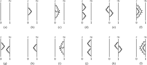
Among higher order corrections in , there are contributions of the self-energy type as in other diagrams. For contributions corresponding to diagrams (b)-(f), we replace in (4.4) the integrals of the forms
| (4.5) |
with and . Here, the integrals with and correspond to diagrams (b) and (c). The integrals with include the four point functions of currents with several different terms as in (3.25) and (3.41), which are expressed by diagrams (d), (e), and (f). The corrections to up to order have been evaluated in [10], and they can be summarized as the shift of conformal dimension from (4.4) to (see (2.7) for a general operator)
| (4.6) |
after renormalizing the overall factor of the open Wilson line and the coupling constants in (3.11). The other diagrams correspond to the similar corrections of another Wilson line , but they do not appear in the four point block (4.3) since an operator is put at the infinity.
Non-trivial contributions start to enter from the next order in . They correspond to diagram (a) of figure 2,
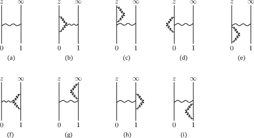
and the sum of them is
| (4.7) |
with
| (4.8) |
With the two point functions of currents in (2.11) with (3.32), we evaluate the integrals as
| (4.9) |
They correspond to the global blocks with spin 2 and 3 currents as the intermediate operators as they should be. The coefficients are also given by the products of three point functions divided by a current-current two point function as
| (4.10) |
at the leading order in . Here, the spin 2 and 3 charges were given by (2.7) and (2.16).
The other diagrams in figure 2 yield loop corrections to interactions among an open Wilson line and an exchanged current. These diagrams can be evaluated precisely as for (3.36) but with replaced by or . Therefore, after renormalizing the open Wilson lines and the coupling constants , the net effects are summarized as the order terms in (2.7) and (2.16) as
| (4.11) |
Thus we have a type of corrections as
| (4.12) |
coming from diagrams (b)-(i) of figure 2.
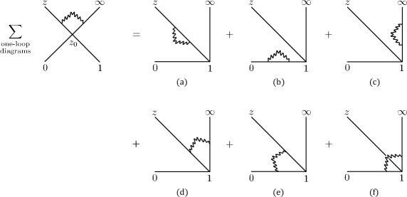
At the order of , there are more interesting contributions with the exchange of two currents as in diagrams (a) and (b) of figure 3 in addition to those already given. When the two currents have the same spin, they come from the integrals
| (4.13) |
with . The first and second terms are expressed by diagrams (a) and (b), respectively. When the two currents have the different spins, the contributions corresponding to diagrams (a) and (b) are given by the integrals
| (4.14) |
with or .

Summing over this type of contributions, we find
| (4.15) | |||
with . The total contribution at the order other than the self-energy type is thus
| (4.16) |
We confirm the bulk computation by showing that the above result reproduces the CFT one. The identity block in (2.22) is expanded in as (A.28) with (A.29), and we set , and identify for the comparison. We can see that the order term in (A.28) is the same as (4.7) with (4.9). Furthermore. we can check that the order expression of (A.28) with (A.29) is reproduced by (4.16) at each order in expansion.
Before ending this subsection, we would like to mention the relation to the analysis in [8] for with a different regularization. The regularization prescription in [8] is to adopt the normal ordered product for currents coming from the same Wilson line operator. Moreover, they used the exact conformal weight from the beginning instead of the quantum number for the finite representation of sl. Using the normal ordered prescription is equivalent to neglecting contributions coming from loop diagrams in figures 1 and 2, see also [9]. As we explained above, these contributions only shift the conformal weight for ; therefore, the effect is already included in their treatment. The contributions represented by diagrams in figure 3 are the same in the both prescriptions, see figure 5 of [8]. Therefore, we can see that the both ways of computation should give the same result for .
4.2 General conformal blocks
In this subsection, we study the conformal blocks with the exchange of the general operator from the networks of open Wilson lines (3.7) by including quantum effects. For the general blocks, it turns out to be convenient to use the -basis as
| (4.17) |
in its conjugated form. Here the generators are now written in terms of as explicitly indicated in the arguments of the Wilson line operator. The condition for the singlet becomes
| (4.18) |
for all and . In general there are several solutions, and a solution corresponds to a conformal block. Applying as in (3.13) or (B.2), the expression is simplified as
| (4.19) |
The quantum effects are evaluated by using the correlators of higher spin currents inserted as before.
In the following we mainly focus on the case and make some comments on the case at the end of this subsection. Before going into the details on three and four point Virasoro blocks, let us mention how the formalism explained above reproduces the previous analysis on the two point function for . We examine in (4.19) with . The vertex is given by the unique solution to the singlet condition (4.18) as (see, e.g., [12])
| (4.20) |
up to the overall factor. At the leading order in , we have
| (4.21) |
as in (3.19). For the corrections, it is convenient to set (or ), which reduces the number of diagrams, see figure 4.

With , the expression in (4.19) reduces to the expectation value of (3.12) with (3.13) and . We have also evaluated the corrections to the two point function with keeping generic and checked that the final result is the same.
4.2.1 Three point Virasoro block
As a simple but non-trivial example, we study three point conformal block for . The three point block is fixed by the conformal symmetry as
| (4.22) |
with (see (2.6))
| (4.23) |
We evaluate in (4.19) with . The vertex is uniquely fixed by the singlet condition (4.18) as (see, e.g., [12, 8])
| (4.24) |
up to the overall factor. At the leading order in , we find
| (4.25) |
The expression reproduces the three point function at the leading order in . Here we simply replace by ,999Precisely speaking, are replaced by with as the position of vertex for the Wilson line network. Since the results do not depend on , we can set . and this is actually as the same as the prescription to obtain the large limit of three point Virasoro block in [12].
We move to the next leading order in . When evaluating the expectation value of , the correlators of for Virasoro algebra are used, and divergences are removed as before. In order to make the computation simpler, we set . Moreover, using ,101010Similarly to the two point function, we have checked that the final result in (4.27) does not depend on even for generic . For more complicated correlators, the computations would be quite messy without setting as a specific value. we consider the product of two Wilson lines as in figure 5.

With this setup, we evaluate the integrals corresponding to the three diagrams in the right hand side. Defining
| (4.26) | |||
the integrals corresponding to diagrams (a), (b), and (c) are with , respectively. The order correction to the three point conformal block is given by the sum of them as
| (4.27) |
with in (4.23) up to the order term. Here we have ignored the term proportional to the tree level expression, which is interpreted as a correction to the overall factor of three point function. The result reproduces the order correction of three point block in (4.22) with (4.23) by setting .
4.2.2 Four point Virasoro block
We move to the Virasoro block of operator for the four point function (2.18). For this correlator, we may set and . We compute in (4.19) with . A solution to the singlet condition (4.18) is given by [12]
| (4.28) |
where we have defined
| (4.29) |
With the integral contour as and the overall factor as
| (4.30) |
the leading order expression in becomes
| (4.31) |
where is the global block of operator as
| (4.32) |
Just like the three point block, this is essentially the way to obtain the large limit of the four point block in [12].
For the next leading order in , we evaluate the network of open Wilson lines with . With this setting, the number of diagrams we have to consider is reduced as in figure 6.
We choose the normalization of conformal block as
| (4.33) |
and hence we subtract the terms proportional to the global block (4.32) such that there is no term at the order. With defined in (4.26), the integrals corresponding to diagrams (a), (b), and (e) are written as
| (4.34) |
with , respectively. For other diagrams, we define the functions as
| (4.35) |
with , and
| (4.36) |
with . Then the integrals corresponding to diagrams (d) and (f) are
| (4.37) |
respectively. The sum of all contributions is computed as
| (4.38) |
up to the terms proportional to (4.32). Here we neglected the integral corresponding to diagram (c) since it can be shown to give only terms proportional to (4.32) or with .
Let us compare the order expression with the known result in (2.20). First we examine the term in (4.38). This type of contribution comes from the shifts of conformal weights as
| (4.39) |
with
| (4.40) |
We can see that the term proportional to successfully reproduces the corresponding term in (4.38). There is another type of contribution summarized as
| (4.41) |
We read off the functions from (4.38) as
| (4.42) |
The functions reproduce those in [8]. For the other function , the terms proportional to were obtained in [8], and the -expansion of the above result correctly reproduces them. In other words, our method enables us to obtain the all-order expression in at the next non-trivial order in , which was not available before.
One may wonder how this becomes possible. In [8], the authors evaluated the operator product expansion (OPE) blocks in the sense of [41] in terms of open Wilson lines and then computed the four point Virasoro blocks using the expression of the OPE blocks. The procedure requires the integration over for the two point function of the intermediate state as , while we need to integrate over only one parameter except for the positions of the currents inserted. We think that this is a main reason for the simplicity.
4.2.3 General W3 blocks
So far we have analyzed general Virasoro blocks, but we also would like to make some comments on general W3 blocks. We are interested in the expectation value of in (4.19), where we can obtain the vertex of open Wilson lines by solving the singlet condition in (4.18). Solutions to the condition were obtained in [12] for , which may be denoted as
| (4.43) |
for the -point function. For , the representation of an external operator is restricted to be degenerated as or . A solution for is written as an integral of the product of two solutions, so there are also similar restrictions on the representations of external operators.
We first indicate that our formulation reduces to the one in [12] at the leading order in . At this order, the expression in (4.19) reduces to
| (4.44) |
where we have set by using the independence of . Utilizing the formula (B.8), we can see that the leading order expression is obtained from by replacing with . Just like the case, the recipe to obtain the large limit of the W3 block is the same as the one in [12]. As a result of this fact, we can conclude that our formulation with Wilson lines reproduces the large limit of W3 blocks as obtained in [12], see also [42]. Similar analysis with Wilson lines was done in [7] with a different technique for algebraic calculations. Our method with the -basis makes computations easier for generic representations as seen above, but their method seems to be convenient for a simple representation, such as, . In appendix C, we compute the correction of a simple non-identity W3 block from the Wilson line network (3.7) by utilizing their analysis.
We can also show that the analysis of two point function reduces to the previous one in subsection 3.3. For , the solution to the singlet condition (4.18) was obtained in [12] as
| (4.45) |
For , the expression in (4.19) becomes
| (4.46) |
as for (3.16) with (3.17). Here, we have used
| (4.47) |
where was defined in (B.3) with . Similarly, for , we obtain
| (4.48) |
but now is with .
5 Heavy-light correlator
The WN minimal model includes light operators of order and heavy operators of order as explained in section 2. Heavy operators correspond to non-trivial geometries, and correlators with heavy operators are important for examining their quantum effects. In this section, we examine a heavy-light correlator for the simplest case with , and in section 6, we make some comments on the general cases with .
For the analysis in this section, it is convenient to adopt the usual convention for the label of primary operators by two positive integers , see [30] for a review. In section 2, we have used the numbers of boxes in Young diagrams as and the relation is . The conformal weight of primary operator is given by (2.3) as
| (5.1) |
which is of order for . We study the four point correlator in (2.24) with , for , the expression with finite of which can be found in (2.25).
It is also useful to work on the cylindrical coordinate , which is related to the planar one as . In particular, the conformal weight is shifted from in (5.1) to . The expression of the four point function in (2.25) becomes111111We have changed the phase factor for convenience, but it does not matter when we consider the product with the anti-holomorphic sector.
| (5.2) |
in the expansion. In the rest of this section, we shall reproduce it from the bulk viewpoint.
5.1 Conical spaces in AdS3 gravity
As explained in section 2, and are supposed to be dual to a conical geometry and a bulk scalar field, respectively. For the heavy-light correlator in (5.2), we evaluate the expectation value of the open Wilson line from to in the background of a conical defect sitting at the center of AdS3. In this subsection, we review the analysis on the quantum effects of conical spaces in [13], which will be used in the next subsection for the bulk computation of the heavy-light correlator.
In the Chern-Simons formulation, a geometry is realized as a configuration of the gauge field. We express the gauge field in the sl(2) Chern-Simons theory with the cylindrical coordinate as
| (5.3) |
instead of (3.4).121212The relative sign in front of (and the shift of conformal weight) can be explained from the transformation of the energy momentum tensor under the change of coordinates as (D.8) with (D.9). The conical defect at the center of AdS3 corresponds to the classical configuration as [13]
| (5.4) |
with the mode expansion of as
| (5.5) |
In particular, the AdS vacuum is given by the case with .
Quantization of the conical spaces is analyzed in [13] utilizing the coadjoint orbits of the Virasoro algebra [14, 15]. The conical defect at the center of AdS3 is represented by operators inserted at and , and the corresponding states are denoted as and . The states and are defined as the Fock vacua of quantum operators as
| (5.6) |
with . Here satisfies
| (5.7) |
The asymptotic symmetry is given by the Virasoro algebra generated by , which satisfies
| (5.8) |
These generators are written in terms of as
| (5.9) |
see [13] for the others. Requiring that the generators satisfy (5.8), the number is determined as
| (5.10) |
In particular, we have
| (5.11) |
with . The eigenvalue is the same as in (5.1) up to the next non-trivial order in , which confirms the identification as and .
5.2 Open Wilson line in conical space
We consider the expectation value of the open Wilson line in the conical geometry with label . As explained in subsection 3.1, we compute
| (5.12) |
where the background configuration for is set as in (5.4). The generators are given by (3.15) with . Here, we set the coupling in (3.11) as , which is enough for the analysis in this subsection.
We evaluate its expectation value by expanding in . Since is now of order , we define a new operator,
| (5.13) |
which is of order as in (5.27) below. As before, we find
| (5.14) |
with
| (5.15) |
Using the equation, the expansion is given by
| (5.16) |
with
| (5.17) |
From (see (7.6) and (7.7) of [7])
| (5.18) |
with
| (5.19) |
we find
| (5.20) |
and
| (5.21) |
In particular, the leading order expression in is obtained as
| (5.22) |
which reproduces (5.2).
At the next leading order in , there are two types of contributions with one and two insertions of . With one insertion, we compute
| (5.23) |
where we have used
| (5.24) |
see (5.11). Here we do not need to worry about the regularization issue. In the following, we examine the case of two insertions with special care on the issue.
With the two insertions of , the integral is
| (5.25) |
with
| (5.26) |
Moreover, we find
| (5.27) |
However, the integration over diverges in (5.25), and we have to properly regularize it.
In order to make the expression simpler, we introduce new parameters as
| (5.28) |
Then, the expression in (5.27) can be rewritten as
| (5.29) |
The integral (5.25) diverges due to singularity in (5.29) as discussed in [17], so we separate the singular part in (5.29) as
| (5.30) |
The integral with was performed in [17], which yields a finite result. The integral with diverges so we need to regularize it in a proper way.
The integral with can be written as
| (5.31) |
by using the explicit form of in (5.26). The expression with general complex after the integration over was obtained in [17]. However, several terms diverge for positive integer , and we should take care of cancellations among them. Instead of doing so, we evaluate the integral directly with the explicit values of . As for illustration, we write down the expressions for as
| (5.32) | |||
In order to compare with (5.2), we should set at the end of computation.
A main problem here is to regularize the divergence in the integral with , which can be written as
| (5.33) |
in terms of in (5.28). Notice that this is proportional to the correction in with the AdS3 background. Applying the regularization for the case, we find
| (5.34) |
However, this computation is too naive since we are actually working on the cylindrical coordinate but not on . Using the relation (see appendix D for some discussions)
| (5.35) |
we find
| (5.36) |
Here, we have removed the divergent term by changing the overall normalization of the open Wilson line. Moreover, we introduce by using the ambiguity at the order. For the comparison with (5.2), we should set as above.
6 Conclusion and open problems
We evaluated the networks of open Wilson lines in the Chern-Simons gauge theory with including quantum corrections. We compared the results with the expansions of correlators and conformal blocks in the WN minimal model (1.1). In order to treat divergences associated with loop diagrams, we adopted the renormalization prescription proposed in [10]. In the previous paper, we examined the two and three point functions in (1.3) with general light operators for and with specific operators for by applying the prescription. We first extended the analysis by evaluating the correlators in (1.3) with general light operators for . Applying the method, the identity W3 block was computed from the product of two open Wilson lines, and the result reproduced the CFT one obtained in appendix A. We further studied general conformal blocks with . In particular, we obtained the all-order expressions in expansion at the order, which are available in [8] except for a part. We also made some comments on the extensions. For a heavy-light correlator, we examined an open Wilson line in a conical geometry, where we utilized the analysis in [13] for the quantum effects of the geometry. The analysis may be understood as a bulk interpretation of the CFT computations in [17]. We concentrated on the Virasoro case for the corrections of general light-light blocks and heavy-light correlators, but it is desired to analyze the W3 case in a systematic way.
For the general W3 blocks at the leading order in , we explained that our formulation nicely combines previous analyses in [12] from CFT and in [7] with open Wilson lines. We thought that it is straightforward to extend the analysis beyond the leading order just like the examples, but it does not seem to be the case. A complication may arise from the use of the -basis as, for instance, the bra and ket states are expressed in a quite different way as in (B.2) and (B.3). In appendix C, we analyze the correction of a simple example using the technique of [7], but we would like to develop our method with the -basis for more systematic analysis.
The analysis of a heavy-light correlator is also much simpler with . For general , we may use the results in [43] on the quantum effects of conical spaces. However, it is non-trivial to regularize divergences from loops associated with the open Wilson line in a non-trivial background. For , a four point function in the heavy-light limit can be mapped to a two point function by applying a coordinate transformation as explained in [44, 17]. Thus, we can apply our regularization prescription in the new coordinate system and come back to the original setup, see appendix D. However, we do not know whether we have such a nice transformation for general .
The current analysis can be applied to other setups. As a next project, we would like to consider supersymmetric extensions. These extensions are important to connect higher spin theory to superstring theory as in [45, 46, 47] with supersymmetry and [48, 49] for supersymmetry. As an example, the version of [1] was proposed in [50], and the large regime of the WN+1 minimal model is claimed to be described by the Chern-Simons theory based on [51]. Therefore, superconformal blocks are expected to be computed by the networks of open Wilson lines in a Chern-Simons theory based on a superalgebra.
An important point of our formulation is to use open Wilson lines instead of bulk scalar propagators. It is better to use bulk scalars if we want to do higher dimensional extensions, see, e.g., [52] for a recent argument. However, Wilson lines are gauge invariant objects and should be useful in examining the properties of geometry in terms of Chern-Simons theory. In particular, a Wilson line was used to compute the entanglement entropy of boundary theory in a holographic way [53, 54], which is a higher spin extension of [55, 56], see also [57]. We expect that our formulation is useful to extract non-trivial information on the quantum effects of non-trivial geometry.
Acknowledgements
We are grateful to Changhyun Ahn, Andrea Campoleoni, and Euihun Joung for useful discussions. We thank the organizers of “East Asia Joint Workshop on Fields and Strings 2017, KEK Theory Workshop 2017,” and Y. H. thanks the organizers of the workshop “New Ideas on Higher Spin Gravity and Holography” at Kyung Hee University, Seoul for their hospitality. The work of Y. H. is supported by JSPS KAKENHI Grant Number 16H02182.
Appendix A CFT calculations
In this appendix, we first provide the computation of the four point function (1.4) with and , i.e.,
| (A.1) |
We adopt the Coulomb gas method in [28, 19, 30], see also [26, 27, 29]. We then compute the three point functions in (1.3) as
| (A.2) |
from the conformal block decomposition of the four point function (A.1) by following the strategy in [21, 10].
A.1 Coulomb gas method
We start from free scalar fields with the normalization of two point functions as
| (A.3) |
We use the vertex operators
| (A.4) |
with the conformal weight and in (2.2). The su weight vectors are decomposed as
| (A.5) |
with the Dynkin labels and the fundamental weights . The Dynkin labels are related to the numbers introduced in section 2 as . In particular, we set
| (A.6) |
for our computations.
We introduce a background charge, which modifies the energy momentum tensor as
| (A.7) |
Here with and is the Weyl vector of su. Then, the conformal weight is shifted as
| (A.8) |
This is invariant under the exchange ,131313The conjugation operation replaces by . which implies that we should identify the operator with . In terms of weight vectors, the conformal weight becomes (2.3), and in particular,
| (A.9) |
with finite .
In the free theory, the correlator of the form
| (A.10) |
is non-zero when the charges are conserved. In the presence of background charge, the conservation rule is shifted as
| (A.11) |
In order to satisfy this condition and compute a correlation function, we introduce the screening operator
| (A.12) |
where is chosen to satisfy . The condition comes from the fact that the dimension of should be zero in order not to break conformal properties of the correlation function. From this condition, we find
| (A.13) |
where is one of the simple roots of su. For our calculations, it is useful to use the following relations about the inner products as
| (A.14) |
where is the Cartan matrix of su.
A.2 Four point function
We consider the four point function in (A.1). From the mapping (A.6), the correlator is written as
| (A.15) |
Here we have introduced , which will be set as at the end of the computation. We have changed the first operator and inserted the screening operators to satisfy (A.11). Using the simple form of the free field correlator as
| (A.16) |
the holomorphic part of is written as
| (A.17) | |||
Here, we can compute explicitly, but they are not necessary for our purpose. Using the relation
| (A.18) |
for , we can integrate over all variables without . After the integration, we arrive at
| (A.19) |
with
| (A.20) |
As in (9.88) of [30], the final result should be of the form
| (A.21) |
where are
| (A.22) |
Applying this result and using the relation
| (A.23) |
A.3 Identity block expansion and higher spin charges
We consider the holomorphic part of the identity block as
| (A.24) |
We obtain the three point functions in (A.2) including 1/ corrections by applying the method in [21, 10]. We first decompose the four point function as
| (A.25) |
Here and are the identity Virasoro block and the Virasoro block of the spin current, and their expansions in are given in (2.19) and (2.20) with . The coefficients are defined as
| (A.26) |
which is expanded in as
| (A.27) |
On the other hand, from (2.5), the expansion of (A.24) in 1/ is obtained as
| (A.28) |
where we have defined
| (A.29) |
Comparing the and expansions in the both sides of (A.25), we obtain constraints for the coefficients .
We find the explicit form of the coefficients by solving the constraint equations. From the coefficients of , constraints at the leading order in are given as
| (A.30) |
where
| (A.31) |
is read off from (2.8). The first few solutions to the constraint equations are
| (A.32) |
Using the definition of the coefficients in (A.27) with (A.26) and the normalization of currents in (2.11) with (2.12), we rewrite the three point functions as
| (A.33) |
which leads to
| (A.34) |
We can see that the results with and general are the same as (2.17) and (C.3) in [25].
At the next order in , constraint equations for are given as
| (A.35) | |||
From the order constraint, we obtain
| (A.36) |
which reproduces the order term in (2.17). From the order constraint, we find
| (A.37) |
In the same way, we can obtain the expression of , but the result is too complicated to write down here.
Appendix B sl(3) generators
One of the aims in this paper is to generalize the analysis in [10] by examining correlators with general light operators for . We parametrize the representation of the operator by Dynkin labels as . For the generalization, we need the expressions of sl generators in terms of and the highest and lowest weight states denoted as and , respectively. For the sl(3) generators, we use the expressions in [30] as
| (B.1) | |||
The general states are expressed by monomials of the form . The lowest weight state is represented as The state is annihilated by the lowering operators , and the eigenvalues of the Casimir generators are . This implies that we should use (see also [8, 10])
| (B.2) |
The highest weight states are annihilated by , and the eigenvalues of are . These conditions can be solved by
| (B.3) |
where the overall factor is chosen such that the expression in (3.30) becomes simpler.
For the application to higher spin gravity, it is important to decompose the sl(3) generators in terms of embedded sl(2). Here, we choose
| (B.4) |
and
| (B.5) |
We can show that the commutation relations
| (B.6) |
are satisfied.
Appendix C Simple example of general W3 block
In the main context, we examined general blocks with the Wilson line method for up to the next leading order in and for at the leading order in . In this appendix, we examine the correction of the general W3 block for (2.21) with and . For the simple case, it is not difficult to apply the technique in [7] for algebraic calculations, even though our approach with the -basis should be useful for more complicated examples with generic representations just as the leading order analysis in subsection 4.2.3.
Similarly to the case, we start by examining the three point function
| (C.1) |
where adj represents the adjoint representation of su(3). The conformal dimensions are
| (C.2) |
see (2.7). In the Wilson line network of (3.7) with , we set and . Putting , we compute the corrections from the diagrams in figure 5. For the leading order in , we use
| (C.3) |
by adopting the conventions in [2, 7]. For examples, and denote the states in the fundamental and anti-fundamental representations, which are used to construct the general representation . As a singlet , we first pick up the adjoint representation among and then construct a singlet with . This choice of singlet leads to
| (C.4) |
which reproduces the leading order term in (C.1). For the next leading order in , we define
| (C.5) | |||
Just like the leading order, contributions at order come from the integrals as
| (C.6) |
with and (3.9) with (3.32). The sum of them is computed as
| (C.7) |
for the -independent part. With the shifts of conformal weight in (C.2), we can see that this is the result expected from the conformal symmetry as in (C.1).
The four point block for (2.21) with and can be examined in a similar manner. Since we have already examined the identity block in subsection 4.1, we focus on the W3 block with the exchange of adjoint operator in (2.22). The expression in expansion is
| (C.8) |
In the Wilson line network (3.7) with , we set and . We may fix as in figure 6. For the singlet , we first pick up the adjoint representations in and and then construct a singlet from the product of the two adjoint representations. At the leading order in , we find
| (C.9) |
which reproduces the leading order term in (C.8). Here, we should notice that the products and are the same as the identity blocks for the and channels, respectively. Since the structure of contractions among indices does not change even at the next leading orders in , the computation for the Wilson line network reduces to
| (C.10) |
at least up to order . Using (4.6) and (4.9), the order terms of the quantity are obtained as
| (C.11) |
The difference between the order terms in (C.8) and (C.11) is proportional to the leading order terms in (C.8), which can be removed by changing the overall factor of the conformal block. Thus, we conclude that the Wilson line computation reproduces the CFT one in (2.22) up to the order for the simple example.
Appendix D Conformal transformation of correlators
In appendix A of [7], it was analyzed how global conformal transformations act on correlators from Wilson line networks at the leading order in . Here, we would like to extend the analysis to local conformal transformations.
We start from the gauge field
| (D.1) |
as in (3.4) with and . For the current analysis, we neglect the shift of coupling in (3.11). We consider the su(2) gauge transformation as
| (D.2) |
with
| (D.3) |
We require that the is of the form (D.1), i.e., the coefficient of to be zero. We consider the following solution to this condition:
| (D.4) |
This solution reduces to (A.6) of [7] for global transformation induced by .
Under the gauge transformation, the open Wilson line becomes
| (D.5) |
In order to set the coefficient of to be 1, we change the coordinate to with
| (D.6) |
The open Wilson line is now rewritten as
| (D.7) |
with
| (D.8) |
Here we have defined the Schwarzian derivative as
| (D.9) |
Let us consider how a two point function changes under the transformation. We first adopt the regularization in [8], where we take the normal ordered prescription of in the same open Wilson line and replace the quantum number by the exact conformal weight . Then, we find
| (D.10) |
see (A.10) of [7]. This is consistent with the local conformal transformation of two point function as
| (D.11) |
With our prescription, we regularized the open Wilson line for the two point function when the gauge field corresponds to the AdS3 background and the coordinate is the planar one. For other cases, we offer a way to regularize it such that (D.11) is satisfied, and this is the prescription adopted in section 5.
References
- [1] M. R. Gaberdiel and R. Gopakumar, An AdS3 dual for minimal model CFTs, Phys.Rev. D83 (2011) 066007, [1011.2986].
- [2] A. Castro, R. Gopakumar, M. Gutperle and J. Raeymaekers, Conical defects in higher spin theories, JHEP 02 (2012) 096, [1111.3381].
- [3] M. R. Gaberdiel and R. Gopakumar, Triality in minimal model holography, JHEP 07 (2012) 127, [1205.2472].
- [4] E. Perlmutter, T. Prochazka and J. Raeymaekers, The semiclassical limit of WN CFTs and Vasiliev theory, JHEP 05 (2013) 007, [1210.8452].
- [5] S. El-Showk, M. F. Paulos, D. Poland, S. Rychkov, D. Simmons-Duffin and A. Vichi, Solving the 3D Ising model with the conformal bootstrap, Phys. Rev. D86 (2012) 025022, [1203.6064].
- [6] A. Bhatta, P. Raman and N. V. Suryanarayana, Holographic conformal partial waves as gravitational open Wilson networks, JHEP 06 (2016) 119, [1602.02962].
- [7] M. Besken, A. Hegde, E. Hijano and P. Kraus, Holographic conformal blocks from interacting Wilson lines, JHEP 08 (2016) 099, [1603.07317].
- [8] A. L. Fitzpatrick, J. Kaplan, D. Li and J. Wang, Exact Virasoro blocks from Wilson lines and background-independent operators, JHEP 07 (2017) 092, [1612.06385].
- [9] M. Besken, A. Hegde and P. Kraus, Anomalous dimensions from quantum Wilson lines, 1702.06640.
- [10] Y. Hikida and T. Uetoko, Correlators in higher spin AdS3 holography from Wilson lines with loop corrections, PTEP 2017 (2017) 113B03, [1708.08657].
- [11] N. Anand, H. Chen, A. L. Fitzpatrick, J. Kaplan and D. Li, An exact operator that knows its place, 1708.04246.
- [12] V. Fateev and S. Ribault, The large central charge limit of conformal blocks, JHEP 02 (2012) 001, [1109.6764].
- [13] J. Raeymaekers, Quantization of conical spaces in 3D gravity, JHEP 03 (2015) 060, [1412.0278].
- [14] E. Witten, Coadjoint orbits of the Virasoro group, Commun. Math. Phys. 114 (1988) 1.
- [15] A. Alekseev and S. L. Shatashvili, Path integral quantization of the coadjoint orbits of the Virasoro group and 2D gravity, Nucl. Phys. B323 (1989) 719–733.
- [16] M. Beccaria, A. Fachechi and G. Macorini, Virasoro vacuum block at next-to-leading order in the heavy-light limit, JHEP 02 (2016) 072, [1511.05452].
- [17] A. L. Fitzpatrick and J. Kaplan, Conformal blocks beyond the semi-classical limit, JHEP 05 (2016) 075, [1512.03052].
- [18] H. Chen, A. L. Fitzpatrick, J. Kaplan, D. Li and J. Wang, Degenerate operators and the expansion: Lorentzian resummations, high order computations, and super-Virasoro blocks, JHEP 03 (2017) 167, [1606.02659].
- [19] E. Hijano, P. Kraus and E. Perlmutter, Matching four-point functions in higher spin AdS3/CFT2, JHEP 05 (2013) 163, [1302.6113].
- [20] A. Hegde, P. Kraus and E. Perlmutter, General results for higher spin Wilson lines and entanglement in Vasiliev theory, JHEP 01 (2016) 176, [1511.05555].
- [21] Y. Hikida and T. Uetoko, Three point functions in higher spin AdS3 holography with corrections, Universe 3 (2017) 70, [1708.02017].
- [22] F. A. Bais, P. Bouwknegt, M. Surridge and K. Schoutens, Coset construction for extended Virasoro algebras, Nucl. Phys. B304 (1988) 371–391.
- [23] M. Bershadsky and H. Ooguri, Hidden SL symmetry in conformal field theories, Commun. Math. Phys. 126 (1989) 49.
- [24] P. Bouwknegt and K. Schoutens, W symmetry in conformal field theory, Phys. Rept. 223 (1993) 183–276, [hep-th/9210010].
- [25] M. R. Gaberdiel, R. Gopakumar, T. Hartman and S. Raju, Partition functions of holographic minimal models, JHEP 1108 (2011) 077, [1106.1897].
- [26] V. A. Fateev and A. V. Litvinov, Correlation functions in conformal Toda field theory. I., JHEP 11 (2007) 002, [0709.3806].
- [27] V. A. Fateev and A. V. Litvinov, Correlation functions in conformal Toda field theory II, JHEP 01 (2009) 033, [0810.3020].
- [28] K. Papadodimas and S. Raju, Correlation functions in holographic minimal models, Nucl. Phys. B856 (2012) 607–646, [1108.3077].
- [29] C.-M. Chang and X. Yin, Correlators in minimal model revisited, JHEP 1210 (2012) 050, [1112.5459].
- [30] P. Di Francesco, P. Mathieu and D. Senechal, Conformal field theory. Graduate Texts in Contemporary Physics. Springer-Verlag, New York, 1997, 10.1007/978-1-4612-2256-9.
- [31] C. Ahn, The coset spin-4 Casimir operator and its three-point functions with scalars, JHEP 02 (2012) 027, [1111.0091].
- [32] C. Ahn and H. Kim, Spin-5 Casimir operator its three-point functions with two scalars, JHEP 01 (2014) 012, [1308.1726].
- [33] C. Ahn, Wolf space coset spectrum in the large holography, 1711.07599.
- [34] M. Henneaux and S.-J. Rey, Nonlinear as asymptotic symmetry of three-dimensional higher spin anti-de Sitter gravity, JHEP 1012 (2010) 007, [1008.4579].
- [35] A. Campoleoni, S. Fredenhagen, S. Pfenninger and S. Theisen, Asymptotic symmetries of three-dimensional gravity coupled to higher-spin fields, JHEP 1011 (2010) 007, [1008.4744].
- [36] M. R. Gaberdiel and T. Hartman, Symmetries of holographic minimal models, JHEP 1105 (2011) 031, [1101.2910].
- [37] A. Campoleoni, S. Fredenhagen and S. Pfenninger, Asymptotic W-symmetries in three-dimensional higher-spin gauge theories, JHEP 1109 (2011) 113, [1107.0290].
- [38] J. D. Brown and M. Henneaux, Central charges in the canonical realization of asymptotic symmetries: An example from three-dimensional gravity, Commun. Math. Phys. 104 (1986) 207–226.
- [39] H. L. Verlinde, Conformal field theory, two-dimensional quantum gravity and quantization of Teichmüller space, Nucl. Phys. B337 (1990) 652–680.
- [40] E. Bergshoeff, B. de Wit and M. A. Vasiliev, The structure of the super W algebra, Nucl.Phys. B366 (1991) 315–346.
- [41] B. Czech, L. Lamprou, S. McCandlish, B. Mosk and J. Sully, A stereoscopic look into the bulk, JHEP 07 (2016) 129, [1604.03110].
- [42] H. Poghosyan, R. Poghossian and G. Sarkissian, The light asymptotic limit of conformal blocks in Toda field theory, JHEP 05 (2016) 087, [1602.04829].
- [43] A. Campoleoni, S. Fredenhagen and J. Raeymaekers, Quantizing higher-spin gravity in free-field variables, JHEP 02 (2018) 126, [1712.08078].
- [44] A. L. Fitzpatrick, J. Kaplan and M. T. Walters, Virasoro conformal blocks and thermality from classical background Fields, JHEP 11 (2015) 200, [1501.05315].
- [45] T. Creutzig, Y. Hikida and P. B. Rønne, Extended higher spin holography and Grassmannian models, JHEP 1311 (2013) 038, [1306.0466].
- [46] T. Creutzig, Y. Hikida and P. B. Rønne, Higher spin AdS3 holography with extended supersymmetry, JHEP 1410 (2014) 163, [1406.1521].
- [47] Y. Hikida and P. B. Rønne, Marginal deformations and the Higgs phenomenon in higher spin AdS3 holography, JHEP 07 (2015) 125, [1503.03870].
- [48] M. R. Gaberdiel and R. Gopakumar, Large holography, JHEP 1309 (2013) 036, [1305.4181].
- [49] M. R. Gaberdiel and R. Gopakumar, Higher spins & strings, JHEP 1411 (2014) 044, [1406.6103].
- [50] T. Creutzig, Y. Hikida and P. B. Rønne, Higher spin AdS3 supergravity and its dual CFT, JHEP 1202 (2012) 109, [1111.2139].
- [51] Y. Hikida, Conical defects and higher spin holography, JHEP 08 (2013) 127, [1212.4124].
- [52] H. Maxfield, A view of the bulk from the worldline, 1712.00885.
- [53] J. de Boer and J. I. Jottar, Entanglement entropy and higher spin holography in AdS3, JHEP 04 (2014) 089, [1306.4347].
- [54] M. Ammon, A. Castro and N. Iqbal, Wilson lines and entanglement entropy in higher spin gravity, JHEP 10 (2013) 110, [1306.4338].
- [55] S. Ryu and T. Takayanagi, Holographic derivation of entanglement entropy from AdS/CFT, Phys. Rev. Lett. 96 (2006) 181602, [hep-th/0603001].
- [56] S. Ryu and T. Takayanagi, Aspects of holographic entanglement entropy, JHEP 08 (2006) 045, [hep-th/0605073].
- [57] J. de Boer, A. Castro, E. Hijano, J. I. Jottar and P. Kraus, Higher spin entanglement and conformal blocks, JHEP 07 (2015) 168, [1412.7520].