New Constraints on the Geometry and Kinematics of Matter Surrounding the Accretion Flow in X-ray Binaries from Chandra HETG X-ray Spectroscopy
Abstract
The narrow, neutral Fe K fluorescence emission line in X-ray binaries (XRBs) is a powerful probe of the geometry, kinematics and Fe abundance of matter around the accretion flow. In a recent study it has been claimed, using Chandra High-Energy Transmission Grating (HETG) spectra for a sample of XRBs, that the circumnuclear material is consistent with a solar-abundance, uniform, spherical distribution. It was also claimed that the Fe K line was unresolved in all cases by the HETG. However, these conclusions were based on ad hoc models that did not attempt to relate the global column density to the Fe K line emission. We revisit the sample and test a self-consistent model of a uniform, spherical X-ray reprocessor against HETG spectra from 56 observations of 14 Galactic XRBs. We find that the model is ruled out in 13/14 sources because a variable Fe abundance is required. In 2 sources a spherical distribution is viable but with non-solar Fe abundance. We also applied a solar-abundance Compton-thick reflection model, which can account for the spectra that are inconsistent with a spherical model, but spectra with a broader bandpass are required to better constrain model parameters. We also robustly measured the velocity width of the Fe K line and found full width half maximum values up to km s-1. Only in some spectra was the Fe K line unresolved by the HETG.
keywords:
stars: binaries: individual: 4U170037, 4U1822371, 4U1908075, Cen X3, Cir X1, Cyg X1, Cyg X3, Cas, GX 3012, GX 14, Her X1, LMC X4, OAO 1657415, Vela X1 — X-rays: binaries — stars: circumstellar matter — radiation mechanisms: general — scattering2018
1 Introduction
Galactic111Although extragalactic XRBs have also been detected with Chandra, their distance precludes any high-resolution spectral analysis. X-ray binaries (XRBs) that exhibit absorption and fluorescent line emission in their X-ray spectra present a powerful means of studying the matter around the accretion flow. XRBs consist of a compact object, either neutron star or black hole, and a donor star. The type of donor specifies the general XRB classification. XRBs with massive (e.g. OB-type) donors are known as high-mass XRBs (HMXBs); low-mass donors are found in low-mass XRBs (LMXBs). HMXBs usually show prominent stellar wind accretion, giving rise to the absorbing and line-emitting matter. In contrast, in LMXBs accretion is usually via Roche Lobe overflow.
In this paper, we revisit 14 Galactic XRBs that have been observed with Chandra, namely 4U170037, 4U1822371, 4U1908075, Cen X3, Cir X1, Cyg X1, Cyg X3, Cas, GX 3012, GX 14, Her X1, LMC X4, OAO 1657415 and Vela X1.
Regardless of the details of the accretion process, both XRB types are known to often exhibit fluorescent emission due to neutral and low ionization iron (Gottwald et al., 1995). Fe atoms can exhibit X-ray fluorescence via absorption of energetic X-ray photons that remove K-shell electrons. The latter are replaced by upper level electrons, that in the process emit fluorescent lines at keV (Fe K, Å, L K electronic transition) and keV (Fe K, Å, M K transition).
The Fe K line may have two components, namely a broad, relativistic component with full-width at half-maximum (FWHM) that can exceed a keV (e.g., see the reviews by Miller, 2007; Reynolds, 2014, 2016, and references therein) and a narrow one with FWHM of up to several tens of eV ( km s-1). The broad Fe K line profile probes the innermost regions of the putative accretion disk in the vicinity of the compact object due to the imprints of characteristic gravitational and Doppler energy shifts. On the other hand, the narrow Fe K line probes the geometry, dynamics, and element abundances of material surrounding the accretion flow that is much further from the compact object than the material shaping the broad line. In addition to providing access to this circumnuclear matter, it is necessary to model the narrow Fe K line with the best available spectral resolution in order to correctly model the broad Fe K line since the features are convolved together when both lines are present. However, the narrow Fe K line is too narrow to study with X-ray CCDs (which typically have a spectral resolution of FWHM km s-1 at the Fe K line energy), and is currently best-studied with the Chandra high-energy transmission grating spectrometer (HETGS, Canizares et al., 2005, no narrow Fe K line in an X-ray binary was observed with the SXS calorimeter aboard Hitomi). The Chandra HETGS provides a spectral resolution at the Fe K line energy of 0.012 and 0.023Å, FWHM, for the high- and medium-energy grating, HEG and MEG, respectively. This is equivalent to and km s-1 for the HEG and MEG, respectively. In the present paper we are concerned with the narrow Fe K line. Hereafter, the term “Fe K line” will refer to the narrow line, unless otherwise stated. This emission line originates in neutral matter, indicated by its centroid energy being consistent with 6.4 keV. Although in some observations of some XRBs, narrow emission lines appear at higher energies originating in ionized Fe, the focus of the present paper is on the Fe K line from the neutral matter distribution, which must be distinct from the region producing ionized lines.
The small effective area of the Chandra HETG in the Fe K band compared to CCD detectors makes it unsuitable to study the relativistically broadened Fe K lines reported in the literature for some of the sources in our sample (details can be found in Appendix A). The low contrast of such broad lines against the continuum, combined with limited signal-to-noise ratio render HETG spectral fits insensitive to modeling the broad lines. On the other hand, the high spectral resolution of the HETG data means that narrow Fe K lines present a higher contrast against the continuum. Thus, narrow lines that are comparable to, or narrower than, the spectral resolution are well-suited for studying with the HETG. Moreover, model-fitting results for the narrow lines are typically not sensitive to the presence or absence of a relativistically broadened line.
The only comprehensive study of the narrow Fe K emission in XRBs using the Chandra HETGS is by Torrejón et al. (2010, hereafter, T10), who presented the analysis of 41 XRB Chandra HETG spectra (10 HMXBs and 31 LMXBs), detecting Fe K emission in all HMXBs and 4 LMXBs. Some sources in the study had multiple observations. The authors concluded that for all the observations of all of the sources, the Fe K emission line (when detected) is produced in a uniform spherical distribution of matter, with solar abundance. Moreover, T10 concluded that in all sources the Fe K emission line (when detected) was unresolved by the Chandra HEG. If true, such robust and sweeping conclusions about XRBs in general would have far-reaching implications in terms of the physical conditions, geometry, and dynamics of the circumnuclear matter if alternative scenarios are strongly ruled out. However, the conclusions concerning the spherical geometry and the solar element abundances were based on ad hoc modeling of the X-ray spectra using a simple Gaussian model for the Fe K emission line. No attempt was made to model the Compton-scattered (reflection) continuum that would be associated with the line-emitting material, and therefore the flux of the Fe K emission line was a free parameter, yet in reality it should be determined by the physical properties of the material, as is the shape and magnitude of the reflection continuum. Based on the ad hoc modeling, T10 simply showed that the equivalent width (EW) of the Fe K emission line and the fitted line-of-sight (l.o.s.) column density (the modeling of which also ignored Compton scattering), were consistent with a simple analytical model of a uniform spherical matter distribution. However, the analytical calculation was strictly based on the assumption that the radial column density was optically-thin at the Fe K line energy and did not account for radiative transfer effects in material out of the line-of-sight. Departures from the assumptions in the analytic formulation can lead to significant errors in the predicted Fe K line flux and EW, especially since the l.o.s. column density may be different to the global column density in some geometries (e.g. Yaqoob et al., 2010).
The goal of the present paper is to take the sources in the T10 study in which a Fe K line was detected and to test whether the Chandra HETGS observations are truly consistent with a uniform, solar-abundance, spherical distribution of matter by applying a physically self-consistent model of the Fe K line emission, continuum absorption, and Compton scattering. Whereas T10 stated that the Fe K lines were unresolved by HETGS, without providing case-by-case upper limits on the line widths, we provide explicit measurements or upper limits on the Fe K line FWHM for spectra that have a sufficiently high signal-to-noise ratio to constrain the line width. We find that the spherical X-ray reprocessor model with solar abundance does not in fact provide an acceptable description of the spectra for many of the sources, and when it does, it is not a unique interpretation of the data. Therefore, for each data set we also give the results of applying a self-consistent toroidal model of the X-ray reprocessor, although, as will be explained later, the reprocessor geometry is not necessarily toroidal.
The use of such self-consistent physical models is completely lacking in the literature of XRBs, with the notable exception of Motta et al. (2017), who apply the mytorus model to the X-ray spectra of V404 Cygni. As these authors state, the use of such a model is not restricted to any specific size scale, and can thus be applied to any axisymmetric distribution of matter centrally illuminated by X-rays.
c c ccc ccc cc c
\tablecaptionChandra/HETG Galactic XRB sample
\tabletypesize
\tablehead
\colheadSource &
obs.
\colheadType
\colheadDate/Time
\colheadExposure
\colheadFitting
\colheadCount Rate
\colhead
\colhead
\colhead
\colhead \colhead
\colhead
\colheadTime
\colheadBand
\colhead( keV)
\colheadbn11 \colheadmytorus
\colhead
\colhead
\colhead \colhead
\colhead
\colhead(ks)
\colhead(keV)
\colhead(s-1)
(1021 cm-2)
\colnumbers\startdata4U170037 657 A HMXB/NS? 2000-08-22T11:35:29 42.4 462.52
4U18223711 671 A LMXB/NS 2000-08-23T16:20:37 39.4 89.86
4U18223711 9076 B LMXB/NS 2008-05-20T22:46:21 62.2 83.86
4U18223711 9858 C LMXB/NS 2008-05-23T13:14:05 80.3 157.30
4U19080752 5476 A HMXB/NS 2005-06-27T18:24:12 18.7 85.57
4U19080752 5477 B HMXB/NS 2005-11-26T12:28:41 49.0 22.83
4U19080752 6336 C HMXB/NS 2005-07-11T10:53:57 31.4 35.03
Cen X3 1943 A HMXB/NS 2000-12-30T00:13:30 45.3 292.35
Cen X3 705 B HMXB/NS 2000-03-05T08:10:14 39.2 48.25
Cen X3 7511 C HMXB/NS 2007-09-12T11:07:00 39.4 513.38
Cir X1 12235 A LMXB/NS 2010-07-04T05:05:10 19.4 1.16
Cir X1 1905 B LMXB/NS 2001-08-01T09:28:05 7.9 0.00
Cir X1 1906 C LMXB/NS 2001-08-05T17:33:09 7.9 0.00
Cir X1 1907 D LMXB/NS 2001-08-09T14:28:36 8.0 1.62
Cir X1 8993 G LMXB/NS 2008-07-16T07:59:00 32.7 5.18
Cyg X1 11044 A HMXB/BH 2010-01-14T02:49:28 29.4 37.58
Cyg X1 12313 B HMXB/BH 2010-07-22T16:22:27 2.1 0.15
Cyg X1 12314 C HMXB/BH 2010-07-24T17:21:43 0.9 0.76
Cyg X1 12472 D HMXB/BH 2011-01-06T13:47:10 3.3 6.09
Cyg X1 13219 E HMXB/BH 2011-02-05T06:35:01 4.4 2.59
Cyg X1 1511 F HMXB/BH 2000-01-12T08:15:16 12.6 8.26
Cyg X1 2415 G HMXB/BH 2001-01-04T06:03:47 30.0 27.17
Cyg X1 2741 H HMXB/BH 2002-01-28T05:34:31 1.9 1.01
Cyg X1 2742 I HMXB/BH 2002-01-30T01:23:31 1.9 0.23
Cyg X1 2743 J HMXB/BH 2002-04-13T20:53:02 2.4 2.28
Cyg X1 3407 K HMXB/BH 2001-10-28T16:14:56 16.1 8.70
Cyg X1 3814 M HMXB/BH 2003-04-19T16:47:31 47.2 59.70
Cyg X1 8525 N HMXB/BH 2008-04-18T18:09:48 29.4 24.71
Cyg X1 9847 O HMXB/BH 2008-04-19T14:44:56 18.9 29.63
Cyg X1 3815 P HMXB/BH 2003-03-04T15:46:06 57.0 117.62
Cyg X3 101 A HMXB/? 1999-10-19T23:52:10 1.9 22.80
Cas 1895 A HMXB/NS 2001-08-10T09:21:57 51.2 20.92
GX 30123 2733 B HMXB/NS 2002-01-13T09:00:24 39.2 16006.26
GX 30123 3433 C HMXB/NS 2002-02-03T12:34:10 59.0 3975.42
GX 14 2710 A LMXB/NS 2002-08-05T21:34:10 56.6 126.19
GX 14 2744 B LMXB/NS 2002-04-26T23:01:38 20.3 1028.75
Her X1 2703 A LMXB/NS 2002-06-29T03:00:01 9.1 67.77
Her X1 2704 B LMXB/NS 2002-07-05T17:45:04 18.7 37.32
Her X1 2705 C LMXB/NS 2002-07-18T15:26:29 19.0 18.12
Her X1 2749 D LMXB/NS 2002-05-05T10:15:53 49.4 589.35
Her X1 3821 E LMXB/NS 2003-08-24T21:16:19 29.6 162.70
Her X1 3822 F LMXB/NS 2003-12-09T23:42:48 29.7 217.72
Her X1 4375 G LMXB/NS 2002-11-03T07:07:34 20.3 67.90
Her X1 4585 H LMXB/NS 2004-11-26T06:09:20 19.8 43.36
Her X1 6149 I LMXB/NS 2004-11-29T15:07:41 21.8 77.65
Her X1 6150 J LMXB/NS 2004-12-01T08:53:43 21.7 94.77
LMC X4 9571 A HMXB/NS 2007-09-01T16:19:49 46.5 29.16
LMC X4 9573 B HMXB/NS 2007-08-30T01:53:25 50.3 56.56
LMC X4 9574 C HMXB/NS 2007-08-31T10:50:21 43.5 41.70
OAO 1657415 12460 A HMXB/NS 2011-05-17T13:29:11 48.9 2395.52
OAO 1657415 1947 B HMXB/NS 2001-02-10T19:12:29 5.1 42.86
Vela X1 102 A HMXB/NS 2000-04-13T09:57:52 28.0 154.90
Vela X1 14654 B HMXB/NS 2013-07-30T16:54:07 45.9 393.02
Vela X1 1926 C HMXB/NS 2001-02-11T21:20:17 83.1 789.41
Vela X1 1927 D HMXB/NS 2001-02-07T09:57:17 29.4 1794.20
Vela X1 1928 E HMXB/NS 2001-02-05T05:29:55 29.6 727.24
\enddata\tablecomments
Columns (1), (2), and (3) give the XRB system name, Chandra-HETG observation
ID, and associated alphabetical label used in this paper.
Column (4) distinguishes between High- vs. Low-Mass X-ray binaries, and
neutron-star vs. black-hole accretors.
Column (5) is the observation start time (UTC) recorded in
the date-obs header keyword.
Column (6) is the exposure time (header keyword exposure)
corrected for all effects, including spatial ones such as vignetting.
Column (8) gives the count rate in the fitting band.
Columns (9) and (10)
give either the (tabulated, Kalberla et al., 2005, weighted average)
foreground Galactic hydrogen column
density used or fitted values for the two models in this study.
For completeness and clarity we note that for the
two objects with mostly low and untabulated values,
Cyg X1 and Her X1, the tabulated values are
and cm-2, respectively.
However, in line with all tables, no mytorus values are given
for non-detections. The superscript f indicates a fixed value.
Finally, column (11) gives our quantitative measure of Fe K line
detectability in terms of the change in the -statistic value between
a fit with a Gaussian fixed at an energy of 6.4 keV and FWHM of 100 km s-1 and a fit lacking such a component (Section 4.3).
1: Also known as X1822371; 2: Also known as X1908075; 3: Also
known as 4U122362.
The structure of the paper is as follows. Section 2 presents the sample of XRBs used in our study. Section 3 sets out the details of the data reduction. Section 4 presents details of the self-consistent X-ray reprocessor models used in this work, and our spectral fitting methodology. Section 5 presents and discusses our results. A summary and conclusions are given in Section 6. Details of the results for spectral fits to each observation, as well as pertinent discussion of historical observations, are given in Appendix A.
2 Sample
Since the primary purpose of the present study is to investigate whether the results and conclusions of the study of HETG observations of 14 Galactic XRBs by T10 withstand improved modeling, our sample is based on the same sources. However, we do not use all of the observations in the T10 sample but we include additional observations that were not in the T10 sample. The neutral Fe K fluorescent line is the main feature that will constrain the self-consistent models that we apply and any additional features due to ionized Fe can introduce uncertainty if blending is a factor. Our sample avoids sources that have spectra dominated by features from ionized Fe. These sources were identified in a preliminary analysis of 60 HETG observations of the 14 XRBs. For example, we exclude some observations of Cir X1 that show significant P-Cygni absorption profiles, and of Cyg X3 that show spectra dominated by features from non-neutral material.
We further exclude observations where the determination of the position of the zeroth-order image leads to an offset between the and orders that is greater than the instrumental resolution. However, we do not in general exclude observations in which there appears to be no neutral Fe K emission line (see Section 4.3) because the use of self-consistent models means that the absence of a line detection must have implications for some of the other spectral parameters in the model.
Our final sample consists of 56 individual observations. Since T10 did not use our criteria for excluding observations, and did exclude spectra with no Fe K line detections, our sample largely overlaps theirs, but not completely. Table 1 presents the full list of observations, XRB types, exposure times, fitting bands, count rates and line-of-sight (non-intrinsic) neutral hydrogen column densities. In most cases, the latter is simply the Galactic column density, , obtained with the FTOOL nh, based on the LAB survey described in Kalberla et al. (2005). However, for two sources (Cyg X-1 and Her X-1), it was found that in most observations the spectrum demanded a smaller column density than this value. Since the Galactic column density in the model is degenerate with any other line-of-sight column density in the model, in these cases we had to fix it at an arbitrary, low value of cm-2 (see Sections A.6 and A.11).
3 Data reduction
The data reduction and analysis was carried out using standard X-ray analysis tools. First, level 2 event files were produced using the Chandra X-ray Center’s CIAO 4.6 data reduction and analysis suite and our own modified version of the pipeline script chandra_repro. Specifically, the default, fixed width of the HEG mask in the cross-dispersion direction (parameter width_factor_hetg) often leads to a premature termination at the high-energy end of the spectrum because the HEG region strip intersects the MEG region strip too soon. This leads to compromising the HEG data for the Fe K line and Fe K edge region of the spectrum. We addressed this issue by modifying the script to accept a variable width.
For a few observations, this procedure failed to correctly identify the position of the zeroth-order image, leading to poor wavelength calibration and mismatch between the and orders. The original detection method for the zeroth-order image is a sliding square “detect” cell whose size is matched to the instrument PSF (celldetect in CIAO). As this may fail for bright, piled-up, or blocked zeroth-order images, an alternative method is to find the intersection of one of the grating arms with the detector readout streak222http://space.mit.edu/cxc/analysis/findzo/Data/memo_fzero_1.4.pdf. chandra_repro uses the script tgdetect2 to decide which detection method is appropriate for a given observation. The choice is based on an empirical relation between the zeroth-order image count rate and the dispersed spectrum rate. Although tests suggest that the correct method is chosen in all but 2% of the cases, the tool clearly fails for two observations of GX 3012 (obs. IDs 103 and 2733) and one of 4U1908075 (obs. ID. 5477). By interactively fitting a two-dimensional Gaussian surface brightness profile to the zeroth-order image, we managed to eliminate the problem for all observations, except GX 3012, obs. ID 103. Therefore this observation was not included in our sample.
As we are interested in the highest spectral resolution possible, we only use the HEG data in this paper, rebinned to 0.0025Å, well below the theoretical and observationally established instrumental resolution. The spectral orders were then individually extracted and combined for each observation individually in order to maximize the signal-to-noise.
The zeroth-order image of some of these sources is clearly piled up but we do not use the zeroth-order data for any scientific analysis. For higher orders of grating spectra, pile-up will be more of a concern where the effective area is higher, i.e. at keV, and for MEG data, whereas all of our analysis is above 2 keV using HEG data. Even if pile-up can be identified, data reconstruction has high systematic uncertainties (Schulz et al., 2016). We thus only flag observations that may suffer from pile-up by using the validation and verification pile-up warning provided on the online Chandra Transmission Grating Data Catalog and Archive (TGCat, Huenemoerder et al., 2011). According to this, only 5 out of 56 observations might be affected by serious pile-up. These are one observation of Cir X1 (1905) and four observations of Cyg X1, namely 13219, 2741, 2742 and 2743. However, this does not affect our overall results, as the Fe K line is not detected in any of these observations.
In principle, one can further combine spectra for individual observations to produce a single co-added spectrum for each target. However, these sources often show significant variability between observations, and may even have been selected to be in different spectral states and/or orbital configurations. As a result, spectral slopes, column densities and Fe K emission may not be consistent for the same target, but instead depend on observation date. This precludes a physical interpretation of a single, averaged spectrum. We thus choose to analyze each observation independently, leading to 56 individually analyzed observations.
4 Analysis Strategy and Spectral-Fitting Models
We fit spectral models to the HEG spectrum from each observation using xspec, version 12.8.1g (Arnaud, 1996). We use the -statistic for minimization and statistical error analysis since some of the spectra have regimes in which the counts per spectral bin are too low for the statistic. For models that involve absorption or scattering we use the Verner et al. (1996) photoionization absorption cross-sections and Anders & Grevesse (1989) abundances. The upper energy of the spectral-fitting band is 8.0 keV in all cases because the detector sensitivity and effective area falls off sharply above this energy. Although it would be desirable to extend the spectral-fitting down to keV (the effective lower end of the usable HEG bandpass), preliminary examination of the spectra showed many cases of soft X-ray emission-line complexes. The ionized material responsible for this soft X-ray emission is distinct from the material producing the neutral Fe K line. Modeling these complex soft X-ray spectra can add considerable burden to the running time and stability of the spectral-fitting analysis, yet it may not affect modeling of the neutral Fe K line. We choose to use 2.4 keV as the lower limit of the spectral bandpass, and this restriction will always be borne in mind in our interpretations of the spectral-fitting results and discussed on a case-by-case basis.
We use two particular models of the X-ray reprocessing of the primary X-ray continuum, which is responsible for producing the neutral Fe K fluorescent emission line, as well as the X-ray absorption and reflection that are associated with the line-emitting material. One of these models is the uniform spherical matter distribution model by Brightman & Nandra (2011, hereafter, bn11). The other model is a toroidal reflector, as implemented by the mytorus model (as described in Murphy & Yaqoob, 2009). The two models will be described further below. Both models treat the Fe K line emission and the Compton-scattered continuum self-consistently. They differ in one key aspect: that is, the mytorus model can provide a reflection-dominated X-ray spectrum since the X-ray source is external to the X-ray reprocessor, whereas the uniform spherical model cannot give a reflection-dominated X-ray spectrum because the X-ray source is embedded at the center of the X-ray reprocessor. Our use of the mytorus model is not intended to imply that the geometry is necessarily actually toroidal. It is simply one manifestation of possible geometries and physical scenarios that can give rise to a reflection-dominated X-ray spectrum. The particular setup we are using can well be interpreted as mimicking a clumpy, patchy, not necessarily toroidal reprocessor (Yaqoob, 2012, see also Section 4.2). However, the very limited bandpass of the HETG data means that there is considerable degeneracy for different specific geometries, so exploration of different reflection geometries is not warranted and requires simultaneous higher energy coverage to constrain the continuum shape. In the present study we use the mytorus model in preference to available disk-geometry models (such as pexmon, see Nandra et al., 2007), because the mytorus model allows exploration of X-ray reprocessing in a finite-column density medium, whereas the available disk models force an infinite column density. This can be particularly important for high-resolution spectroscopy because the flux of the Compton-shoulder relative to the core of the Fe K line is dependent on column density. In addition, the mytorus model properly treats the Fe K line as a doublet, with the K and K components each forming their own Compton shoulder (see Section 4.4 for details). This allows a more accurate determination of velocity broadening since a simplistic, single-line treatment would incorrectly add artificial apparent velocity broadening.
In some of the XRB spectra in our sample, one or both of the X-ray reprocessor models alone may be insufficient to account for the HEG spectrum in the fitted bandpass, and in such cases one or more of two additional types of model components are also used. One is an additional (power-law) continuum that is subject to a different line-of-sight absorption (which could be zero) to that applied to the primary continuum. This second continuum is needed for spectra that rise towards low energies, often despite the spectrum below a few keV being flat due to absorption. The other type of spectral component uses a simple Gaussian emission-line model, and is used to empirically account for emission lines that are not included in the X-ray reprocessor model but may appear in a given spectrum. One or more Gaussian model components are included on an as-needed basis. In many cases these additional emission lines are not needed but when they are, they are most often associated with the Fe xxv He-like triplet around keV, or with the Fe xxvi Ly line, at keV. In general the centroid energy and flux of the Gaussian components are free parameters but the width is fixed at 100 km s-1 FWHM if the line is unresolved. The best-fitting parameters of these additional emission lines from ionized material are not dicussed in detail and full statistical errors are not derived because they are only incidental to the primary goal of the present analysis (which is to determine the constraints on the neutral matter distribution from the neutral Fe K line). The ionized lines are often sufficiently isolated that they do not affect modeling of the Fe K line but in some instances they do have a potential impact and these will be discussed on a case-by-case basis. In some observations narrow, isolated ionized lines were detected below 4 keV and we simply excised the data in narrow energy bands containing such lines. Again, such cases will be explicitly pointed out. Other potential emission lines that can be expected to be detected in some of the spectra are the fluorescent emission lines from elements other than Fe that originate in the same neutral material that produces the Fe K line. The bn11 model already includes the neutral fluorescent lines of the common elements but the mytorus model does not, so for this model any fluorescent lines detected from elements other than Fe have to be explicitly modeled by additional Gaussian components.
For consistency, identical sets of model components are used for all observations of a given target, although in practice the fitted parameters for any of these components may effectively remove the component. Statistical errors will be given for 90% confidence, one interesting parameter (corresponding to a criterion of 2.706). In some cases this may result in only a lower or upper limit on a parameter. Results of the xspec goodness command will also be given, based on 2000 random realizations of the data. The value gives the percentage of these simulations with the fit statistic less than that for the original data. In other words, high values of the goodness, near 100%, indicate a poor fit, while low values of the goodness that tend to zero indicate an over-parametrized fit.
4.1 Uniform Spherical Model
We now briefly summarize the uniform (fully covering), spherical X-ray reprocessor model of bn11. In this model an isotropic X-ray source is located at the center of a spherical distribution of neutral matter. The model is implemented using an xspec emission table (“atable” sphere0708.fits, see bn11 for details). This table is calculated for the central X-ray source having an intrinsic power-law continuum with a termination energy of 500 keV. The model is characterized by the power-law continuum photon index, , and its normalization, , a global radial equivalent hydrogen column density, , a redshift parameter, , and two elemental abundances, and , relative to solar. The former is the Fe abundance relative to the adopted solar value, and the latter is a single abundance multiplier for C, O, Ne, Mg, Si, S, Ar, Ca, Cr and Ni relative to their respective solar values. Consistent with other model components that we use that involve absorption, the bn11 model uses the abundances of Anders & Grevesse (1989) and photoelectric absorption cross-sections of Verner et al. (1996). For all modeling in this paper, we assume 1, and only allow to be a free parameter during spectral fitting. While it is certainly possible that elements other than Fe may have nonsolar abundances, the fluorescent lines from the other elements are generally too weak to constrain . We note that the table model is only valid for the pre-calculated range of Fe relative abundance, namely 0.1 – 10.0. Also, the valid ranges of and are 1.0 – 3.0 and to cm-2 respectively. None of the parameters can vary beyond the valid ranges during spectral fitting.
The bn11 model self-consistently calculates the fluorescent emission lines of all of the above-mentioned elements, most importantly the Fe K and Fe K lines. Compton scattering of continuum and line photons is explicitly included in the model. However, an important restriction of the bn11 table model is that the fluorescent lines, Compton-scattered continuum, and direct line-of-sight (or zeroth-order) continuum cannot be separated from each other. One consequence is that time delays between variations in the zeroth-order continuum and response of the reflection continuum and fluorescent lines cannot be accommodated by the model.
4.2 MYTORUS model
In the mytorus model, an isotropic X-ray source is situated at the center of a toroidal X-ray reprocessor. The baseline geometry consists of a torus with circular cross section. The torus diameter is characterized by the equatorial column density, . The global covering factor of the reprocessor is 0.5, corresponding to a solid angle subtended at the central X-ray source of and an opening half-angle of . The model self-consistently calculates the Fe K and K fluorescent emission-line spectrum, as well as the effects of absorption and Compton scattering on the X-ray continuum and line emission. As in the bn11 model, element abundances are from Anders & Grevesse (1989), and photoelectric absorption cross-sections from Verner et al. (1996). A limitation of the model is that, in contrast to the bn11 model, currently none of the element abundances can be varied. For further details of the model we refer the reader to Murphy & Yaqoob (2009), Yaqoob et al. (2010) and Yaqoob (2012). More examples of applications of the model can be found in LaMassa et al. (2014) and Yaqoob et al. (2015). In the present application we test the HETG data against the model in a restricted part of parameter space since the lack of data above 8 keV precludes allowing too many parameters to be free because the high-energy part of the Compton-scattered continuum is out of the observed bandpass. Specifically, we fix the orientation of the torus to be face-on. The Compton-scattered (or reflection) continuum is provided by the mytorus model component mytoruss, while the Fe K and Fe K line emission is provided by the component mytorusl (see Yaqoob, 2012, for details). For a given column density of the reflecting medium, the shape of the reflection spectrum viewed along lines of sight that do not intercept the medium is not very sensitive to the exact geometry or orientation (e.g. see Liu & Li, 2014; Yaqoob et al., 2015, 2016). Thus, the face-on torus reflection spectrum could be representative of other physical scenarios, such as same-side reflection in a distribution of clouds. An additional component of the mytorus suite, mytorusz, provides l.o.s. extinction of the direct continuum due to absorption and Compton scattering in additional material that is not part of the torus, characterized by a column density . This component is the zeroth-order continuum, which does not depend on geometry (because it is line-of-sight only), and has no fluorescent line emission (since the solid angle subtended at the source is by definition negligible). Moreover, the mytorusz component is simply an energy-dependent multiplicative factor so it is also independent of the shape of the incident intrinsic continuum. The set-up of the mytorus model just described is a version of the so-called decoupled mode of applying the model (see Yaqoob, 2012; Yaqoob et al., 2015, for details). The zeroth-order continuum (mytorusz) is implemented as an xspec table (“etable” mytorus_Ezero_v00.fits).
A major advantage of the mytorus model relative to bn11 is that it allows free relative normalizations between different model components. This can be used to accommodate for differences in the actual geometry compared to the specific model assumptions used in the original calculations, as well as for time delays between direct continuum, Compton-scattered continuum, and fluorescent line photons. The Compton-scattered continuum (mytoruss) is implemented as an additive xspec table, (“atable” mytorus_scatteredH500_v00.fits), which corresponds to a power-law incident continuum with a termination energy of 500 keV, and a photon index, , in the range . Finally, the Fe K and K emission lines (mytorusl) are implemented with another additive xspec table (mytl_V000010nEp000H500_v00.fits). Both of these last two tables are calculated from the same self-consistent Monte Carlo simulations and have the same five model parameters, namely, the incident power-law normalization , the power-law photon index , the toroidal column density , the inclination angle of the torus axis relative to the l.o.s. , and a redshift parameter . Each of the corresponding parameters in the mytoruss and mytorusl components are tied together (and fixed at ), but mytoruss and mytorusl are multiplied by the relative normalization factors and , respectively, before being added to the direct, zeroth-order continuum. In our modeling we enforce , otherwise the self-consistency of the reflection continuum and Fe K line emission is broken. We allow to be free, but this parameter does not have a simple physical meaning, except for the value of 1.0, which corresponds to a torus with a covering factor of 0.5, either illuminated by a time-steady X-ray source, or by a variable source with light-crossing times across the X-ray reprocessor that are much less than the integration time of the fitted spectrum. Departures from could be due to a number of factors, including a different covering factor, nonsolar abundances, a time lag between the direct and reflected continua, or a different geometry entirely. For example, the mytoruss and mytorusl components could correspond to emission observed through “holes” in a patchy, possibly amorphous, distribution, corresponding to reflection and fluorescence respectively, from the back-side of material on the far side of the X-ray source. Material inbetween the X-ray source and the observer of such a patchy reprocessor could then correspond to the mytorusz component if it lies in the l.o.s. We note that, in any geometry, if the direct continuum is suppressed and tends to zero, the value of would tend to infinity as the observed spectrum becomes more and more reflection-dominated.
The table models for the mytoruss and mytorusl components do not allow the photon index, , to go outside of the pre-calculated range of 1.4 to 2.6. There is no such restriction for the mytorusz component since it does not depend on the intrinsic continuum parameters. During preliminary exploratory spectral fitting we found that many of the HETG spectra in our sample are very flat, and often require a power-law photon index less than 1.4. In some cases a value steeper than 2.6 was required. Therefore we allow the mytorusz component to be associated with a photon index, , that is independent of the photon index associated with mytoruss and mytorusl (). The outcome of this approximation is that it is always possible to fit the observed continuum well, at the expense of accuracy in the shape of the Compton-scattered continuum. The Fe K and Fe K line fluxes predicted for a given and are also different if and are different but the line flux anomaly is assimilated into the parameter , to which we are already not assigning a physical interpretation. In summary, the caveats described above prevent a robust interpretation of continuum parameters and column densities that are obtained from fitting the mytorus model to the HETG data in our sample. However, the real value of applying the mytorus model is to obtain robust constraints on the velocity broadening of the Fe K line because of the superior treatment of the separate line components and their Compton shoulders, compared to other available models. For spectra which cannot be explained by a uniform, fully covering spherical X-ray reprocessor the mytorus model is thus a favorable choice.
4.3 Fe K Line Detectability
In out HETG sample the signal-to-noise ratio in the Fe K line emission shows a large range, and in a few of the spectra the Fe K line is not detected. Although even the absence of an Fe K emission line in itself can yield important constraints when applying self-consistent X-ray reprocessing models, clearly, a weak or absent Fe K line in the data affects the stability of a spectral fit since one or more of the model parameters may become unconstrained. For example, if the Fe K line is not detected in a spectrum, it does not make sense for the line width to be a free parameter. Thus, for each spectrum we derive a quantitative measure of the statistical quality of the Fe K line in order to serve as a guide on the most robust approach to spectral fitting, and to facilitate the interpretation of the model fitting for each spectrum. To this end, we fit the restricted energy range keV with a simple power-law continuum, and then fit again with an additional Gaussian model component added to the power-law continuum. Apart from any Fe K emission, the above energy range is usually free from other prominent emission features. For the purpose of this exercise, we fixed the peak energy and FWHM of the Gaussian component at 6.4 keV and 100 km s-1, respectively. While the actual data for a given observation may demand a different peak energy and/or FWHM, this approach provides a very simple assessment with a uniform treatment of the data across all observations. We use the -statistic for finding the best-fits, and for each pair of fits for a given spectrum we then calculate the difference in the -statistic between the two fits:
| (1) |
The results are shown in Table 1. We consider , corresponding to a 99% level confidence for one parameter, to formally indicate a significant detection of the Fe K line. Even for larger values of the Fe K line FWHM may have to be fixed, and this will be discussed on a case-by-case basis. In Table 1, 12 observations have .
4.4 The Fe K Line Energy
In the bn11 and mytorus models, the centroid energy of the Fe K line emission is not a free parameter since it is explicitly modeled as originating in neutral matter. The same is true for the Fe K line. In fact, in the mytorus model, the Fe K line is explicitly modeled as the doublet K at 6.404 keV and K at 6.391 keV, with a branching ratio of 2:1, respectively, which results in a weighted mean centroid energy of keV (see Murphy & Yaqoob, 2009, for details). However, in practice the peaks of the Fe K and Fe K emission lines in the actual data may be offset relative to the baseline model because of instrumental systematics in the energy scale and/or mild ionization. In addition, the practical implementation of the Fe K line in the bn11 table model is rather inadequate compared to the precision of the HETG data. Not only does the bn11 model approximate the Fe K and Fe K doublet as a single line, but the entire line core is covered only by three energy grid points, each separated by eV. Moreover, the peak energy bin center is not at 6.400 keV, it is at 6.397 keV. Considering these factors, we make use of the redshift parameter associated with the fluorescent line emission in the bn11 and mytorus models, allowing it to vary independently as a free parameter (and allowing it to be positive or negative). The energy shift is applied to the Compton-scattered continuum as well as to the fluorescent lines. In practice, after finding the best-fitting redshift during spectral fitting, the redshift is frozen at that value before deriving statistical errors on the other parameters of the model. In the tables of spectral-fitting results that we will present, the redshift offset will be given as the effective Fe K line energy offset. A positive shift means that the Fe K line centroid energy is higher than the expected 6.400 keV. For each fitted redshift value, , we calculate the corresponding energy and velocity shifts ( and respectively) using and , where is the unshifted Fe K line centroid energy.
4.5 The Fe K Line Velocity Width
For both models, we implement line broadening by using a Gaussian convolution kernel (gsmooth in xspec) which has an energy width . Here and are the two free parameters of the Gaussian model. We assume a velocity width that is independent of energy, attained by fixing . We use to estimate a full-width at half-maximum (FWHM) in velocity units using , where is the speed of light. This is equivalent to km s-1. In cases where either the line is not detected or the line width cannot be constrained (leading to unstable spectral fits), we formally fix at keV, equivalent to km s-1, well below the HEG spectral resolution in the Fe K energy band.
The bn11 model does not allow the fluorescent lines to be separated from the continuum, so in that case the broadening (gsmooth) had to be applied to the bn11 model continuum as well as the lines. However, this is not strictly correct because the continuum and fluorescent lines would not necessarily be expected to have the same broadening (e.g. the l.o.s. material may have different kinematics to material out of the l.o.s.). If we were to include a second, free, broadening component in the mytorus model for the continuum, the extra free parameter in an already complex model would not be well-constrained. However, since the reflection continuum is broad and the feature around the Fe K edge in the reflection continuum is weak compared to the total continuum, the continuum broadening would not impact the key model parameters. Moreover, the signal-to-noise ratio in the HETG spectra drops sharply above keV, making it even less likely for the additional broadening to have an impact. Therefore, the broadening convolution model was not applied to the reflection continuum.
4.6 The Fe K Line Flux and Equivalent Width
In both the bn11 and mytorus models, the Fe K emission-line flux is not an explicit model parameter because it is determined self-consistently by other parameters in the model. Rather, the Fe K line flux must be calculated indirectly from the best-fitting spectra. Moreover, in the bn11 model table, the fluorescent lines and continuum cannot be separated so it is not possible to determine statistical errors on the Fe K line flux (and EW). For the mytorus model we adopt the fractional error on the parameter and assume that the same fractional error applies to the line flux, as an estimate of its statistical uncertainty. In cases where is frozen, we untie it from and allow it to be free temporarily, and then use the standard procedure in xspec to get the statistical error on .
For the bn11 model we estimate the Fe K line photon flux by calculating the total photon flux in a narrow energy band that contains the line (including the Compton shoulder) and subtracting from this the estimated continuum flux in the same energy band. The actual energy range depends on the specific spectrum because it should not be so large that the line flux is a small difference of two large numbers (in which case it would be subject to unnecessary uncertainty), and the energy range should not be so narrow that it does not include all of the line flux. Typically the energy range is keV. The narrow range also excludes contributions of any line emission from highly ionized Fe. The total flux in the narrow energy band is obtained using the flux commmand in xspec, and the continuum flux in the same band is estimated by extracting from the best-fitting model the average value of the monochromatic fluxes at the extreme ends of the bandpass and multiplying by the energy width of the bandpass.
For the mytorus model we estimate the Fe K line photon flux by turning off all continuum components (leaving only the velocity-broadened line table, mytorusl, in place), and using the xspec flux command over the energy range keV. The exact range is not critical since the continua are turned off, but the upper end excludes the Fe K line, which is part of the same table model. Again, the mytorus Fe K line flux includes any Compton shoulder emission.
The xspec flux command also gives energy fluxes in addition to photon fluxes and the former are used to calculate an estimate for the energy flux of the Fe K line, .
For both the bn11 and mytorus models, the EW of the Fe K line is calculated by dividing the Fe K flux by the monochromatic continuum flux at the line peak energy. Values of the latter are estimated from inspection of the best-fitting models. No statistical errors on the EW can be calculated for the bn11 model (for the same reason as for the line flux), and for the mytorus model the statistical errors on the EW are calculated using the fractional statistical errors on .
4.7 Observed and Intrinsic Continuum Fluxes
For each observation, we calculate two different fluxes for each of the applied models (bn11 and mytorus).
-
1.
(erg cm-2 s-1), the total observed continuum flux.
-
2.
(erg cm-2 s-1), the continuum flux originating in the source that would be measured without any interaction with the X-ray reprocessor (i.e. the observed flux corrected for any absorption and scattering).
In the bn11 table model the continuum and line emission cannot be separated, so we first estimate the total observed flux, , of each best-fitting model in the keV band, by using the flux command in xspec. Although we have not fitted the data beyond 8.0 keV, we perform this extrapolation for the purposes of comparison with other work. The observed continuum flux between keV is then estimated by simply subtracting the energy flux of the Fe K line () from the total flux, or . This procedure somewhat over-estimates the continuum flux because it still includes the fluxes of Fe K line and other weak fluorescent lines. However, any additional Gaussian emission-line components that were included in the model are turned off. We estimate the intrinsic continuum flux (i.e. with no absorption or scattering), , by setting up a power law with a photon index equal to the best-fitting values of and normalization, , and then calculating the associated flux with the flux command.
For the mytorus model, is calculated by turning off all of the emission lines in the best-fitting model and using the flux command in xspec. The intrinsic continuum flux, , is calculated by using the flux command on the direct power-law component with a photon index () and normalization () from the best-fitting mytorus model. We do not give statistical errors on any of the continuum fluxes for any model because absolute continuum fluxes are dominated by systematic uncertainties which are not well quantified but are typically of the order of , considering multimission calibration studies (e.g. Madsen et al., 2017; Tsujimoto et al., 2011, see also the HETG team webpage333http://space.mit.edu/CXC/calib/hetgcal.html).
5 Results
We now present overviews and salient aspects of the spectral-fitting results. A more detailed description of fitting for individual systems can be found in Appendix A. A list of plots with data and fitted models can be found in Appendix B. Plots of confidence contours showing constraints on the Fe K line width are given in Appendix C. Below we give the key results separately for the spherical (bn11) and mytorus models, and subsequently compare the results and discuss some implications for the Fe K line from both models.
C2cm cccc cccc c
\tablecaptionFitting results for the spherical model of
Brightman & Nandra (2011, bn11)
\tabletypesize
\tablehead
\colheadSource
obs.
\colhead-stat(d.o.f)
\colheadgoodness
\colhead
\colhead
\colhead
\colhead
\colhead
\colhead
\colhead
\colhead \colhead
\colhead%
\colhead
\colhead()
\colhead
\colhead(log)
\colhead( cm-2)
\colnumbers\startdata4U170037 657 A 1468.75(1439) 48.7
4U1822371 671 A 1508.48(1440) 86.0
4U1822371 9076 B 1494.82(1438) 81.2
4U1822371 9858 C 1567.34(1438) 98.9
4U1908075 5476 A 1522.94(1440) 46.1
4U1908075 5477 B 1312.14(1440) 98.3
4U1908075 6336 C 1572.95(1440) 79.5
Cen X3 1943 A 2072.94(1435) 100.0
Cen X3 705 B 1587.92(1432) 92.7
Cen X3 7511 C 1714.11(1434) 100.0
Cir X1 12235 A 1611.18(1442) 84.6
Cir X1 1905 B 1722.32(1442) 100.0
Cir X1 1906 C 1523.77(1442) 91.3
Cir X1 1907 D 1660.01(1442) 100.0
Cir X1 8993 G 1557.56(1439) 86.2
Cyg X1 11044 A 1760.80(1441) 100.0
Cyg X1 12313 B 1554.00(1440) 96.8
Cyg X1 12314 C 1595.79(1442) 99.9
Cyg X1 12472 D 1733.94(1440) 100.0
Cyg X1 13219 E 1556.91(1440) 97.8
Cyg X1 1511 F 1580.01(1442) 99.0
Cyg X1 2415 G 1704.36(1439) 100.0
Cyg X1 2741 H 1504.55(1440) 87.7
Cyg X1 2742 I 1453.70(1440) 41.5
Cyg X1 2743 J 1446.95(1439) 37.3
Cyg X1 3407 K 1663.29(1439) 100.0
Cyg X1 3814 M 1474.62(1380) 93.6
Cyg X1 8525 N 1532.08(1350) 99.9
Cyg X1 9847 O 1543.94(1368) 100.0
Cyg X1 3815 P 1932.04(1315) 100.0
Cyg X3 101 A 1689.23(1436) 100.0
Cas 1895 A 1459.02(1377) 77.7
GX 3012 2733 B 1849.36(1406) 100.0
GX 3012 3433 C 1570.46(1424) 99.6
GX 14 2710 A 1518.76(1438) 87.5
GX 14 2744 B 1433.02(1440) 40.0
Her X1 2703 A 1647.84(1439) 81.0
Her X1 2704 B 1557.74(1440) 98.8
Her X1 2705 C 1615.42(1438) 38.9
Her X1 2749 D 1527.76(1436) 33.8
Her X1 3821 E 1539.99(1438) 77.7
Her X1 3822 F 1547.62(1436) 43.4
Her X1 4375 G 1476.10(1438) 57.2
Her X1 4585 H 1496.73(1438) 52.4
Her X1 6149 I 1600.65(1438) 96.5
Her X1 6150 J 1555.47(1438) 46.5
LMC X4 9571 A 1583.06(1438) 86.9
LMC X4 9573 B 1069.11(1439) 22.2
LMC X4 9574 C 1297.27(1439) 23.4
OAO 1657415 12460 A 1154.82(1438) 80.2
OAO 1657415 1947 B 1006.02(1438) 55.5
Vela X1 102 A 505.41(1438) 100.0
Vela X1 14654 B 1757.05(1440) 100.0
Vela X1 1926 C 1831.44(1439) 100.0
Vela X1 1927 D 1635.06(1438) 100.0
Vela X1 1928 E 1452.55(1439) 55.8
\enddata\tablecomments
Columns (1), (2), and (3) give the XRB system name, Chandra-HETG
observation ID, and associated alphabetical label used in this paper.
Columns (4) and (5) give the best-fit value of the -statistic, and
associated degrees of freedom, and the output of the xspec goodness command for 2000 random realizations of the data. Column (6)
gives the bn11 power-law continuum photon index; column (7) the bn11 iron abundance relative to solar; column (8) the photon index for any
additional, “soft” power law continuum. Column (9) gives the ratio of the
normalizations of the soft-to-bn11 power law continua.
Column (10) gives the
model’s equivalent hydrogen column density. The line shift and line
width parameters for each fit are shown in Table 5.4.1. f:
Parameter frozen; a: No errors calculated because upper model
limit of Fe abundance reached. d.o.f.: degrees of freedom;
c: The lower limit on () is set by limitations of the model; t: Parameter is
tied to .
5.1 Overview of Spherical Model Results
Table 5 shows the best-fitting results for the spherical bn11 model.
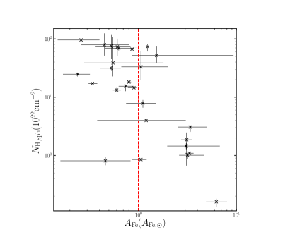
The overwhelming result is that a uniform spherical distribution of matter with solar abundances is ruled out in 8 out of 14 sources (corresponding to a total of 16 observations). The remaining 6 sources have at least one observation for which the Fe abundance is within 20% of the solar value, within the statistical errors. The sources with one such observation are 4U1908075, Cir X1, Cyg X1, Vela X1, while GX 3012 and Her X1 have two such observations each. This leaves 31 observations of these 6 sources for which the spherical, solar abundance model is rejected. Thus, we can say that 47 out of 56 spectra are not consistent with the Fe K emission line originating in a uniform spherical distribution of matter with an Fe abundance that is solar within 20%. These observations fit into two categories: either the derived Fe abundance is non-solar (by more than 20%), with robust lower and upper bounds, or the Fe abundance is unconstrained. The latter category is itself comprised of two sub-categories: one in which the Fe abundance only has a lower or upper bound, and one in which the Fe abundance has reached the maximum model table value of 10.0 . In the latter sub-category, the fitted column density is so small that the Fe abundance is driven to the highest value in the model table in order to attempt to account for the Fe K line flux, but this abundance is still insufficient to fit the line. In such cases (20 observations of 9 sources) we do not derive statistical errors for the other model parameters because the fit has failed in its objective to account for the Fe K line. There are 6 observations with only a lower or upper bound on the Fe abundance, leaving 20 observations of 11 sources that have a non-solar Fe abundance with both lower and upper bounds. These Fe abundance values range from a factor of to solar, i.e. from sub-solar to super-solar. The corresponding column density measurements, , range from cm-2 to cm-2, and Figure 1 shows plotted against the Fe abundance () measurements for all the observations that have both lower and upper bounds on both of the parameters. These Fe abundance measurements, especially the non-solar values, may of course be an artifact of fitting a model that is not appropriate. If we further stipulate that an apparently variable Fe abundance among different observations of the same source is not physical, we are left with only 3 sources out of the sample of 14 (4U170037, 4U1822371, GX 3012) that are consistent with a uniform, spherical distribution of matter, and of these only GX 3012 has an Fe abundance within 20% of the solar value. In fact, GX 3012 stands out as the only source that has an approximately solar Fe abundance in more than one observation. The derived Fe abundance for the one observation of 4U170037 is , and the Fe abundances for the three observations of 4U1822371 are all consistent with (see Table 5). These non-solar values may be artificial but it is not possible to determine this definitively with the current data. However, in Section 5.2 we will show the results of fitting these and other observations with a solar-abundance Compton reflector (using the mytorus model), as opposed to a reprocessor with a closed spherical geometry.
Table 5 (column 6) shows that the primary power-law continuum is generally very flat, and in about half of the spectra (27/56) reached 1.0, the lowest value in the bn11 table model. While this was adequate to describe the continuum, without higher energy spectral coverage it was not possible to better constrain the continuum. Hard power-law continua are not uncommon in X-ray binaries, and in particular for many of the sources in this paper (e.g. Oosterbroek et al., 2001; Chakrabarty et al., 2002; Boroson et al., 2003; Watanabe et al., 2003; Ji et al., 2011; Burderi et al., 2000; Neilsen et al., 2009; Smith et al., 2012; Grinberg et al., 2013; Paul et al., 2005).
Table 5 also indicates that about half of the observations (29/56) also require a second power law. As already mentioned, this is often required to fit a continuum rise in the soft part of the spectrum. However, 3 of these observations have , so that component might also be compensating for the inability of the bn11 model component photon index to access values harder than 1.0.
5.2 Overview of MYTORUS Model Results
Whereas many of the spectra that were fitted with the spherical bn11 model did not have sufficient column density to account for the Fe K line flux even for an Fe abundance as high as 10 , the mytorus model can provide unobscured lines of sight to a Compton reflection continuum and fluorescent line emission. The model is set up as described in Section 4.2 but it is important to note that since there are more free parameters than in the bn11 model, spectra in which the Fe K is not detected cannot provide useful constraints. In the bn11 model, due to the smaller number of parameters, the absence of an Fe K line provided constraints on the column density and Fe abundance. Therefore, the mytorus model is only applied to those observations listed in Table 1 that have a significant Fe K line detection, as defined in Section 4.3 (). We attempted to constrain the column density of the material out of the line of sight () but found that for most observations it could not be constrained and often had a spread of over two orders of magnitude. This is likely due to geometric degeneracies and the very limited HETG bandpass (see discussion at the beginning of Section 4). For these cases we fixed at 1025 cm-2 (the maximum allowed by the mytorus model), specifically testing the data against a Compton-thick reflection model. The exceptions were 4U170037, one observation of GX 3012, and one observation of Vela X1. The best-fitting results for all of the mytorus spectral fits are shown in Table 5.2. Our procedure for investigating involved obtaining a first, approximate, best-fit, before inspecting two-parameter, versus , confidence contours for each observation. If the 99% confidence contours were closed, then the best-fitting value of was used as a better initial guess for finalizing the fit, otherwise was fixed at 1025 cm-2.
C2cm cccc cccc cccc c
\tablecaptionFitting results for the uncoupled mytorus model (Murphy & Yaqoob, 2009)
\tablewidth0pc
\tabletypesize
\tablehead
\colheadSource
obs.
\colhead-stat(d.o.f)
\colheadgoodness
\colhead
\colhead
\colhead
\colhead
\colhead
\colhead
\colhead
\colhead
\colhead
\colhead \colhead
\colhead%
\colhead
\colhead
\colhead
\colhead(log)
\colhead
\colhead( cm-2)
\colhead( cm-2)
\colhead(1)
(2)
\colhead(3)
\colhead(4)
\colhead(5)
\colhead(6)
\colhead(7)
\colhead(8)
\colhead(9)
\colhead(10)
\colhead(11)
\startdata4U170037 657 A 1463.57(1437) 46.4
4U1822371 671 A 1501.90(1438) 78.5
4U1822371 9076 B 1495.11(1436) 79.8
4U1822371 9858 C 1567.21(1436) 98.3
4U1908075 5476 A 1517.84(1438) 40.4
4U1908075 5477 B 1289.84(1438) 94.7
4U1908075 6336 C 1571.48(1438) 80.0
Cen X3 1943 A 1780.34(1434) 100.0
Cen X3 705 B 1565.02(1430) 84.4
Cen X3 7511 C 1610.44(1428) 99.7
Cyg X1 11044 A 1692.59(1440) 100.0
Cyg X1 1511 F 1576.05(1438) 98.8
Cyg X1 2415 G 2051.46(1440) 100.0
Cyg X1 3407 K 1590.75(1436) 99.9
Cyg X1 3814 M 1471.92(1378) 93.3
Cyg X1 8525 N 1518.46(1348) 99.8
Cyg X1 9847 O 1549.62(1366) 99.8
Cyg X1 3815 P 1921.64(1314) 100.0
Cyg X3 101 A 1692.00(1433) 99.9
Cas 1895 A 1442.21(1374) 61.0
GX 3012 2733 B 2373.86(1405) 100.0
GX 3012 3433 C 1448.51(1422) 22.3
GX 14 2710 A 1524.86(1436) 87.5
GX 14 2744 B 1428.65(1438) 26.9
Her X1 2703 A 1684.08(1439) 98.9
Her X1 2704 B 1516.57(1439) 91.1
Her X1 2705 C 1640.76(1439) 85.0
Her X1 2749 D 1534.06(1438) 43.2
Her X1 3821 E 1570.57(1439) 94.8
Her X1 3822 F 1533.52(1436) 33.5
Her X1 4375 G 1494.95(1439) 75.0
Her X1 4585 H 1472.87(1436) 35.2
Her X1 6149 I 1670.44(1439) 99.8
Her X1 6150 J 1553.33(1436) 41.5
LMC X4 9571 A 1588.69(1437) 91.3
LMC X4 9573 B 1066.10(1438) 22.4
LMC X4 9574 C 1295.39(1437) 34.4
OAO 1657415 12460 A 1341.48(1438) 10.4
OAO 1657415 1947 B 1004.77(1438) 85.4
Vela X1 102 A 1360.28(1436) 88.0
Vela X1 14654 B 1715.27(1439) 100.0
Vela X1 1926 C 1842.27(1439) 100.0
Vela X1 1927 D 1718.44(1438) 100.0
Vela X1 1928 E 1454.03(1439) 53.9
\enddata\tabletypesize
\tablecommentsColumns (1) and (2) give the XRB system name, Chandra-HETG
observation ID, and associated alphabetical label used in this paper.
Columns (3) and (4) give the best-fit value of the -statistic, with
associated degrees of freedom, and the output of the xspec goodness command for 2000 random realizations of the data. Column
(5) gives the photon index for the direct, line-of-sight, zeroth-order
continuum. Column (6) gives the photon index for the
Compton-scattered, or “reflected” continuum. Column (7) gives the
photon index for any additional, “soft” power law continuum, and
column (8) the ratio of the normalizations of this continuum to that
of the direct continuum. Column (9) gives the relative normalization
factor for the Compton-scattered continuum. Columns (10) and (11) give
the equivalent neutral hydrogen column densities of the direct and
scattered components, respectively. The line shift and line width
parameters for each fit are shown in
Table 5.4.1. f: Parameter frozen; t: tied to
; d.o.f.: degrees of freedom. As explained in the text,
the mytorus model has only been applied to those observations
in Table 1 that have a significant Fe K line
detection (, Section 4.3).
For the same reason that was difficult to constrain, so was the continuum photon index , which had to be frozen at a value at one of the extreme ends of the allowed range (1.4 in 36 cases, and 2.6 in 6 cases). The line-of-sight column densities () were easier to constrain, and Table 5.2 shows that a wide range is found, from 0 to cm-2. Acceptable fits are obtained for all the observations, showing that an open, reflection-dominated geometry is generally viable, and in particular it is needed for the many cases for which a closed geometery, spherical model fails to explain the data. However, we stress that we are not inferring a literal physical interpretation of the data in terms of the mytorus model toroidal reflector, especially since the systematics resulting from limitations on the photon index are absorbed into the parameter . Rather, the success of the reflection-dominated fits should be seen as paving the way for more realistic and physically-motivated reflection models to be investigated in future work.
5.3 Comparison of the Spherical and MYTORUS Fits
From the results in Table 5 and Table 5.2, we see that for a given observation, the mytorus fit is statistically similar, or better than the corresponding bn11 fit, except for 5 observations of Her X1 (obs IDs 2703, 2705, 3821, 4375, and 6149) and 1 observation of GX 3012 (obs ID 2733). The residuals in the mytorus fits to the 5 observations of Her X1 correspond to excesses of data at the highest energies, relative to the model. This indicates that it is the restriction on the minimum value of the photon index for the Compton-scattered continuum () that is likely the cause of the mytorus fits being somewhat worse than the bn11 fits. In the case of GX 3012 (obs. ID. 2733), the mytorus is significantly worse than the bn11 fit, and it can be seen from the spectral plots in Appendix B that this is because the mytorus predicted model Fe K line flux falls substantially short of the data. There are some observations in which the mytorus fit is only marginally worse than the bn11 fit, but given the limitations placed on some of the parameters of the mytorus model, we do not interpret these differences as meaningful. We still conclude that the bn11 model is ruled out in the sources in which the Fe abundance is required to vary among observations of the same source. That leaves 4U1908075 (1 observation) and 4U1822371 (3 observations) that are consistent with bn11 models with non-solar Fe abundance, and GX 3012 (2 observations) with an Fe abundance within 20% of the solar value. The bn11 and mytorus fits are statistically similar for 4U1908075, 4U1822371, and GX 3012 (obs. ID. 3433). For GX 3012 (obs. ID. 2733), as mentioned above, the bn11 fit is significantly better than the mytorus fit. However, for GX 3012 (obs. ID. 3433), the mytorus fit is better than the bn11 fit, with being lower by 121.95 for the mytorus fit than for the bn11 fit, despite the fact that the bn11 model fit has only 2 more free parameters than the mytorus fit. The goodness values of the bn11 and mytorus fits are 99.6% and 28.3% respectively, further indicating that the mytorus fit is better than the bn11 fit. Also, from the spectral plots in Appendix B it can be seen that the poorer fit with the spherical model is due largely to a significant, broad excess in the –8 keV band compared to the mytorus fit.
5.4 The Fe K Line
The Fe K line is not detected in 12 observations according to the criterion (see Table 1). Specifically, the line is not detected in any of the 5 observations of Cir X1, and it is not detected in 7 out of 15 of the Cyg X1observations.
From the spectral fits described in Section 5.1 (bn11 model) and Section 5.2 (mytorus model), the detailed results for the parameters of the Fe K line are shown together for both models in Table 5.4.1. Shown are only results for observations in which the Fe K line was detected (based on the criterion), and in which, for the bn11 fit, the Fe abundance did not reach its maximum table value of 10 (since the latter condition indicates that the model failed to fit the Fe K line). Since a single number for the quality of each fit (“goodness” parameter in Table 5 and Table 5.2) does not necessarily indicate how well the model profile of the Fe K line fits the data, columns 11 and 12 in Table 5.4.1 show the maximum residual as a percentage of the model value in the energy range keV for the bn11 and mytorus models, respectively. In addition, for each observation and for both of the models, the data overlaid with the fitted models are shown in Appendix B zoomed in on the energy band containing the Fe K line. The quality of the fits to the detailed Fe K line profile are very important because one of the premises of our study is to determine what the fitted Fe K line model implies for the column density of the global matter distribution in each observation, and whether the resulting predicted model continuum does not conflict with the observed spectrum.
5.4.1 Fe K Line Shift and Peak Energy
For both the bn11 and mytorus models, the fitted shifts of the
Fe K line peak energy, , are shown in Table 5.4.1, in
columns 3 and 4, respectively. The equivalent velocity shifts are
shown in columns 5 and 6 of Table 5.4.1 for the bn11 and
mytorus models, respectively. In
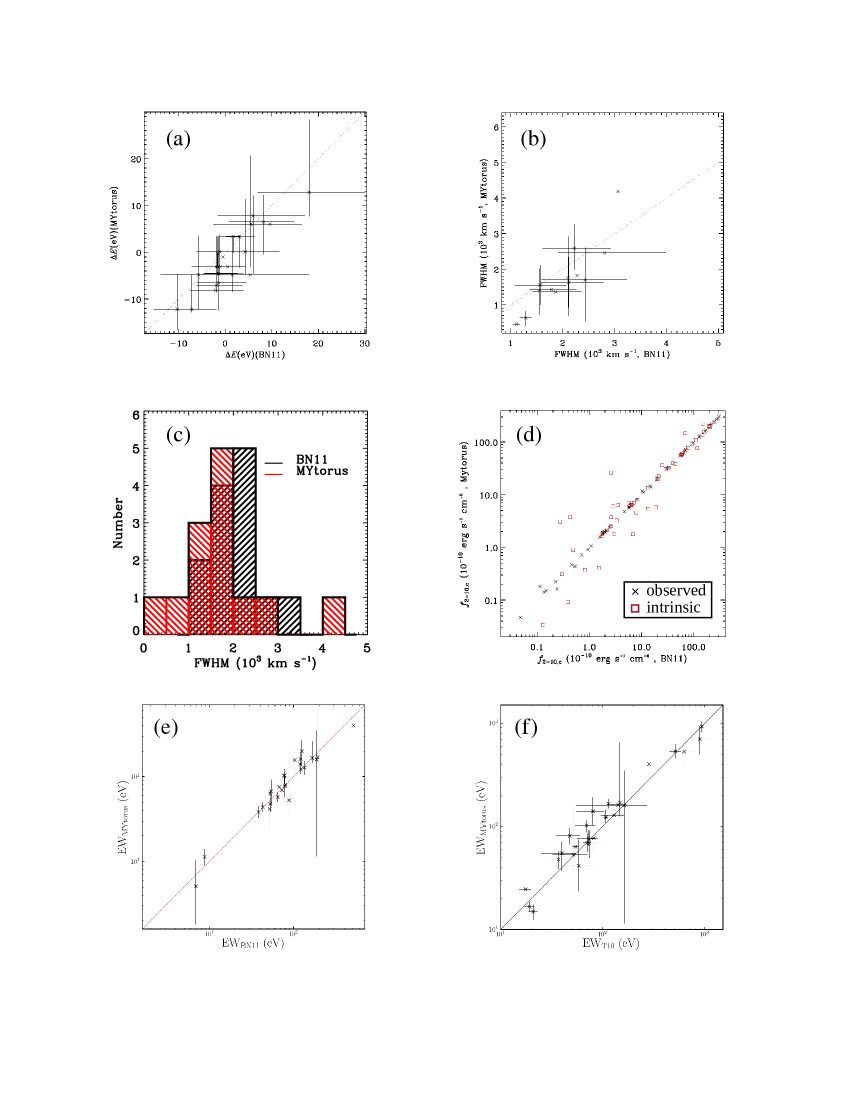
Figure 2, panel (a),
the energy shifts from the
mytorus model are plotted against the corresponding shifts obtained from
the bn11 model. It can be seen that the shifts from the bn11 model
are systematically higher than those from the mytorus model by eV.
However, as explained in Section 4.1, this is expected
because of the less accurate and less detailed representation of the Fe K line
in the bn11 model table. Despite the offset, the relation between the
shifts from one model versus the other follows a linear trend. The
shifts are spread in the approximate range of eV, with one
outlier at eV (bn11 model). This supports the
origin of the Fe K line in essentially neutral matter. The shifts
are not biased in the positive or negative directions. They could be
due to systematic errors in the energy scale, mild ionization, or
small velocity shifts. Mild ionization actually results in a negative
shift of up to eV for ionization states up to Fe ix,
{longrotatetable}
{deluxetable*}C1.4cm cccc cccc cc@ c @c@c@c@c@ c@
\tablecaptionProperties of Narrow Fe K line
\tabletypesize
\tablehead
\colheadSource
obs.
FWHM
residuals
Flux
EW
\colhead
\colhead
\colhead (eV)
(km s-1)
(eV)
(km s-1)
(%)
(photons cm-2 s-1)
(eV)
\colhead
\colhead
\colhead \colheadbn11\colheadmyt
\colheadbn11\colheadmyt
\colheadbn11\colheadmyt
\colheadbn11\colheadmyt
\colheadbn11\colheadmyt
\colheadbn11\colheadmyt
\colheadbn11\colheadmyt
\colhead(1)
(2)
\colhead(3)
\colhead(4)
\colhead(5)
\colhead(6)
\colhead(7)
\colhead(8)
\colhead(9)
\colhead(10)
\colhead(11)
\colhead(12)
\colhead(13)
\colhead(14)
\colhead(15)
\colhead(16)
\decimals\startdata4U170037 657 A 4.1 4.0 9.49 72.7
4U1822371 671 A 2.4 2.3 4.42 52.7
4U1822371 9076 B 1.4 1.4 2.85 38.1
4U1822371 9858 C 1.5 1.6 3.30 43.0
4U1908075 5476 A 3.0 3.2 4.32 119.4
4U1908075 5477 B 1.1 1.0 0.63 51.9
4U1908075 6336 C 0.9 0.9 1.33 78.7
Cen X3 1943 A 18.4 9.2 6.41 7.8
Cen X3 705 B 1.5 1.7 3.02 79.4
Cen X3 7511 C 9.0 4.4 11.18 59.3
Cyg X1 11044 A 13.9 13.4 1.72 2.6
Cyg X1 1511 F 13.2 13.2 4.20 6.8
Cyg X1 2415 G 10.4 11.6 0.86 0.9
Cyg X1 3407 K 12.5 10.2 9.27 6.9
Cyg X1 3814 M 6.4 6.3 9.45 14.6
Cyg X1 8525 N 12.9 12.0 5.88 8.8
Cyg X1 9847 O 16.9 12.1 15.91 19.5
Cyg X1 3815 P 7.1 6.7 15.01 14.4
Cyg X3 101 A 24.5 26.1 37.98 81.2
Cas 1895 A 1.4 1.0 0.34 19.5
GX 3012 2733 B 12.6 30.3 103.50 515.0
GX 3012 3433 C 6.4 5.4 40.89 166.4
GX 14 2710 A 1.0 0.8 1.65 67.1
GX 14 2744 B 7.2 4.4 15.40 162.7
Her X1 2703 A 4.2 4.6 3.23 102.7
Her X1 2704 B 9.3 8.0 4.00 16.3
Her X1 2705 C 1.2 1.3 0.80 125.0
Her X1 2749 D 1.3 1.1 3.21 456.1
Her X1 3821 E 2.0 1.9 3.63 120.5
Her X1 3822 F 2.6 2.0 6.16 187.8
Her X1 4375 G 3.8 4.3 6.36 77.9
Her X1 4585 H 4.8 3.7 6.79 88.1
Her X1 6149 I 4.5 4.2 6.62 77.2
Her X1 6150 J 1.7 1.7 3.86 133.4
LMC X4 9571 A 0.9 0.9 0.68 54.2
LMC X4 9573 B 0.4 0.4 0.43 516.7
LMC X4 9574 C 0.6 0.6 0.36 149.6
OAO 1657415 12460 A 2.7 3.9 6.45 1427.9
OAO 1657415 1947 B 3.5 3.8 7.02 191.6
Vela X1 102 A 1.0 1.0 1.39 677.7
Vela X1 14654 B 3.5 4.1 11.69 64.8
Vela X1 1926 C 0.4 0.6 1.83 740.8
Vela X1 1927 D 10.0 11.6 38.95 121.6
Vela X1 1928 E 5.9 7.7 20.73 52.6
\enddata\tabletypesize
\tablecommentsThe table only includes significant detections. Columns (1) and (2)
give the XRB system name, Chandra-HETG observation ID, and associated
alphabetical label used in this paper. Except for columns (1) and
(2), columns show pairs of results for the same parameter in the
spherical (bn11) and mytorus (myt) model. Thus, columns (3) and (4)
give the line’s peak energy shift, and columns (5) and (6) the line’s
velocity shift, all calculated from the models’ best-fit redshift
parameters. Columns (7) and (8) give the energy width of the line’s
Gaussian convolution kernel (Section 4.5). Columns (9) and
(10) give the line’s velocity with, calculated from the values in
columns (7) and (8). Columns (11) and (12) give the maximum residuals
as a percentage of the model value in the vicinity of the Fe K line
(energy range keV). Columns (13) and (14) give the flux of
the Fe K line. Columns (15) and (16) give the Fe K line equivalent
width.
5.4.2 Fe K Line Flux and Equivalent Width
The flux of the Fe K line for each observation and for each of the two models (bn11 and mytorus) is given in columns 13 and 14 of Table 5.4.1. Also given in Table 5.4.1 are the EW values of the Fe K line for each observation and each model (columns 15 and 16). The fluxes and EWs were derived using the methods decribed in Section 4.6, and Table 5.4.1 includes those observations for which the Fe abundance in the bn11 spherical model fits reached the maximum value of 10 . The bn11 model parameters for these observations are given for reference only and are not meaningful because the model did not fit the Fe K line (they can be identified in Table 5.4.1 by the fact that their bn11 parameters have no statistical errors). The Fe K line fluxes and EW values from the mytorus model are therefore the most reliable for examining consistently derived values for the largest number of sources in the sample. These Fe K line fluxes span a range of a factor of from to photons cm-2 s-1, and the EW values span a range of a factor of , from eV to keV. In Figure 2, panel (e), we show the EW measurements from the mytorus model versus those from the bn11 model, for those observations that had valid measurements of EW from the bn11 model. The agreement with the line of equality in the diagram demonstrates the consistency of the EW values inferred from the two models for this subset of the observations. In general, large values of the EW of the order of 1 keV or higher are associated with reflection-dominated X-ray spectra regardless of geometry, and smaller values of EW of the order of 10s of eV are associated with spectra that are dominated by a direct continuum that swamps the reflection continuum.
In Figure 2, panel (f), we show the EW measurements from the mytorus model versus those from the Gaussian modeling of T10 (their Table 2) for the 26 observations that have valid results in both papers. There appears to be consistency of the EW values inferred from these two models for this subset of the observations as well, although for ten observations at EW values eV the T10 values are too low with respect to the line of equality even when quoted errors are taken into account. However, we do not expect agreement between the T10 and mytorus EW values in every case because (a) in many cases T10 fix the line width to unresolved ( Å), and (b) they do not include a Compton shoulder.
An inspection of column (16) in Table 5.4.1 reveals that five observations show extreme values of eV444A sixth observation with an extreme value, LMC X4 (obs. ID. 9574), has an upper 90% EW uncertainty that is too large, and is not shown in panels (e) and (f) of Figure 2.. These extreme EW values are consistent with variability in the line-of-sight extinction of the direct continuum for all of these sources, associated with absorption clumps in the line of sight, located in the stellar wind from the non-compact companion, on the companion surface, and/or an accretion disk. Although these large values appear across fitted models, including the bn11 model and the Gaussian Fe K modeling of T10, it is worth noting that the decoupled mytorus setup used here, specifically mimics a clumpy reprocessor distribution. These observations and the interpretation of the EW values are discussed in greater detail in Section A.9 for GX 3012 (obs. ID. 2733), Section A.11.4 for Her X1 (obs. ID. 2749), Section A.12 for LMC X4 (obs. ID. 9573), Section A.13 for OAO 1657415 (obs. ID. 12460), Section A.14.1 for Vela X1 (obs. ID. 102) and Section A.14.3 for Vela X1 (obs. ID. 1926).
5.4.3 Fe K Line Width
The Fe K line width parameter (see Section 4.5) is shown in columns 7 and 8 of Table 5.4.1 for the bn11 and mytorus models, respectively. The corresponding pairs of FWHM are shown in columns 9 and 10. In Figure 2, panel (b), we show the FWHM obtained from the mytorus model plotted against the FWHM obtained from bn11 model, for those observations for which both a lower and upper bound could be obtained for both models. In the remaining cases there is either only an upper limit on the FWHM or else it could not be constrained and was fixed at . It can be seen from Figure 2, panel (b), that the FWHM values obtained from the mytorus model are systematically smaller than the corresponding values obtained from the bn11 model. This is expected because, as explained in Section 4, the implementation of the Fe K in the mytorus model tables is more accurate than that in the bn11 model table. The latter represents the Fe K line as a single component, whereas the mytorus model represents the line as the K and K doublet, each component of the doublet having its own Compton shoulder. Also, the energy grid points representing the Fe K line in the bn11 model are much coarser than those in the mytorus model. Therefore, hereafter, we take the FWHM values from the mytorus model as providing the best indicators of the velocity dispersion of the matter distribution responsible for producing the Fe K line. The approximate range in FWHM among the observations represented in Figure 2, panel (b), is . The distributions of FWHM measurements in histogram form are shown in Figure 2, panel (c). The histograms do not include observations for which the FWHM has lower and/or upper bounds for only one of the models.
C1.4cm c cc cc cc cc c
\tablecaptionContinuum fluxes
\tabletypesize
\tablehead
\colheadSource
obs.
\colhead
\colhead
\colhead (log erg cm-2 s-1)
(log erg cm-2 s-1)
(log erg s-1)
(log erg s-1)
\colhead
\colhead
\colhead \colheadbn11\colheadmyt
\colheadbn11\colheadmyt
\colheadbn11\colheadmyt
\colheadbn11\colheadmyt
\colhead(1)
(2)
\colhead(3)
\colhead(4)
\colhead(5)
\colhead(6)
\colhead(7)
\colhead(8)
\colhead(9)
\colhead(10)
\startdata4U170037 657 A
4U1822371 671 A
4U1822371 9076 B
4U1822371 9858 C
4U1908075 5476 A
4U1908075 5477 B
4U1908075 6336 C
Cen X3 1943 A
Cen X3 705 B
Cen X3 7511 C
Cir X1 12235 A
Cir X1 1905 B
Cir X1 1906 C
Cir X1 1907 D
Cir X1 8993 G
Cyg X1 11044 A
Cyg X1 12313 B
Cyg X1 12314 C
Cyg X1 12472 D
Cyg X1 13219 E
Cyg X1 1511 F
Cyg X1 2415 G
Cyg X1 2741 H
Cyg X1 2742 I
Cyg X1 2743 J
Cyg X1 3407 K
Cyg X1 3814 M
Cyg X1 8525 N
Cyg X1 9847 O
Cyg X1 3815 P
Cyg X3 101 A
Cas 1895 A
GX 3012 2733 B
GX 3012 3433 C
GX 14 2710 A
GX 14 2744 B
Her X1 2703 A
Her X1 2704 B
Her X1 2705 C
Her X1 2749 D
Her X1 3821 E
Her X1 3822 F
Her X1 4375 G
Her X1 4585 H
Her X1 6149 I
Her X1 6150 J
LMC X4 9571 A
LMC X4 9573 B
LMC X4 9574 C
OAO 1657415 12460 A
OAO 1657415 1947 B
Vela X1 102 A
Vela X1 14654 B
Vela X1 1926 C
Vela X1 1927 D
Vela X1 1928 E
\enddata\tabletypesize
\tablecommentsColumns (1) and (2) give the XRB system name, Chandra-HETG
observation ID, and associated alphabetical label used in this
paper. Except for columns (1) and (2), columns show pairs of results
for the same parameter in the spherical (bn11) and mytorus (myt)
model. The energy band for all quantities is keV
(Section 4.7). Thus, columns (3) and (4) give the total
observed continuum flux, and columns (5) and (6) the total intrinsic
continuum flux. Columns (7) and (8) give the observed luminosities
corresponding to the fluxes in columns (3) and (4), and columns (9) and
(10) the intrinsic luminosities corresponding to the fluxes in columns
(5) and (6).
In order to determine more rigorously whether the Fe K line is resolved in a given observation, we must take into consideration the fact that the Compton shoulder of the Fe K line has a direct impact on the inferred velocity width. Since the strentgh of the Compton shoulder relative to the line core depends on the column density of the material in which the line is formed, we examine confidence contours of FWHM (from the mytorus model) versus the mytorus column density, . The mytorus model self-consistently calculates the Compton shoulder for each component of the Fe K doublet so there is no arbitrary ad hoc parameter controlling the magnitude of the shoulders relative to the line cores. The two-parameter confidence contours of FWHM versus (for 68%, 90%, and 99% confidence) are shown in Appendix C for every observation in which the Fe K line was detected. At 99% confidence, we can infer the following. The contours show that the Fe K line is unresolved in all of the observations of 5 sources, namely 4U170037, Cas, GX 1+4, OAO 1657415, and Vela X1. They also show that the Fe K line is resolved in all observations of 2 sources, namely Cyg X3 and GX 3012. In 5 sources the Fe K line is resolved in some of the observations and unresolved in the remaining observations of a given source. These 5 sources are 4U1822371, 4U1908075, Cen X3, Her X1 and LMCX4, and the upper limits on the FWHM for the unresolved line cases are in the range . The contours for Cyg X1 show that the Fe K line is resolved in 2 observations of the source, but the FWHM had to be fixed at 100 km s-1 in 4 of the remaining 6 observations because it could not be constrained. In Cir X1, the Fe K line was not detected in any of the observations.
5.5 Continuum
As described in Sections 4.2 and 5.1, many of the X-ray spectra in the sample are very hard with a photon index , and in some cases the photon index reaches the lower limit of of the bn11 table model. Although such flat spectra are not unusual for the sources in the sample, the fitted models may only be empirical descriptions, and the photon indices are often very poorly constrained due to the lack of data beyond the Chandra HETG bandpass.
Thus, continuum fluxes and luminosities based on the extrapolation of the model spectra beyond keV would not be reliable. We give the 2–10 keV observed and intrinsic continuum fluxes and luminosities for both the bn11 and mytorus models in Table 5.4.3 (see Section 4.7 for details of how they are derived). In Figure 2, panel (d), we show the observed and intrinsic continuum fluxes from the mytorus model against the corresponding quantities obtained from the bn11 model fits. The fluxes span a range of orders of magnitude, from to . As expected there is good agreement between the observed fluxes from the bn11 and mytorus models because all models that give good fits to the data should empirically return consistent fluxes since the models have to follow the same data. However, intrinsic fluxes (i.e. corrected for absorption and reflection) are highly model-dependent. In the case of the bn11 and mytorus models, the intrinsic luminosties are most divergent when the two models involve very different magnitudes of absorption and/or reflection.
5.6 Line-Emitting Region Size Constraints
Although the kinematics of the matter distribution producing the Fe K line is unknown, we can perform a simple exercise to estimate the size of the matter distribution under the assumption of Keplerian motion. Specifically, we can use Fe K line FWHM measurements derived in Section 5.4.3, combined with mass estimates of the central compact object, assuming that the line-emitting material is virialized (e.g., as in Shu et al., 2011). If the velocity dispersion is , the distance, of this material to a compact object of mass can be estimated via the relation . Further assuming that the velocity dispersion is related to FWHM velocity by (as in Netzer et al., 1990), we obtain , where the gravitational radius . The results of the calculations are shown in Table 5.6, in which columns 3 and 4 show the radius in gravitational radii units for the bn11 and mytorus models respectively. The radius of the line-emitting region in units of gravitational radii does not of course depend on the mass of the compact object. The calculated radii range from thousands to tens of thousands gravitational radii. In order to estimate the radii in absolute units, we searched the literature and compiled mass estimates of the compact object for each source in our sample. The masses and references to the literature are shown in Table 5.6. Since, in many cases, a range in mass estimates exists for a give source, resulting from different studies, we performed calculations for the lowest available mass estimate (, giving a radius ), and for the highest available mass estimate (, giving a radius ). Values of for the two models are shown in columns 6 and 7 of Table 5.6, and values of are shown in columns 9 and 10 of Table 5.6. The values of and are typically of the order of km.
C1.2cm C1cm cc c cccccc
\tablecaptionFWHM and deduced radius of line emitting region for the
Fe K line
\tabletypesize
\tablehead
\colheadSource
obs.
\colhead
\colhead
\colhead
\colhead
\colhead ()
\colhead()
( km)
\colhead()
( km)
\colhead
\colhead
\colhead \colheadbn11\colheadmyt
\colhead
\colheadbn11\colheadmyt
\colhead
\colheadbn11\colheadmyt
\colhead(1)
(2)
\colhead(3)
\colhead(4)
\colhead(5)
\colhead(6)
\colhead(7)
\colhead(8)
\colhead(9)
\colhead(10)
\startdata4U170037 657 A
4U1822371 671 A
4U1822371 9076 B
4U1822371 9858 C
4U1908075 5476 A
4U1908075 5477 B
4U1908075 6336 C
Cen X3 1943 A
Cen X3 705 B
Cen X3 7511 C
Cyg X1 3814 M
Cyg X1 9847 O
Cyg X1 3815 P
Cyg X3 101 A
Cas 1895 A
GX 3012 2733 B
GX 3012 3433 C
GX 14 2710 A
GX 14 2744 B
Her X1 2705 C
Her X1 2749 D
Her X1 3821 E
Her X1 3822 F
Her X1 4375 G
Her X1 4585 H
Her X1 6149 I
Her X1 6150 J
LMC X4 9571 A
LMC X4 9573 B
OAO 1657415 12460 A
OAO 1657415 1947 B
Vela X1 102 A
Vela X1 14654 B
Vela X1 1927 D
Vela X1 1928 E
\enddata\tablecomments
Cases for which the FWHM was frozen in the fit are not
included, unless FWHM errors were obtained for one of the
models.
Columns (1) and (2) give the XRB system name, Chandra-HETG
observation ID, and associated alphabetical label used in this
paper. Columns (3), (4), (6), (7), (9) and (10) show pairs of results
for the same parameter in the spherical (bn11) and mytorus (myt)
model.
Columns (3) and (4) give the radius in units of , where
the gravitational radius .
Column (5) gives the lowest compact object mass estimate, ,
available in the literature. Columns (6) and (7) give the radius in
km, assuming the value from column (5). Column (8) gives the
highest compact object mass estimate, , if available in the
literature. Columns (9) and (10) give the radius in km, assuming
the value from column (8), where available.
Letter notes are as in
Table 5, except for c, indicating that a “canonical”
compact object mass was assumed. and references- 1:
Falanga et al. (2015), 2: Clark et al. (2002), 3:
Jonker et al. (2003), 4: Muñoz-Darias et al. (2005), 5:
Ash et al. (1999), 6:
Herrero et al. (1995), 7: Orosz et al. (2011), 8:
Vilhu et al. (2009); 9: Smith et al. (2012); 10:
Harmanec et al. (2000); 11: Kaper et al. (2006); 12:
Hinkle et al. (2006); 13: Leahy & Abdallah (2014); 14:
van der Meer et al. (2007); 15: Mason et al. (2012); 16:
Rawls et al. (2011).
6 Summary and Conclusions
In the present work, we tested two specific conclusions of a study by Torrejón et al. (2010) of the Chandra High Energy Grating (HEG) spectra of 14 X-ray binaries that exhibit Fe K line emission from matter surrounding the accretion flow onto the compact object in each source. The first is their conclusion that all observations of the 14 sources were consistent with the Fe K line originating in a uniform spherical distribution of matter with solar Fe abundance. However, this conclusion was based on ad hoc models that did not self-consistently treat the Fe K line emission, absoprtion, and Compton scattering. Their second conclusion was that all of the Fe K emission lines were unresolved by the HEG (which has a spectral resolution FWHM at 6.4 keV). In our study we used 56 HEG observations of the same 14 sources on which the conclusions of Torrejón et al. (2010) were based. However, instead of using unphysical, ad hoc models we applied the Brightman & Nandra (2011) self-consistent model of a spherical, uniform distribution of matter to the spectra. We also tested the data against a solar-abundance Compton-thick toroidal reflector model (implemented with the mytorus model of Murphy & Yaqoob, 2009). In addition, we rigorously investigated the confidence contours of the FWHM of the Fe K line versus the global column density for both models. Our results can be summarized as follows.
-
1.
The Fe K line was not detected in all 5 observations of Cir X1, and 7 out of 15 observations of Cyg X1.
-
2.
Only 1 source out of the 14, GX 3012, is consistent with a uniform spherical distribution of matter with the abundance of Fe within 20% of the solar value. However, 1 of the 2 observations of GX 3012 is better described by a solar-abundance, Compton-thick reflection model.
-
3.
Two sources, 4U170037 and 4U1822371, are consistent with a uniform spherical distribution with a non-solar Fe abundance. This abundance relative to solar is for 4U170037 and for all 3 observations of 4U1822371.
-
4.
A uniform, spherical distribution of matter is ruled out for the remaining 11 sources because a variable Fe abundance among different observations is required. Of these 11 sources, 5 have at least one observation that happens to have an abundance of Fe that is within 20% of the solar value.
-
5.
There are 20 observations of 9 sources for which the Fe abundance in the uniform spherical model reached 10 , the maximum value allowed by the model. These 9 sources are among the 11 that are already rejected on the basis that the Fe abundance is required to vary between observations.
-
6.
The Fe K line is unresolved in all of the observations of 5 sources, namely 4U170037, Cas, GX 1+4, OAO 1657415, and Vela X1.
-
7.
The Fe K line is resolved in all observations of 2 sources, namely Cyg X3 and GX 3012.
-
8.
In 5 sources the Fe K line is resolved in some of the observations and unresolved in the remaining observations of a given source. These 5 sources are 4U1822371, 4U1908075, Cen X3, Her X1, and LMCX4.
-
9.
In Cyg X1, among the observations in which the Fe K line was detected, it was resolved in 2 observations, but the line width could not be constrained and had to be fixed in 4 out of the 6 remaining observations.
-
10.
Among the observations in which the Fe K line was resolved, the FWHM covers a wide range, .
-
11.
If the matter distribution is virialized, the FWHM measurements imply a size range of thousands to tens of thousands gravitational radii. Using black-hole and neutron-star mass estimates in the literature, this typically corresponds to a range of to .
-
12.
The spherical X-ray reprocessor model of Brightman & Nandra (2011) introduces artificial energy shifts and broadening of the Fe K line when fitted to HETG data because of the over-simplified implementation of the Fe K line in this model. Specifically, the energy grid in the model table covering the Fe K line is too coarse, and the Fe K line is modeled as a single component instead of the doublet, with components K and K that are separated by eV. The mytorus model implements a much more accurate treatment of the Fe K line and so does not suffer from these systematic effects.
-
13.
Although the mytorus model provides a better or statistically similar fit for the majority of observations, there are limitations in the mytorus model and the energy bandpass of the HEG data that are important to address in future work. Our results should be interpreted as a motivation to apply more physically realistic models to spectra with a wider bandpass, while still retaining sufficient spectral resolution and throughput in the Fe K band.
Acknowledgements.
We would like to thank the anonymous referee for their constructive comments and support. We also thank Mihoko Yukita, Keith Arnaud and David Huenemoerder for useful discussions. Support for this work was provided by the National Aeronautics and Space Administration through Chandra Award Number AR4-15002A issued by the Chandra X-ray Observatory Center, which is operated by the Smithsonian Astrophysical Observatory for and on behalf of the National Aeronautics and Space Administration under contract NAS8-03060. The scientific results reported in this article are based on data obtained from the Chandra Data Archive. \facilitiesChandra.
Appendix A
Details on Individual Sources and Observations
This Appendix presents specific details on spectral fitting of individual observations for all targets in this paper, as well as some historical information and context for each source. Our results are based on fitting the uniform spherical model (see Section 4.1) and the mytorus toroidal X-ray reprocessor model (see Section 4.2). We do not directly compare the various column densities we obtain from our fits with previous work on the same data that applied ad hoc, phenomenological models because such a comparison is not meaningful. Only column densities obtained with the same model are comparable but none of the previous works on the sources in our sample apply the models that we do. We also note that the precision of Fe K line EW values in T10 is over-stated compared to the statistical errors, but we nevertheless quote exact values given by T10 whenever we compare our EW values with those of T10. We note that existing X-ray spectroscopy in the literature for some observations of some of the sources was performed on spectra selected by orbital phase rather than by observation IDs. Phase-resolved spectroscopy is beyond the scope of our present study, whose primary goal is to test the assertion by T10 that the circumstellar matter distribution in all of the X-ray binaries in our sample is consistent with a uniform, solar-abundance sphere. If the assertion is true, the orbital phase should be irrelevant. However, accounting for observation phase can help understand the extreme EW values ( eV) registered for six of these observations (Section 5.4.2). Thus, in the interest of completeness some phase-resolved spectroscopy results are taken into account in the discussion of these specific observations below.
In the mytorus spectral fits, unless otherwise stated, the toroidal column density, , is fixed at cm-2 because in most cases the limited bandpass of the data makes this parameter poorly constrained, leading to unstable fits.
In some of the spectra, in addition to the basic X-ray reprocessor model and its associated fluorescent emission lines, additional emission lines are detected due to ionized Fe. These are discussed on a case-by-case basis whenever the data required the additional model components. The parameters for these extra emission lines are not given for the sake of clarity of presentation of the complex results. Moreover, those paramaters do not affect our inferences of the properties of the matter distribution producing the Fe K emission line, which is the primary focus of our study.
Regarding our analysis results, when we refer to the Fe K line being resolved by the HEG we specifically mean that the two-parameter, 99% confidence contour of FWHM versus (the equatorial column density in the mytorus model) is greater than zero. We showed in Section 4 that the Fe K line width derived from the mytorus is more accurate than that derived from the bn11 model because the implementation of the Fe K line profile in the bn11 model is compromised by approximations discussed in Section 4. The spectral resolution of the HEG is km s-1 FWHM at 6.4 keV. Most of our Fe K line width measurements cannot be compared with previous work because the HEG line width for the sources in our sample has not been rigorously measured before for most of the sources in the sample.
In the last few years, a number of papers have presented analyses for some of these objects using broadband X-ray data from missions such as NuSTAR or Suzaku. Thus Jaisawal & Naik (2015) analyze Suzaku data for 4U170037; Sasano et al. (2014) analyze Suzaku data for 4U1822371; Naik et al. (2011) analyze Suzaku, and Farinelli et al. (2016) Suzaku and NuSTAR data for Cen X3; Tomsick et al. (2014) and Parker et al. (2015) analyze Suzaku and NuSTAR data for Cyg X1, while Walton et al. (2016) NuSTAR-only data for the same object; Suchy et al. (2012) analyze Suzaku data for GX 3012; Yoshida et al. (2017) analyze Suzaku data for GX 1+4; Fürst et al. (2013) and Wolff et al. (2016) analyze NuSTAR, and Farinelli et al. (2016) Suzaku and NuSTAR data for Her X1; Shtykovsky et al. (2017) analyze NuSTAR, and Hung et al. (2010) Suzaku data for LMCX4; Jaisawal & Naik (2014) and Pradhan et al. (2014) analyze Suzaku data for OAO 1657415; and Maitra & Paul (2013) analyze Suzaku data for Vela X1.
None of these works use either the bn11 or the mytorus model employed in the present paper. It is also important to stress that the photon indices in these papers are not directly comparable to ours, which reflect a limited energy range, and cannot be extrapolated to calculate fluxes and luminosities over more extended energy ranges.
A.1 4U170037
This is a supergiant, eclipsing XRB with a single HETG observation in our sample, obs. ID. 657. There is debate in the literature for the type, as well as the mass, of the compact object. The most recent result is for a neutron star by Falanga et al. (2015), with , based on more than ten years of monitoring observations with RXTE and INTEGRAL to refine orbital parameter determination. We also use the earlier determination of Clark et al. (2002) of a higher mass ( ), suggesting that this compact object is in a grey area between high-mass neutron stars and low-mass black holes. This work is based on a detailed non-LTE analysis of the ultraviolet and optical spectrum of the O-type high-mass donor of this system.
Boroson et al. (2003) analyze the same HETG observation as in our sample, splitting it into three segments, namely “flaring” (F), “quiescent” (Q), and “ending” (E). They further subdivide F to a “high” (H) and “low” (L) state, and E to an EL state. The Fe K line centroid energy ranges from Å to Å (or keV), and the FWHM from to km s-1 for E and F, respectively. The line is unresolved in their EL state. The line flux ranges from to photons cm-2 s-1 for EL and FH, respectively (Boroson et al. 2003 did not give EW values).
For this observation T10 obtained a line centroid of Å ( keV), a line flux of photons cm-2 s-1, and an EW of eV.
In our analysis, the bn11 model fits the data well with an iron abundance of solar. Although the Fe K line is resolved in the bn11 fit, in the mytorus fit the Fe K line is unresolved, with an upper limit on the FWHM of . Overall, there are two distinct solutions for the mytorus fit, one with a low value of and one with a high value ( and cm-2 respectively). We choose the low- solution for which we give fit results, as this corresponds to a larger, more conservative and FWHM upper limit555Note that, unlike a few other cases with two possible solutions, the high- solution here does not reach the mytorus model’s upper bound, cm-2, which we normally chose in such cases.. The Fe K line fluxes from both bn11 and mytorus fits are consistent with those obtained by Boroson et al. (2003) and T10, both of which used ad hoc, phenomenological models, and our Fe K EWs are consistent with the value given by T10.
van der Meer et al. (2005) calculate intrinsic fluxes in the keV band with XMM-Newton, ranging from to erg cm-2 s-1, depending on model and observation phase. These overlap with our result of erg cm-2 s-1 obtained for our single observation with mytorus, although in the keV band.
A.2 4U1822371
This object belongs to the rare class of eclipsing LMXBs. It is also the prototypical Compton-thick accretion disk corona (ADC) source, for which only X-rays scattered from material above and below the accretion disk are thought to be able to reach the observer (White & Holt, 1982).
There is a range of mass estimates for the neutron star compact object in the literature. Jonker et al. (2003) combine radial velocity estimates from optical spectroscopic observations with pulse timing analysis to obtain a lower limit of . Muñoz-Darias et al. (2005) model the “K-correction” for emission lines to obtain a range . This range includes the most recent estimate of (Iaria et al., 2015) from X-ray-based estimates of the spin period and its derivative.
There are 3 HETG observations of 4U1822371 in our sample (see Table 1). For obs. ID. 671 the combined Medium- and High-Energy Transmission Grating analysis of Cottam et al. (2001) obtains an upper limit to the Fe K line broadening of 1500 km s-1. These authors also split the observation into different phases, always obtaining a line centroid consistent with 1.935 Å (6.407 keV). Ji et al. (2011) use all 3 observations and divide them into five phases and obtain Fe K line wavelengths ranging from –Å (or 6.378–6.404 keV). In one case the Fe K line is resolved, with Å, or666Ji et al. (2011) use an undefined symbol throughout, with values in Å. For conversion to velocities, we assume here that this represents FWHM. . In two cases the line is unresolved, with only an upper limit on the width, the largest being Å, corresponding to a FWHM of 1115 km s-1. In the other two cases the width is simply given as Å (or ), with no statistical errors.
T10 also only analyze obs. ID. 671, obtaining a centroid of Å ( keV) for the Fe K line, a flux of photons cm-2 s-1, and an EW of eV.
Finally, Iaria et al. (2013) use an average HETG spectrum from obs. ID. 9858 and obs. ID. 9076 and obtain a line energy of keV, line width eV or FWHM , EW eV, and an estimated Keplerian region radius of cm.
As discussed by Cottam et al. (2001), the HEG spectra for this object show discrete emission lines for a range of abundant elements. In particular, both Fe K and Fe xxvi emission lines are detected, which clearly originate in regions with completely different ionization states. The lines are reported to be persistent through all orbital phases, although their intensities vary (Ji et al., 2011). In our analysis, we utilize all 3 HETG observations (obs. IDs. 671, 9858, and 9076) and for both the bn11 and mytorus models, we include a Gaussian component to fit the high-ionization He-like line at an energy of keV. We find that the Fe K line is unresolved in obs. ID. 671 but resolved in the other two observations, with the FWHM being – (see Table 5.4.1 and Figure C.1 in Appendix C). The Fe K line fluxes and EW values we obtain for both models are consistent with values in the literature derived from fitting phenomenological models, as described above. Our bn11 fits yield an Fe abundance relative to solar of for each of the three HETG observations, so a uniform, solar-abundance spherical matter distribution is ruled out.
A.3 4U1908075
This XRB belongs to the rare class of HMXBs with an OB-supergiant companion (Levine et al., 2004; Morel & Grosdidier, 2005). There are no mass estimates for the primary of this source in the literature. Following standard practice, we assume a canonical neutron-star mass of 1.4 (e.g. Levine et al., 2004; Morel & Grosdidier, 2005; Martínez-Núñez et al., 2015). The X-ray emission is hard and highly absorbed with a column density varying by factors of a few between phases.
Among the 3 HETG observations of this source in the present study, the bn11 model requires an Fe abundance that varies among observations, from –3 solar, so we reject the uniform, spherical, model (see Table 5). In the mytorus fits the line-of-sight column density varies between observations (as found from previous studies) and the Fe K line flux varies by an order of magnitude (the latter is consistent with the phenomenological modeling of T10). The mytorus fits, corresponding to a Compton-thick reflector with an Fe abundance that is solar, work because the line-of-sight absorption is decoupled from the global column density. In contrast, in the spherical model, the line-of-sight absorption, which affects the low-energy continuum shape, is the same as the global column density, which affects the flux of the Fe K line. In order to remain self-consistent, the spherical model can only vary the Fe abundance in order to try to fit the Fe K line flux with a column density that must also explain the shape of the contnuum. We note that obs. IDs. 5477 and 6336 also have Compton-thin reflection solutions that cannot be statistically distinguished from the Compton-thick solutions with fixed at cm-2. We choose to present the Compton-thick solutions for all 3 observations, consistent with most of the 56 observations in the present sample.
The Fe K line is resolved in 1 observation, with FWHM km s-1 (obs. ID. 5476), but unresolved in the remaining 2 observations.
A.4 Cen X3
This prototypical “standard” HMXB is one of the brightest accreting X-ray pulsars. It is believed to have a hard, phase-dependent X-ray spectrum, (e.g. Burderi et al., 2000; Iaria et al., 2005). The observation of eclipses has permitted the determination of all orbital and stellar parameters for this system. In particular the compact object mass is estimated to be between (Ash et al., 1999) and (Falanga et al., 2015).
There are 3 HETG observations of Cen X3 in our sample. Using obs. ID. 1943 Iaria et al. (2005) estimate a line centroid of keV, = keV and EW eV. Wojdowski et al. (2003) divide observation 705 into “dim”, “bright” and “eclipse”. They obtain individual estimates for Fe K line velocity shifts relative to 6.40 keV ranging from to km s-1, and an average shift of km s-1. The line FWHM ranges from to km s-1, with an average of km s-1.
Consistent with earlier work (Iaria et al., 2005; Wojdowski et al., 2003), we detect prominent emission from the Fe xxv He-like complex of forbidden, intercombination and resonance emission lines between and keV in all three observations presented here. Additional Gaussian components were included in each model to accommodate these features. In addition, in obs. ID. 7511 we fitted emission from Fe xxvi Ly around keV with an additional Gaussian component.
In the bn11 fits, for 2 of the observations (obs. ID. 1943 and obs. ID. 7511), the Fe abundance reached the maximum table value of 10, meaning that the column density required to model the continuum curvature is insufficient to provide enough Fe K line flux to fit the data. The other observation (obs. ID. 705) gave an Fe abundance of solar. The fact that the Fe abundance is so high in 2 of the observations, and that it is required to vary between observations rules out the uniform, spherical model for the Fe K line. On the other hand, the Compton-thick, solar abundance mytorus model fits can account for the data. T10 presented results for obs. ID. 1943 and obs. ID. 705 but obtained Fe K line fluxes (using phenomenological models) that are lower than ours by and respectively.
A.5 Cir X1
Cir X1 is formally a HMXB since it has a massive secondary (Johnston et al., 1999; Jonker et al., 2007). However, in the literature it is classified as a LMXB because its X-ray phenomenology corresponds to that of an accreting low magnetic field compact object, more commonly found in LMXBs (Asai et al., 2014; Boutloukos et al., 2006; Fridriksson et al., 2015). The system is known for its peculiar X-ray spectrum that shows a plethora of discrete features that are strongly dependent on orbital phase. Most famously, it represents the first case were P-Cygni profiles were detected in an X-ray spectrum (Brandt & Schulz, 2000; Schulz & Brandt, 2002). These are thought to be associated with a high-velocity outflow from an equatorial accretion disk wind.
Based on the discovery of Type I X-ray bursts (Tennant et al., 1986; Linares et al., 2010), the compact object is believed to be a neutron star. Using the relativistic precession model (Stella & Vietri, 1999), Boutloukos et al. (2006) obtain a mass of .
In none of the 5 observations in our sample analyzed here is the Fe K line detected. For the bn11 model, the values are therefore determined by the continuum only. In cases such as this in which the emission line is weak or undetected, the line width and shift had to be fixed (at km s-1 FWHM and 0.0, respectively). In obs. ID. 8993 an additional Gaussian emission-line component was included at 6.67 keV due to an excess in the data relative to the basic model.
In addition, observations 5478 and 706 (Schulz & Brandt, 2002) show clear P-Cygni features from He-like and H-like ions of several elements, and these require dedicated, more complex modeling. Such modeling requires that the emission and absorption feature be fitted simultaneously, something that is beyond the scope of the models used in this paper.
Finally, as mentioned earlier, observation 1905 may suffer from pile-up.
A.6 Cyg X1
Cyg X1 is a Galactic black hole HMXB known for its persistent activity in the X-ray band. From spectroscopic studies of the supergiant companion, the mass of the black hole is estimated at 10.1 (Herrero et al., 1995). Using an estimate for the radius of the secondary, as well as improved distance estimates, Orosz et al. (2011) find a mass of .
This HMXB has been extensively studied. It is usually found in either a low/hard or high/soft state. The first is characterized by low luminosity and a hard power-law continuum, while the second is dominated by high luminosity, dominated by soft X-ray emission. The obs. IDs of the HETG observations studied in the present work have already been associated with distinct states in the literature (e.g. Miškovičová et al., 2016; Grinberg et al., 2013). However, most works focus on the ionized wind and broad Fe K line, rather than the narrow Fe K line from neutral matter. These works have used several X-ray telescopes to study the underlying geometry of the system’s accreting black hole environment (e.g. Nowak et al., 2011) and have also exploited the proximity of the broad Fe K line emitting region to the accreting black hole to infer high, and even maximal, spin values (Duro et al., 2011; Gou et al., 2011; Fabian et al., 2012; Miller et al., 2012; Gou et al., 2014; Tomsick et al., 2014; Parker et al., 2015; Duro et al., 2016; Walton et al., 2016). On the other hand, the only results on the narrow Fe K line emission are based on Chandra obs. IDs 2415 and 3815, both taken in continuous clocking (CC) mode. Thus Miller et al. (2002) use obs. ID. 2415 to estimate a centroid of keV, also obtaining FWHM eV (or km s-1) and EW eV. For this obs. ID. T10 obtain a centroid of keV and EW eV. For obs. ID. 3815 they obtain keV and EW eV.
We present results for 15 observations, and among these the Fe K line is not detected in 7 (according to our criterion of for a detection). We fit the bn11 model to all of the observations whether or not the Fe K line was detected because the absence of the line can still potentially constrain the parameters of the bn11 model. We find that in 10 of the observations the Fe relative abundance in the bn11 model fits reached its maximum table limit of 10 . In these cases the column density required to account for the continuum shape is insufficient to produce enough Fe K line flux even for such an inflated Fe abundance. In 3 of the remaining observations only a lower limit on the Fe abundance could be obtained. In the other 2 observations both lower and upper bounds on the Fe abundance were obtained. In one of these a supersolar Fe abundance was required and in the other case the Fe abundance was approximately solar.
As with all the sources in the sample, the mytorus model was fitted to those observations in which the Fe K line is detected. A range in line-of-sight column density, , is found, from only an upper limit of , to a value of . In several cases, the rising spectrum towards low energies was incompatible with the “standard” Galactic absorption value, so we attempted letting Galactic absorption be a free parameter. However, in practice there is a degeneracy between it and the line-of-sight column density of the model. Since the fit is insensitive to the extra column density parameter, in such cases we fix the component to a low value of cm-2, unless indicated otherwise (see Table 1). In 5 of the 8 observations with a Fe K line detection the line width could not be constrained and had to be fixed for the fits (at a FWHM of 100 km s-1). In 2 of the remaining observations (obs. IDs 3814 and 3815), the Fe K line was resolved, and yielded robust lower and upper bounds, but in the other observation (obs. ID 9847), the Fe K line was unresolved, with only an upper limit on the FWHM of 4765 km s-1 (see Table 5.4.1 and Appendix C). Below are some specific details about the individual fits.
A.6.1 obs. ID. 11044-A
For bn11, the Fe K line is formally detected ( ). However, the column density of this source is so low, that even with 10 , the fit is poor, and we fix the Fe K line FWHM at 100 km s-1. is also poorly constrained and formally fixed at cm-2. For mytorus, both and are poorly constrained, the fit is unstable and tends to a best-fit where the continuum, rather than the line, is fitted, likely due to noisy features on the low-energy side of the line. We thus freeze the Fe K line FWHM at 100 km s-1.
A.6.2 obs. ID. 12313-B
The Fe K line is not detected and only results for the bn11 model are shown. We fix the Fe K line FWHM at 100 km s-1. The best fit reaches =10 with a very low column density, , and a strong soft power-law component. is poorly constrained and formally fixed at cm-2.
A.6.3 obs. ID. 12314-C
Similar to obs. ID. 12313.
A.6.4 obs. ID. 12472-D
Similar to obs. ID. 12313.
A.6.5 obs. ID. 13219-E
Similar to obs. ID. 12313. As mentioned earlier, this observation may be piled-up.
A.6.6 obs. ID. 1511-F
Although a of suggests a marginal detection, this may well be due to a bump at the position of Fe K emission at 6.4 keV. Accordingly, for both models the line is not well constrained, and we have to fix 100 km s-1 and . Only a lower limit can be obtained for . No mytorusz component is used in the mytorus model. is fixed at cm-2 to stabilize the fit.
A.6.7 obs. ID. 2415-G
This is a CC mode observation. In the bn11 fit =10 as the very low column density, , cannot produce enough flux for the Fe K line. An additional soft power-law continuum component is required. is poorly constrained and formally fixed at cm-2 for both the bn11 and mytorus models. In the mytorus fit no additional power-law continuum is required and only an upper limit on is obtained. The Fe K line width had to be fixed at a FWHM of km s-1 in order to prevent the fits and error analysis becoming unstable.
A.6.8 obs. ID. 2741-H
Similar to obs. ID. 12313. As mentioned earlier, this observation may be piled-up.
A.6.9 obs. ID. 2742-I
Similar to obs. ID. 12313. As mentioned earlier, this observation may be piled-up.
A.6.10 obs. ID. 2743-J
Similar to obs. ID. 12313. As mentioned earlier, this observation may be piled-up.
A.6.11 obs. ID. 3407-K
Both the bn11 and mytorus models require a soft power law to fit the soft continuum upturn. The Fe K line width could not be constrained so the FWHM was fixed at 100 km s-1 but was allowed to float. Although the Fe K line is weak, the bn11 model requires a column density that is too small to account for the Fe K line flux so the bn11 best-fit leads to a supersolar abundance. However, the solar-abundance mytorus fit did not require an unusually high value of . The mytorus model also has a low solution. As before we choose the high- solution as more conservative.
A.6.12 obs. ID. 3814-M
For this observation we exclude prominent emission features in the keV energy band, as well as likely P-Cygni absorption in the keV band. The bn11 fit gives a small column density that drives the Fe abundance up to the maximum limit of 10. From the mytorus fit the Fe K line is resolved, with a FWHM of km s-1.
A.6.13 obs. ID. 8525-N
Portions of the data with prominent absorption features in the energy ranges , , , and keV are excluded, as well as a complex of absorption and emission in the keV band. Similar to obs. ID 11044, the low-energy side of the 6.4 keV line is noisy, so we are again forced to freeze FWHM 100 km s-1.
A.6.14 obs. ID. 9847-O
This obs. ID. is very similar to obs. ID. 8525. Once more we exclude prominent absorption features in the energy ranges , , , and keV. For the bn11 model only a lower limit on the Fe abundance is obtained. The Fe K is unresolved in the mytorus fit.
A.6.15 obs. ID. 3815-P
This is a CC mode observation. We exclude portions of the data with prominent and complex absorption/emission features between , , , and keV. The bn11 model is forced to a highly super-solar value of , for which only a lower limit can be estimated, as a result of attempting to fit the Fe K line with a column density that is too small for solar abundance.
For both models, an additional very soft power law continuum is required and hits the upper allowed bound of 10 for the slope, but this soft continuum component only dominates a narrow energy range in the spectrum at the low end of the bandpass.
A.7 Cyg X3
Cyg X3’s “microquasar” is a HMXB with a Wolf-Rayet companion that has a dense stellar wind, giving rise to a very rich and variable emission-line spectrum (Paerels et al., 2000; Vilhu et al., 2009), but the wind also prevents optical photons from being observed. The system’s inclination and mass function thus remain highly uncertain, as does the nature of the compact object. Stark & Saia (2003) fit the three most prominent lines in Chandra-HETG spectra taken at different phases to construct a mass-function for the compact object. They combine it with the infrared mass-function of Hanson et al. (2000) for the donor to establish an upper limit for the compact object mass of 3.6 . On the other hand, Vilhu et al. (2009) construct photoionization models and compare with Chandra-HETG observations to establish a mass-function for the Fe xxvi emission line. Combining this with the infrared mass-function for the compact object of Hanson et al. (2000), they calculate possible ranges for the compact object mass. Depending on inclination, these are in the range () or (). From these estimates, we choose the two extremes, namely 1.0 and 8.0 .
We choose to analyze only obs. ID. 101, as obs. ID. 6601 and obs. ID. 7268 are very strongly dominated by spectral features from non-neutral material. The obs. ID. 101 observation also has features from ionized Fe but there are two discrete lines from Fe xxv and Fe xxvi, as opposed to a blended complex as in the other 2 observations. Thus, in addition to the baseline bn11 and mytorus models fitted to the obs. ID. 101 spectrum, two Gaussian emission-line components are included (with line width and centroid energy free) at keV and keV. In the bn11 fit the Fe abundance reaches its maximum table value of 10 and still cannot fit the Fe K line flux so the uniform, spherical, solar-abundance model can be rejected (see Table 5). In the mytorus fit, a line-of-sight column density of cm-2 is required in addition to the Compton-thick reflector (see Table 5.2). The Fe K line is resolved, with a FWHM km s-1 (see Figure C.1 in Appendix C, and Table 5.4.1).
A.8 Cas
This is a prototypical Be XRB, where a B-type star’s circumstellar disk gives rise to strong hydrogen emission lines, which together with the stellar continuum define this class of objects. Further, with an X-ray luminosity more than an order of magnitude brighter than “classical” Be stars, Cas is the prototype of its own class of “ Cas analogs”.
Harmanec et al. (2000) use H spectra to derive radial velocities and deduce that the compact object has a mass in the range . Based on a revised velocity solution and most probable parameter values, Smith et al. (2012) estimate a compact object mass of . We thus adopt the two extreme values of 0.4 and 1.9 for our purposes.
Our analysis presents results for one HETG observation of Cas. For the Fe K line in the spectrum from this same obs. ID., T10 find a line flux of photons cm-2 s-1, an equivalent width of eV and a line centroid of Å or keV. On the other hand, Smith et al. (2004) obtain results separately for the K and K components: centroids at 1.9358 and 1.9398 Å (6.4048 keV and 6.3916 keV), and “” values of 3.1 mÅ (10.2 eV) for both components (corresponding to a FWHM of km s-1).
We add two Gaussian components to the bn11 and mytorus models in order to fit Fe xxv(r) at keV and Fe xxvi at keV. In the bn11 fit the Fe abundance reaches its maximum table value of 10 and still cannot fit the Fe K line flux so the uniform, spherical, solar-abundance model can be rejected (see Table 5). In the mytorus fit, the line-of-sight column density is negligible, and only an upper limit is obtained (see Table 5.2). In the bn11 fit we had to fix the FWHM of the line broadening function at 100 km s-1 otherwise the fit becomes unstable. In contrast, the line width was constrained in the mytorus fit but it is unresolved and we obtained only an upper limit on the FWHM, of km s-1 (see Table 5.4.1). The Fe K line flux from the mytorus fit is consistent with the value obtained by T10 using phenomenological models.
A.9 GX 3012
This X-ray pulsar and HMXB features a prominent Fe K emission line, and associated Compton shoulder, clearly detected in the HETG spectra. This is one case where the bn11 model with almost solar Fe abundance can fit more than one observation (two in this case). From the B-hypergiant companion’s radial velocity curve established with high-resolution optical spectra Kaper et al. (2006) estimate a neutron-star mass of to , depending on the companion radius.
We present results for two HETG observations, obs. ID. 2733 and obs. ID. 3433. Watanabe et al. (2003) study obs. ID. 3433 (“pre-periastron” phase). They derive EW values for the Fe K line (including Compton shoulder) of and eV for the first and second halves of the observation, respectively. For a range in the power-law continuum photon index of they estimate metal abundances of the cosmic values. For the same observation T10 obtain a line flux of photons cm-2 s-1, EW eV, for a central wavelength of Å or keV. For obs. ID. 2733 T10 obtain a line flux of photons cm-2 s-1, EW eV for a central wavelength of Å or keV. Neither the Watanabe et al. (2003) nor the T10 study attempted to quantify the velocity width of the Fe K line.
In our analysis of obs. ID. 2733, the energy regions , , and keV are excluded due to multiple emission/absorption features. There is a prominent Ni K line at keV in both observations and this line is already included in the bn11 table model, but for the mytorus fits an additional Gaussian component is added to the model. At energies keV the spectrum has a very low signal-to-noise ratio so the data in this energy range provide little constraint to the fit. The bn11 model gives an Fe abundance of 0.86 and 0.80 solar for obs. ID. 2733 and obs. ID. 3433, respectively. For obs. ID. 2733, the mytorus model significantly under-predicts the flux of the Fe K line (by ). This is not the case for obs. ID. 3433. The mytorus fit for obs. ID. 2733 is also unsual in that it is one of the few spectra in our sample of 56 observations that is able to constrain the global column density, . This is due to the high quality of the data in the Fe K line Compton shoulder, because the shape of the shoulder and its magnitude relative to the line core are sensitive to . On the other hand, for obs. ID. 3433, was not constrained and was fixed at cm-2, the value used for most of the other 56 observations in the sample.
Our Fe K line fluxes for both observations are in reasonable agreement with the corresponding values in T10 (see Table 5.4.1). From our analysis, the Fe K line is resolved in both observations, with FWHM km s-1 consistent with historical measurements, but is smaller than most of the widths in the other sources in the sample in which the Fe K line is resolved (see Figure C.1, and Table 5.4.1).
Using XMM-Newton data, Fürst et al. (2011) measure an unabsorbed keV continuum flux ranging from to erg cm-2 s-1, which overlaps with our results from mytorus that are in the range between to erg cm-2 s-1. Similarly, over the same energy range, using Suzaku data, Suchy et al. (2012) measure an unabsorbed continuum flux ranging from to erg cm-2 s-1.
The very large Fe K equivalent width for obs. ID. 2733 is consistent with the direct continuum being significantly depressed by the almost Compton-thick mytorus value along the line-of-sight. If the line-of-sight extinction is caused by clumps, it is possible for the continuum shape and line EW to undergo significant fluctuations. Suchy et al. (2012) carried out phase resolved analysis with Suzaku that indicated high, strongly variable (although that analysis could not distinguish between in and out-of-the line-of-sight column densities) due to a clumpy stellar wind from the hypergiant companion Wray 977. Mukherjee & Paul (2004) based their analysis on Rossi X-ray Timing Explorer data. They suggested a model with “stagnating” clumps of matter and strong inhomogeneities in the stellar wind, due to a combined low stellar-wind terminal velocity and large mass-loss rate (see also Leahy & Kostka, 2008; Manousakis et al., 2012). High anisotropies in the distribution of neutral matter (i.e. clumps) are also reported by Islam & Paul (2014) in monitoring work with the Monitor of All Sky X-ray Image.
A.10 GX 1+4
This object is a rare accreting X-ray pulsar with a low-mass companion. It is the prototype of the small subclass of symbiotic XRBs. There is no direct mass determination for the neutron star in literature. Following Hinkle et al. (2006), we adopt a value of 1.35 as a canonical result for binary radio pulsars (Thorsett & Chakrabarty, 1999).
We present the results for 2 HETG observations of GX 1+4. A hard power-law continuum and a prominent Fe K emission line characterize these observations. In addition to the Fe K line, both of the observations in the present study have an additional emission line at 6.95 keV, likely due to Fe xxvi , that is fitted by adding an additional Gaussian component to the models.
Spectral fits with the uniform spherical model (bn11) for both observations require a super-solar Fe abundance. The flux in the Fe K line is much larger in obs. ID. 2744 than it is in obs. ID. 2710, and the EW is also larger in obs. ID. 2744 than it is in obs. ID. 2710 (see Table 5.4.1). The bn11 fits to both observations yield a similar column density, , to account for the continuum, so the very different Fe K line fluxes result in the Fe abundance for the fit to obs. ID. 2744 to increase to 10 , the maximum limit of the model. This is still insufficient to account for the Fe K line flux in obs. ID. 2744. This contrasts with the Fe abundance of required for obs. ID. 2710 (see Table 5). Thus, the uniform, solar-abundance spherical model is rejected on the basis of requiring a significantly variable Fe abundance between observations. We note that Yoshida et al. (2017) find an iron abundance of solar based on an independent analysis with Suzaku.
The mytorus model, which has solar abundances, can account for both observations. The mytorus fits have the column density of the X-ray reprocessor fixed at cm-2 (Compton-thick) but both of the mytorus fits also have Compton-thin solutions. As for most of the other sources in our sample, we give results for the more conservative Compton-thick solutions (see Table 5.2). The mytorus fits yield a line-of-sight column density, , that is and cm-2 for obs. ID. 2710 and obs. ID. 2744 respectively (see Table 5.2).
The Fe K line flux in obs. ID. 2744 is an order of magnitude larger than it is in obs. ID. 2710 (see Table 5.4.1), but the continuum flux in obs. ID. 2744 is only a factor of larger than it is in obs. ID. 2710 (see Table 5.4.3). There must be changes in the global column density and/or covering factor between the two observations, but data with a wider bandpass extending to higher energies are required to further constrain models. The Fe K line is unresolved in both observations, and the largest upper limit on the FWHM is 1490 km s-1 (see Table 5.4.1).
Using obs. ID. 2710 and simultaneous RXTE PCA data, Paul et al. (2005) obtain a line center of keV and equivalent width of eV, using simple phenomenological modeling. For the same observation, T10 obtain a centroid Å or keV, an Fe K line flux of photons cm-2 s-1, and EW = eV. Our results are consistent with these empirical measurements for obs. ID. 2710 (see Table 5.4.1). Historical results are not available for obs. ID. 2744.
A.11 Her X1
This eclipsing LMXB has a sizable accretion disk. Reynolds et al. (1997) used optical spectroscopy to establish a neutron star mass of , challenging earlier results of significantly lower masses (1, or lower). More recently, Leahy & Abdallah (2014) model high-state eclipses observed with RXTE to measure the radius and atmospheric scale height of HZ Her, the stellar companion of the neutron star. They also fit stellar atmosphere models and calculate stellar evolution models for a range of allowed masses from orbital parameters and allowed metallicities from optical spectra. These different models appear to be in agreement with a narrow range in companion mass, corresponding to a neutron star mass range between 1.3 and 1.7. We adopt these two extreme values for our purposes.
Using Suzaku broadband spectra, Asami et al. (2014) investigate a broad keV hump. They consider either an ionized partial covering model or an additional broad line at 6.5 keV but are unable to distinguish between these alternatives. Fürst et al. (2013) and Wolff et al. (2016) fit both a narrow and a broad line to NuSTAR+Suzaku and NuSTAR-only spectra, respectively. Once again the broad line is centered around keV. According to these authors, the broad line is most likely due to unresolved contributions from several ionization stages.
Our sample consists of 10 HETG observations of Her X1 (see Table 1). Jimenez-Garate et al. (2005) study obs. ID. 2749. Although they focus on photoionized transitions, they also model separately Fe K and , finding a Doppler width km s-1 for each.
Ji et al. (2009) study obs. IDs 2749, 3821, 3822, 4585, 6149 and 6150. For the Fe K line they find centroids between and Å or to keV, and equivalent widths between and eV. From the same observations, T10 find Fe K centroids between and Å ( to keV), line fluxes in the range to photons cm-2 s-1, and EWs in the range and Å.
The line-of-sight column density was less than the formal Galactic value in all except 2 observations for both models, and a further 2 observations for the bn11 model, so for these was fixed at a low value, cm-2, and any remaining Galactic absorption is then degenerate with the relevant column density parameter in the model (i.e., for bn11 and for mytorus). For the remaining observations the line-of-sight column density was greater than the formal Galactic absorption so was fixed at the formal value (see Table 1).
For some of the observations a second power-law continuum in the bn11 fit dominates the continuum compared to the actual absorbed continuum from the spherical matter distribution. Such a solution is attempting to produce sufficient flux in the Fe K line, yet producing no line-of-sight extinction to reconcile a continuum that is rising at low energies. Physically, this is not a self-consistent solution if both power-law continua are produced at the center of the spherical matter distribution because covering of the X-ray source in the bn11 model is uniform and not patchy. It is possible that the second power-law continuum in these cases is produced outside of the spherical matter distribution. Even if that is the case, the scenario that we are explicitly testing is that of a simple geometry of a single X-ray source surrounded by a uniform, spherical distribution of matter. In that respect the test fails in these cases, which will be pointed out in the details for the individual fits given below.
In 4 of the 10 observations, the Fe K line is resolved, and it is unresolved in another 4 observations. In the remaining 2 observations the line width could not be constrained and had to be fixed. The Fe K line fluxes we obtain for the observations studied by T10 all agree (within statistical errors) with the T10 values, which were obtained from simplified ad hoc phenomenological modeling using a fixed narrow line width. Case-by-case details on these and other pertinent measurements are given in the individual fitting descriptions below. Overall, considering that a large range in the Fe abundance for the bn11 model is required among the 10 observations ( to the model limit of 10 times the solar value), a uniform, solar abundance spherical matter distribution can be ruled out for Her X1.
A.11.1 obs. ID. 2703-A
The signal-to-noise ratio of the spectrum for this observation is low so that the FWHM of the Fe K line had to be fixed at 100 km s-1. In the bn11 fit the soft X-ray spectrum below keV is dominated by a second power-law continuum because it is not attenuated. The Fe abundance is solar. The mytorus fit gives an unusually high value of (see Table 5.2).
A.11.2 obs. ID. 2704-B
The Fe K line in this observation is weak and the line FWHM had to be fixed at 100 km s-1. The bn11 fit is forced to the maximum allowed Fe abundance of 10 . The EW of the Fe K line from the mytorus fit is only eV (in the bn11 fit the Fe K line model flux falls short of the data even for the maximum Fe abundance). There are some residuals at energies higher than that of the Fe K line but the signal-to-noise ratio is poor so the features are not fitted.
A.11.3 obs. ID. 2705-C
The spectrum for this observation has an extremely low signal-to-noise ratio. For the bn11 fit, the Fe abundance is sub-solar by a factor of (see Table 5). The spectrum continues to rise at low energies, so that below keV the spectrum is dominated by a second power-law continuum, so this is another case for which a simple uniform spherical matter distribution is incompatible with the data. The Fe K line is unresolved and only an upper limit on the FWHM ( km s-1) could be obtained (see Table 5.4.1).
A.11.4 obs. ID. 2749-D
This spectrum of the source has one of the most prominent Fe K lines among the 10 observations, as borne out by a very large EW of eV (see Table 5.4.1). In the spectral fitting analysis, an additional Gaussian component is included to model an Fe xxvi line at keV.
In the bn11 fit, the Fe abundance is driven to its maximum value of 10 because the fitted column density cannot produce enough Fe K line flux. Also, the spectrum below keV is dominated by a second power-law continuum.
The mytorus fit results correspond to a Compton-thick reflector with fixed at cm-2 but a Compton-thin solution also exists. However, the Compton-thick solution is chosen as it is more conservative. A very high value of is required, as would be expected for a reflection-dominated spectrum. We note that the ratio of maximum to minimum observed continuum flux among the 10 observations is , while the intrinsic continuum flux varies by two orders of magnitude (see Table 5.4.3 columns 4 and 6). The Fe K line is unresolved in this observation, with FWHM km s-1.
The very large Fe K equivalent width for this specific observation is also consistent with the results of Ji et al. (2009, eV) and T10 ( eV). Ji et al. (2009) analyze several observations in different phases and confirm that this observation is in the “low” (luminosity) state (see also Jimenez-Garate et al., 2005), while T10 state this is an eclipse. These imply a suppressed direct continuum, which, together with a large mytorus solution is consistent with a strongly reflection dominated configuration. We note though that the Compton-thin mytorus solution is not consistent with this interpretation. However, it is possible that is actually so large that it is not detected at all in the HEG bandpass. Such a solution is completely degenerate with respect to the other model parameters, as far as the HEG data are concerned. Zane et al. (2004) carried out phase-resolved analysis with XMM-Newton, also obtaining EW values up to eV. They suggest an origin for the Fe fluorescent emission at the A/F-type companion, HZ Her. The exceptional strength of the line would then be consistent with the companion’s high mass, which at 2.3 is much larger than in other accretion disk sources. However, an origin at the accretion disk wind is also possible, as there is evidence of gas outflowing from HZ Her (Anderson et al., 1994; Boroson et al., 2001).
A.11.5 obs. ID. 3821-E
The bn11 fit gives a super-solar Fe abundance with large statistical errors (the range is solar, see Table 5). The spectrum below keV is again dominated by a second power-law continuum. The mytorus fit is similar to obs. ID. 2749, requiring a large value of . However, this time the Fe K line appears to be resolved, with FWHM km s-1 (see Table 5.4.1).
A.11.6 obs. ID. 3822-F
For this observation an additional Gaussian component is included in the models to account for an emission line at keV, which is likely due to either redshifted Fe xxvi or blueshifted Fe xxv(r).
The bn11 fit requires a sub-solar Fe abundance ( solar) and the continuum below keV is dominated by a second power-law component. The mytorus fit requires a significant line-of-sight column density in addition to the Compton-thick reflector (see Table 5.4.1). The Fe K line appears resolved, with FWHM km s-1 (see Table 5.4.1).
A.11.7 obs. ID. 4375-G
For this observation the bn11 fit actually yields a solar Fe abundance, meaning that the column density of the uniform, spherical matter distribution, , that is required to model the continuum, correctly predicts the Fe K line flux. However the entire continuum in the fitted bandpass is dominated by a second power-law continuum that is essentially unobscured, so the overall model is not self-consistent. The mytorus fit is able to fit the spectrum with a combination of a direct power-law continuum and a Compton-thick reflection spectrum with a value of that is not extreme. The Fe K line is resolved and has a rather high FWHM of km s-1 (see Table 5.4.1). There appears to be a weak excess of data above the model between the peak of the Fe K line and keV, which could be due to one or more emission lines from ionized Fe. However, the statistical significance is not high enough to warrant including additional emission lines in the models.
A.11.8 obs. ID. 4585-H
The bn11 model fit gives a sub-solar Fe abundance ( solar) and requires a very high photon index, , of the primary power-law continuum, reaching the maximum table model value of 3.0 (see Table 5). Below keV, the spectrum is dominated by the second power-law continuum so this spherical model configuration is not self-consistent and therefore can be rejected. The mytorus fit is characterized by a dominance of a zeroth-order continuum with heavy extinction, with cm-2. The reflected continuum is weaker in comparison to this. The Fe K line is unresolved in this observation, with FWHM km s-1 (see Table 5.4.1).
A.11.9 obs. ID. 6149-I
The bn11 fit is similar to that for obs. ID. 4585 in the sense that the primary power-law photon index is very steep and the spectrum in the entire fitted energy band is dominated by the second power-law continuum. This spherical matter distribution configuration is therefore not self-consistent. The Fe abundance is solar but the model is rejected because of the dominance of an essentially unabsorbed continuum. The mytorus fit does not have a zeroth-order attenuated continuum that was present in obs. ID. 4585, only the Compton-thick reflection component is required. Also, in this observation the Fe K line is resolved, with FWHM km s-1.
A.11.10 obs. ID. 6150-J
The bn11 model fit gives a sub-solar Fe abundance of solar (see Table 5). The mytorus model fit requires a significant line-of-sight absorption column density ( cm-2), in addition to the Compton-thick reflection component (see Table 5.2). A second power-law continuum is required for both fits. The Fe K line is unresolved, with an upper limit on the FWHM of km s-1.
A.12 LMCX4
LMCX4 is another well-studied HMXB. The most recent determination of the neutron star mass is the one by Falanga et al. (2015), with (see A.1). We also use the earlier result of van der Meer et al. (2007), . These authors use high-resolution echelle optical spectra with VLT/UVES to improve significantly on earlier radial velocity measurements.
The 3 HETG observations of this HMXB that we study here show large changes in continuum flux and spectral shape, as well as significant changes in the prominence of the Fe K line relative to the continuum. The signal-to-noise ratio of obs. ID. 9571 and obs. ID. 9573 is poor but sufficient to attempt fits with both the bn11 and mytorus models.
Neilsen et al. (2009) average the same 3 HETG observations. They estimate a Fe K line centroid of Å or keV and an equivalent width of eV. For obs. IDs 9571, 9573 and 9574 T10 find Fe K centroids of Å or keV, Å or keV and Å or keV, respectively. They estimate corresponding EW values of , and eV.
Our fits with the bn11 model give an Fe abundance of solar for the first and third observations (obs. IDs 9571 and 9574 respectively). However, for the second observation the Fe abundance reaches the maximum value of 10 . The variable Fe abundance between observations rules out the simple uniform, solar-abundance spherical model. However, the first observation alone makes the uniform spherical model unlikely because the continuum in the entire fitted bandpass is dominated by the second power-law continuum, resulting in a scenario that is not self-consistent.
The mytorus fits (see Table 5.2, Table 5.4.1, and Table 5.4.3), reveal that the variability in the X-ray spectrum can be interpreted as variability in the relative proportions of the direct and reflected spectra (the latter including the Fe K line emission). The observed continuum flux drops by a factor of between the first 2 observations, from to . This is accompanied by the X-ray spectrum in the second observation becoming reflection-dominated, as evidenced by the very large EW of the Fe K line and the very high value of . In the third observation the continuum flux increased by a factor of , but still remained a factor of below the flux in the first observation. The spectrum is no longer reflection-dominated and has signatures of continuum components that are direct, transmitted, and reflected. Consistent with this change in spectral shape, the EW of the Fe K line and the value of both decrease between the second and third observations. In the first observation the Fe K line is unresolved, and in the third observation the line width was fixed (at FWHM ) in order to obtain a stable fit. In the second observation the Fe K line was resolved with FWHM km s-1.
Recently, Shtykovsky et al. (2017) used NuSTAR data covering about half of the system’s orbital cycle to carry out tomography of the narrow Fe K line. Based on the phase shift between the Fe K EW and the pulsing profile, they suggest that the line originates on the outer edge of the accretion disk (see also Neilsen et al., 2009), and most likely either in the inflowing accretion stream that flows through the inner Lagrangian point and falls on the outer accretion disk edge or in the area where the flow interacts with the outer edge of the accretion disk (the so-called hot spot). At the same time, LMCX4 is known for its so-called “superorbital ” period and variability, with the source intensity changing more than times during days. This is believed to be due to a tilted and precessing accretion disk (Lang et al., 1981; Heemskerk & van Paradijs, 1989), thus obscuring the direct X-ray continuum from the source, and favoring a high EW measurement. As Neilsen et al. (2009) note (see also the observations dates in Table 1), in fact, observations 9573, 9574, and 9571 are in this order and represent a transition from a “low” to a “high” state, with 9573 then likely representing the strongest suppressed continuum conditions. We note that the Compton-thin mytorus solution quoted is not consistent with this interpretation, but it is possible that is actually so large that it is not detected at all in the HEG bandpass. Such a solution is completely degenerate with respect to the other model parameters, as far as the HEG data are concerned.
We note that our Fe K line fluxes and EW values are consistent with the corresponding values obtained by T10 that are based on simple phenomenological models. In the spectral fits to obs. ID. 9571 we had to include an additional narrow Gaussian emission-line component to model an excess at keV, likely due to emission from Fe xxv.
Finally, we note that Hung et al. (2010) use Suzaku and the Rossi X-ray Timing Explorer, and report a separate, Doppler broadened Fe K line originating in the inner accretion disk.
A.13 OAO 1657415
This HMXB is one of the few eclipsing X-ray pulsars known, with a supergiant companion to a neutron star. The most recent mass estimates for the neutron star compact object are by Falanga et al. (2015) at (see A.1) and Mason et al. (2012) at , using refined near-infrared radial velocity measurements of the donor star, only detected in the infrared.
In the short exposure with obs. ID. 1947, Chakrabarty et al. (2002) clearly detect Fe K line emission at 6.4 keV, and estimate EW eV. For the same observation, T10 obtain a Fe K line centroid of Å or keV and EW . Otherwise, there are, surprisingly, no results in the literature for the other observation in our sample (obs. ID 12460).
In our analysis, we fit both of the HETG observations. The spectrum of the first observation (obs. ID 12460) has most of the signal in the Fe K line, its EW being so large that the spectrum is clearly reflection-dominated. Not surprisingly, the bn11 fit to obs. ID 12460 drives the Fe abundance to the maximum value of 10 , and an additional power-law continuum is required that dominates the continuum below keV. The mytorus fit accounts for the reflection-dominated spectrum in terms of the direct continuum being suppressed by a large line-of-sight column density, cm-2 (see Table 5.2) and the value confirms that it is not the intrinsic continuum that has decreased relative to the reflection spectrum. The EW of the Fe K line is very large, keV (see Table 5.4.1). The mytorus fit still under-predicts the Fe K line flux by , but the Fe abundance is fixed at the solar value in this model, so the line flux could easily be accommodated with a modest deviation from solar Fe abundance. Due to the low signal-to-noise ratio of the data, the limitation of the bandpass, and complexity of the model, the parameters , , and had to be frozen in order to obtain the constraint on . Note that an additional Gaussian component had to be included for both the bn11 and mytorus models due to excess line-like emission at keV, likely due to Fe xxv(r).
Pradhan et al. (2014) interpret the strong spectral and X-ray intensity variations of their phase-resolved Suzaku observations as evidence of a highly inhomogeneous, clumpy stellar wind from the supergiant Ofpe/WN9-type companion, which belongs to a class characterized by exceptionally intense stellar winds with low terminal velocities and high mass loss rates (Martins et al., 2007; Mason et al., 2012). They estimate clump masses of the order of g, and further suggest that this object could belong to a distinct class between Supergiant Fast X-ray Transients (SFXTs), which are known to show irregular outbursts lasting from minutes to hours, and “normal” HMXBs. The exceptional EW of this observation could thus be associated to a strong suppression of the direct continuum due to massive clumps.
In the second observation (obs. ID 1947), the Fe K line is much less prominent compared to the continuum, than it was in the first observation. The bn11 fit gives an Fe abundance of solar. The mytorus fit does not require the large line-of-sight extinction that the first observation did, and consistent with this, the EW of the Fe K line is only eV. However, it appears that the Fe K line flux is similar for the two observations (see Table 5.4.1), while the observed continuum flux increases by an order of magnitude, going from the first to second observation (see Table 5.4.3). However, the intrinsic continuum flux decreases going from the first to second observation, indicating the importance of the role of variable line-of-sight extinction in these observations of OAO 1657415. In conclusion, the uniform, solar-abundance spherical model can be rejected on the basis of the large variations in Fe abundance required between observations.
The Fe K line is unresolved in both observations, the upper limits on the FWHM being and km s-1 for the first and second observations, respectively.
A.14 Vela X1
This is an archetypal eclipsing HMXB, consisting of a pulsing neutron star and supergiant companion. There are several estimates for the neutron star’s mass in this system. The most recent is by Falanga et al. (2015), with (see A.1). Further, Rawls et al. (2011) improve on earlier estimates of the X-ray eclipse duration by means of an optimized numerical code for Roche geometry, leading to a neutron star mass of . We use these two results for our purposes. It is worth noting that these are both consistent with those of Quaintrell et al. (2003) who obtain or for inclinations of 90 and 70.1 degrees, respectively.
In our sample there are 5 observations of Vela X1 (see Table 1). Using obs. ID. 102, Schulz et al. (2002) measure the centroid of the Fe K line to be Å or keV, with a flux of photons cm-2 s-1. It is stated by Schulz et al. (2002) that energy shifts and broadening are negligible but no quantitative analysis is provided. Goldstein et al. (2004) use the 3 obs. IDs 1926, 1928 and 1927 to study the Fe K line as a function of orbital phases 0, 0.25 and 0.5, finding velocity shifts of , and km s-1, respectively. Goldstein et al. (2004) measure a large range in the Fe K line flux of to photons cm-2 s-1, corresponding to a ratio of between the maximum and minimum flux. They interpret the fluorescent lines as indicators of cooler clumps in the otherwise hot, photoionized stellar wind.
For the same 3 observations and orbital phases as in Goldstein et al. (2004), Watanabe et al. (2006) find line centroids of , and keV, and corresponding Gaussian widths of , (value quoted as shown in their paper) and eV, respectively. These widths are equivalent to FWHM values of , , and km s-1 for phases 0.0, 0.25, and 0.50 respectively. Watanabe et al. (2006) deduce that the fluorescent emission must be produced in three, or more, distinct regions, namely the extended stellar wind, reflection off the stellar photosphere, and in dense material partially covering, and possibly in the accretion wake of, the neutron star. In the above studies, Fe K line parameters were derived using simple, ad hoc, phenomenological models, although Watanabe et al. (2006) applied, in addition, a simple clumpy wind model. The latter was used to deduce that a column density of cm-2 for the material producing the Fe K line is consistent with the data but no constraints on the allowed range were provided. The model provided only a simple treatment of the Fe K line, and did not include the Compton shoulder.
T10 study obs. IDs 102, 1926, 1927 and 1928 and obtain centroids of the Fe K line in the range keV to keV. Using a phenomenological model only, they measured ranges in the Fe K line flux and EW of to photons cm-2 s-1 and to eV, respectively. Thus, the Fe K line flux varied by a factor of , and the EW by a factor of .
In our analysis of 5 HETG observations of Vela X1 (the 4 observations mentioned above, and obs. ID. 14654), the bn11 fits require an Fe abundance that varies between solar to the maximum table value of 10 (see Table 5). Thus, the simple, uniform, solar-abundance spherical model is ruled out. The mytorus fits reveal spectra with a large dynamic range in the magnitude of the reflection spectrum and Fe K line relative to the direct continuum (see Table 5.2), while the observed continuum flux varies by a factor of (see Table 5.4.3). The Fe K line flux varies between to photons cm-2 s-1, and the EW varies between to eV (see Table 5.4.1). The Fe K line is unresolved in all of the observations, the maximum upper limit on the FWHM being km s-1. More details for each of the 5 observations are provided below (refer to the spectral plots for Vela X1 in Appendix B, and contour plots in Appendix C).
We note that Martínez-Núñez et al. (2014) used XMM-Newton and different modeling to obtain an unabsorbed continuum flux in the keV band in the range to erg cm-2 s-1. This compares to a range of to erg cm-2 s-1 obtained for our observations with mytorus. However, their flux is over a more extended energy range, while the XMM-Newton data include a giant flare and no eclipse, whereas our data also include the eclipse phase.
Two of the observations show exceptionally large EW values, and are discussed in detail below (obs. ID. 102-A and obs. ID. 1926-C).
A.14.1 obs. ID. 102-A
The bulk of the signal in the spectrum is in the Fe K line, against a relatively weak continuum. The Fe abundance in the bn11 model is driven to the maximum value of 10 , but still the model is unable to produce the required flux in the Fe K line (see Table 5). The mytorus model fit is one of the few cases in the entire XRB sample for which the column density can be constrained, and the fit gives cm-2 (see Table 5.2). A line-of-sight column density of cm-2 is also required, substantially suppressing the direct continuum. The EW of the Fe K line is consequently large, eV, characteristic of a reflection-dominated spectrum. This large value agrees within the errors with the value of eV obtained with the phenomenological modeling of T10. The Vela X1 neutron star is essentially embedded in the dense stellar wind of its B0.5Ib-type supergiant companion, leading to strong variability for this HMXB (Kreykenbohm et al., 2008). Pradhan et al. (2014) consider this HMXB to be very similar in this respect to OAO 1657415, as a possible link between SFXTs and standard HMXBs (see Section A.13). The interpretation for the large EW might then be similarly involving a clumpy stellar wind, as also modeled by Watanabe et al. (2006).
The Fe K line is unresolved, with FWHM km s-1. A second power-law continuum is required in the fits with both of the models, and dominates the continuum at low energies.
A.14.2 obs. ID. 14654-B
The continuum flux is substantially larger (by a factor of ) compared to the previous observation and the Fe K line does not dominate the spectrum. The bn11 fit gives a sub-solar Fe abundance of (see Table 5). The mytorus fit shows that the Fe K line flux increases by a factor of compared to the previous observation but due to the larger increase in the continuum, the EW of the line is only eV (see Table 5.4.1). Also, the line-of-sight column density decreases by an order of magnitude to cm-2. The column density of the reflector, , had to be frozen at cm-2 as it could not be constrained. The Fe K line is unresolved, with FWHM km s-1.
A.14.3 obs. ID. 1926-C
In this observation, the continuum has dropped back down to below the level it was in the first observation (A), or a factor of lower than in observation B. Thus, the Fe K line is even more prominent than it was in observation A. As would be expected, the bn11 fit then cannot produce sufficient Fe K line flux even for the maximum Fe abundance of 10 (see Table 5), and the mytorus fit gives a large Fe K line EW of eV, characteristic of a reflection-dominated spectrum (see Table 5.2). This value also agrees with the one reported by T10. A reflection dominated spectrum is also corroborated by the very large value of of , but the implication is that the apparently Compton-thin value is not the line-of-sight column density of the reflector, with the true value being so large that its effect cannot be detected in the HEG bandpass. The EW discussion for obs. ID. 102-A is also relevant here. In addition, this observation corresponds to an eclipse phase (Goldstein et al., 2004), further suppressing the direct continuum. The Fe K line flux is also reduced compared to the previous observation, but only by a factor . The line-of-sight column density, is driven to zero, but could be so large (i.e. cm-2 or more) that it is not detectable in the HEG bandpass. Note that the FWHM of the Fe K line was fixed at km s-1 in order to achieve a stable fit and error analysis.
A.14.4 obs. ID. 1927-D
In this observation the observed continuum flux has increased by a factor of compared to the previous observation and the spectrum is no longer reflection-dominated. The bn11 model yields a fit with an Fe abundance that is only below solar (see Table 5). The mytorus fit shows that the Fe K line flux increases by a factor of compared to the previous observation. The EW of the line is now only eV (see Table 5.4.1). Also, the line-of-sight column density is only moderately less than that in the previous observation, at cm-2. The column density of the reflector, , had to be frozen at cm-2 as it could not be constrained. Note that the FWHM of the Fe K line was fixed at km s-1 in order to achieve a stable fit and error analysis.
A.14.5 obs. ID. 1928-E
In this observation, the observed continuum flux has increased by a factor of compared to observation C, which is the most reflection-dominated spectrum from the 5 observations. The bn11 fit to observation E requires an additional soft power-law continuum, and a super-solar Fe abundance of in order to produce sufficient flux in the Fe K line considering the small column density, , of cm-2 (see Table 5). The mytorus fit accordingly gives a relatively small value for the EW of the Fe K line of eV. The flux in the Fe K line is only a factor of higher than it was in observation C, when the EW of the Fe K line was nearly a keV. The Fe K line is unresolved, with FWHM km s-1.
Appendix B
Plots of fitted spectra for individual observations
For each observation we show the counts spectra, zooming into the region keV, and unfolded photon spectra over the full fitting region. In separate panels, these spectra are overlaid with the fitted bn11 and mytorus models. The counts spectra are identified with the label “Data and Folded Model” above the plot, and the photon spectra are identified with the label “Unfolded Spectrum” above the plot.
In the case of photon spectra, the red line shows the total model (all components). The blue line is the bn11 model (for spherical model fits where there are also other components) or the direct continuum component, mytorusz (for mytorus fits). The purple line represents the scattered continuum component, mytoruss, for the mytorus model. The second power law, when used, is shown as an orange line both for the bn11 and the mytorus models. Extra emission lines modeled by Gaussians appear in magenta.
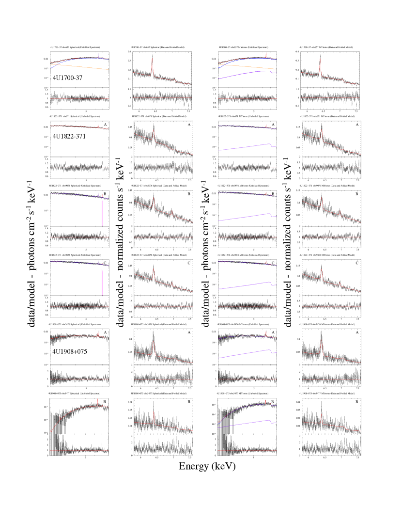

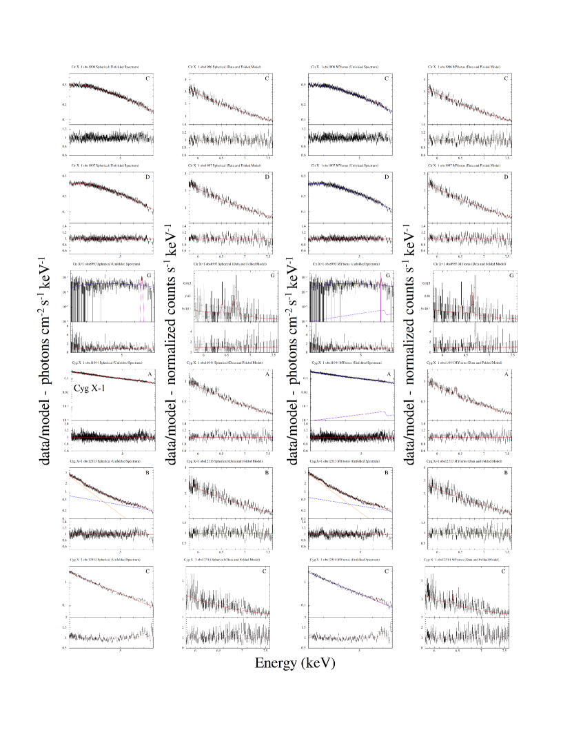
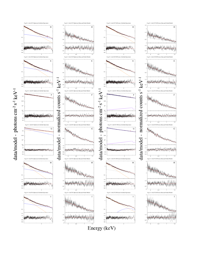
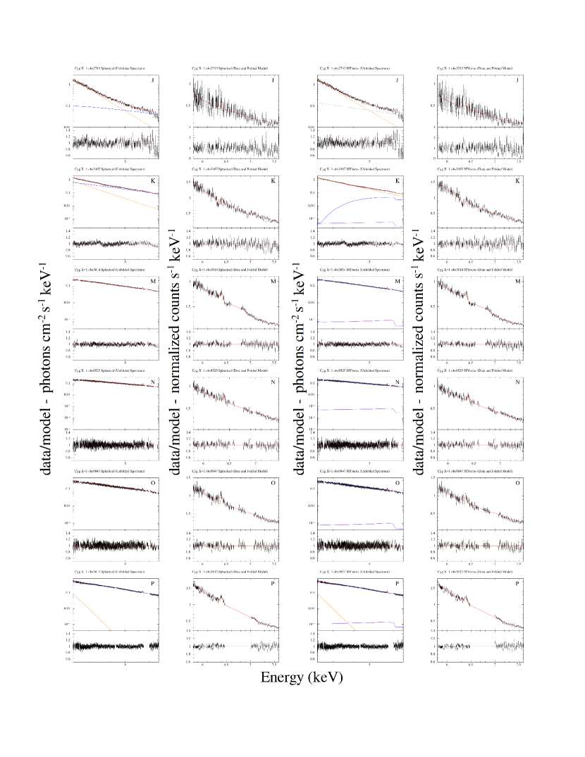
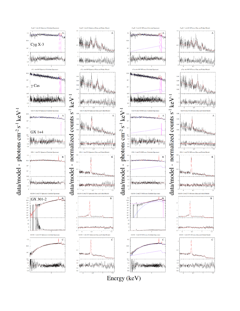

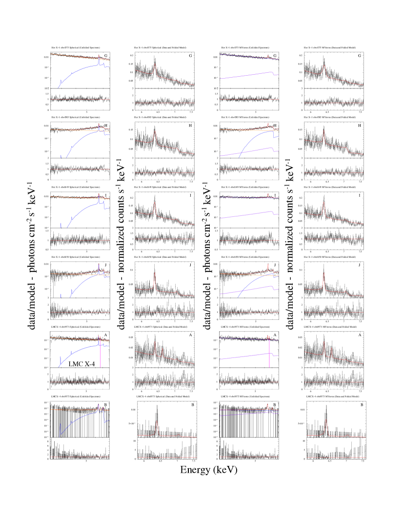
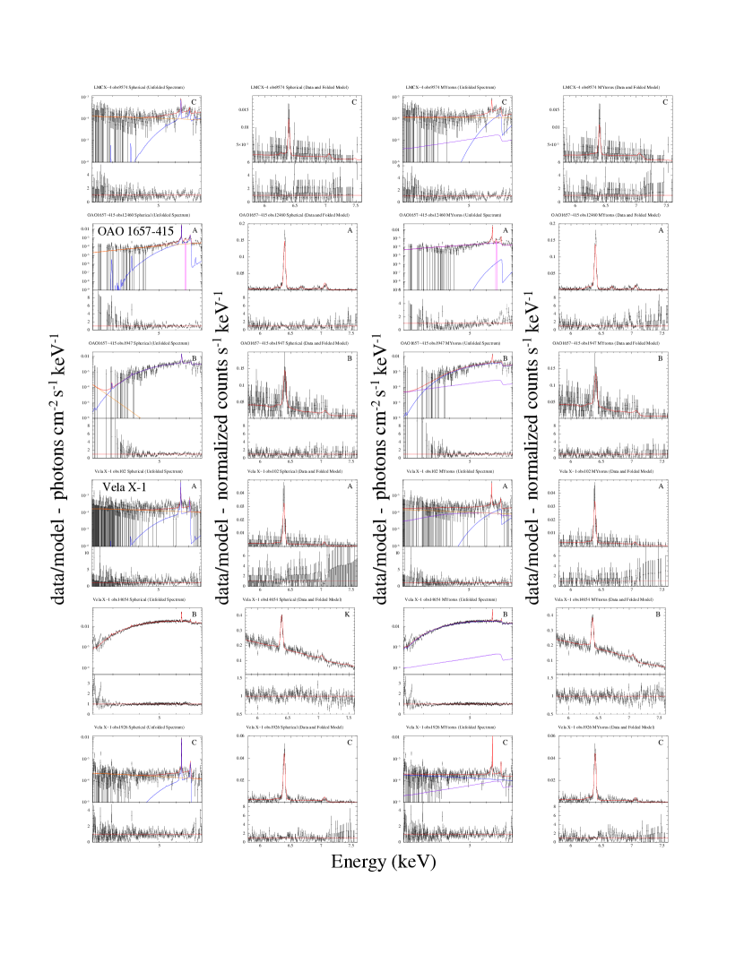
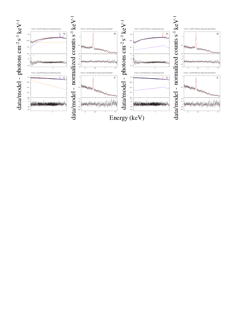
Appendix C
Contour plots of FWHM vs. N for Fe K detections.
We plot FWHM vs. contours for mytorus fits at join confidence levels corresponding to 68% (black curves), 90% (red curves), and 99% (blue curves).
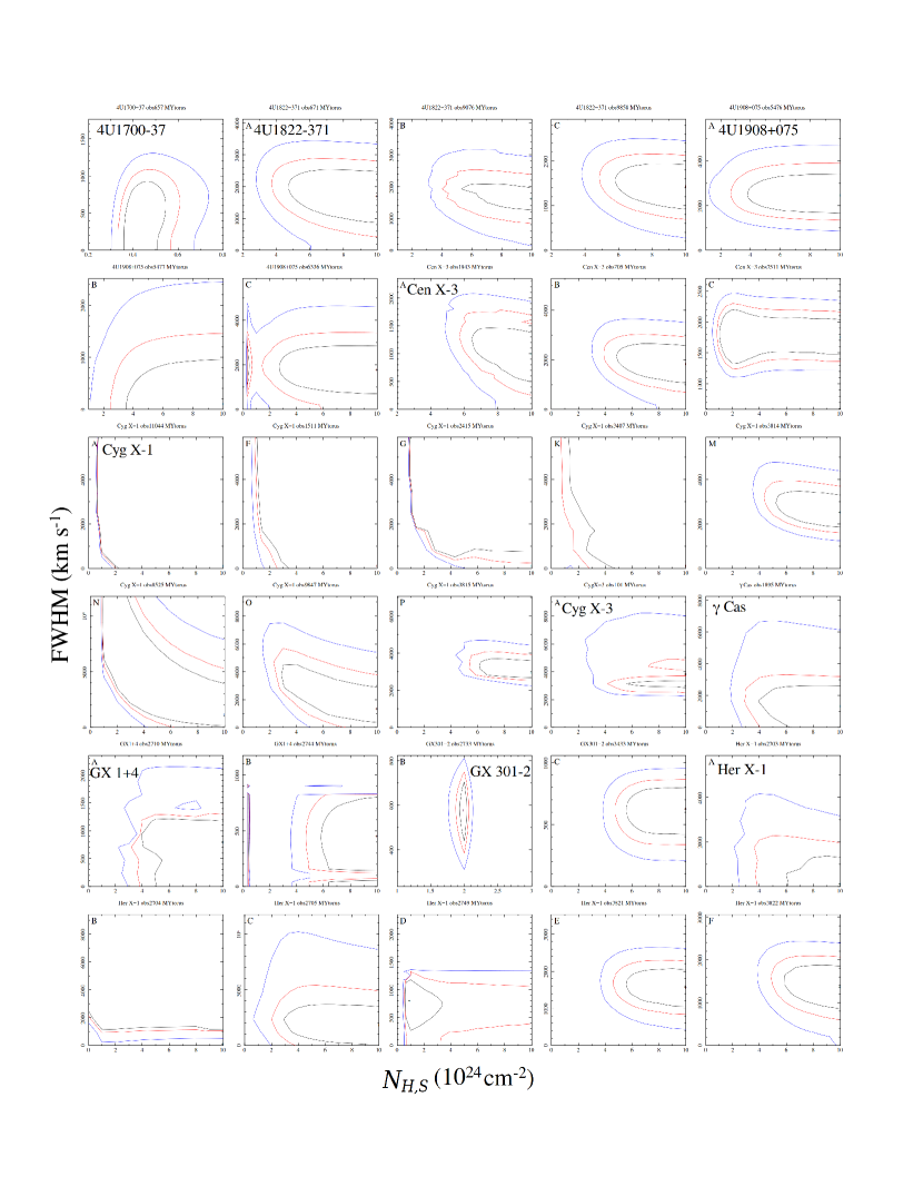
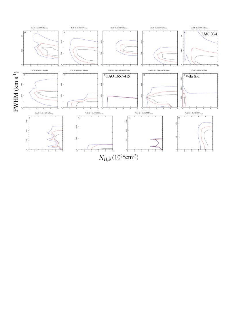
References
- Anders & Grevesse (1989) Anders, E., & Grevesse, N. 1989, Geochim. Cosmochim. Acta, 53, 197
- Anderson et al. (1994) Anderson, S. F., Wachter, S., Margon, B., et al. 1994, ApJ, 436, 319
- Arnaud (1996) Arnaud, K. A. 1996, in Astronomical Society of the Pacific Conference Series, Vol. 101, Astronomical Data Analysis Software and Systems V, ed. G. H. Jacoby & J. Barnes, 17
- Asai et al. (2014) Asai, K., Mihara, T., Matsuoka, M., et al. 2014, PASJ, 66, 79
- Asami et al. (2014) Asami, F., Enoto, T., Iwakiri, W., et al. 2014, PASJ, 66, 44
- Ash et al. (1999) Ash, T. D. C., Reynolds, A. P., Roche, P., et al. 1999, MNRAS, 307, 357
- Boroson et al. (2001) Boroson, B., Kallman, T., & Vrtilek, S. D. 2001, ApJ, 562, 925
- Boroson et al. (2003) Boroson, B., Vrtilek, S. D., Kallman, T., & Corcoran, M. 2003, ApJ, 592, 516
- Boutloukos et al. (2006) Boutloukos, S., van der Klis, M., Altamirano, D., et al. 2006, ApJ, 653, 1435
- Brandt & Schulz (2000) Brandt, W. N., & Schulz, N. S. 2000, ApJ, 544, L123
- Brightman & Nandra (2011) Brightman, M., & Nandra, K. 2011, MNRAS, 413, 1206
- Burderi et al. (2000) Burderi, L., Di Salvo, T., Robba, N. R., La Barbera, A., & Guainazzi, M. 2000, ApJ, 530, 429
- Canizares et al. (2005) Canizares, C. R., Davis, J. E., Dewey, D., et al. 2005, PASP, 117, 1144
- Chakrabarty et al. (2002) Chakrabarty, D., Wang, Z., Juett, A. M., Lee, J. C., & Roche, P. 2002, ApJ, 573, 789
- Clark et al. (2002) Clark, J. S., Goodwin, S. P., Crowther, P. A., et al. 2002, A&A, 392, 909
- Cottam et al. (2001) Cottam, J., Sako, M., Kahn, S. M., Paerels, F., & Liedahl, D. A. 2001, ApJ, 557, L101
- Duro et al. (2011) Duro, R., Dauser, T., Wilms, J., et al. 2011, A&A, 533, L3
- Duro et al. (2016) Duro, R., Dauser, T., Grinberg, V., et al. 2016, A&A, 589, A14
- Fabian et al. (2012) Fabian, A. C., Wilkins, D. R., Miller, J. M., et al. 2012, MNRAS, 424, 217
- Falanga et al. (2015) Falanga, M., Bozzo, E., Lutovinov, A., et al. 2015, A&A, 577, A130
- Farinelli et al. (2016) Farinelli, R., Ferrigno, C., Bozzo, E., & Becker, P. A. 2016, A&A, 591, A29
- Fridriksson et al. (2015) Fridriksson, J. K., Homan, J., & Remillard, R. A. 2015, ApJ, 809, 52
- Fürst et al. (2011) Fürst, F., Suchy, S., Kreykenbohm, I., et al. 2011, A&A, 535, A9
- Fürst et al. (2013) Fürst, F., Grefenstette, B. W., Staubert, R., et al. 2013, ApJ, 779, 69
- Goldstein et al. (2004) Goldstein, G., Huenemoerder, D. P., & Blank, D. 2004, AJ, 127, 2310
- Gottwald et al. (1995) Gottwald, M., Parmar, A. N., Reynolds, A. P., et al. 1995, A&AS, 109, 9
- Gou et al. (2011) Gou, L., McClintock, J. E., Reid, M. J., et al. 2011, ApJ, 742, 85
- Gou et al. (2014) Gou, L., McClintock, J. E., Remillard, R. A., et al. 2014, ApJ, 790, 29
- Grinberg et al. (2013) Grinberg, V., Hell, N., Pottschmidt, K., et al. 2013, A&A, 554, A88
- Hanson et al. (2000) Hanson, M. M., Still, M. D., & Fender, R. P. 2000, ApJ, 541, 308
- Harmanec et al. (2000) Harmanec, P., Habuda, P., Štefl, S., et al. 2000, A&A, 364, L85
- Heemskerk & van Paradijs (1989) Heemskerk, M. H. M., & van Paradijs, J. 1989, A&A, 223, 154
- Herrero et al. (1995) Herrero, A., Kudritzki, R. P., Gabler, R., Vilchez, J. M., & Gabler, A. 1995, A&A, 297, 556
- Hinkle et al. (2006) Hinkle, K. H., Fekel, F. C., Joyce, R. R., et al. 2006, ApJ, 641, 479
- Huenemoerder et al. (2011) Huenemoerder, D. P., Mitschang, A., Dewey, D., et al. 2011, AJ, 141, 129
- Hung et al. (2010) Hung, L.-W., Hickox, R. C., Boroson, B. S., & Vrtilek, S. D. 2010, ApJ, 720, 1202
- Iaria et al. (2013) Iaria, R., Di Salvo, T., D’Aì, A., et al. 2013, A&A, 549, A33
- Iaria et al. (2005) Iaria, R., Di Salvo, T., Robba, N. R., et al. 2005, ApJ, 634, L161
- Iaria et al. (2015) Iaria, R., Di Salvo, T., Matranga, M., et al. 2015, A&A, 577, A63
- Islam & Paul (2014) Islam, N., & Paul, B. 2014, MNRAS, 441, 2539
- Jaisawal & Naik (2014) Jaisawal, G. K., & Naik, S. 2014, Bulletin of the Astronomical Society of India, 42, 147
- Jaisawal & Naik (2015) —. 2015, MNRAS, 448, 620
- Ji et al. (2009) Ji, L., Schulz, N., Nowak, M., Marshall, H. L., & Kallman, T. 2009, ApJ, 700, 977
- Ji et al. (2011) Ji, L., Schulz, N. S., Nowak, M. A., & Canizares, C. R. 2011, ApJ, 729, 102
- Jimenez-Garate et al. (2005) Jimenez-Garate, M. A., Raymond, J. C., Liedahl, D. A., & Hailey, C. J. 2005, ApJ, 625, 931
- Johnston et al. (1999) Johnston, H. M., Fender, R., & Wu, K. 1999, MNRAS, 308, 415
- Jonker et al. (2007) Jonker, P. G., Nelemans, G., & Bassa, C. G. 2007, MNRAS, 374, 999
- Jonker et al. (2003) Jonker, P. G., van der Klis, M., & Groot, P. J. 2003, MNRAS, 339, 663
- Kalberla et al. (2005) Kalberla, P. M. W., Burton, W. B., Hartmann, D., et al. 2005, A&A, 440, 775
- Kallman et al. (2004) Kallman, T. R., Palmeri, P., Bautista, M. A., Mendoza, C., & Krolik, J. H. 2004, ApJS, 155, 675
- Kaper et al. (2006) Kaper, L., van der Meer, A., & Najarro, F. 2006, A&A, 457, 595
- Kreykenbohm et al. (2008) Kreykenbohm, I., Wilms, J., Kretschmar, P., et al. 2008, A&A, 492, 511
- LaMassa et al. (2014) LaMassa, S. M., Yaqoob, T., Ptak, A. F., et al. 2014, ApJ, 787, 61
- Lang et al. (1981) Lang, F. L., Levine, A. M., Bautz, M., et al. 1981, ApJ, 246, L21
- Leahy & Abdallah (2014) Leahy, D. A., & Abdallah, M. H. 2014, ApJ, 793, 79
- Leahy & Kostka (2008) Leahy, D. A., & Kostka, M. 2008, MNRAS, 384, 747
- Levine et al. (2004) Levine, A. M., Rappaport, S., Remillard, R., & Savcheva, A. 2004, ApJ, 617, 1284
- Linares et al. (2010) Linares, M., Watts, A., Altamirano, D., et al. 2010, ApJ, 719, L84
- Liu & Li (2014) Liu, Y., & Li, X. 2014, ApJ, 787, 52
- Madsen et al. (2017) Madsen, K. K., Beardmore, A. P., Forster, K., et al. 2017, AJ, 153, 2
- Maitra & Paul (2013) Maitra, C., & Paul, B. 2013, ApJ, 763, 79
- Manousakis et al. (2012) Manousakis, A., Walter, R., & Blondin, J. M. 2012, A&A, 547, A20
- Martínez-Núñez et al. (2015) Martínez-Núñez, S., Sander, A., Gímenez-García, A., et al. 2015, A&A, 578, A107
- Martínez-Núñez et al. (2014) Martínez-Núñez, S., Torrejón, J. M., Kühnel, M., et al. 2014, A&A, 563, A70
- Martins et al. (2007) Martins, F., Genzel, R., Hillier, D. J., et al. 2007, A&A, 468, 233
- Mason et al. (2012) Mason, A. B., Clark, J. S., Norton, A. J., et al. 2012, MNRAS, 422, 199
- Miller (2007) Miller, J. M. 2007, ARA&A, 45, 441
- Miller et al. (2012) Miller, J. M., Pooley, G. G., Fabian, A. C., et al. 2012, ApJ, 757, 11
- Miller et al. (2002) Miller, J. M., Fabian, A. C., Wijnands, R., et al. 2002, ApJ, 578, 348
- Miškovičová et al. (2016) Miškovičová, I., Hell, N., Hanke, M., et al. 2016, A&A, 590, A114
- Morel & Grosdidier (2005) Morel, T., & Grosdidier, Y. 2005, MNRAS, 356, 665
- Motta et al. (2017) Motta, S. E., Kajava, J. J. E., Sánchez-Fernández, C., Giustini, M., & Kuulkers, E. 2017, MNRAS, 468, 981
- Muñoz-Darias et al. (2005) Muñoz-Darias, T., Casares, J., & Martínez-Pais, I. G. 2005, ApJ, 635, 502
- Mukherjee & Paul (2004) Mukherjee, U., & Paul, B. 2004, A&A, 427, 567
- Murphy & Yaqoob (2009) Murphy, K. D., & Yaqoob, T. 2009, MNRAS, 397, 1549
- Naik et al. (2011) Naik, S., Paul, B., & Ali, Z. 2011, ApJ, 737, 79
- Nandra et al. (2007) Nandra, K., O’Neill, P. M., George, I. M., & Reeves, J. N. 2007, MNRAS, 382, 194
- Neilsen et al. (2009) Neilsen, J., Lee, J. C., Nowak, M. A., Dennerl, K., & Vrtilek, S. D. 2009, ApJ, 696, 182
- Netzer et al. (1990) Netzer, H., Maoz, D., Laor, A., et al. 1990, ApJ, 353, 108
- Nowak et al. (2011) Nowak, M. A., Hanke, M., Trowbridge, S. N., et al. 2011, ApJ, 728, 13
- Oosterbroek et al. (2001) Oosterbroek, T., Parmar, A. N., Orlandini, M., et al. 2001, A&A, 375, 922
- Orosz et al. (2011) Orosz, J. A., McClintock, J. E., Aufdenberg, J. P., et al. 2011, ApJ, 742, 84
- Paerels et al. (2000) Paerels, F., Cottam, J., Sako, M., et al. 2000, ApJ, 533, L135
- Palmeri et al. (2003) Palmeri, P., Mendoza, C., Kallman, T. R., Bautista, M. A., & Meléndez, M. 2003, A&A, 410, 359
- Parker et al. (2015) Parker, M. L., Tomsick, J. A., Miller, J. M., et al. 2015, ApJ, 808, 9
- Paul et al. (2005) Paul, B., Dotani, T., Nagase, F., Mukherjee, U., & Naik, S. 2005, ApJ, 627, 915
- Pradhan et al. (2014) Pradhan, P., Maitra, C., Paul, B., Islam, N., & Paul, B. C. 2014, MNRAS, 442, 2691
- Quaintrell et al. (2003) Quaintrell, H., Norton, A. J., Ash, T. D. C., et al. 2003, A&A, 401, 313
- Rawls et al. (2011) Rawls, M. L., Orosz, J. A., McClintock, J. E., et al. 2011, ApJ, 730, 25
- Reynolds et al. (1997) Reynolds, A. P., Quaintrell, H., Still, M. D., et al. 1997, MNRAS, 288, 43
- Reynolds (2014) Reynolds, C. S. 2014, Space Sci. Rev., 183, 277
- Reynolds (2016) —. 2016, Astron. Nach., 337, 404
- Sasano et al. (2014) Sasano, M., Makishima, K., Sakurai, S., Zhang, Z., & Enoto, T. 2014, PASJ, 66, 35
- Schulz & Brandt (2002) Schulz, N. S., & Brandt, W. N. 2002, ApJ, 572, 971
- Schulz et al. (2002) Schulz, N. S., Canizares, C. R., Lee, J. C., & Sako, M. 2002, ApJ, 564, L21
- Schulz et al. (2016) Schulz, N. S., Corrales, L., & Canizares, C. R. 2016, ApJ, 827, 49
- Shtykovsky et al. (2017) Shtykovsky, A. E., Lutovinov, A. A., Arefiev, V. A., et al. 2017, \anl, 43, 175
- Shu et al. (2011) Shu, X. W., Yaqoob, T., & Wang, J. X. 2011, ApJ, 738, 147
- Smith et al. (2004) Smith, M. A., Cohen, D. H., Gu, M. F., et al. 2004, ApJ, 600, 972
- Smith et al. (2012) Smith, M. A., Lopes de Oliveira, R., Motch, C., et al. 2012, A&A, 540, A53
- Stark & Saia (2003) Stark, M. J., & Saia, M. 2003, ApJ, 587, L101
- Stella & Vietri (1999) Stella, L., & Vietri, M. 1999, Physical Review Letters, 82, 17
- Suchy et al. (2012) Suchy, S., Fürst, F., Pottschmidt, K., et al. 2012, ApJ, 745, 124
- Tennant et al. (1986) Tennant, A. F., Fabian, A. C., & Shafer, R. A. 1986, MNRAS, 219, 871
- Thorsett & Chakrabarty (1999) Thorsett, S. E., & Chakrabarty, D. 1999, ApJ, 512, 288
- Tomsick et al. (2014) Tomsick, J. A., Nowak, M. A., Parker, M., et al. 2014, ApJ, 780, 78
- Torrejón et al. (2010) Torrejón, J. M., Schulz, N. S., Nowak, M. A., & Kallman, T. R. 2010, ApJ, 715, 947, (T10)
- Tsujimoto et al. (2011) Tsujimoto, M., Guainazzi, M., Plucinsky, P. P., et al. 2011, A&A, 525, A25
- van der Meer et al. (2005) van der Meer, A., Kaper, L., di Salvo, T., et al. 2005, A&A, 432, 999
- van der Meer et al. (2007) van der Meer, A., Kaper, L., van Kerkwijk, M. H., Heemskerk, M. H. M., & van den Heuvel, E. P. J. 2007, A&A, 473, 523
- Verner et al. (1996) Verner, D. A., Ferland, G. J., Korista, K. T., & Yakovlev, D. G. 1996, ApJ, 465, 487
- Vilhu et al. (2009) Vilhu, O., Hakala, P., Hannikainen, D. C., McCollough, M., & Koljonen, K. 2009, A&A, 501, 679
- Walton et al. (2016) Walton, D. J., Tomsick, J. A., Madsen, K. K., et al. 2016, ApJ, 826, 87
- Watanabe et al. (2003) Watanabe, S., Sako, M., Ishida, M., et al. 2003, ApJ, 597, L37
- Watanabe et al. (2006) —. 2006, ApJ, 651, 421
- White & Holt (1982) White, N. E., & Holt, S. S. 1982, ApJ, 257, 318
- Wojdowski et al. (2003) Wojdowski, P. S., Liedahl, D. A., Sako, M., Kahn, S. M., & Paerels, F. 2003, ApJ, 582, 959
- Wolff et al. (2016) Wolff, M. T., Becker, P. A., Gottlieb, A. M., et al. 2016, ApJ, 831, 194
- Yaqoob (2012) Yaqoob, T. 2012, MNRAS, 423, 3360
- Yaqoob et al. (2010) Yaqoob, T., Murphy, K. D., Miller, L., & Turner, T. J. 2010, MNRAS, 401, 411
- Yaqoob et al. (2015) Yaqoob, T., Tatum, M. M., Scholtes, A., Gottlieb, A., & Turner, T. J. 2015, MNRAS, 454, 973
- Yaqoob et al. (2016) Yaqoob, T., Turner, T. J., Tatum, M. M., Trevor, M., & Scholtes, A. 2016, MNRAS, 462, 4038
- Yoshida et al. (2017) Yoshida, Y., Kitamoto, S., Suzuki, H., et al. 2017, ApJ, 838, 30
- Zane et al. (2004) Zane, S., Ramsay, G., Jimenez-Garate, M. A., Willem den Herder, J., & Hailey, C. J. 2004, MNRAS, 350, 506