Fourier domain gravitational waveforms for precessing eccentric binaries

Abstract

We build two families of inspiral waveforms for precessing binaries on eccentric orbits in the Fourier domain. To achieve this, we use a small eccentricity expansion of the waveform amplitudes in order to separate the periastron precession timescale from the orbital timescale, and use a shifted uniform asymptotics transformation to compute the Fourier transform in the presence of spin-induced precession. We show that the resulting waveforms can yield a median faithfulness above 0.993 when compared to an equivalent time domain waveform with an initial eccentricity of $e_{0}\approx 0.3$. We also show that when the spins are large, using a circular waveform can potentially lead to significant biases in the recovery of the parameters, even when the system has fully circularized, particularly when the accumulated number of cycles is large. This is an effect of the residual eccentricity present when the objects forming the binary have nonvanishing spin components in the orbital plane.

I Introduction

The recent discoveries of gravitational wave (GW) signals by the LIGO and Virgo Collaborations have opened a new observation window on the Universe Aasi et al. (2015); Accadia et al. (2012); Grote and LIGO Scientific Collaboration (2010); Abbott et al. (2016a, b, 2017a, 2017b, 2017c, 2017d), through which the potential for new discoveries in astrophysics is truly tremendous. So far, those events have been analyzed with the assumption that the systems that produced them were evolving on circular orbits. Indeed, it has been a well-known fact that the emission of gravitational waves by binary systems has the tendency to circularize their orbits Peters (1964). Nevertheless, it has been argued that certain astrophysical scenarios could lead to stellar-origin black holes binaries having high initial eccentricities Postnov and Yungelson (2014); Shappee and Thompson (2013); Antonini et al. (2016, 2017), so they would still be measurable when the signal reaches the frequency window of the space-based GW detector LISA Nishizawa et al. (2016, 2017); Breivik et al. (2016). Furthermore, recent results have shown that eccentricity measurements by LIGO could be used to constrain stellar-mass black hole formation mechanisms Antonini et al. (2017); Petrovich and Antonini (2017); Samsing et al. (2018); Rodriguez et al. (2018); Hoang et al. (2018); Samsing et al. (2018). It has been estimated that large biases in the recovery of the parameters of the first direct detection GW150914 could have occurred if the initial eccentricity in the detector was $e_{0}\gtrsim 0.05$ Abbott et al. (2017e) Supermassive black hole binaries could also have important eccentricities in the late inspiral, if triple systems are a significant ingredient of supermassive black hole evolution Blaes et al. (2002); Hoffman and Loeb (2007); Amaro-Seoane et al. (2010); Bonetti et al. (2017, 2018a, 2018b). Furthermore, in some spin configurations, it has been shown that the eccentricity of the system never truly vanishes, but reaches a stationary value where it ceases to decrease through the emission of GWs Klein and Jetzer (2010).

This has motivated the development of waveforms that include the effects of a nonzero eccentricity in GW binary signals. The first steps towards this goal rely on the derivation of quasi-Keplerian equations describing the orbits Memmesheimer et al. (2004), the derivation of the evolution equations for the orbital elements Damour et al. (2004); Königsdörffer and Gopakumar (2006); Arun et al. (2008a, b, 2009), and the derivation of GW polarization amplitudes Mishra et al. (2015). The effects of individual spins were later added to this approach Gergely et al. (1998); Gergely (1999); Gergely and Keresztes (2003); Mikóczi et al. (2005); Keresztes et al. (2005); Klein and Jetzer (2010). Using these solutions, several waveforms have been developed. Yunes et al. Yunes et al. (2009) proposed an analytic eccentric waveform in the post-Newtonian (PN) postcircular approximation, by solving for the Fourier phase of a binary signal analytically at Newtonian order using a small eccentricity expansion. Cornish and Key Cornish and Key (2010, 2011); Key and Cornish (2011) and Gopakumar and Schäfer Gopakumar and Schäfer (2011) independently developed a numerical waveform in the time domain by solving the 1.5PN equations of motion numerically together with the spin-orbit precession equations, and using 1.5PN accurate amplitudes. Huerta et al. Huerta et al. (2014) expanded the analytical work of Yunes et al. by including the most important eccentricity-dependent terms up to 3.5PN order and at eighth order in the initial eccentricity for non-spinning systems. Tanay et al. Tanay et al. (2016) later computed the full 2PN Fourier phase for nonspinning systems at second order in the eccentricity. Moore et al. Moore et al. (2016) then expanded this result to 3PN order. Huerta et al. Huerta et al. (2017, 2018) and Hinder et al. Hinder et al. (2018) combined those results with numerical relativity to produce an eccentric inspiral-merger-ringdown waveform for nonspinning binaries. Recently, Hinderer and Babak Hinderer and Babak (2017) and Cao and Han Cao and Han (2017) developed an eccentric waveform using a new approach in the effective one-body (EOB) formalism.

In this work, we further develop the formalism of post-Newtonian eccentric waveforms to include the effects of spin-induced precession in the Fourier domain. The advantage of Fourier domain waveforms over time domain ones is that they provide a much more computationally efficient way of computing a GW signal. Indeed, in order to produce a time domain waveform, one has to compute an equally spaced time series of the signal before computing its Fourier transform to use in detection or parameter estimation algorithms. The relevant timescale for this time series is the inverse of the maximum orbital frequency, which, being very short, makes this process computationally very expensive. Having a waveform available directly in the Fourier domain circumvents this problem and greatly reduces the computational cost of GW data analysis. In order to construct such a waveform, we solve the evolution equations for the orbital elements together with the orbit-averaged spin precession equations numerically at 3PN order, including spin effects at 2PN order. Using a quasi-Keplerian description of the orbit, we employ instantaneous nonspinning amplitudes to construct the resulting GW polarizations. We then use a shifted uniform asymptotics (SUA) technique Klein et al. (2014) to compute the waveforms in the Fourier domain. The resulting waveform has the advantage that the phasing is computed without any expansion for small eccentricities and thus can be be very faithful compared to corresponding time domain waveforms for moderate to large eccentricities ($e\lesssim 0.4$). However, the amplitudes require a small-eccentricity expansion, and thus we do not expect the present waveforms to be faithful for arbitrarily large eccentricities.

In Sec. II, we derive two different families of eccentric waveforms. Due to the similarity between the orbital timescale and the periastron-to-periastron timescale, we derive the first family by expanding the Fourier domain waveform into combined harmonics of the mean orbital phase and of the mean anomaly. We then derive the second family by further expanding the resulting Fourier phase and time-frequency relations for small differences between the two similar phases. In Sec. III, we describe simulations that we performed to compute the faithfulness between our Fourier domain waveforms and a corresponding time domain waveform, including a detailed summary of how these different waveforms are constructed. We also compare a circular waveform to probe which domain of the parameter space allows for such circular waveforms to be effectively used for parameter estimation of binary signals. We give concluding remarks in Sec. IV. Throughout this paper, we use geometric units where $G=c=1$.

II Waveform

In the presence of spins, the orbit of a binary system is, in general, not restricted to an orbital plane Barker and O’Connell (1975). Indeed, interactions between the spins and the orbit cause them to precess. However, in the post-Newtonian regime, the timescale on which this precession occurs is well separated from the other timescales present in the problem. We can therefore approximate the spin-orbital precession to be occurring much more slowly than the orbit, which allows us to describe it using a so-called quasi-Keplerian parametrization inside an orbital plane that stays perpendicular to the orbital angular momentum as the latter precesses. A quasi-Keplerian parametrization of the orbit of a spinning binary system is known at 3PN order for the nonspinning part Memmesheimer et al. (2004); Königsdörffer and Gopakumar (2006), and at 2PN order for the spin-dependent part Klein and Jetzer (2010). In this work, we restrict the quasi-Keplerian orbital description at 2PN for the computation of the polarization amplitudes. We can express the orbit at 2PN order as

$$r =a(1-e_{r}\cos u)+f_{r}(v)\,,$$ (1a)

$$\phi =(1+k)v+f_{\phi}(v)\,,$$ (1b)

$$\tan\frac{v}{2} =\sqrt{\frac{1+e_{\phi}}{1-e_{\phi}}}\tan\frac{u}{2}\,,$$ (1c)

$$l =u-e_{t}\sin u+f_{t}(u,v)\,,$$ (1d)

$$\dot{l} =n\,,$$ (1e)

where $(r,\phi)$ is a polar representation of the separation vector in the orbital plane, $a$ is the semimajor axis; $u$ is the eccentric anomaly; $v$ is the true anomaly; $l$ is the mean anomaly; $n$ is the mean motion; $e_{r}$, $e_{\phi}$ and $e_{t}$ are eccentricity parameters; and the functions $f_{i}$ are general relativistic corrections given by Memmesheimer et al. (2004); Damour et al. (2004); Klein and Jetzer (2010)

$$f_{r}(v)= \;\sum_{i=0}^{2}b_{r,i}\cos(2v-2\psi_{i})\,,$$ (2a)

$$f_{\phi}(v)= \;\sum_{k=2}^{3}a_{\phi,k}\sin(kv)$$

$$+\sum_{k=1}^{2}\sum_{i=0}^{2}b_{\phi,k,i}\sin(kv-2\psi_{i})\,,$$ (2b)

$$f_{t}(u,v)= \;g_{t}(v-u)+a_{t}\sin(v)\,,$$ (2c)

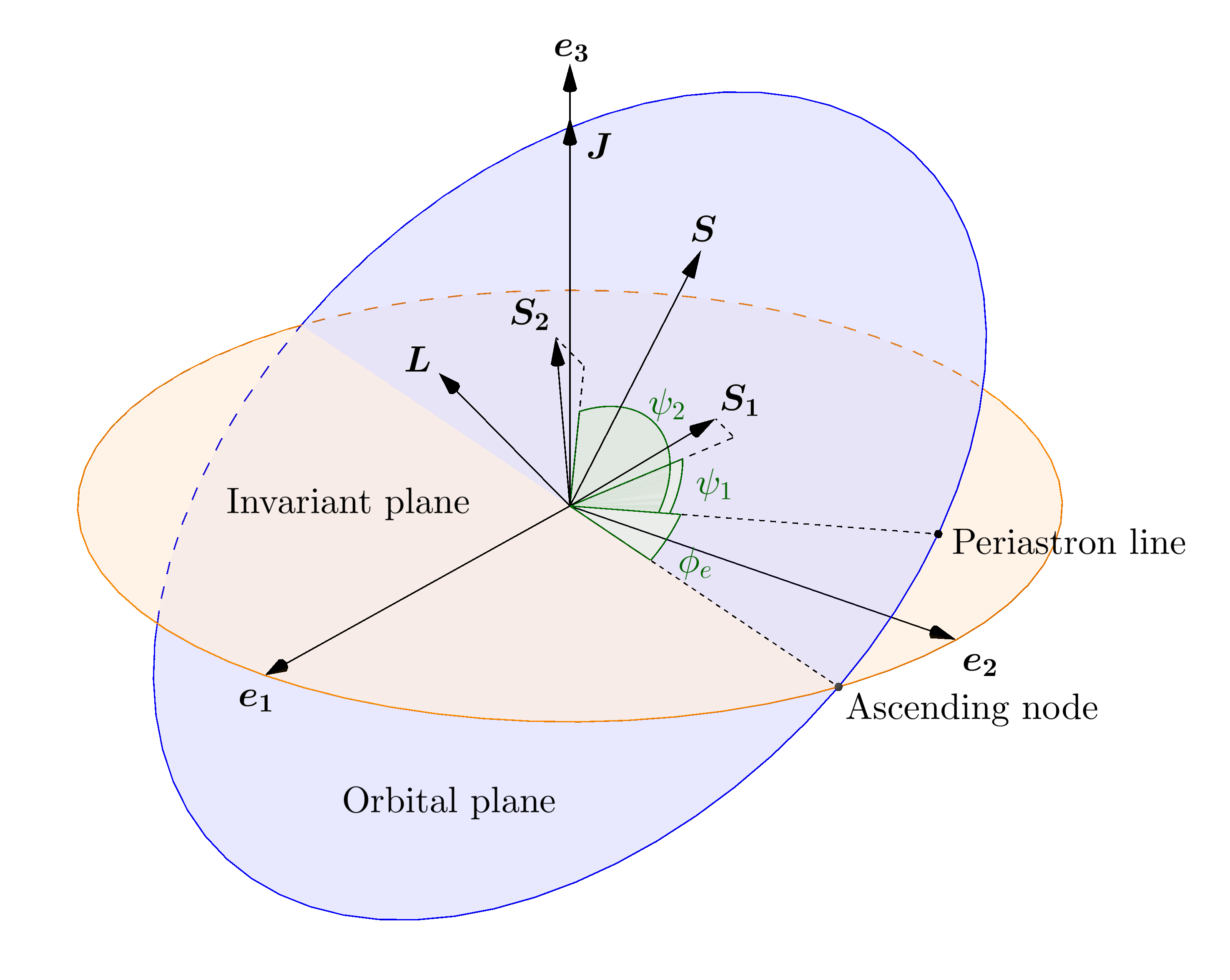
where $\psi_{i}$ is the angle between the periastron line and the projection of spin $i$ onto the orbital plane (see Fig. 1), $\psi_{0}=(\psi_{1}+\psi_{2})/2$ and the constants $a_{A}$, $b_{A}$ and $g_{t}$ are listed in Appendix B. We complemented the spinning solution of  Klein and Jetzer (2010) by including quadrupole-monopole terms as described in Appendix  A.

Figure 1: Angles used in the definition of the relativistic corrections defined in Eq. (2). The orbital plane is perpendicular to the Newtonian orbital angular momentum $\bm{L}$, and the invariant plane is perpendicular to the conserved total angular momentum $\bm{J}$. The angle $\phi_{e}$ locates the periastron line with respect to the fixed invariant plane, and the angles $\psi_{i}$ are subtended by the periastron line and the projections of the spins onto the orbital plane.

The orbital phase $\phi$ and the mean anomaly $l$ can be decomposed as the sum of a linearly growing part and a periodic part Damour et al. (2004),

$$\phi =\lambda+W_{\phi}\,,$$ (3a)

$$\dot{\lambda} =(1+k)n\,,$$ (3b)

$$\dot{l} =n\,,$$ (3c)

$$W_{\phi} =(1+k)(v-l)+f_{\phi}(v)\,.$$ (3d)

We choose to express our equations in terms of the post-Newtonian parameter $y$ and the eccentricity parameter $e$ defined by

$$y =\frac{\left[M(1+k)n\right]^{1/3}}{\sqrt{1-e_{t}^{2}}}\,,$$ (4a)

$$e =e_{t}\,.$$ (4b)

The constants in the quasi-Keplerian parametrization are given in terms of these parameters in Appendix B.

As the system emits gravitational waves, the orbital frequency and the eccentricity will evolve according to the following equations Damour et al. (2004); Klein and Jetzer (2010)

$$M\frac{dy}{dt} =\left(1-e^{2}\right)^{3/2}\nu y^{9}\left(a_{0}+\sum_{n=2}a_{n}y^{n}\right)\,,$$ (5a)

$$M\frac{de^{2}}{dt} =-\left(1-e^{2}\right)^{3/2}\nu y^{8}\left(b_{0}+\sum_{n=2}b_{n}y^{n}\right)\,,$$ (5b)

where the constants $a_{i}$ and $b_{i}$ are given at 3PN order for nonspinning systems and at 2PN order for spinning systems in Appendix C. Here we also complemented the spinning solution of Klein and Jetzer (2010) by including quadrupole-monopole terms as described in Appendix A. We found that the minimum value for the eccentricity $e^{2}_{\text{min}}$ found in Klein and Jetzer (2010) is unchanged by the addition of quadrupole-monopole effects, with

$$e^{2}_{\text{min}} =\frac{5y^{4}}{304}\sigma(-1,1,0,2,-2,0)$$

$$=\frac{5y^{4}}{304}\left|\bm{s}_{\perp}^{(-)}\right|^{2}\,,$$ (6)

where the 2PN spin-spin coupling $\sigma$ can be found in Appendix A, and

$$\bm{s}_{\perp}^{(-)} =\left[\bm{s}_{1}-\bm{\hat{L}}\left(\bm{\hat{L}}\cdot\bm{s}_{1}\right)\right]-\left[\bm{s}_{2}-\bm{\hat{L}}\left(\bm{\hat{L}}\cdot\bm{s}_{2}\right)\right],$$ (7)

where $\bm{\hat{L}}$ is a normal to the orbital plane.

Note that we found a typo in Klein and Jetzer (2010), where the constant factor in $e^{2}_{\text{min}}$ should read $5/304$ instead of $5/340$. This minimum eccentricity depends on the spin orientations: it is maximal when the spins lie inside the orbital plane and are opposite to one another, and it vanishes when the projections of $\bm{s}_{1}$ and $\bm{s}_{2}$ onto the orbital plane are equal to each other. The maximum value it can take is independent of the mass ratio; it is $e^{2}_{\text{min}}=5y^{4}/304$, which evaluates to $e_{\text{min}}\approx 0.021$ at the ISCO defined by $y=6^{-1/2}$, and it is multiplied by a factor $(f/f_{\text{ISCO}})^{2/3}$ earlier in the inspiral. Note that this minimum eccentricity, being a spin effect, is unrelated to a similar effect observed in extreme mass-ratio inspirals around Schwarzschild black holes in Cutler et al. (1994), and also unrelated to another effect due to orbital effects derived in Loutrel et al. (2018), which is of order $e^{2}_{\text{min}}\sim y^{10}$ and is independent of the spins.

The 2PN orbit-averaged equations of precession are given by Barker and O’Connell (1975); Racine (2008)

$$M\dot{\bm{\hat{L}}} =-\left(1-e^{2}\right)^{3/2}y^{6}\left(\bm{\Omega}_{1}+\bm{\Omega}_{2}\right)\,,$$ (8a)

$$M\dot{\bm{s}}_{1} =\left(1-e^{2}\right)^{3/2}\mu_{2}y^{5}\bm{\Omega}_{1}\,,$$ (8b)

$$M\dot{\bm{s}}_{2} =\left(1-e^{2}\right)^{3/2}\mu_{1}y^{5}\bm{\Omega}_{2}\,,$$ (8c)

where we defined the reduced spins $\bm{s}_{i}=\bm{S}_{i}/m_{i}$, the reduced individual masses $\mu_{i}=m_{i}/M$, and the precession vectors $\bm{\Omega}_{i}$ are given by

$$\bm{\Omega}_{i}= \;\bigg{\{}\left[2\mu_{i}+\frac{3}{2}\mu_{j}-\frac{3}{2}y\bm{\hat{L}}\cdot\left(\bm{s}+(q_{i}-1)\bm{s}_{i}\right)\right]\bm{\hat{L}}$$

$$+\frac{1}{2}y\bm{s}_{j}\bigg{\}}\times\bm{s}_{i}\,,$$ (9)

where $i,j\in\{1,2\}$, $i\neq j$, and the $q_{i}$ are quadrupole parameters defined in such a way that $q_{i}=1$ for black holes.

The gravitational waveform emitted by a binary system on such an orbit has been computed at 3PN order for nonspinning binaries, omitting tail effects Mishra et al. (2015). The result has the following structure:

$$h(t)= \;F_{+}(t)h_{+}(t)+F_{\times}(t)h_{\times}(t)\,,$$ (10a)

$$h_{+,\times}(t)= \;\sum_{n\in\mathbb{Z}}H_{+,\times}^{(n)}(y,e,e\cos u,e\sin u)e^{in(\phi+\phi_{T})}\,,$$ (10b)

where $F_{+}$ and $F_{\times}$ are antenna pattern functions Cutler (1998), and the Thomas precession phase $\phi_{T}$ is given by Apostolatos et al. (1994)

$$\dot{\phi}_{T} =\frac{\bm{\hat{L}}\cdot\bm{\hat{N}}}{1-\left(\bm{\hat{L}}\cdot\bm{\hat{N}}\right)^{2}}\left(\bm{\hat{L}}\times\bm{\hat{N}}\right)\cdot\dot{\bm{\hat{L}}}\,,$$ (11)

with respect to a given sky location vector $\bm{\hat{N}}$.

In order to compute the Fourier transform of this signal, we need to separate the orbital timescale from the precessional one, and express the orbital timescale dependence in terms of linearly growing phases. To do so, we follow Boetzel et al. (2017) and compute an inversion of the PN-accurate Kepler equation (1d) as

$$u =l+\sum_{s=1}^{\infty}A_{s}\sin(sl)\,,$$ (12)

with the Fourier coefficients $A_{s}$ given by

$$A_{s} =\frac{2}{s}J_{s}(se)+\sum_{j=1}^{\infty}\alpha_{j}\left[J_{s+j}(se)-J_{s-j}(se)\right]\,.$$ (13)

The PN-accurate constants $\alpha_{j}$ can be computed from Memmesheimer et al. (2004) and are given in Eq. (18) of Boetzel et al. (2017). Similarly, we can find a Fourier expansion of the true anomaly $v$ and the orbital phase $\phi$ in terms of the mean anomaly $l$:

$$v =l+\sum_{s=1}^{\infty}B_{s}\sin(sl)\,,$$ (14a)

$$\phi =\lambda+\sum_{s=1}^{\infty}C_{s}\sin(sl)\,.$$ (14b)

The Fourier coefficients $A_{s}$, $B_{s}$ and $C_{s}$ can be found up to $\mathcal{O}\left(y^{4},e^{5}\right)$ in Appendix D. Using this solution, we can then express

$$e^{iku} =\sum_{p\in\mathbb{Z}}\epsilon_{p}^{ku}\;e^{-ipl}\,,$$ (15a)

$$e^{ikv} =\sum_{p\in\mathbb{Z}}\epsilon_{p}^{kv}\;e^{-ipl}\,,$$ (15b)

$$e^{ik\phi} =e^{ik\lambda}\sum_{s\in\mathbb{Z}}\mathcal{P}_{p}^{k\phi}\;e^{-ipl}\,,$$ (15c)

where the coefficients $\epsilon_{p}^{ku}$, $\epsilon_{p}^{kv}$ and $\mathcal{P}_{p}^{k\phi}$ are given as a Taylor expansion in both $e$ and $y$. We refer to Eqs. (30), (34), (E11) of Boetzel et al. (2017) for how to calculate these Fourier coefficients.

This small eccentricity expansion allows us to express the waveform as

$$h_{+,\times}(t) =\sum_{n\in\mathbb{Z}}\sum_{p\in\mathbb{Z}}H_{+,\times}^{(p,n)}e^{-i(n\lambda+pl)}\,,$$ (16)

where we included the Thomas phase $\phi_{T}$ into the amplitudes $H_{+,\times}^{(p,n)}$, which vary on the spin-precession timescale. To separate the periastron precession timescale from the orbital timescale, we define $\delta\lambda=\lambda-l$, such that

$$M\dot{\lambda} =\left(1-e^{2}\right)^{3/2}y^{3}\,,$$ (17a)

$$\delta\dot{\lambda} =\frac{k}{1+k}\dot{\lambda}\,.$$ (17b)

This new angle defines the periastron precession timescale, which is similar to the spin precession timescale since $\delta\dot{\lambda}/\dot{\lambda}=\mathcal{O}\left(y^{2}\right)$.

Using this, we can then further simplify the waveform with

$$h_{+,\times}(t) =\sum_{n\in\mathbb{Z}}H_{+,\times}^{(n)}e^{-in\lambda}\,,$$ (18a)

$$H_{+,\times}^{(n)} =\frac{M\nu y^{2}}{d_{L}}\sum_{m\in\mathbb{Z}}G_{+,\times}^{(m,n)}e^{-im\delta\lambda}e^{-i(n+m)\phi_{T}}\,.$$ (18b)

The amplitudes $G_{+,\times}^{(m,n)}$ are given in Appendix E at order $\mathcal{O}\left(y^{2},e\right)$ .

II.1 Fourier transform approximations

Before we compute an approximation of the Fourier transform of our signal, let us introduce two useful techniques.

Let us first assume that we have a signal of the form

$$h(t) =A(t)e^{-i\phi(t)}\,,$$ (19)

with $\dot{\phi}(t)$ a positive and monotonically increasing function of time, and that we want to compute its Fourier transform

$$\tilde{h}(f) =\int_{-\infty}^{\infty}h(t)e^{2\pi ift}dt\,.$$ (20)

The stationary phase approximation (SPA) of this Fourier transform consists in Taylor expanding the amplitude $A(t)$ and phase $\phi(t)$ around the stationary point $t_{0}$ defined by the relation

$$2\pi f =\dot{\phi}(t_{0})\,,$$ (21)

keeping only the constant term in the expansion of the amplitude and up to the quadratic order in the expansion of the phase. We get

$$h(t)\approx \;A(t_{0})\exp\bigg{\{}-i\bigg{[}\phi(t_{0})$$

$$+\dot{\phi}(t_{0})(t-t_{0})+\frac{1}{2}\ddot{\phi}(t_{0})(t-t_{0})^{2}\bigg{]}\bigg{\}}\,.$$ (22)

We can compute the Fourier transform of this approximate signal analytically, and we get

$$\tilde{h}(f) \approx\sqrt{\frac{2\pi}{|\ddot{\phi}(t_{0})|^{2}}}A(t_{0})e^{i(2\pi ft_{0}-\phi(t_{0})-\pi/4)}\,.$$ (23)

This approximation will be accurate if $|\dot{A}/A|\ll|\ddot{\phi}|^{1/2}$ around the stationary point, and if the quadratic approximation is accurate around the stationary point. For a formal derivation, see e.g. Bender and Orszag (1999).

Let us now suppose that our signal is of the form

$$h(t) =Ae^{-i[\phi_{C}+B\sin\beta]}\,,$$ (24)

with $\dot{A}/A=\mathcal{O}\left(y^{8}\right)$, $\dot{\phi}_{C}=\mathcal{O}\left(y^{3}\right)$, $B=\mathcal{O}\left(y\right)$, $\dot{\beta}=\mathcal{O}\left(y^{5}\right)$, and that each additional time derivative adds a factor $\mathcal{O}\left(y^{8}\right)$ to the various quantities present in the signal, with $y$ a small expansion parameter. This is the simplified form of a GW signal that we expect from a binary system undergoing spin-induced orbital precession, with $y$ being a PN expansion parameter. The SPA cannot be directly used in this case, because the two terms in the second time derivative of the signal phase

$$\ddot{\phi} =\ddot{\phi}_{C}-B\dot{\beta}^{2}\sin\beta+\mathcal{O}\left(y^{13}\right)$$ (25)

are of the same PN order and can cancel each other. The shifted uniform asymptotics (SUA) method Klein et al. (2014) offers an approximation of the Fourier transform of such a signal by first expanding the signal using Bessel functions as

$$h(t) =A\sum_{k}J_{k}(B)e^{-i(\phi_{C}+k\beta)}\,,$$ (26)

so its Fourier transform can be approximated by a series of SPA, since $\ddot{\beta}\ll\ddot{\phi}_{C}$. The Fourier transform then becomes

$$\tilde{h}(f)\approx \;\sum_{k}A\sqrt{\frac{2\pi}{\ddot{\phi}_{C}+k\ddot{\beta}}}$$

$$\times\exp\left[i\left(2\pi ft_{k}-\phi_{C}-k\beta-\frac{\pi}{4}\right)\right]\,,$$ (27)

where the various functions are evaluated for each $k\in\mathbb{Z}$ at the stationary time $t_{k}$ defined by

$$2\pi f =\dot{\phi}_{C}(t_{k})+k\dot{\beta}(t_{k})\,.$$ (28)

The different stationary times can be related to each other by Taylor expanding their defining equations around $t_{0}$ and solving for the difference order by order:

$$t_{k}-t_{0} =-\frac{k\dot{\beta}(t_{0})}{\ddot{\phi}_{C}(t_{0})}+\mathcal{O}\left(y^{-4}\right)\,.$$ (29)

By Taylor expanding Eq. (27) around $t_{0}$, and keeping only the leading PN order amplitude and the phase accurate to order $\mathcal{O}\left(y^{0}\right)$, we obtain

$$\tilde{h}(f)\approx \;\tilde{h}_{0}(f)\tilde{h}_{\text{corr}}(f)\,,$$ (30a)

$$\tilde{h}_{0}(f)= \;\sqrt{\frac{2\pi}{|\ddot{\phi}(t_{0})|^{2}}}A(t_{0})e^{i(2\pi ft_{0}-\phi_{C}(t_{0})-\pi/4)}\,,$$ (30b)

$$\tilde{h}_{\text{corr}}(f)= \;\sum_{k}J_{k}[B(t_{0})]\exp\left[-k\beta(t_{0})+\frac{1}{2}T^{2}k^{2}\dot{\beta}^{2}(t_{0})\right],$$ (30c)

$$T= \;\sqrt{\frac{1}{\ddot{\phi}_{C}(t_{0})}}\,.$$ (30d)

After some manipulation, we can resum the Bessel functions in $\tilde{h}_{\text{corr}}(f)$ as

$$\tilde{h}_{\text{corr}}(f) =\sum_{p\geq 0}\frac{\left(-iT^{2}\right)^{p}}{2^{p}p!}\partial_{t}^{2p}e^{-iB\sin\beta}\,,$$ (31)

where the functions are evaluated at $t=t_{0}$. Truncating this series at some order $p=k_{\text{max}}$ and using a stencil around $t_{0}$ to approximate the different order time derivatives, we obtain the SUA approximation

$$\tilde{h}_{\text{corr}}(f) \approx\sum_{k=-k_{\text{max}}}^{k_{\text{max}}}a_{k,k_{\text{max}}}e^{-iB\sin\beta(t_{0}+kT)}\,,$$ (32)

where the constants $a_{k,k_{\text{max}}}$ satisfy the following linear system of equations:

$$\sum_{k=1}^{k_{\text{max}}}a_{k,k_{\text{max}}}+\frac{1}{2}a_{0,k_{\text{max}}}=1\,,$$ (33a)

$$\sum_{k=1}^{k_{\text{max}}}a_{k,k_{\text{max}}}\frac{k^{2p}}{(2p)!}=\frac{(-i)^{p}}{2^{p}p!}\,,\quad p\in\{1,\ldots,k_{\text{max}}\}\,,$$ (33b)

$$a_{-k,k_{\text{max}}}=a_{k,k_{\text{max}}}\,.$$ (33c)

To summarize, if we are able to separate the spin-precessional timescale effects from a carrier phase $\phi_{C}$ that satisfies $\dot{\phi}_{C}>0$ and $\ddot{\phi}_{C}>0$ as

$$h(t) =A(t)e^{-i\phi_{C}(t)}\,,$$ (34)

where all spin-precessional timescale effects are included in $A(t)$, then we can write the SUA approximation of its Fourier transform:

$$\tilde{h}(f)= \;\sqrt{\frac{2\pi}{\ddot{\phi}_{C}}}e^{i(2\pi ft_{0}-\phi_{C}(t_{0})-\pi/4)}$$

$$\times\sum_{k=-k_{\text{max}}}^{k_{\text{max}}}a_{k,k_{\text{max}}}A(t_{0}+kT)\,,$$ (35)

with the constants $a_{k,k_{\text{max}}}$ satisfying the linear system of Eqs. (33), and $T=[\ddot{\phi}_{C}(t_{0})]^{-1/2}$.

II.2 Periastron precession effects

Let us first derive a waveform in the Fourier domain taht is valid for nonprecessing spins, and add the effects of spin-orbit precession later. Putting aside spin-orbit precession, the signal in the time domain can be expressed as in Eqs. (18):

$$h_{+,\times}(t) =\frac{M\nu y^{2}}{d_{L}}\sum_{n\in\mathbb{Z}}\sum_{m\in\mathbb{Z}}G_{+,\times}^{(m,n)}e^{-i(n\lambda+m\delta\lambda)}\,.$$ (36)

Using the SPA, we can approximate its Fourier transform by

$$\tilde{h}_{+,\times}(f)= \;\int h_{+,\times}(t)e^{2\pi ift}dt$$

$$= \;\frac{M\nu y^{2}}{d_{L}}\sum_{n\geq 1}\sum_{m\in\mathbb{Z}}\sqrt{\frac{2\pi}{n\ddot{\lambda}+m\delta\ddot{\lambda}}}G_{+,\times}^{(m,n)}$$

$$\times e^{i\left[2\pi ft_{n,m}-n\lambda(t_{n,m})-m\delta\lambda(t_{n,m})-\pi/4\right]}\,,$$ (37a)

$$2\pi f= \;n\dot{\lambda}(t_{n,m})+m\delta\dot{\lambda}(t_{n,m})\,,$$ (37b)

where each of the harmonics $(n,m)$ has to be evaluated at a different time. It is worth noting here that we assumed that $n\dot{\lambda}+m\delta\dot{\lambda}>0$, which is not necessarily true for every $(n,m)$ pair during the whole inspiral. However, for this assumption to break down, one needs negative and sufficiently large $m$, since $\delta\dot{\lambda}/\dot{\lambda}=\mathcal{O}\left(y^{2}\right)$, and the corresponding amplitude will be suppressed by a factor $e^{m}$. We verified that ignoring this fact does not lead to high inaccuracies, at least for initial eccentricities $e_{0}\lesssim 0.4$.

In order to simplify the expression of the Fourier domain waveform and to improve its computational efficiency, we look for an expression of the following form:

$$\tilde{h}_{+,\times}(f) =\frac{M\nu y^{2}}{d_{L}}\sum_{n\geq 1}\tilde{h}_{n,0}(f)\sum_{m\in\mathbb{Z}}\tilde{h}_{n,m}^{\text{PP}}(f)\,,$$ (38a)

$$\tilde{h}_{n,0}(f) =\sqrt{\frac{2\pi}{n\ddot{\lambda}}}e^{i[2\pi ft_{n}-n\lambda(t_{n})-\pi/4]}\,,$$ (38b)

$$2\pi f =n\dot{\lambda}(t_{n})\,,$$ (38c)

where $\tilde{h}_{n,0}(f)$ is a waveform harmonic without any periastron precession effects and $\tilde{h}_{n,m}^{\text{PP}}(f)$ are corrections to it. In order to evaluate $\tilde{h}_{n,m}^{\text{PP}}(f)$, we define

$$\Delta t_{n,m} =t_{n,m}-t_{n}\,,$$ (39)

and Taylor expand Eq. (37b) around $t_{n}$:

$$2\pi f =\sum_{p\geq 0}\frac{\Delta t_{n,m}^{p}}{p!}\left.\frac{d^{p}}{dt^{p}}\left(n\dot{\lambda}+m\delta\dot{\lambda}\right)\right|_{t=t_{n}}\,.$$ (40)

We can use this together with Eq. (38c) to solve for the PN expansion of $\Delta t_{n,m}$ order by order, and we obtain

$$\Delta t_{n,m} =\sum_{p=1}^{P}\frac{1}{p!}\left(-\frac{m}{n}\right)^{p}D^{p-1}\left(\frac{\delta\dot{\lambda}^{p}}{\ddot{\lambda}}\right)\,,$$ (41)

where the differential operator $D$ is given by

$$D =\frac{1}{\ddot{\lambda}}\frac{d}{dt}\,,$$ (42)

and every function of time is evaluated at $t=t_{n}$. We have checked that this expression remains valid at least up to $P=6$.

Using this, we can then Taylor expand the phase in Eq. (37a) around $t_{n}$ to compute

$$\tilde{h}_{n,m}^{\text{PP}}(f) =G_{+,\times}^{(m,n)}e^{i\Delta\Psi_{n,m}}\,,$$ (43a)

$$\Delta\Psi_{n,m} =-m\delta\lambda+n\sum_{p=2}^{P+1}\frac{1}{p!}\left(-\frac{m}{n}\right)^{p}D^{p-2}\left(\frac{\delta\dot{\lambda}^{p}}{\ddot{\lambda}}\right)\,,$$ (43b)

where all functions are once again evaluated at the stationary time $t_{n}$ defined by Eq. (38c), and we checked that the latter equation is valid at least up to $P=6$. Equations (41) and (43b) are PN expansions in the sense that each increasing order in $m$ is multiplied by a factor of PN order $(\delta\dot{\lambda}/\ddot{\lambda})(d/d_{t})=\mathcal{O}\left(y^{2}\right)$, as both $\delta\dot{\lambda}$ and $\ddot{\lambda}$ evolve on the radiation reaction timescale. This implies that the formal expansion in $m$ in these two equations coincides with a PN expansion at order $2P$ beyond leading order.

II.3 Complete waveform

We can now add spin precession by using a SUA transformation Klein et al. (2014) instead of a SPA. We start by noting that we can express the waveform in the time domain by

$$h(t) =\sum_{n,m}\mathcal{A}_{n,m}(t)e^{-i(n\lambda+m\delta\lambda)}\,,$$ (44)

where all spin-precession timescale effects are included in the amplitudes

$$\mathcal{A}_{n,m}(t)= \;\frac{M\nu y^{2}}{d_{L}}\Big{[}F_{+}(t)G_{+}^{(n,m)}(t)$$

$$+F_{\times}(t)G_{\times}^{(n,m)}(t)\Big{]}e^{-i(n+m)\phi_{T}}\,.$$ (45)

This allows us to directly use a SUA transformation. If we restrict the amplitudes to $\mathcal{O}\left(y^{N},e^{M}\right)$, we then obtain

$$\tilde{h}(f)= \;\sum_{n=\max(1,2-N)}^{2+N}\sum_{m=-M}^{M}\tilde{h}_{n,m}(f)\,,$$ (46a)

$$\tilde{h}_{n,m}(f)= \;\tilde{h}_{n,m}^{(0)}(f)\tilde{h}_{n,m}^{\text{SP}}(f)\,,$$ (46b)

$$\tilde{h}_{n,m}^{(0)}(f)= \;\sqrt{2\pi}\;T_{n,m}\exp\big{[}i\big{(}2\pi ft_{n,m}$$

$$-n\lambda(t_{n,m})-m\delta\lambda(t_{n,m})-\pi/4\big{)}\big{]}\,,$$ (46c)

$$2\pi f= \;n\dot{\lambda}(t_{n,m})+m\delta\dot{\lambda}(t_{n,m})\,,$$ (46d)

$$T_{n,m}= \;\left[n\ddot{\lambda}(t_{n,m})+m\delta\ddot{\lambda}(t_{n,m})\right]^{-1/2}\,,$$ (46e)

$$h_{n,m}^{\text{SP}}(f)= \;\sum_{k=-k_{\text{max}}}^{k_{\text{max}}}a_{k,k_{\text{max}}}\mathcal{A}_{n,m}(t_{n,m}+kT_{n,m})\,,$$ (46f)

where the constants $a_{k,k_{\text{max}}}$ satisfy the linear system of equations defined in Eq. (33). This waveform is in the Fourier domain and consistently includes the effects of spin-induced precession and periastron precession. As we will see in the next section, it allows for large matches with time domain waveforms with eccentricities $e\lesssim 0.3$ that we can consider as moderate in the modeling sense, because only the amplitudes, not the phasing, have been expanded for small eccentricities.

The waveform defined by Eq. (46a) suffers from the fact that it includes a double sum, and therefore its computational cost rises quickly as the precision of the amplitudes increases. However, in order to increase its computational efficiency, we can use a similar strategy as described in the previous subsection and expand the waveform in powers of $\delta\dot{\lambda}/\dot{\lambda}$.

First, we can approximate the SUA timescale in Eq. (46e) by $T_{n,m}\approx T_{n}=T_{n,0}$. Next, we can use Eqs. (41) and (43b) to define $\Delta t_{n,m}$ and $\Delta\Psi_{n,m}$ at order $P$:

$$\Delta t_{n,m}=\; \sum_{p=1}^{P}\frac{1}{p!}\left(-\frac{m}{n}\right)^{p}D^{p-1}\left(\frac{\delta\dot{\lambda}^{p}}{\ddot{\lambda}}\right)\,,$$ (47a)

$$\Delta\Psi_{n,m}=\; -m\delta\lambda+n\sum_{p=2}^{P+1}\frac{1}{p!}\left(-\frac{m}{n}\right)^{p}D^{p-2}\left(\frac{\delta\dot{\lambda}^{p}}{\ddot{\lambda}}\right)\,.$$ (47b)

We can use Eqs. (5a) and (5b) together with the chain rule

$$\frac{d}{dt}f(y,e^{2}) =\frac{\partial f}{\partial y}\frac{dy}{dt}+\frac{\partial f}{\partial e^{2}}\frac{de^{2}}{dt}\,,$$ (48)

to get the necessary derivatives of $\lambda$ and $\delta\lambda$ as PN expanded functions. Thus, we can simplify the waveform as

$$\tilde{h}(f)= \;\sum_{n=\max(1,2-N)}^{2+N}\tilde{h}_{n}^{(0)}(f)\tilde{h}_{n}^{\text{PP}}(f)\,,$$ (49a)

$$\tilde{h}_{n}^{(0)}(f)= \;\sqrt{2\pi}\;T_{n}\exp\Big{[}i\Big{(}2\pi ft_{n}-n\lambda(t_{n})-\frac{\pi}{4}\Big{)}\Big{]}\,,$$ (49b)

$$2\pi f= \;n\dot{\lambda}(t_{n})\,,$$ (49c)

$$T_{n}= \;\left[n\ddot{\lambda}(t_{n})\right]^{-1/2}\,,$$ (49d)

$$\tilde{h}_{n}^{\text{PP}}(f)= \;\sum_{m=-M}^{M}e^{i\Delta\Psi_{n,m}}$$

$$\times\sum_{k=-k_{\text{max}}}^{k_{\text{max}}}a_{k,k_{\text{max}}}\mathcal{A}_{n,m}(t_{n}+\Delta t_{n,m}+kT_{n})\,.$$ (49e)

Equation (49a) presents a further expanded waveform, and can possibly be made more efficient than the one defined by Eq. (46a), especially for amplitudes of high $(N,M)$ order. Thus we get a family of Fourier domain gravitational waveforms for spin-precessing binaries on eccentric orbits characterized by the expansion orders $(P,N,M)$.

III Comparisons

We have run different sets of simulations in order to probe under what circumstances our waveforms defined in Eqs. (46a) and (49a) are sufficiently faithful to equivalent waveforms obtained in the time domain. For all the waveforms used in our comparisons, we use nonspinning amplitudes at 2PN order omitting tail terms Mishra et al. (2015), and we use evolution equations for $y$ and $e^{2}$ at 3PN nonspinning order and 2PN spinning order, including tail terms, as described in Appendix C. For all Fourier domain waveforms, we use a SUA transformation as in Klein et al. (2014) with $k_{\text{max}}=3$.

We use as a reference time domain waveform $h_{R}$ obtained in the following way:

• Equations (5a)-(8c) are solved numerically together with Eqs. (17a), (17b), and (11) in order to yield solutions for $y(t)$, $e^{2}(t)$, $\bm{\hat{L}}(t)$, $\bm{s}_{1}(t)$, $\bm{s}_{2}(t)$, $\lambda(t)$, $\phi_{T}(t)$, and $\delta\lambda(t)$, from an initial time $t_{0}$ to a maximum time $t_{\text{max}}$ defined by the ISCO-like condition $M\dot{\lambda}(t_{\text{max}})=6^{-3/2}$.

• Time is equally sampled between $t_{0}$ and $t_{\text{max}}$ using a sampling time $\Delta t=2\pi/[24\dot{\lambda}(t_{\text{max}})]$, in order to ensure that the first 12 waveform harmonics fall below the Nyquist frequency. Equations (1b)-(1d) are solved at each step to get the orbital phase $\phi$ and the eccentric anomaly $u$. Equation (1d) is inverted numerically to yield $u(l=\lambda-\delta\lambda,e=e_{t})$.

• A waveform signal is constructed using Eqs. (10a) and (10b), and the solutions for $y(t)$, $e(t)$, $\phi(t)$, $\phi_{T}(t)$, and $u(t)$. The antenna pattern functions are chosen in the low-frequency limit, for a static detector Cutler (1998). The waveform amplitudes are included at 2PN order, with the omission of spin effects and tail terms.

• A Tukey window is introduced in order to reduce spectral leakage and a discrete Fourier transform of the signal is taken to yield the waveform in the Fourier domain.

We compare different waveforms to the reference one

• A nonexpanded eccentric one (NE_M) defined by Eq. (46a) and $N=4$, $M\in\{0,\ldots,6\}$, i.e. with amplitudes at $N/2=2$PN order and amplitudes expanded at $M$th order in $e$.

• An expanded eccentric one (EE_M,P) defined by Eq. (49a) and $N=4$, $M\in\{0,\ldots,6\}$, $P\in\{0,\ldots,3\}$, i.e. with amplitudes at $N/2=2$PN order, amplitudes expanded at $M$th order in $e$, and the waveform expanded at $P$th order in $\delta\dot{\lambda}/\dot{\lambda}$ as in Eqs. (47).

• A circular one (C) with amplitudes at 2PN order, taken from Klein et al. (2014).

Note that Eqs. (47) imply that the waveforms NE₀ and EE_0,P are identical for any $P$.

In order to make our comparisons, we compute the faithfulness $F=\max\mathcal{M}$, defined by the match $\mathcal{M}$ maximized over some of the waveform parameters, with

$$\mathcal{M} =\frac{(h,h_{R})}{\sqrt{(h,h)(h_{R},h_{R})}}\,,$$ (50a)

$$(a,b) =\int_{f_{\text{min}}}^{f_{\text{max}}}\tilde{a}(f)\tilde{b}^{*}(f)df\,,$$ (50b)

where we chose a white detector noise in order to make as few assumptions about the detector as possible. For the eccentric waveforms, since they use the same phasing as the reference one, we do not maximize over any parameters, while for the circular waveform, we maximize the match over time and orbital phase shifts to obtain the faithfulness. We compare the faithfulness obtained this way to a fiducial value of $F=0.993$, corresponding to a faithfulness level at which we can estimate that the errors in the recovered parameters due to mismodeling are smaller than the statistical errors coming from the detector noise, for $D=10$ intrinsic parameters and a signal-to-noise ratio (SNR) of $\rho=25$ Chatziioannou et al. (2017). The relation between the faithfulness and the SNR at which the mismodeling error becomes likely to exceed the statistical error in a GW detection is Chatziioannou et al. (2017)

$$F \approx 1-\frac{D-1}{2\rho^{2}}\,.$$ (51)

We ran two different sets of simulations: one to study systems in the late inspiral as observed by the LIGO/Virgo network and by LISA in the case of massive black hole binaries [denoted by (Xa)], and the other to study systems in the early inspiral as observed by LISA for stellar-origin black hole binaries [denoted by (Xb)]. We made six different runs in order to probe the faithfulness of our waveforms as a function of the starting eccentricity in different situations:

• We randomize the initial eccentricity with a log-flat distribution $10^{-5}<e_{0}<0.5$ and the spin magnitudes with a flat distribution $0<\chi_{i}<1$.

• We randomize the initial eccentricity with a log-flat distribution $10^{-5}<e_{0}<0.5$ and spin magnitudes with a flat distribution $0<\chi_{i}<0.1$.

• We randomize the initial eccentricity with a log-flat distribution $10^{-5}<e_{0}<0.5$ and spin magnitudes set to the maximum value $\chi_{i}=1$.

• We start with zero initial eccentricity and spin magnitudes with a flat distribution $0<\chi_{i}<1$.

• We start with zero initial eccentricity and spin magnitudes with a flat distribution $0<\chi_{i}<0.1$.

• We start with zero initial eccentricity and spin magnitudes set to the maximum value $\chi_{i}=1$.

We thus have twelve runs: (Ia)–(VIa) in the late inspiral case and (Ib)–(VIb) in the early inspiral case.

To get the binary parameters used in our runs, we randomize all vector directions with a flat distribution on the sphere. Since the distance does not affect the match $\mathcal{M}$ in Eq. (50a), we fix it at some fiducial value. We randomize the initial orbital phase and the initial periastron-ascending node angle $\phi_{e}$ (see Fig. 1) with a flat distribution in $[0,2\pi]$. Whenever the randomized initial eccentricity is lower than the minimal value given in Eq. (6), we set $e_{0}=e_{\text{min}}$. Note that cases (IV) to (VI) correspond to fully circularized binaries, but Eq. (6) prevents them from having truly zero eccentricity unless the reduced spins have exactly equal support in the orbital plane. In each late inspiral run, we start our simulations with an initial eccentricity $e_{0}$ and at a frequency $M\dot{\lambda}_{\text{start}}=6^{-3/2}/10$, and stop at $M\dot{\lambda}_{\text{stop}}=6^{-3/2}$. We also randomize the mass ratio $q=m_{2}/m_{1}$ with a log-flat distribution between $1$ and $1/30$, and use a fixed total mass $M=100M_{\odot}$, taking advantage of the white detector noise. In each early inspiral run, we randomize the two masses with a log-flat distribution $10M_{\odot}<m_{i}<100M_{\odot}$. We then use the Newtonian time-frequency relation and the initial eccentricity to determine the starting frequency such that the system will evolve to have an orbital frequency of $f_{\text{end}}=1$ Hz after $T=4$ yr:

$$y_{\text{start}} =\left[\frac{5My_{\text{end}}^{8}}{5M+32\nu T\left(1-e_{0}^{2}\right)^{3/2}\left(8+7e_{0}^{2}\right)y_{\text{end}}^{8}}\right]^{1/8}\,,$$ (52a)

$$y_{\text{end}} =\left[\frac{2\pi Mf_{\text{end}}}{\left(1-e_{0}^{2}\right)^{3/2}}\right]^{1/3}\,.$$ (52b)

We then let the system evolve and stop after four years, and set the maximum frequency $f_{\text{max}}=1$ Hz in Eq. (50b).

III.1 Late inspiral systems

Figure 2: Results from late inspiral run (Ia), with starting eccentricity $10^{-5}<e_{0}<0.5$ and spin magnitudes $0<\chi_{i}<1$. On the top, we show median faithfulness as a function of the starting eccentricity from bottom to top for the circular waveform C, the expanded eccentric waveforms EE_6,P, with amplitudes at 6th order in the eccentricity and at $P$th order in $\delta\dot{\lambda}/\dot{\lambda}$, $0\leq P\leq 3$ with increasing $P$ from bottom to top, and the nonexpanded waveform with amplitudes at 6th order in the eccentricity NE₆. At the bottom, we show median faithfulness as a function of the starting eccentricity for the expanded eccentric waveforms EE_M,2, with amplitudes at $M$th order in the eccentricity, $0\leq M\leq 6$ and increasing $M$ from bottom to top, and at second order in $\delta\dot{\lambda}/\dot{\lambda}$. The left axis shows the unfaithfulness $1-F$, and the right axis shows the corresponding threshold SNR $\rho$ above which we can expect mismodeling errors to exceed the accuracy in a measurement. In both panels, the thin horizontal black line shows a fiducial faithfulness of 0.993 or a corresponding SNR of 25.

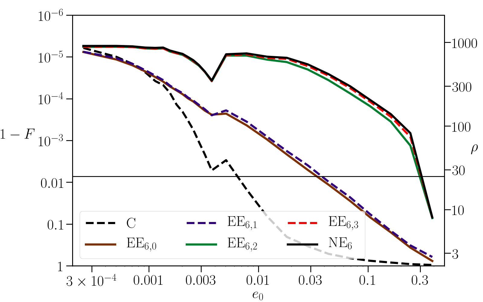
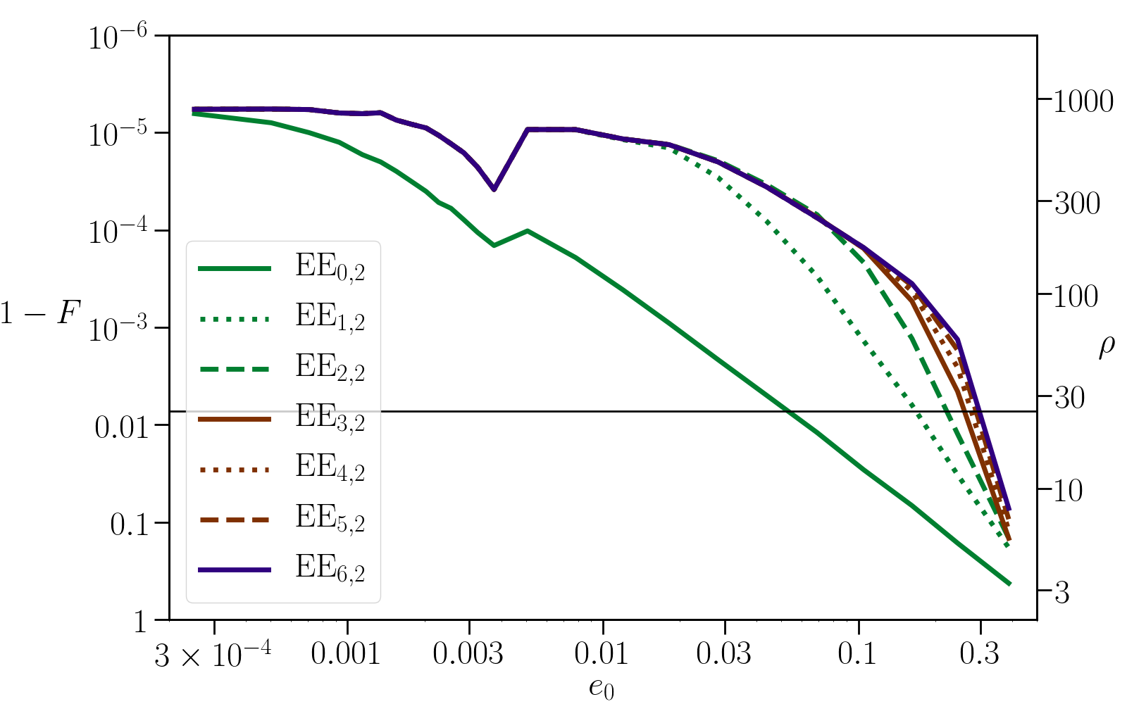
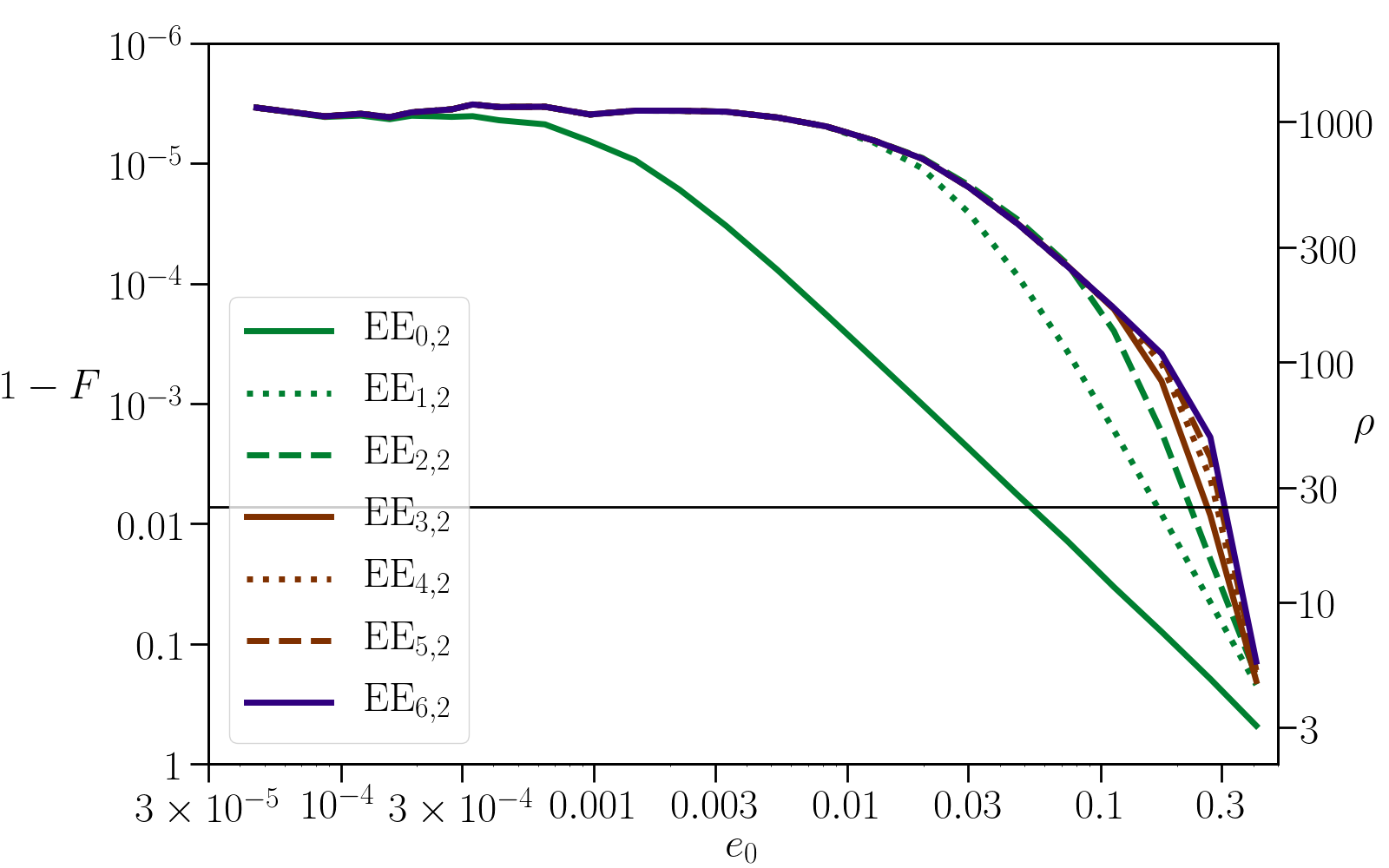
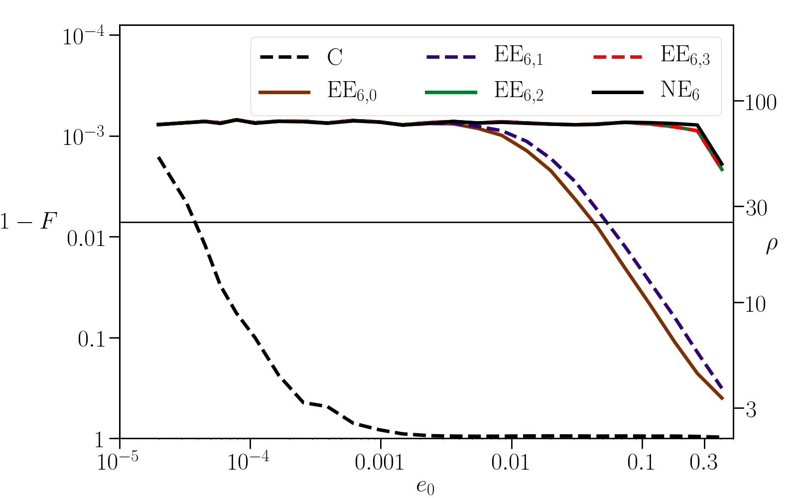
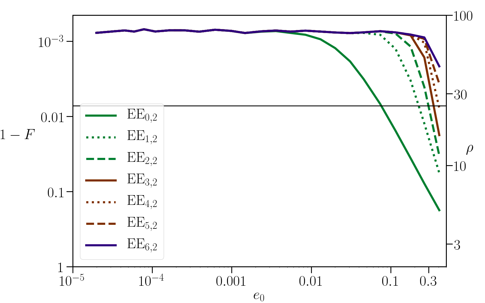
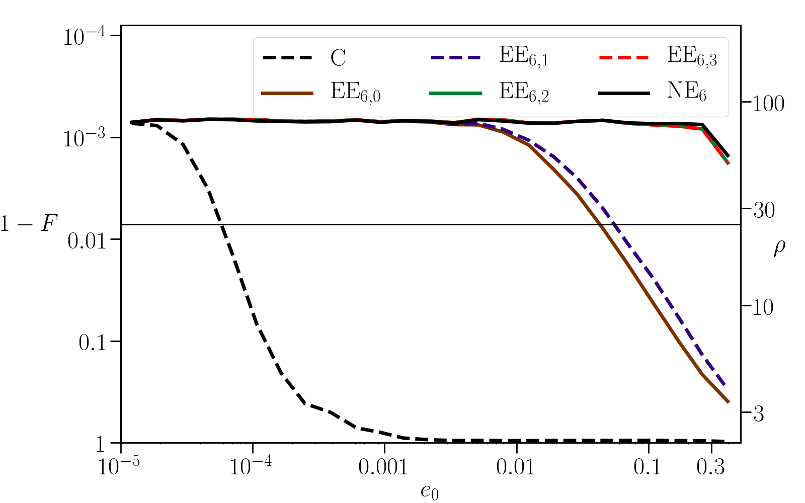
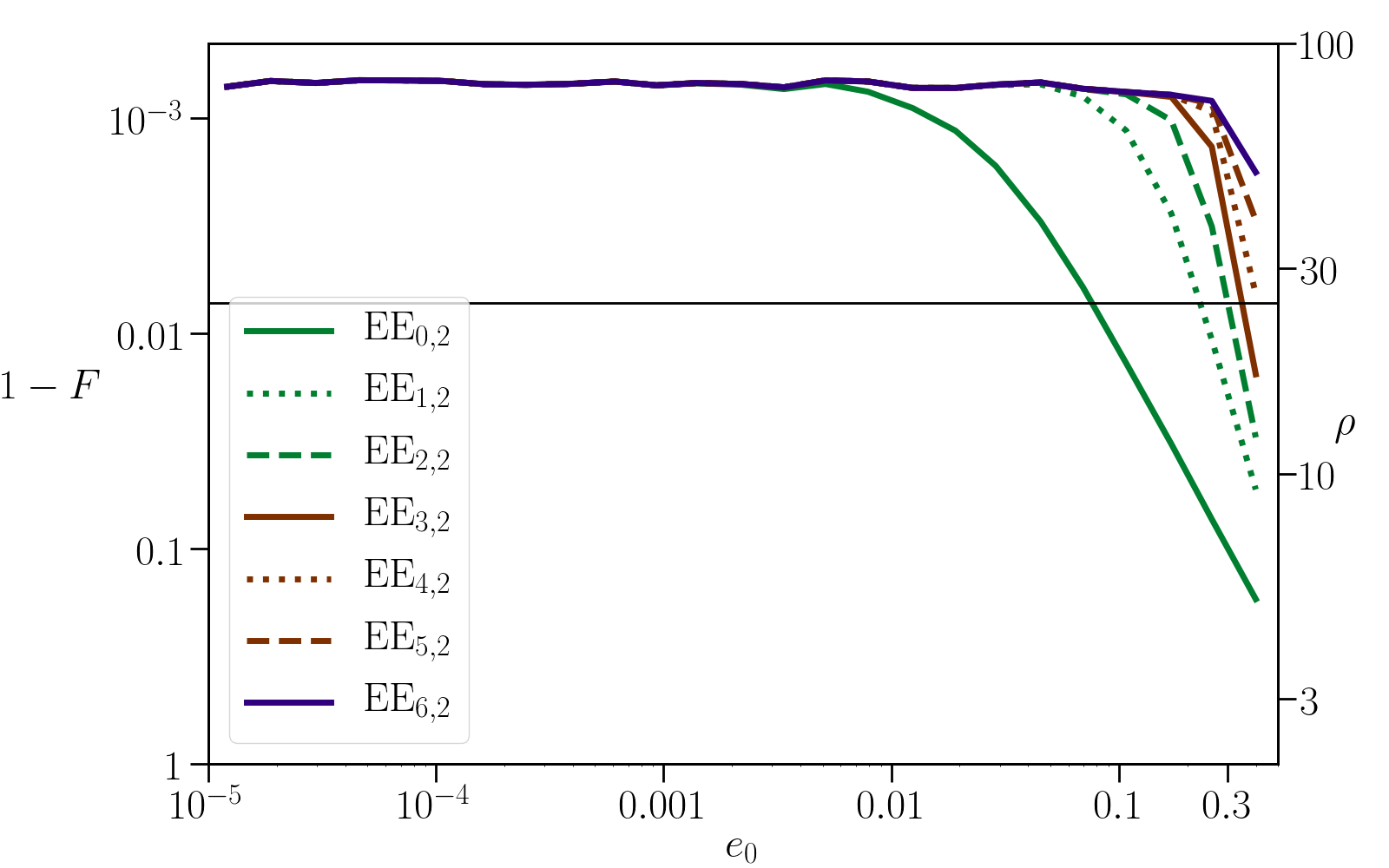
We present in Fig. 2 the results from late inspiral run (Ia), with starting eccentricity $10^{-5}<e_{0}<0.5$ and spin magnitudes $0<\chi_{i}<1$. In it, we compare the mean faithfulness as a function of the initial eccentricity for different waveforms. The top panel shows a comparison between the results for the circular waveform C, the nonexpanded eccentric waveform NE₆, and the expanded eccentric waveforms $EE_{6,P}$, $0\leq P\leq 3$, and the bottom panel shows a comparison between the expanded eccentric waveforms EE_M,2, $0\leq M\leq 6$. We can see in the top panel that the circular waveform stays above the fiducial faithfulness only for initial eccentricities of $e_{0}\lesssim 0.008$. Furthermore, the results for the expanded eccentric waveform become very close to the nonexpanded version starting at second order in $\delta\dot{\lambda}/\dot{\lambda}$, and leads to a faithfulness above the fiducial threshold for eccentricities below $e_{0}\lesssim 0.3$. On the bottom panel, we can see the effects of the expansion of the waveform amplitudes for small eccentricities. We can see that the largest starting eccentricity for which the median faithfulness stays above the threshold increases with increasing order in the expansion. Furthermore, we can see that below a certain starting eccentricity depending on the specific order, increasing the expansion order has no effect on the faithfulness, as the errors due to this approximation become subdominant.

Figure 3: Same as Fig. 2, for late inspiral run (IIa) with starting eccentricity $10^{-5}<e_{0}<0.5$ and spin magnitudes $0<\chi_{i}<0.1$.

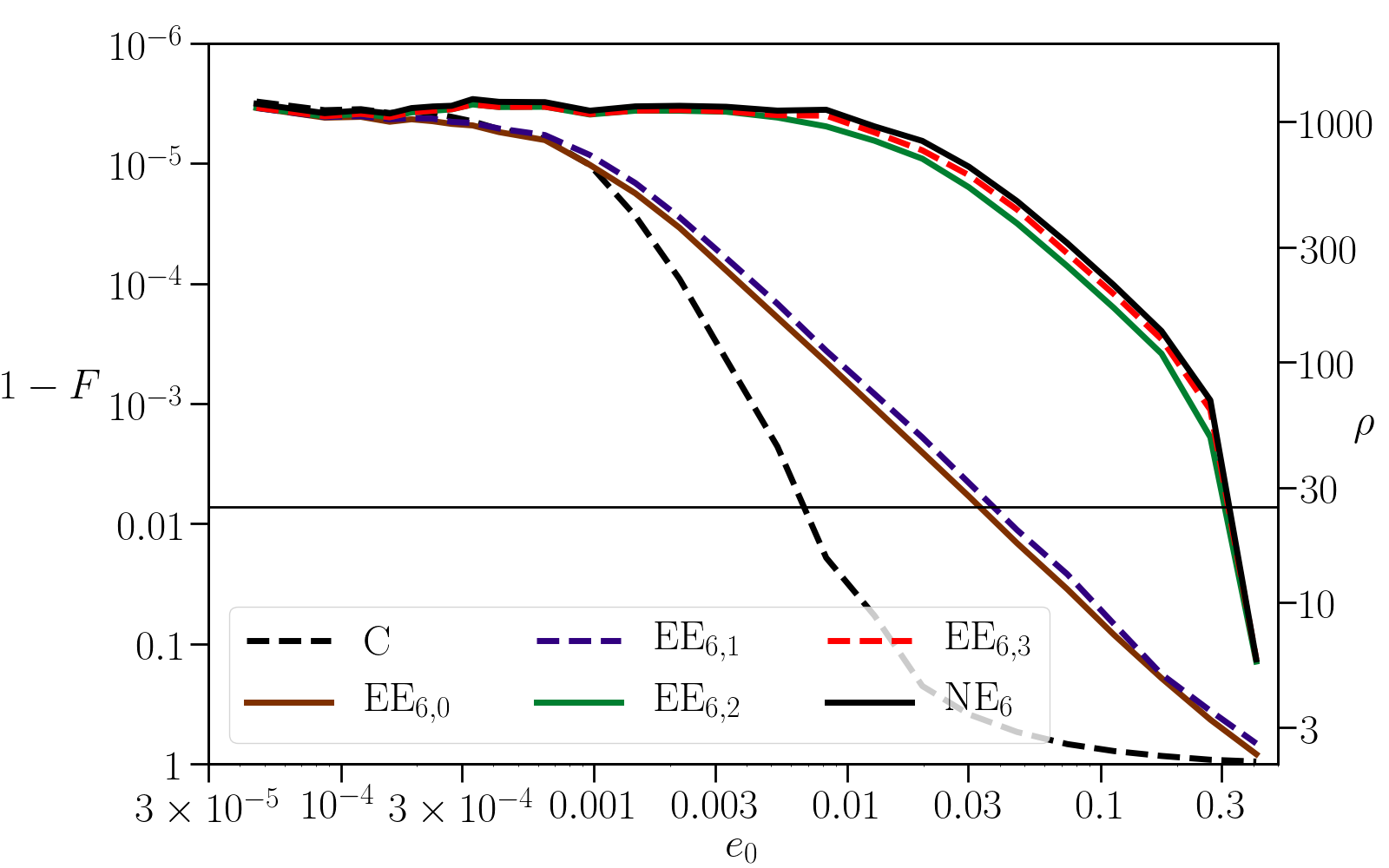
We present in Fig. 3 the results from late inspiral run (IIa), with starting eccentricity $10^{-5}<e_{0}<0.5$ and spin magnitudes $0<\chi_{i}<0.1$. These results are very similar to the results of run (Ia), but due to the reduced spin magnitudes the starting eccentricities reach smaller values. On the top panel, we can see that below a starting eccentricity of $e_{0}\lesssim 10^{-3}$, the loss of faithfulness using circular waveforms with respect to our eccentric models becomes negligible.

Figure 4: Same as Fig. 2, for late inspiral run (IIIa) with starting eccentricity $10^{-5}<e_{0}<0.5$ and spin magnitudes $\chi_{i}=1$.

We present in Fig. 4 the results from late inspiral run (IIIa), with starting eccentricity $10^{-5}<e_{0}<0.5$ and spin magnitudes $\chi_{i}=1$. The results are similar to the ones shown in Figs. 2 and 3, but the increased magnitudes of the spins slightly reduce the performance of the circular waveform. Comparing this figure to Figs. 2 and 3, we can conclude that the value of the spin magnitudes has little effect on the faithfulness, other than on the limiting residual eccentricity.

Figure 5: Results from late inspiral run (IVa) with starting eccentricity $e_{0}=e_{\text{min}}$ and spin magnitudes $0<\chi_{i}<1$. The systems simulated here correspond to highly spinning fully circularized binaries. The blue line corresponds to the circular waveform C, the red line to the lowest-order expanded eccentric waveform EE_0,0, and the green line to the highly accurate expanded eccentric waveform EE_6,2. The bottom axis shows the unfaithfulness $1-F$, and the top axis shows the corresponding threshold SNR $\rho$ above which we can expect mismodeling errors to exceed the accuracy in a measurement. The thin vertical line corresponds to a fiducial faithfulness of 0.993 or a corresponding SNR of 25. Note that due to the eccentricity being taken into account in the phasing, even the lowest-order eccentric waveform EE_0,0 performs better than the circular waveform C.

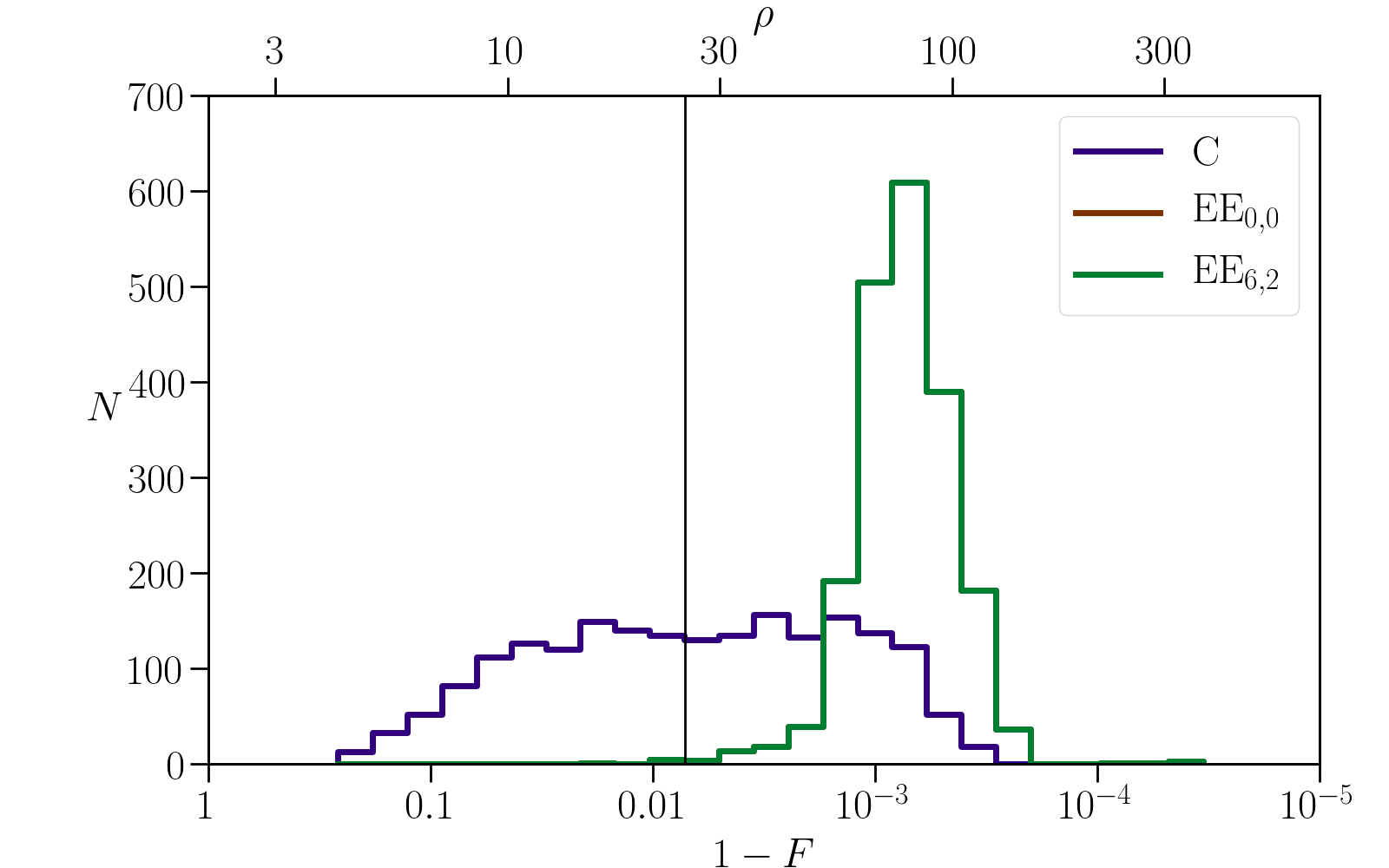
We present in Fig. 5 the results from late inspiral run (IVa), with starting eccentricity $e_{0}=e_{\text{min}}$ and spin magnitudes $0<\chi_{i}<1$. We can see here an effect due to the residual eccentricity. Indeed, the circular waveform performs poorly in some cases, even when the binaries are fully circularized. In our simulations, 7% of the faithfulness for the circular waveform was below the threshold line, while virtually no faithfulness were found below it for waveforms that used eccentric phasing, even with the lowest order amplitudes. While this does not represent a large proportion of binaries, this number will only increase when considering binaries with higher SNRs.

Figure 6: Same as Fig. 5, for late inspiral run (Va) with starting eccentricity $e_{0}=e_{\text{min}}$ and spin magnitudes $0<\chi_{i}<0.1$. The systems simulated here correspond to slowly spinning fully circularized binaries.

We present in Fig. 6 the results from late inspiral run (Va), with starting eccentricity $e_{0}=e_{\text{min}}$ and spin magnitudes $0<\chi_{i}<0.1$. Comparing with the results shown in Fig. 5, we can see that assuming lower spins prevents the circular waveforms from having faithfulness below the threshold line. Thus, eccentricity effects in the inspiral can be safely ignored when only the last part of it is visible. This further shows that the starting eccentricity is the most important factor to influencing the accuracy of our waveforms in the late inspiral.

Figure 7: Same as Fig. 5, for late inspiral run (VIa) with starting eccentricity $e_{0}=e_{\text{min}}$ and spin magnitudes $\chi_{i}=1$. The systems simulated here correspond to maximally spinning fully circularized binaries.

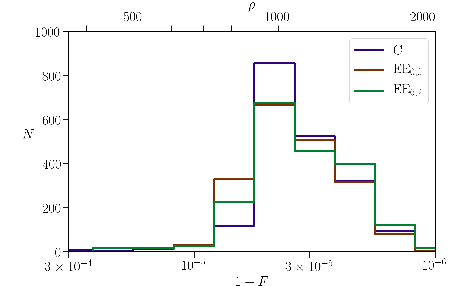
We present in Fig. 7 the results from late inspiral run (VIa), with starting eccentricity $e_{0}=e_{\text{min}}$ and spin magnitudes $\chi_{i}=1$. The results here are similar to the ones shown in Fig. 5, but more pronounced. The proportion of binaries for which the circular waveform has a faithfulness lying below the threshold line increases to 25 %, indicating that the inclusion of eccentricity effects might be important even for fully circularized binaries in the last stages of their inspiral when their spins are large.

III.2 Early inspiral systems

Figure 8: Same as Fig. 2, for early inspiral run (Ib) with starting eccentricity $10^{-5}<e_{0}<0.5$ and spin magnitudes $0<\chi_{i}<1$.

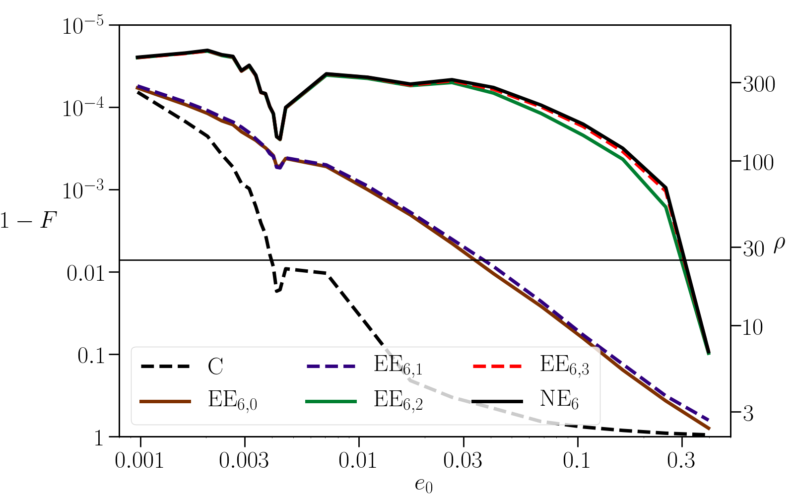
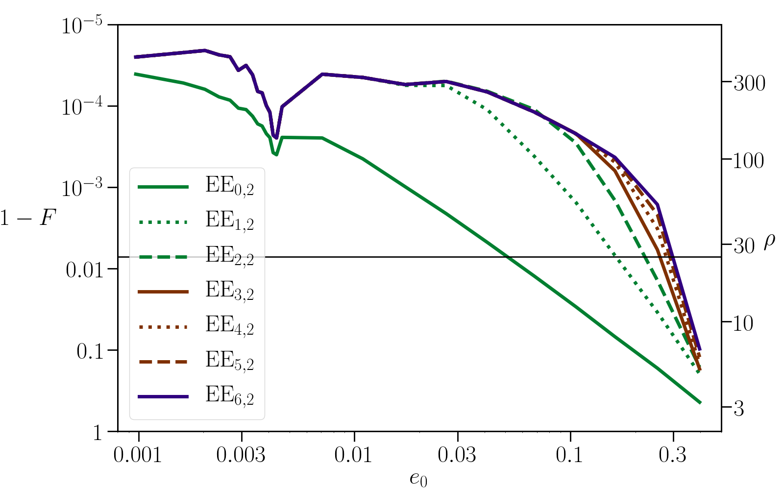
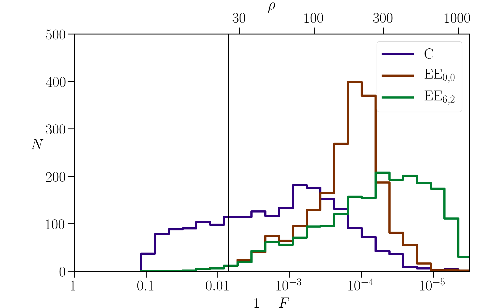
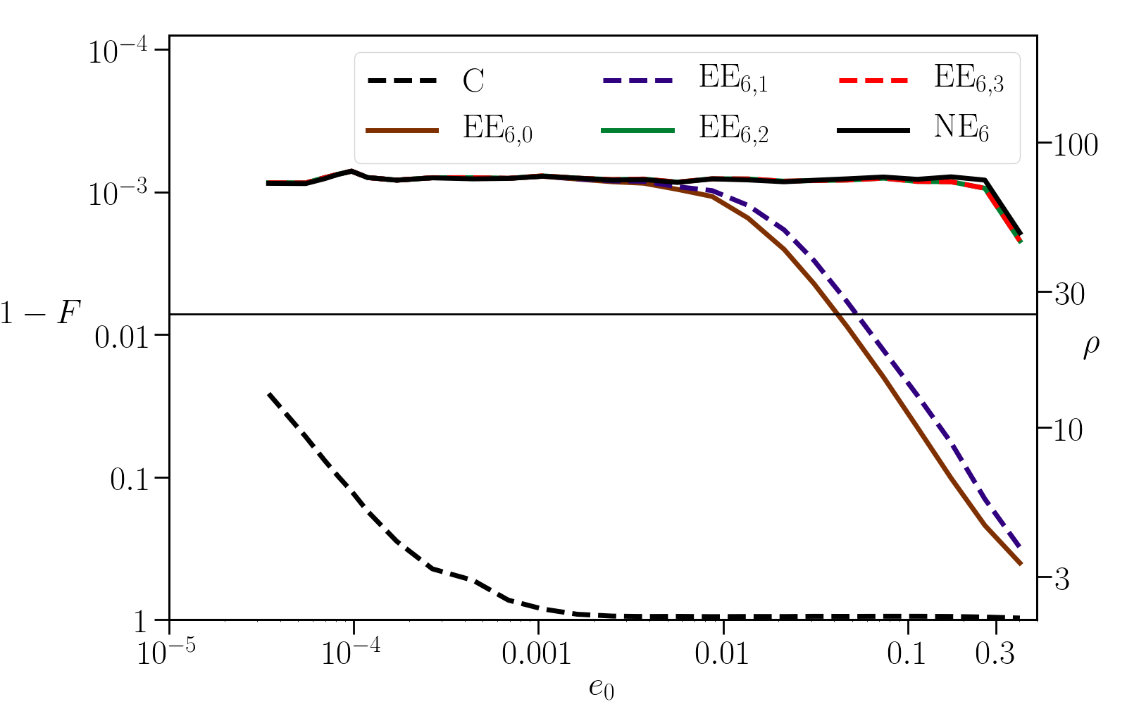
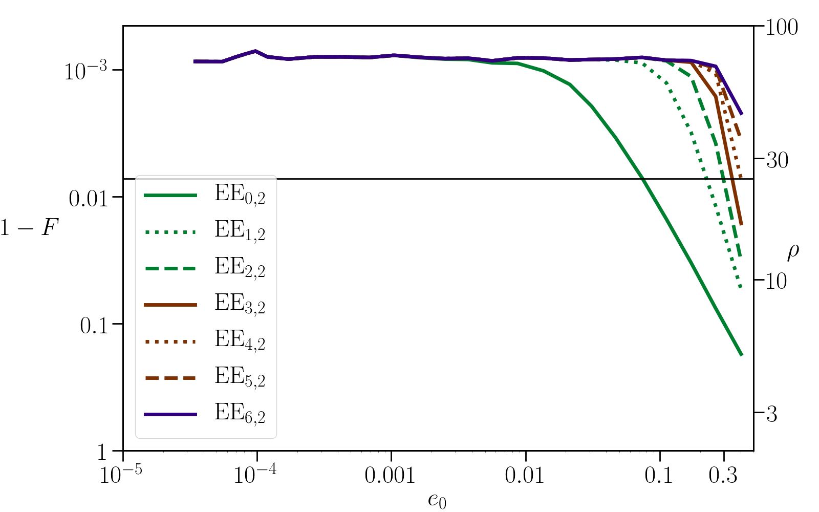
We present in Fig. 8 the results from early inspiral run (Ib), with starting eccentricity $10^{-5}<e_{0}<0.5$ and spin magnitudes $0<\chi_{i}<1$. We can see that, in this case, using circular waveforms will likely result in large biases even when the starting eccentricity is below $10^{-3}$. The large number of orbital cycles accumulated is such that the small difference in the frequency evolution induces very low faithfulness even for very low eccentricities. On the other hand, the eccentric waveforms perform better than in the late inspiral case. In the top panel, we can see that the low-order EE_6,0 waveform stays above the faithfulness threshold for $e_{0}\lesssim 0.05$, while the high-order one EE_6,2 is above the threshold for the whole parameter space that we investigated. In the bottom panel, we can see that the waveform with circular amplitudes EE_0,2 stays above the threshold for $e_{0}\lesssim 0.1$, while the waveforms EE_M,2, $M\geq 2$ do so for $e_{0}\lesssim 0.3$.

Figure 9: Same as Fig. 2, for early inspiral run (IIb) with starting eccentricity $10^{-5}<e_{0}<0.5$ and spin magnitudes $0<\chi_{i}<0.1$.

We present in Fig. 9 the results from early inspiral run (IIb), with starting eccentricity $10^{-5}<e_{0}<0.5$ and spin magnitudes $0<\chi_{i}<0.1$. We can see that, for initial eccentricities $e_{0}\gtrsim 10^{-4}$, circular waveforms yield a faithfulness below $F=0.9$. Thus, even if they are slowly spinning, the use of circular waveforms for parameter estimation for such binaries is likely to yield important biases. Using eccentric waveforms for early inspiral systems is therefore crucial in order to ensure accurate parameter recovery, even with initial eccentricities as low as $e_{0}\sim 10^{-4}$. In the bottom panel, similarly to run (Ib), we can see that the waveform with circular amplitudes EE_0,2 stays above the threshold for $e_{0}\lesssim 0.1$, while the waveforms EE_M,2, $M\geq 2$ do so for $e_{0}\lesssim 0.3$.

Figure 10: Same as Fig. 2, for early inspiral run (IIIb) with starting eccentricity $10^{-5}<e_{0}<0.5$ and spin magnitudes $\chi_{i}=1$.

We present in Fig. 10 the results from early inspiral run (IIIb), with starting eccentricity $10^{-5}<e_{0}<0.5$ and spin magnitudes $\chi_{i}=1$. While the results for the eccentric waveforms are similar to the ones shown in Figs. 8 and 9, the circular waveform never reached a median faithfulness above the threshold line above an initial eccentricity of $e_{0}=3\times 10^{-5}$. This indicates that highly spinning systems in the early inspiral will require the use of an eccentric model irrespective of their initial eccentricity.

Figure 11: Same as Fig. 5, for early inspiral run (IVb) with starting eccentricity $e_{0}=e_{\text{min}}$ and spin magnitudes $0<\chi_{i}<1$. The systems simulated here correspond to highly spinning fully circularized binaries.

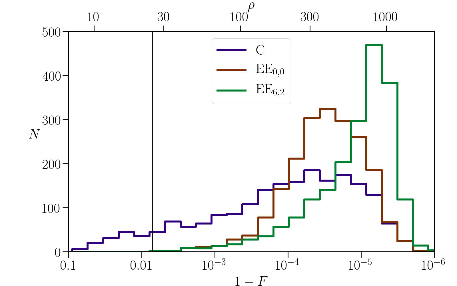
We present in Fig. 11 the results from early inspiral run (IVb), with starting eccentricity $e_{0}=e_{\text{min}}$ and spin magnitudes $0<\chi_{i}<1$. We can see that for these systems, including the eccentricity in the phasing is important, but the order used in other effects matters very little. Indeed, the faithfulness distributions for the two eccentric waveforms EE_0,0 and EE_6,2 are indistinguishable and have support almost exclusively above the faithfulness threshold, whereas the faithfulness distribution for the circular waveforms has 46 % support below the threshold.

Figure 12: Same as Fig. 5, for early inspiral run (Vb) with starting eccentricity $e_{0}=e_{\text{min}}$ and spin magnitudes $0<\chi_{i}<0.1$. The systems simulated here correspond to slowly spinning fully circularized binaries.

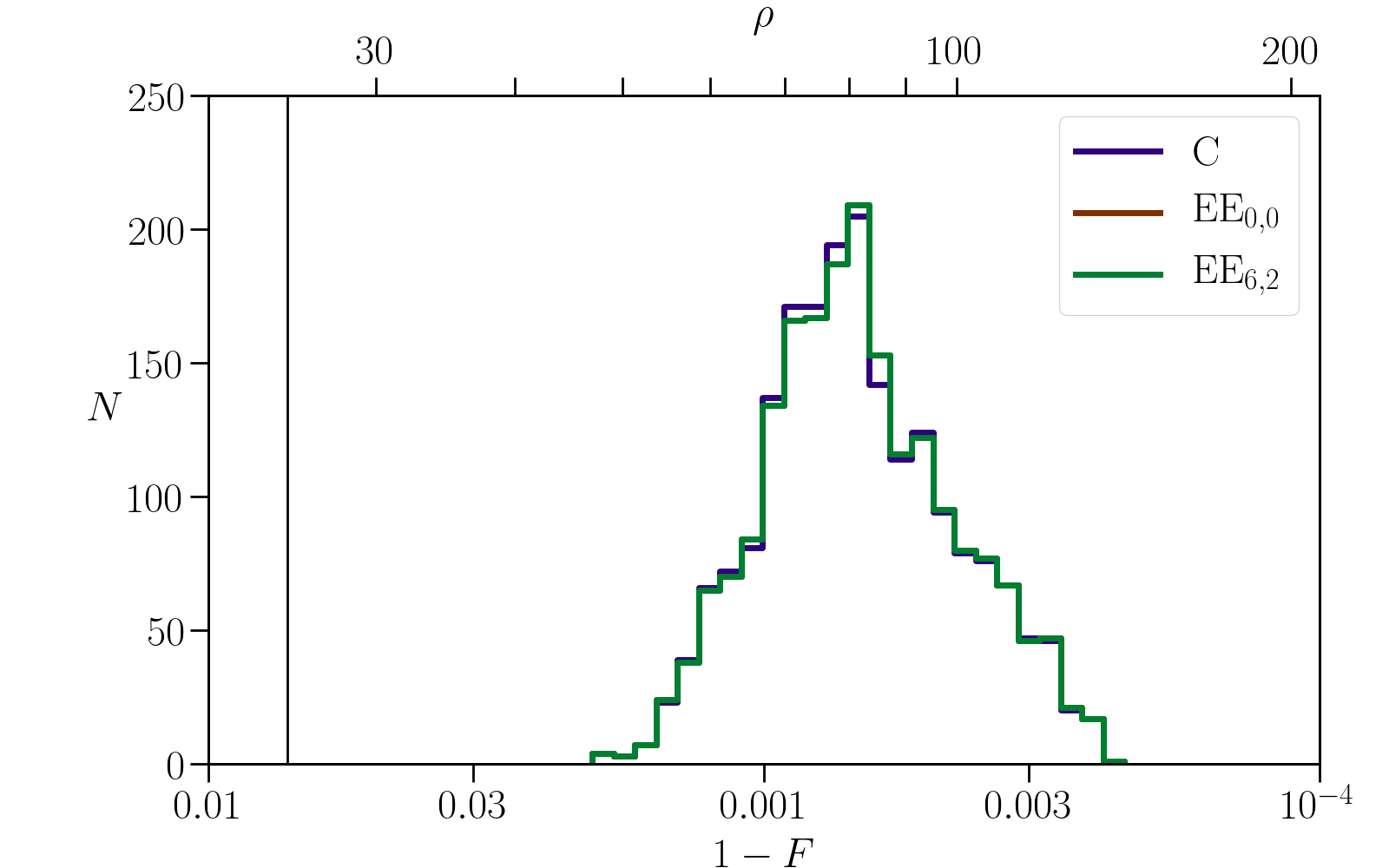
We present in Fig. 12 the results from early inspiral run (Vb), with starting eccentricity $e_{0}=e_{\text{min}}$ and spin magnitudes $0<\chi_{i}<0.1$. We can see that for these systems, circular waveforms have a faithfulness distribution almost identical to those of eccentric waveforms, indicating that when the spins are small and the binaries have fully circularized, the use of circular waveforms may be sufficient for unbiased parameter estimation.

Figure 13: Same as Fig. 5, for early inspiral run (VIb) with starting eccentricity $e_{0}=e_{\text{min}}$ and spin magnitudes $\chi_{i}=1$. The systems simulated here correspond to maximally spinning fully circularized binaries.

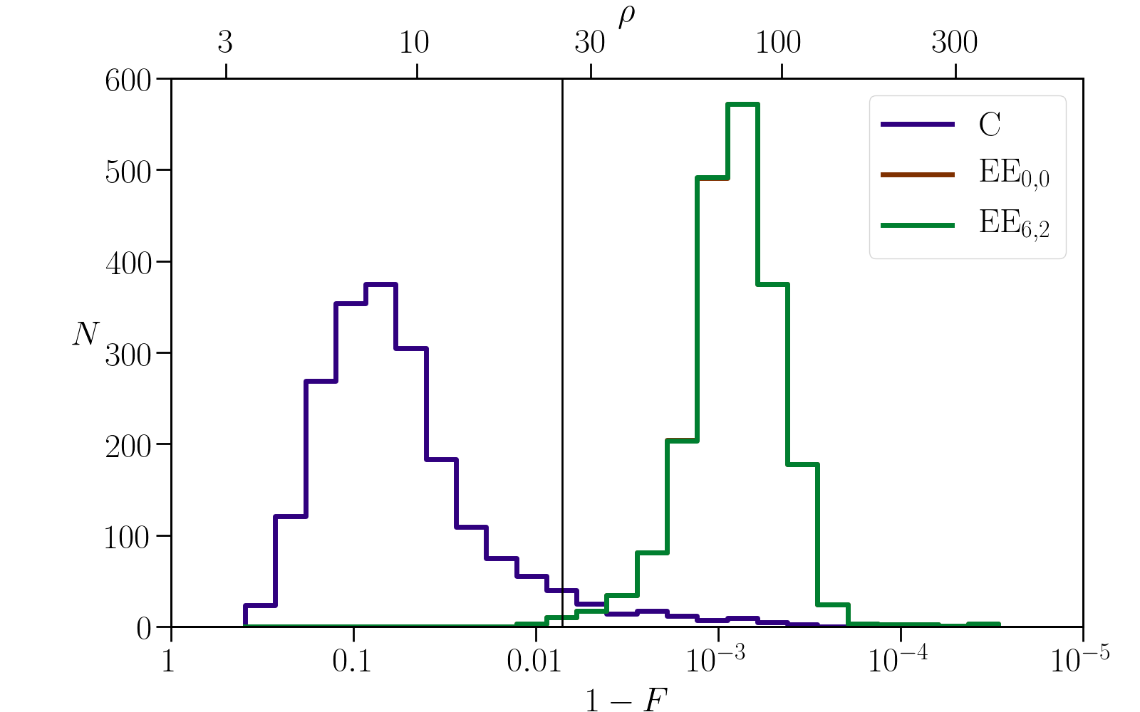
We present in Fig. 13 the results from early inspiral run (VIb), with starting eccentricity $e_{0}=e_{\text{min}}$ and spin magnitudes $\chi_{i}=1$. We observe in this figure that the faithfulness distribution for the circular waveforms has 94% support below the threshold line, indicating that for highly spinning binaries, the use of eccentric waveforms will be crucial for unbiased parameter estimation. However, the distributions for the two eccentric waveforms EE_0,0 and EE_6,2 are indistinguishable also in this case, indicating that the precision of the waveform amplitude is of little importance. Thus, eccentricity and spins will be important to include in the analysis of stellar-origin black hole binaries with LISA to account for the possibility of high spins, even if the binaries have fully circularized. However, using accurate amplitudes might be unnecessary for those sources.

Waveform	$e_{0}^{\text{max,l}}$		$e_{0}^{\text{max,e}}$
C	$0.0078$		$<7\times 10^{-5}$
EE0,0	$0.056$		$0.086$
EE6,0	$0.036$		$0.04$
EE0,2	$0.056$		$0.086$
EE2,2	$0.23$		$0.32$
EE4,2	$0.29$		$>0.4$
EE6,2	$0.32$		$>0.4$
NE6	$0.33$		$>0.4$

Table 1: For a few select waveforms, maximum initial eccentricity $e_{0}^{\text{max,l}}$ for which the median faithfulness in the late inspiral runs stays above the faithfulness threshold, and the same for the early inspiral runs $e_{0}^{\text{max,e}}$.

Comparing the different results, we find that the median faithfulness for each waveform is mainly influenced by the initial eccentricity, and the stage in the inspiral that they find themselves in. We summarize in Table 1 the initial eccentricity below which the median faithfulness falls above the threshold line for a few of the waveforms compared in our simulations. Interestingly, we find that waveform EE_0,0 performs slightly better than waveform EE_6,0. We find the same to be true by comparing EE_0,0 to any waveform EE_M,0 or EE_M,1 with $M>0$. We thus remark that in order for the inclusion of beyond-circular effects in the amplitudes to increase the accuracy of the waveform, one also needs to include periastron precession effects at least at second order.

IV Conclusion

We have constructed two families of Fourier domain waveforms for spin-precessing binaries on eccentric orbits. These include phasing at the third nonspinning post-Newtonian order, including leading-order spin-orbit and spin-spin interactions, as well as instantaneous amplitudes at second post-Newtonian order as small eccentricity expansions. In this work, we have used amplitudes up to $\mathcal{O}\left(e^{6}\right)$, but the extension to higher orders in the eccentricity would be trivial though lengthy. Through comparisons with a complete time domain waveform at consistent post-Newtonian order, we find that our new waveforms faithfully reproduce their Fourier transform for initial eccentricities up to $e_{0}\sim 0.3$ for systems in the late inspiral, and at least up to $e_{0}\sim 0.4$ for systems in the early inspiral such as stellar-origin black hole binaries as observed by LISA.

Comparing results, we find that using circular waveforms would likely lead to significant biases in parameter recovery, even for fully circularized binaries with a signal-to-noise ratio around 25, provided they are highly spinning. Indeed, a 2PN spin effect prevents the eccentricity of a binary system from vanishing completely unless the projections of the reduced spins in the orbital plane are exactly equal to each other. We find that the use of circular waveforms can cause biases if fully circularized systems with large spin magnitudes and random orientations are observed in the late inspiral, but not if the spin magnitudes are small. This situation is made worse if binary systems are observed in the early inspiral, and we expect large biases with circular waveforms irrespective of the initial eccentricity for highly spinning systems, even if they are fully circularized. However, if the spins are sufficiently small and the binaries have circularized below an eccentricity of $10^{-4}$ when the observations start, we expect the use of circular waveforms to be appropriate for parameter estimation. Overall, we expect circular waveforms to be safe to use for parameter estimation in the late inspiral if the initial eccentricity falls below $10^{-2}$ and in the early inspiral when it falls below $10^{-4}$, but we would recommend the use of eccentric phasing in the waveform to describe highly spinning systems, even if they have fully circularized.

Those waveforms provide a step towards the inclusion of the eccentricity in gravitational wave data analysis such as that performed by the LIGO/Virgo community. We argue from the simulations described in this paper that the inclusion of spins and eccentricity might be of importance for reducing potential biases in the parameter recovery of binaries, even when they are fully circularized. While circular templates might be appropriate to describe slowly spinning systems, it can be important to include in the modeling of highly spinning systems. It is worth noting that the faithfulness measurements described in this work are not suitable to estimate the loss of events due to mismodeling, or the measurability of binary parameters, including the initial eccentricity. We leave those questions open for future work.

Some assumptions made in this work, particularly the neglect of orbital timescale effects in the spin-orbit precession dynamics, have to be more closely investigated. Furthermore, the inclusion of the merger and ringdown signals in our waveforms is also very important work for the future, and will have to be taken into account in the construction of waveform templates to use in current and future detectors. The waveform that we have presented in this work, while useful to describe inspiral-dominated signals such as stellar-origin black hole binaries in LISA or neutron star binaries in the LIGO/Virgo network, is inspiral-only and therefore cannot be used alone in the characterization of merger-dominated signals such as black hole binaries as observed by the LIGO/Virgo network.

Appendix A Quadrupole-monopole effects

The 2PN part of the quasi-Keplerian parametrization found in Klein and Jetzer (2010) is based upon the reduced Lagrangian

$$\frac{\mathcal{L}}{\nu} =\frac{\dot{\bm{r}}^{2}}{2}+\frac{1}{r}+\frac{1}{r^{3}}\bm{s}_{1}\cdot\bm{s}_{2}-\frac{3}{r^{3}}\left(\bm{\hat{r}}\cdot\bm{s}_{1}\right)\left(\bm{\hat{r}}\cdot\bm{s}_{2}\right)\,,$$ (53)

where the reduced spins $\bm{s}_{i}=\bm{S}_{i}/m_{i}$. The quadrupole-monopole part of the reduced Lagrangian is Poisson (1998); Keresztes et al. (2005)

$$\frac{\mathcal{L}_{\text{QM}}}{\nu} =\frac{1}{2r^{3}}\sum_{i=1}^{2}q_{i}\left[\bm{s}_{i}^{2}-3\left(\bm{\hat{r}}\cdot\bm{s}_{i}\right)^{2}\right]\,,$$ (54)

where the quadrupole parameter $q_{i}$ is defined in such a way that $q_{i}=1$ for black holes. The total Lagrangian can then be written as

$$\frac{\mathcal{L}}{\nu} =\frac{\dot{\bm{r}}^{2}}{2}+\frac{1}{r}+\frac{1}{2r^{3}}\bm{s}^{2}-\frac{3}{2r^{3}}\left(\bm{\hat{r}}\cdot\bm{s}\right)^{2}+\frac{1}{2r^{3}}\sum_{i=1}^{2}\left(q_{i}-1\right)\left[\bm{s}_{i}^{2}-3\left(\bm{\hat{r}}\cdot\bm{s}_{i}\right)^{2}\right]\,,$$ (55)

where $\bm{s}=\bm{s}_{1}+\bm{s}_{2}$.

Thus, a quasi-Keplerian description of the orbit including quadrupole-monopole terms can be found by adding the 2PN terms of Klein and Jetzer (2010), using the substitutions $(\bm{s}_{1}\to\bm{s}/\sqrt{2},\bm{s}_{2}\to\bm{s}/\sqrt{2})$, $(\bm{s}_{1}\to\bm{s}_{1}\sqrt{(q_{1}-1)/2},\bm{s}_{2}\to\bm{s}_{1}\sqrt{(q_{1}-1)/2})$, and $(\bm{s}_{1}\to\bm{s}_{2}\sqrt{(q_{2}-1)/2},\bm{s}_{2}\to\bm{s}_{2}\sqrt{(q_{2}-1)/2})$. It reads

$$r =a(1-e_{r}\cos u)+f_{r}(v)\,,$$ (56a)

$$\phi =(1+k)v+f_{\phi,1}(v)+f_{\phi,2}(v)\,,$$ (56b)

$$\tan\frac{v}{2} =\sqrt{\frac{1+e_{\phi}}{1-e_{\phi}}}\tan\frac{u}{2}\,,$$ (56c)

$$l =u-e\sin u\,,$$ (56d)

$$\dot{l} =n\,,$$ (56e)

with

$$a =\frac{1}{\left(1-e^{2}\right)y^{2}}\left[1+\frac{1}{2}\left(1+e^{2}\right)\gamma_{1}y^{4}\right]\,,$$ (57a)

$$e_{r}^{2} =e^{2}\left[1+\left(1-e^{2}\right)\gamma_{1}y^{4}\right]\,,$$ (57b)

$$k =\frac{3}{2}\gamma_{1}y^{4}\,,$$ (57c)

$$e_{\phi}^{2} =e^{2}\left[1+2\left(1-e^{2}\right)\gamma_{1}y^{4}\right]\,,$$ (57d)

$$n =\left(1-e^{2}\right)^{3/2}y^{3}\left(1-\frac{3}{2}\gamma_{1}y^{4}\right)\,,$$ (57e)

$$\gamma_{1} =\frac{1}{2}\left\{3\left(\bm{\hat{L}}\cdot\bm{s}\right)^{2}-\bm{s}^{2}+\sum_{i=1}^{2}\left(q_{i}-1\right)\left[3\left(\bm{\hat{L}}\cdot\bm{s}_{i}\right)^{2}-\bm{s}_{i}^{2}\right]\right\}\,,$$ (57f)

$$f_{r}(v) =-\frac{y^{2}}{4}\left[\left|\bm{\hat{L}}\times\bm{s}\right|^{2}\cos(2v-2\psi)+\sum_{i=1}^{2}\left(q_{i}-1\right)\left|\bm{\hat{L}}\times\bm{s}_{i}\right|^{2}\cos(2v-2\psi_{i})\right]\,,$$ (57g)

$$f_{\phi,1}(v) =-\frac{y^{4}e}{2}\left[\left|\bm{\hat{L}}\times\bm{s}\right|^{2}\sin(v-2\psi)+\sum_{i=1}^{2}\left(q_{i}-1\right)\left|\bm{\hat{L}}\times\bm{s}_{i}\right|^{2}\sin(v-2\psi_{i})\right]\,,$$ (57h)

$$f_{\phi,2}(v) =-\frac{y^{4}}{8}\left[\left|\bm{\hat{L}}\times\bm{s}\right|^{2}\sin(2v-2\psi)+\sum_{i=1}^{2}\left(q_{i}-1\right)\left|\bm{\hat{L}}\times\bm{s}_{i}\right|^{2}\sin(2v-2\psi_{i})\right]\,,$$ (57i)

where $\psi$ is the angle subtended by the total reduced spin $\bm{s}$ and the periastron line, $\psi_{i}$ is the angle subtended by the individual reduced spin $\bm{s}_{i}$ and the periastron line (see Fig. 1), and the periastron line is defined by the equation $v=u=l=2p\pi$, $p\in\mathbb{Z}$. We can then use this representation of the orbit together with the orbit averaged evolution equations for the energy and orbital angular momentum computed in Gergely and Keresztes (2003) to find

$$M\frac{dy}{dt}= \;\nu\left(1-e^{2}\right)^{3/2}\bigg{\{}\left(\frac{32}{5}+\frac{28}{5}e^{2}\right)y^{9}+\sigma\bigg{[}-\frac{84}{5}-\frac{228}{5}e^{2}-\frac{33}{5}e^{4},\frac{242}{5}+\frac{654}{5}e^{2}+\frac{381}{20}e^{4},-\frac{447}{10}e^{2}-\frac{93}{10}e^{4},$$

$$\frac{88}{5}-16q+\left(48-\frac{216}{5}q\right)e^{2}+\left(\frac{69}{10}-\frac{63}{10}q\right)e^{4},-\frac{244}{5}+48q+\left(-132+\frac{648}{5}q\right)e^{2}+\left(-\frac{96}{5}+\frac{189}{10}q\right)e^{4},$$

$$\left(1-q\right)\left(\frac{447}{10}e^{2}+\frac{93}{10}e^{4}\right)\bigg{]}y^{13}\bigg{\}}\,,$$ (58a)

$$M\frac{de^{2}}{dt}= \;-\nu\left(1-e^{2}\right)^{3/2}\bigg{\{}\left(\frac{608}{15}e^{2}+\frac{242}{15}e^{4}\right)y^{8}+\sigma\bigg{[}\frac{2}{3}-\frac{1961}{15}e^{2}-\frac{2527}{12}e^{4}-\frac{157}{8}e^{6},-\frac{2}{3}+\frac{5623}{15}e^{2}+\frac{2393}{4}e^{4}$$

$$+\frac{447}{8}e^{6},-\frac{5527}{30}e^{2}-\frac{10117}{30}e^{4}-\frac{5507}{160}e^{6},-\frac{4}{3}+\left(\frac{682}{5}-\frac{1876}{15}q\right)e^{2}+\left(\frac{1337}{6}-\frac{595}{3}q\right)e^{4}+\left(\frac{83}{4}-\frac{37}{2}q\right)e^{6},$$

$$\frac{4}{3}+\left(-\frac{5618}{15}+\frac{1876}{5}q\right)e^{2}+\left(-\frac{1203}{2}+595q\right)e^{4}+\left(-\frac{225}{4}+\frac{111}{4}q\right)e^{6},$$

$$\left(\frac{2764}{15}-\frac{921}{5}q\right)e^{2}+\left(\frac{1687}{5}-\frac{5056}{15}q\right)e^{4}+\left(\frac{551}{16}-\frac{172}{5}q\right)e^{6}\bigg{]}y^{12}\bigg{\}}\,,$$ (58b)

where

$$\sigma(a,b,c,a_{1}+a_{2}q,b_{1}+b_{2}q,c_{1}+c_{2}q)= \;a\bm{s}^{2}+b\left(\bm{\hat{L}}\cdot\bm{s}\right)^{2}+c\left|\bm{\hat{L}}\times\bm{s}\right|^{2}\cos 2\psi$$

$$+\sum_{i=1}^{2}\left[\left(a_{1}+a_{2}q_{i}\right)\bm{s}_{i}^{2}+\left(b_{1}+b_{2}q_{i}\right)\left(\bm{\hat{L}}\cdot\bm{s}_{i}\right)^{2}+\left(c_{1}+c_{2}q_{i}\right)\left|\bm{\hat{L}}\times\bm{s}_{i}\right|^{2}\cos 2\psi_{i}\right]\,.$$ (59)

We thus find the residual eccentricity found in Klein and Jetzer (2010) unchanged by quadrupole-monopole effects.

Appendix B Quasi-Keplerian parametrization

A full quasi-Keplerian parametrization of the orbit at 2PN order in harmonic coordinates is Memmesheimer et al. (2004); Klein and Jetzer (2010)

$$r =a(1-e_{r}\cos u)+f_{r}(v)\,,$$ (60a)

$$\phi =(1+k)v+f_{\phi}(v)\,,$$ (60b)

$$\tan\frac{v}{2} =\sqrt{\frac{1+e_{\phi}}{1-e_{\phi}}}\tan\frac{u}{2}\,,$$ (60c)

$$l =u-e\sin u+f_{t}(u,v)\,,$$ (60d)

$$\dot{l} =n\,,$$ (60e)

with

$$a= \;\frac{1}{\left(1-e^{2}\right)y^{2}}\bigg{\{}1+\left[-1+\frac{\nu}{3}+\left(3-\frac{\nu}{3}\right)e^{2}\right]y^{2}+\beta\left(\frac{2}{3}+2e^{2},1+e^{2}\right)y^{3}+\bigg{[}5+\frac{11}{4}\nu+\frac{\nu^{2}}{9}$$

$$+\bigg{(}\frac{21}{2}-\frac{73}{6}\nu-\frac{2}{9}\nu^{2}\bigg{)}e^{2}+\left(1+\frac{5}{12}\nu+\frac{\nu^{2}}{9}\right)e^{4}+\left(1-e^{2}\right)^{3/2}\left(-5+2\nu\right)+\frac{\gamma_{1}}{2}\left(1+e^{2}\right)\bigg{]}y^{4}\,,$$ (61a)

$$e_{r}^{2}= \;e^{2}\bigg{\{}1+\left(1-e^{2}\right)\bigg{\{}\left(8-3\nu\right)y^{2}+\beta\left(4,2\right)y^{3}+\bigg{[}32-\frac{467}{12}\nu+4\nu^{2}+\left(-40+\frac{371}{12}\nu-4\nu^{2}\right)e^{2}$$

$$+\sqrt{1-e^{2}}\left(15-6\nu\right)+\gamma_{1}\bigg{]}y^{4}\bigg{\}}\bigg{\}}\,,$$ (61b)

$$k= \;3y^{2}+\beta\left(4,3\right)y^{3}+\left[\frac{27}{2}-7\nu+\left(\frac{51}{4}-\frac{13}{2}\nu\right)e^{2}+\frac{3}{2}\gamma_{1}\right]y^{4}\,,$$ (61c)

$$e_{\phi}^{2}= \;e^{2}\bigg{\{}1+\left(1-e^{2}\right)\bigg{\{}\left(8-2\nu\right)y^{2}+\beta\left(4,4\right)y^{3}+\bigg{[}42-\frac{113}{12}\nu+\frac{11}{12}\nu^{2}+\left(-40+\frac{1043}{48}\nu-\frac{89}{48}\nu^{2}\right)e^{2}$$

$$+\sqrt{1-e^{2}}\left(15-6\nu\right)+2\gamma_{1}\bigg{]}y^{4}\bigg{\}}\bigg{\}}\,,$$ (61d)

$$n= \;\left(1-e^{2}\right)^{3/2}y^{3}\bigg{\{}1-3y^{2}-\beta\left(4,3\right)y^{3}+\left[-\frac{9}{2}+7\nu+\left(-\frac{51}{4}+\frac{13}{2}\nu\right)e^{2}-\frac{3}{2}\gamma_{1}\right]y^{4}\bigg{\}}\,,$$ (61e)

where

$$\beta(a,b) =-\left[\left(a\mu_{1}+b\mu_{2}\right)\bm{s}_{1}+\left(b\mu_{1}+a\mu_{2}\right)\bm{s}_{2}\right]\cdot\bm{\hat{L}}\,,$$ (62a)

$$\gamma_{1} =\frac{1}{2}\left\{3\left(\bm{\hat{L}}\cdot\bm{s}\right)^{2}-\bm{s}^{2}+\sum_{i=1}^{2}\left(q_{i}-1\right)\left[3\left(\bm{\hat{L}}\cdot\bm{s}_{i}\right)^{2}-\bm{s}_{i}^{2}\right]\right\}\,.$$ (62b)

The functions $f_{r}$, $f_{\phi}$, $f_{t}$, and $f_{n}$ are given by

$$f_{r}(v) =\sum_{i=0}^{2}b_{r,i}\cos(2v-2\psi_{i})\,,$$ (63a)

$$f_{\phi}(v) =\sum_{k=2}^{3}a_{\phi,k}\sin(kv)+\sum_{k=1}^{2}\sum_{i=0}^{2}b_{\phi,k,i}\sin(kv-2\psi_{i})\,,$$ (63b)

$$f_{t}(u,v) =g_{t}(u-v)+a_{t}\sin(v)\,,$$ (63c)

with

$$b_{r,i} =-\frac{y^{2}}{4}F_{i}\left|\bm{\hat{L}}\times\bm{s}_{i}\right|^{2}\,,$$ (64a)

$$a_{\phi,2} =e^{2}\left(\frac{\nu}{8}-\frac{3}{8}\nu^{2}\right)y^{4}\,,$$ (64b)

$$a_{\phi,3} =-e^{3}\frac{3}{32}\nu^{2}y^{4}\,,$$ (64c)

$$b_{\phi,1,i} =-\frac{e}{2}F_{i}\left|\bm{\hat{L}}\times\bm{s}_{i}\right|^{2}y^{4}\,,$$ (64d)

$$b_{\phi,2,i} =-\frac{1}{8}F_{i}\left|\bm{\hat{L}}\times\bm{s}_{i}\right|^{2}y^{4}\,,$$ (64e)

$$g_{t} =\left(1-e^{2}\right)^{3/2}\left(\frac{15}{2}-3\nu\right)y^{4}\,,$$ (64f)

$$a_{t} =e\left(1-e^{2}\right)^{3/2}\left(-\frac{\nu}{2}-\frac{\nu^{2}}{8}\right)y^{4}\,,$$ (64g)

where we defined, for convenience, $\bm{s}_{0}=\bm{s}$, $\psi_{0}=\psi$, $F_{0}=1$, $F_{1}=q_{1}-1$, and $F_{2}=q_{2}-1$.

Appendix C Evolution equations

The evolution equations of $y$ and $e$ are given at 3PN order by  Arun et al. (2008a, b, 2009); Klein and Jetzer (2010)

$$M\frac{dy}{dt} =\left(1-e^{2}\right)^{3/2}\nu y^{9}\left(a_{0}+\sum_{n=2}^{6}a_{n}y^{n}\right)\,,$$ (65a)

$$M\frac{de^{2}}{dt} =-\left(1-e^{2}\right)^{3/2}\nu y^{8}\left(b_{0}+\sum_{n=2}^{6}b_{n}y^{n}\right)\,,$$ (65b)

where

$$a_{0}= \;\frac{32}{5}+\frac{28}{5}e^{2}\,,$$ (66a)

$$a_{2}= \;-\frac{1486}{105}-\frac{88}{5}\nu+\left(\frac{12296}{105}-\frac{5258}{45}\nu\right)e^{2}+\left(\frac{3007}{84}-\frac{244}{9}\nu\right)e^{4}\,,$$ (66b)

$$a_{3}= \;\frac{128\pi}{5}\phi_{y}+\beta\left(\frac{904}{15}+\frac{2224}{15}e^{2}+\frac{99}{5}e^{4},40+\frac{1916}{15}e^{2}+\frac{314}{15}e^{4}\right)\,,$$ (66c)

$$a_{4}= \;\frac{34103}{2835}+\frac{13661}{315}\nu+\frac{944}{45}\nu^{2}+\left(-\frac{256723}{945}-\frac{173587}{315}\nu+\frac{147443}{270}\nu^{2}\right)e^{2}+\left(\frac{2095517}{7560}-\frac{589507}{504}\nu+\frac{34679}{45}\nu^{2}\right)e^{4}$$

$$+\left(\frac{53881}{2520}-\frac{7357}{90}\nu+\frac{9392}{135}\nu^{2}\right)e^{6}+\frac{e^{2}}{1-e^{2}}\left(\frac{85}{6}+\frac{1445}{6}\nu\right)+\frac{1-\sqrt{1-e^{2}}}{\sqrt{1-e^{2}}}\bigg{[}16-\frac{32}{5}\nu+\left(266-\frac{532}{5}\nu\right)e^{2}$$

$$+\left(-\frac{859}{2}+\frac{859}{5}\nu\right)e^{4}+\left(-65+26\nu\right)e^{6}\bigg{]}+\sigma\bigg{[}-\frac{84}{5}-\frac{228}{5}e^{2}-\frac{33}{5}e^{4},\frac{242}{5}+\frac{654}{5}e^{2}+\frac{381}{20}e^{4},-\frac{447}{10}e^{2}-\frac{93}{10}e^{4},$$

$$\frac{88}{5}-16q+\left(48-\frac{216}{5}q\right)e^{2}+\left(\frac{69}{10}-\frac{63}{10}q\right)e^{4},-\frac{244}{5}+48q+\left(-132+\frac{648}{5}q\right)e^{2}+\left(-\frac{96}{5}+\frac{189}{10}q\right)e^{4},$$

$$\left(1-q\right)\left(\frac{447}{10}e^{2}+\frac{93}{10}e^{4}\right)\bigg{]}\,,$$ (66d)

$$a_{5}= \;\pi\left(-\frac{4159}{105}\psi_{y}-\frac{756}{5}\nu\zeta_{y}\right)\,,$$ (66e)

$$a_{6}= \;\frac{16447322263}{21829500}-\frac{54784}{525}\gamma_{E}+\frac{512}{15}\pi^{2}+\left(-\frac{56198689}{34020}+\frac{902}{15}\pi^{2}\right)\nu+\frac{541}{140}\nu^{2}-\frac{1121}{81}\nu^{3}+\bigg{[}\frac{247611308999}{87318000}$$

$$-\frac{392048}{525}\gamma_{E}+\frac{3664}{15}\pi^{2}+\left(-\frac{2828420479}{680400}+\frac{477}{4}\pi^{2}\right)\nu+\frac{1070903}{315}\nu^{2}-\frac{392945}{324}\nu^{3}\bigg{]}e^{2}+\bigg{[}-\frac{236637777001}{58212000}$$

$$-\frac{93304}{175}\gamma_{E}+\frac{872}{5}\pi^{2}+\left(\frac{2963572847}{453600}-\frac{53131}{960}\pi^{2}\right)\nu+\frac{44123941}{6048}\nu^{2}-\frac{2198212}{405}\nu^{3}\bigg{]}e^{4}+\bigg{[}-\frac{28913792717}{6468000}$$

$$-\frac{4922}{175}\gamma_{E}+\frac{46}{5}\pi^{2}+\left(\frac{107275139}{30240}-\frac{369}{80}\pi^{2}\right)\nu+\frac{5155951}{1512}\nu^{2}-\frac{44338}{15}\nu^{3}\bigg{]}e^{6}+\bigg{(}-\frac{243511057}{887040}+\frac{4179523}{15120}\nu$$

$$+\frac{83701}{3780}\nu^{2}-\frac{1876}{15}\nu^{3}\bigg{)}e^{8}+\frac{e^{2}}{1-e^{2}}\left[\frac{91284763}{378000}+\left(\frac{19505077}{5040}-\frac{595}{8}\pi^{2}\right)\nu-\frac{48569}{12}\nu^{2}-\frac{730168}{23625\left(1+\sqrt{1-e^{2}}\right)}\right]$$

$$+\frac{1-\sqrt{1-e^{2}}}{\sqrt{1-e^{2}}}\bigg{\{}-\frac{1425319}{3375}+\left(\frac{9874}{315}-\frac{41}{30}\pi^{2}\right)\nu+\frac{632}{15}\nu^{2}+\bigg{[}\frac{2385427}{1050}+\left(-\frac{274234}{45}+\frac{4223}{240}\pi^{2}\right)\nu+\frac{70946}{45}\nu^{2}\bigg{]}e^{2}$$

$$+\bigg{[}\frac{8364697}{4200}+\bigg{(}\frac{1900517}{630}-\frac{32267}{960}\pi^{2}\bigg{)}\nu-\frac{47443}{90}\nu^{2}\bigg{]}e^{4}+\bigg{[}-\frac{167385119}{25200}+\left(\frac{4272491}{504}-\frac{123}{160}\pi^{2}\right)\nu-\frac{43607}{18}\nu^{2}\bigg{]}e^{6}$$

$$+\bigg{(}-\frac{65279}{168}+\frac{510361}{1260}\nu-\frac{5623}{45}\nu^{2}\bigg{)}e^{8}\bigg{\}}+\frac{1284}{175}\kappa_{y}$$

$$+\left(\frac{54784}{525}+\frac{392048}{525}e^{2}+\frac{93304}{175}e^{4}+\frac{4922}{175}e^{6}\right)\log\left[\frac{1+\sqrt{1-e^{2}}}{8y\left(1-e^{2}\right)^{3/2}}\right]\,,$$ (66f)

$$b_{0}= \;\frac{608}{15}e^{2}+\frac{242}{15}e^{4}\,,$$ (66g)

$$b_{2}= \;\left(-\frac{1878}{35}-\frac{8168}{45}\nu\right)e^{2}+\left(\frac{59834}{105}-\frac{7753}{15}\nu\right)e^{4}+\left(\frac{13929}{140}-\frac{3328}{45}\nu\right)e^{6}\,,$$ (66h)

$$b_{3}= \;\frac{788\pi e^{2}}{3}\phi_{e}+\beta\left(\frac{19688}{45}e^{2}+\frac{28256}{45}e^{4}+\frac{263}{5}e^{6},\frac{1448}{5}e^{2}+\frac{1618}{3}e^{4}+\frac{167}{3}e^{6}\right)\,,$$ (66i)

$$b_{4}= \;\left(-\frac{952397}{945}+\frac{5937}{7}\nu+\frac{1504}{5}\nu^{2}\right)e^{2}+\left(-\frac{3113989}{1260}-\frac{388419}{140}\nu+\frac{64433}{20}\nu^{2}\right)e^{4}+\bigg{(}\frac{4656611}{1512}-\frac{13057267}{2520}\nu$$

$$+\frac{127411}{45}\nu^{2}\bigg{)}e^{6}+\left(\frac{420727}{1680}-\frac{362071}{1260}\nu+\frac{1642}{9}\nu^{2}\right)e^{8}+\sqrt{1-e^{2}}\bigg{[}\left(\frac{2672}{3}-\frac{5344}{15}\nu\right)e^{2}+\left(2321-\frac{4642}{5}\nu\right)e^{4}$$

$$+\left(\frac{565}{3}-\frac{226}{3}\nu\right)e^{6}\bigg{]}+\sigma\bigg{[}\frac{2}{3}-\frac{1961}{15}e^{2}-\frac{2527}{12}e^{4}-\frac{157}{8}e^{6},-\frac{2}{3}+\frac{5623}{15}e^{2}+\frac{2393}{4}e^{4}+\frac{447}{8}e^{6},-\frac{5527}{30}e^{2}-\frac{10117}{30}e^{4}$$

$$-\frac{5507}{160}e^{6},-\frac{4}{3}+\left(\frac{682}{5}-\frac{1876}{15}q\right)e^{2}+\left(\frac{1337}{6}-\frac{595}{3}q\right)e^{4}+\left(\frac{83}{4}-\frac{37}{2}q\right)e^{6},\frac{4}{3}+\left(-\frac{5618}{15}+\frac{1876}{5}q\right)e^{2}$$

$$+\left(-\frac{1203}{2}+595q\right)e^{4}+\left(-\frac{225}{4}+\frac{111}{4}q\right)e^{6},\left(\frac{2764}{15}-\frac{921}{5}q\right)e^{2}+\left(\frac{1687}{5}-\frac{5056}{15}q\right)e^{4}+\left(\frac{551}{16}-\frac{172}{5}q\right)e^{6}\bigg{]}\,,$$ (66j)

$$b_{5}= \;\pi\left(-\frac{55691}{105}\psi_{e}-\frac{610144}{315}\nu\zeta_{e}\right)e^{2}\,,$$ (66k)

$$b_{6}= \;\left[\frac{61655211971}{4365900}-\frac{2633056}{1575}\gamma_{E}+\frac{24608}{45}\pi^{2}+\left(\frac{43386337}{56700}+\frac{1017}{5}\pi^{2}\right)\nu-\frac{4148897}{1260}\nu^{2}-\frac{61001}{243}\nu^{3}\right]e^{2}$$

$$+\left[\frac{64020009407}{21829500}-\frac{9525568}{1575}\gamma_{E}+\frac{89024}{45}\pi^{2}+\left(\frac{770214901}{12600}-\frac{15727}{96}\pi^{2}\right)\nu-\frac{80915371}{7560}\nu^{2}-\frac{86910509}{9720}\nu^{3}\right]e^{4}$$

$$+\left[-\frac{1167012417073}{58212000}-\frac{4588588}{1575}\gamma_{E}+\frac{42884}{45}\pi^{2}+\left(\frac{8799500893}{453600}-\frac{295559}{960}\pi^{2}\right)\nu+\frac{351962207}{10080}\nu^{2}-\frac{2223241}{90}\nu^{3}\right]e^{6}$$

$$+\left[\frac{120660628321}{12936000}-\frac{20437}{175}\gamma_{E}+\frac{191}{5}\pi^{2}+\left(-\frac{91818931}{5040}-\frac{6519}{320}\pi^{2}\right)\nu+\frac{2495471}{126}\nu^{2}-\frac{11792069}{1215}\nu^{3}\right]e^{8}$$

$$+\bigg{(}\frac{302322169}{887040}-\frac{1921387}{5040}\nu+\frac{41179}{108}\nu^{2}-\frac{386792}{1215}\nu^{3}\bigg{)}e^{10}+\sqrt{1-e^{2}}\bigg{\{}\bigg{[}-\frac{22713049}{7875}+\left(-\frac{11053982}{945}+\frac{8323}{90}\pi^{2}\right)\nu$$

$$+\frac{108664}{45}\nu^{2}\bigg{]}e^{2}+\left[\frac{178791374}{7875}+\left(-\frac{38295557}{630}+\frac{94177}{480}\pi^{2}\right)\nu+\frac{681989}{45}\nu^{2}\right]e^{4}+\bigg{[}\frac{5321445613}{189000}$$

$$+\left(-\frac{26478311}{756}+\frac{2501}{1440}\pi^{2}\right)\nu+\frac{450212}{45}\nu^{2}\bigg{]}e^{6}+\left[\frac{186961}{168}-\frac{289691}{252}\nu+\frac{3197}{9}\nu^{2}\right]e^{8}\bigg{\}}+\frac{1460336}{23625}\left(1-\sqrt{1-e^{2}}\right)$$

$$+\frac{428}{1575}e^{2}\kappa_{e}+\left(\frac{2633056}{1575}e^{2}+\frac{9525568}{1575}e^{4}+\frac{4588588}{1575}e^{6}+\frac{20437}{175}e^{8}\right)\log\left[\frac{1+\sqrt{1-e^{2}}}{8y\left(1-e^{2}\right)^{3/2}}\right]\,,$$ (66l)

with the tail terms given, in terms of the functions found in Arun et al. (2008a, 2009), by

$$\phi_{y} =\left(1-e^{2}\right)^{7/2}\tilde{\phi}\,,$$ (67a)

$$\phi_{e} =\frac{192\left(1-e^{2}\right)^{9/2}}{985e^{2}}\left(\sqrt{1-e^{2}}\phi-\tilde{\phi}\right)\,,$$ (67b)

$$\psi_{y} =\left(1-e^{2}\right)^{9/2}\left(-\frac{8064}{4159}\sqrt{1-e^{2}}\phi+\frac{4032}{4159}\tilde{\phi}+\frac{8191}{4159}\tilde{\psi}\right)\,,$$ (67c)

$$\zeta_{y} =\left(1-e^{2}\right)^{7/2}\left[\frac{160\left(1-e^{2}\right)^{3/2}}{567}\phi+\left(-\frac{176}{567}+\frac{80}{567}e^{2}\right)\tilde{\phi}+\frac{583\left(1-e^{2}\right)}{567}\tilde{\zeta}\right]\,,$$ (67d)

$$\psi_{e} =\frac{16382\left(1-e^{2}\right)^{9/2}}{55691e^{2}}\left[\left(\frac{9408}{8191}-\frac{14784}{8191}e^{2}\right)\sqrt{1-e^{2}}\phi+\left(-\frac{9408}{8191}+\frac{4032}{8191}e^{2}\right)\tilde{\phi}+\left(1-e^{2}\right)\left(\sqrt{1-e^{2}}\psi-\tilde{\psi}\right)\right]\,,$$ (67e)

$$\zeta_{e} =\frac{12243\left(1-e^{2}\right)^{9/2}}{76268e^{2}}\left[-\frac{16\left(1-e^{2}\right)^{3/2}}{53}\phi+\left(\frac{16}{53}-\frac{80}{583}e^{2}\right)\tilde{\phi}+\left(1-e^{2}\right)\left(\sqrt{1-e^{2}}\zeta-\tilde{\zeta}\right)\right]\,,$$ (67f)

$$\kappa_{y} =-\frac{934088\left(1-e^{2}\right)^{5}}{33705}\left(\tilde{\kappa}-\tilde{F}\right)\,,$$ (67g)

$$\kappa_{e} =-\frac{5604528\left(1-e^{2}\right)^{6}}{3745e^{2}}\left[\sqrt{1-e^{2}}\left(\kappa-F\right)-\left(\tilde{\kappa}-\tilde{F}\right)\right]\,.$$ (67h)

We chose to only include in the 3PN enhancement functions $\kappa_{i}$ the terms proportional to $\log n$, as the other ones are in finite number and can be combined with nontail terms. Using the formalism developed in Arun et al. (2008a, 2009), we give them here at tenth order in the eccentricity:

$$\phi_{y}= \;1+\frac{97}{32}e^{2}+\frac{49}{128}e^{4}-\frac{49}{18432}e^{6}-\frac{109}{147456}e^{8}-\frac{2567}{58982400}e^{10}+\mathcal{O}\left(e^{12}\right)\,,$$ (68a)

$$\phi_{e}= \;1+\frac{5969}{3940}e^{2}+\frac{24217}{189120}e^{4}+\frac{623}{4538880}e^{6}-\frac{96811}{363110400}e^{8}-\frac{5971}{4357324800}e^{10}+\mathcal{O}\left(e^{12}\right)\,,$$ (68b)

$$\psi_{y}= \;1-\frac{207671}{8318}e^{2}-\frac{8382869}{266176}e^{4}-\frac{8437609}{4791168}e^{6}+\frac{10075915}{306634752}e^{8}-\frac{38077159}{15331737600}e^{10}+\mathcal{O}\left(e^{12}\right)\,,$$ (68c)

$$\zeta_{y}= \;1+\frac{113002}{11907}e^{2}+\frac{6035543}{762048}e^{4}+\frac{253177}{571536}e^{6}-\frac{850489}{877879296}e^{8}-\frac{1888651}{10973491200}e^{10}+\mathcal{O}\left(e^{12}\right)\,,$$ (68d)

$$\psi_{e}= \;1-\frac{9904271}{891056}e^{2}-\frac{101704075}{10692672}e^{4}-\frac{217413779}{513248256}e^{6}+\frac{35703577}{6843310080}e^{8}-\frac{3311197679}{9854366515200}e^{10}+\mathcal{O}\left(e^{12}\right)\,,$$ (68e)

$$\zeta_{e}= \;1+\frac{11228233}{2440576}e^{2}+\frac{37095275}{14643456}e^{4}+\frac{151238443}{1405771776}e^{6}-\frac{118111}{611205120}e^{8}-\frac{407523451}{26990818099300}e^{10}+\mathcal{O}\left(e^{12}\right)\,,$$ (68f)

$$\kappa_{y}= \;244\log 2\left(e^{2}-\frac{18881}{1098}e^{4}+\frac{6159821}{39528}e^{6}-\frac{16811095}{19764}e^{8}+\frac{446132351}{123525}e^{10}\right)-243\log 3\bigg{(}e^{2}-\frac{39}{4}e^{4}+\frac{2735}{64}e^{6}$$

$$+\frac{25959}{512}e^{8}-\frac{638032239}{409600}e^{10}\bigg{)}-\frac{48828125\log 5}{5184}\left(e^{6}-\frac{83}{8}e^{8}+\frac{12637}{256}e^{10}\right)-\frac{4747561509943\log 7}{33177600}e^{10}+\mathcal{O}\left(e^{12}\right)\,,$$ (68g)

$$\kappa_{e}= \;6536\log 2\left(1-\frac{22314}{817}e^{2}+\frac{7170067}{19608}e^{4}-\frac{10943033}{4128}e^{6}+\frac{230370959}{15480}e^{8}-\frac{866124466133}{8823600}e^{10}\right)$$

$$-6561\log 3\left(1-\frac{49}{4}e^{2}+\frac{4369}{64}e^{4}+\frac{214449}{512}e^{6}-\frac{623830739}{81920}e^{8}+\frac{76513915569}{1638400}e^{10}\right)$$

$$-\frac{48828125\log 5}{64}\left(e^{4}-\frac{293}{24}e^{6}+\frac{159007}{2304}e^{8}-\frac{6631171}{27648}e^{10}\right)-\frac{4747561509943\log 7}{245760}\left(e^{8}-\frac{259}{20}e^{10}\right)+\mathcal{O}\left(e^{12}\right)\,.$$ (68h)

It can be noted that those enhancement functions converge much more quickly than the ones presented in Arun et al. (2008a, 2009). Indeed, because of the inclusion of factors of $\sqrt{1-e^{2}}$ in them, the enhancement functions seem to converge in the parabolic limit $e\to 1$. We believe it to be related to the fact that the PN parameter $y$ we used here is related to the Newtonian orbital angular momentum and thus is finite and nonzero in this limit. In contrast, the PN parameter $(M\omega)^{1/3}$ is related to the energy and thus vanishes in this limit. In that case, in order for the tail effects to stay nonzero, the enhancement functions are forced to diverge.

Appendix D True and eccentric anomaly expansion

The Fourier coefficients of the eccentric anomaly, true anomaly and orbital phase are given to order $\mathcal{O}\left(y^{4},e^{5}\right)$ by

$$A_{1}= \;e-\frac{e^{3}}{8}+\frac{e^{5}}{192}+y^{4}\left(e^{3}\left(\frac{105}{8}-\frac{51\eta}{64}-\frac{19\eta^{2}}{64}\right)+e\left(-\frac{15}{2}+\frac{9\eta}{8}+\frac{\eta^{2}}{8}\right)+e^{5}\left(-\frac{735}{128}-\frac{489\eta}{512}+\frac{111\eta^{2}}{512}\right)\right)\,,$$

$$A_{2}= \;\frac{e^{2}}{2}-\frac{e^{4}}{6}+y^{4}\left(e^{4}\left(\frac{75}{4}-\frac{5\eta}{32}-\frac{47\eta^{2}}{96}\right)+e^{2}\left(-\frac{75}{8}+\frac{15\eta}{16}+\frac{3\eta^{2}}{16}\right)\right)\,,$$

$$A_{3}= \;\frac{3e^{3}}{8}-\frac{27e^{5}}{128}+y^{4}\left(e^{5}\left(\frac{6825}{256}+\frac{705\eta}{1024}-\frac{775\eta^{2}}{1024}\right)+e^{3}\left(-\frac{95}{8}+\frac{49\eta}{64}+\frac{17\eta^{2}}{64}\right)\right)\,,$$

$$A_{4}= \;\frac{e^{4}}{3}+e^{4}y^{4}\left(-\frac{975}{64}+\frac{35\eta}{64}+\frac{71\eta^{2}}{192}\right)\,,$$

$$A_{5}= \;\frac{125e^{5}}{384}+e^{5}y^{4}\left(-\frac{5049}{256}+\frac{1167\eta}{5120}+\frac{523\eta^{2}}{1024}\right)\,,$$ (69a)

$$B_{1}= \;2e-\frac{e^{3}}{4}+\frac{5e^{5}}{96}+y^{2}\left(e(4-\eta)+e^{5}\left(\frac{17}{48}-\frac{17\eta}{192}\right)+e^{3}\left(-\frac{7}{2}+\frac{7\eta}{8}\right)\right)$$

$$+y^{4}\left(e^{3}\left(-\frac{39}{4}+\frac{197\eta}{32}-\frac{7\eta^{2}}{32}\right)+e\left(13-\frac{31\eta}{12}+\frac{\eta^{2}}{12}\right)+e^{5}\left(-\frac{401}{192}-\frac{569\eta}{144}+\frac{107\eta^{2}}{576}\right)\right)\,,$$

$$B_{2}= \;\frac{5e^{2}}{4}-\frac{11e^{4}}{24}+y^{2}\left(e^{2}(4-\eta)+e^{4}\left(-\frac{14}{3}+\frac{7\eta}{6}\right)\right)$$

$$+y^{4}\left(e^{4}\left(-\frac{217}{24}+\frac{3187\eta}{288}-\frac{313\eta^{2}}{288}\right)+e^{2}\left(\frac{91}{8}-\frac{101\eta}{24}+\frac{11\eta^{2}}{24}\right)\right)\,,$$

$$B_{3}= \;\frac{13e^{3}}{12}-\frac{43e^{5}}{64}+y^{2}\left(e^{3}\left(\frac{9}{2}-\frac{9\eta}{8}\right)+e^{5}\left(-\frac{207}{32}+\frac{207\eta}{128}\right)\right)$$

$$+y^{4}\left(e^{5}\left(-\frac{1011}{128}+\frac{9471\eta}{512}-\frac{1161\eta^{2}}{512}\right)+e^{3}\left(\frac{43}{4}-\frac{51\eta}{8}+\frac{7\eta^{2}}{8}\right)\right)\,,$$

$$B_{4}= \;\frac{103e^{4}}{96}+e^{4}y^{2}\left(\frac{16}{3}-\frac{4\eta}{3}\right)+e^{4}y^{4}\left(\frac{1969}{192}-\frac{2711\eta}{288}+\frac{205\eta^{2}}{144}\right)\,,$$

$$B_{5}= \;\frac{1097e^{5}}{960}+e^{5}y^{2}\left(\frac{625}{96}-\frac{625\eta}{384}\right)+e^{5}y^{4}\left(\frac{3641}{384}-\frac{315821\eta}{23040}+\frac{10039\eta^{2}}{4608}\right)\,,$$ (69b)

$$C_{1}= \;2e-\frac{e^{3}}{4}+\frac{5e^{5}}{96}+y^{2}\left(e(10-\eta)+e^{5}\left(\frac{49}{96}-\frac{17\eta}{192}\right)+e^{3}\left(-\frac{17}{4}+\frac{7\eta}{8}\right)\right)$$

$$+y^{4}\left(e^{5}\left(-\frac{317}{96}+\frac{2497\eta}{2304}-\frac{1579\eta^{2}}{2304}\right)+e\left(52-\frac{235\eta}{12}+\frac{\eta^{2}}{12}\right)+e^{3}\left(\frac{13}{8}-\frac{231\eta}{32}+\frac{17\eta^{2}}{32}\right)\right)$$

$$C_{2}= \;\frac{5e^{2}}{4}-\frac{11e^{4}}{24}+y^{2}\left(e^{2}\left(\frac{31}{4}-\eta\right)+e^{4}\left(-\frac{145}{24}+\frac{7\eta}{6}\right)\right)$$

$$+y^{4}\left(e^{2}\left(\frac{323}{8}-\frac{163\eta}{12}+\frac{\eta^{2}}{12}\right)+e^{4}\left(-\frac{331}{24}+\frac{\eta}{18}+\frac{25\eta^{2}}{36}\right)\right)$$

$$C_{3}= \;\frac{13e^{3}}{12}-\frac{43e^{5}}{64}+y^{2}\left(e^{3}\left(\frac{31}{4}-\frac{9\eta}{8}\right)+e^{5}\left(-\frac{543}{64}+\frac{207\eta}{128}\right)\right)$$

$$+y^{4}\left(e^{3}\left(\frac{313}{8}-\frac{1205\eta}{96}+\frac{\eta^{2}}{32}\right)+e^{5}\left(-\frac{749}{32}+\frac{7217\eta}{1536}+\frac{567\eta^{2}}{512}\right)\right)$$

$$C_{4}= \;\frac{103e^{4}}{96}+e^{4}y^{2}\left(\frac{821}{96}-\frac{4\eta}{3}\right)+e^{4}y^{4}\left(\frac{1975}{48}-\frac{118\eta}{9}-\frac{11\eta^{2}}{144}\right)$$

$$C_{5}= \;\frac{1097e^{5}}{960}+e^{5}y^{2}\left(\frac{9541}{960}-\frac{625\eta}{384}\right)+e^{5}y^{4}\left(\frac{10813}{240}-\frac{338987\eta}{23040}-\frac{1211\eta^{2}}{4608}\right)\,.$$ (69c)

Appendix E Waveform amplitudes expansion

The amplitudes $G_{+,\times}^{(m,n)}$ in Eq. (18b) are given to order $\mathcal{O}\left(y^{2},e\right)$ for $n<0$, with $C_{i}=\cos i=\bm{\hat{L}}\cdot\bm{\hat{N}}$ and $S_{i}=\sin i$, by

$$G_{+}^{(1,-1)} =e\left(\frac{1}{2}-\frac{C_{\text{i}}^{2}}{2}\right)+ey^{2}\left(-\frac{35}{16}+\frac{9C_{\text{i}}^{2}}{4}-\frac{C_{\text{i}}^{4}}{16}+\eta\left(-\frac{5}{48}-\frac{C_{\text{i}}^{2}}{12}+\frac{3C_{\text{i}}^{4}}{16}\right)\right)\,,$$

$$G_{+}^{(1,-2)} =ey\delta\left(-\frac{3S_{\text{i}}}{2}+\frac{1}{2}C_{\text{i}}^{2}S_{\text{i}}\right)\,,$$

$$G_{+}^{(1,-3)} =e\left(-\frac{9}{4}-\frac{9C_{\text{i}}^{2}}{4}\right)+ey^{2}\left(-\frac{9}{8}-\frac{63C_{\text{i}}^{2}}{8}+\eta\left(-\frac{75}{8}+\frac{87C_{\text{i}}^{2}}{8}\right)\right)\,,$$

$$G_{+}^{(1,-4)} =ey\delta\left(4S_{\text{i}}+4C_{\text{i}}^{2}S_{\text{i}}\right)\,,$$

$$G_{+}^{(1,-5)} =ey^{2}\left(-\frac{625S_{\text{i}}^{2}}{96}-\frac{625}{96}C_{\text{i}}^{2}S_{\text{i}}^{2}+\eta\left(\frac{625S_{\text{i}}^{2}}{32}+\frac{625}{32}C_{\text{i}}^{2}S_{\text{i}}^{2}\right)\right)\,,$$

$$G_{+}^{(0,-1)} =y\delta\left(-\frac{5S_{\text{i}}}{8}-\frac{1}{8}C_{\text{i}}^{2}S_{\text{i}}\right)\,,$$

$$G_{+}^{(0,-2)} =-1-C_{\text{i}}^{2}+y^{2}\left(\frac{19}{6}+\frac{3C_{\text{i}}^{2}}{2}-\frac{C_{\text{i}}^{4}}{3}+\eta\left(-\frac{19}{6}+\frac{11C_{\text{i}}^{2}}{6}+C_{\text{i}}^{4}\right)\right)\,,$$

$$G_{+}^{(0,-3)} =y\delta\left(\frac{9S_{\text{i}}}{8}+\frac{9}{8}C_{\text{i}}^{2}S_{\text{i}}\right)\,,$$

$$G_{+}^{(0,-4)} =y^{2}\left(-\frac{4S_{\text{i}}^{2}}{3}-\frac{4}{3}C_{\text{i}}^{2}S_{\text{i}}^{2}+\eta\left(4S_{\text{i}}^{2}+4C_{\text{i}}^{2}S_{\text{i}}^{2}\right)\right)\,,$$

$$G_{+}^{(-1,-1)} =e\left(\frac{3}{4}+\frac{3C_{\text{i}}^{2}}{4}\right)+ey^{2}\left(\frac{143}{24}+\frac{53C_{\text{i}}^{2}}{8}+\frac{C_{\text{i}}^{4}}{12}+\eta\left(\frac{7}{8}-\frac{9C_{\text{i}}^{2}}{8}-\frac{C_{\text{i}}^{4}}{4}\right)\right)\,,$$

$$G_{+}^{(-1,-2)} =ey\delta\left(-\frac{3S_{\text{i}}}{2}-\frac{3}{2}C_{\text{i}}^{2}S_{\text{i}}\right)\,,$$

$$G_{+}^{(-1,-3)} =ey^{2}\left(\frac{81S_{\text{i}}^{2}}{32}+\frac{81}{32}C_{\text{i}}^{2}S_{\text{i}}^{2}+\eta\left(-\frac{243S_{\text{i}}^{2}}{32}-\frac{243}{32}C_{\text{i}}^{2}S_{\text{i}}^{2}\right)\right)\,,$$ (70a)

$$G_{\times}^{(1,-1)} =iey^{2}\left(-\frac{1}{4}C_{\text{i}}S_{\text{i}}^{2}+\frac{3}{4}\eta C_{\text{i}}S_{\text{i}}^{2}\right)\,,$$

$$G_{\times}^{(1,-2)} =iey\delta C_{\text{i}}S_{\text{i}}\,,$$

$$G_{\times}^{(1,-3)} =i\left(\frac{9eC_{\text{i}}}{2}+ey^{2}\left(9C_{\text{i}}-\frac{27}{8}C_{\text{i}}S_{\text{i}}^{2}+\eta\left(-\frac{3C_{\text{i}}}{2}+\frac{81}{8}C_{\text{i}}S_{\text{i}}^{2}\right)\right)\right)\,,$$

$$G_{\times}^{(1,-4)} =-8iey\delta C_{\text{i}}S_{\text{i}}\,,$$

$$G_{\times}^{(1,-5)} =iey^{2}\left(\frac{625}{48}C_{\text{i}}S_{\text{i}}^{2}-\frac{625}{16}\eta C_{\text{i}}S_{\text{i}}^{2}\right)\,,$$

$$G_{\times}^{(0,-1)} =\frac{3}{4}iy\delta C_{\text{i}}S_{\text{i}}\,,$$

$$G_{\times}^{(0,-2)} =i\left(2C_{\text{i}}+y^{2}\left(-\frac{13C_{\text{i}}}{3}-\frac{4}{3}C_{\text{i}}S_{\text{i}}^{2}+\eta\left(\frac{C_{\text{i}}}{3}+4C_{\text{i}}S_{\text{i}}^{2}\right)\right)\right)\,,$$

$$G_{\times}^{(0,-3)} =-\frac{9}{4}iy\delta C_{\text{i}}S_{\text{i}}\,,$$

$$G_{\times}^{(0,-4)} =iy^{2}\left(\frac{8}{3}C_{\text{i}}S_{\text{i}}^{2}-8\eta C_{\text{i}}S_{\text{i}}^{2}\right)\,,$$

$$G_{\times}^{(-1,-1)} =i\left(-\frac{3eC_{\text{i}}}{2}+ey^{2}\left(-\frac{38C_{\text{i}}}{3}+\frac{11}{24}C_{\text{i}}S_{\text{i}}^{2}+\eta\left(\frac{C_{\text{i}}}{2}-\frac{11}{8}C_{\text{i}}S_{\text{i}}^{2}\right)\right)\right)\,,$$

$$G_{\times}^{(-1,-2)} =3iey\delta C_{\text{i}}S_{\text{i}}\,,$$

$$G_{\times}^{(-1,-3)} =iey^{2}\left(-\frac{81}{16}C_{\text{i}}S_{\text{i}}^{2}+\frac{243}{16}\eta C_{\text{i}}S_{\text{i}}^{2}\right)\,.$$ (70b)

Note that $G_{+,\times}^{(m,-n)}=\bar{G}_{+,\times}^{(-m,n)}$.

References

- Aasi et al. (2015) J. Aasi et al., Classical and Quantum Gravity 32, 115012 (2015), arXiv:1410.7764 [gr-qc] .
- Accadia et al. (2012) T. Accadia et al., Journal of Instrumentation 7, 3012 (2012).
- Grote and LIGO Scientific Collaboration (2010) H. Grote and LIGO Scientific Collaboration, Classical and Quantum Gravity 27, 084003 (2010).
- Abbott et al. (2016a) B. P. Abbott et al., Phys. Rev. Lett. 116, 061102 (2016a), arXiv:1602.03837 [gr-qc] .
- Abbott et al. (2016b) B. P. Abbott et al., Phys. Rev. Lett. 116, 241103 (2016b), arXiv:1606.04855 [gr-qc] .
- Abbott et al. (2017a) B. P. Abbott et al., Phys. Rev. Lett. 118, 221101 (2017a), arXiv:1706.01812 [gr-qc] .
- Abbott et al. (2017b) B. P. Abbott et al., Phys. Rev. Lett. 119, 141101 (2017b), arXiv:1709.09660 [gr-qc] .
- Abbott et al. (2017c) B. P. Abbott et al., Phys. Rev. Lett. 119, 161101 (2017c), arXiv:1710.05832 [gr-qc] .
- Abbott et al. (2017d) B. P. Abbott et al., The Astrophysical Journal Letters 851, L35 (2017d), arXiv:1711.05578 [astro-ph.HE] .
- Peters (1964) P. C. Peters, Phys. Rev. 136, B1224 (1964).
- Postnov and Yungelson (2014) K. A. Postnov and L. R. Yungelson, Living Rev. Relativ. 17, 3 (2014), arXiv:1403.4754 [astro-ph] .
- Shappee and Thompson (2013) B. J. Shappee and T. A. Thompson, Astrophys. J. 766, 64 (2013), arXiv:1204.1053 [astro-ph] .
- Antonini et al. (2016) F. Antonini, S. Chatterjee, C. L. Rodriguez, M. Morscher, B. Pattabiraman, V. Kalogera, and F. A. Rasio, Astrophys. J. 816, 65 (2016), arXiv:1509.05080 [astro-ph] .
- Antonini et al. (2017) F. Antonini, S. Toonen, and A. S. Hamers, Astrophys. J. 841, 77 (2017), arXiv:1703.06614 [astro-ph.HE] .
- Nishizawa et al. (2016) A. Nishizawa, E. Berti, A. Klein, and A. Sesana, Phys. Rev. D 94, 064020 (2016), arXiv:1605.01341 [gr-qc] .
- Nishizawa et al. (2017) A. Nishizawa, A. Sesana, E. Berti, and A. Klein, Mon. Not. R. Astron. Soc. 465, 4375 (2017), arXiv:1606.09295 [astro-ph] .
- Breivik et al. (2016) K. Breivik, C. L. Rodriguez, S. L. Larson, V. Kalogera, and F. A. Rasio, Astrophys. J. 830, L18 (2016), arXiv:1606.09558 [astro-ph] .
- Petrovich and Antonini (2017) C. Petrovich and F. Antonini, Astrophys. J. 846, 146 (2017), arXiv:1705.05848 [astro-ph.HE] .
- Samsing et al. (2018) J. Samsing, M. MacLeod, and E. Ramirez-Ruiz, Astrophys. J. 853, 140 (2018), arXiv:1706.03776 [astro-ph.HE] .
- Rodriguez et al. (2018) C. L. Rodriguez, P. Amaro-Seoane, S. Chatterjee, and F. A. Rasio, Phys. Rev. Lett. 120, 151101 (2018), arXiv:1712.04937 [astro-ph.HE] .
- Hoang et al. (2018) B.-M. Hoang, S. Naoz, B. Kocsis, F. A. Rasio, and F. Dosopoulou, Astrophys. J. 856, 140 (2018), arXiv:1706.09896 [astro-ph.HE] .
- Samsing et al. (2018) J. Samsing, D. J. D’Orazio, A. Askar, and M. Giersz, ArXiv e-prints (2018), arXiv:1802.08654 [astro-ph.HE] .
- Abbott et al. (2017e) B. P. Abbott et al., Classical and Quantum Gravity 34, 104002 (2017e), arXiv:1611.07531 [gr-qc] .
- Blaes et al. (2002) O. Blaes, M. H. Lee, and A. Socrates, Astrophys. J. 578, 775 (2002), arXiv:astro-ph/0203370 [astro-ph] .
- Hoffman and Loeb (2007) L. Hoffman and A. Loeb, Mon. Not. R. Astron. Soc. 377, 957 (2007), arXiv:astro-ph/0612517 [astro-ph] .
- Amaro-Seoane et al. (2010) P. Amaro-Seoane, A. Sesana, L. Hoffman, M. Benacquista, C. Eichhorn, J. Makino, and R. Spurzem, Mon. Not. R. Astron. Soc. 402, 2308 (2010), arXiv:0910.1587 [astro-ph.CO] .
- Bonetti et al. (2017) M. Bonetti, E. Barausse, G. Faye, F. Haardt, and A. Sesana, Classical and Quantum Gravity 34, 215004 (2017), arXiv:1707.04902 [gr-qc] .
- Bonetti et al. (2018a) M. Bonetti, F. Haardt, A. Sesana, and Barausse, Mon. Not. Roy. Astron. Soc. 477, 3910 (2018a), arXiv:1709.06088 [astro-ph] .
- Bonetti et al. (2018b) M. Bonetti, A. Sesana, E. Barausse, and F. Haardt, Mon. Not. Roy. Astron. Soc. 477, 2599 (2018b), arXiv:1709.06095 [astro-ph] .
- Klein and Jetzer (2010) A. Klein and P. Jetzer, Phys. Rev. D 81, 124001 (2010), arXiv:1005.2046 [gr-qc] .
- Memmesheimer et al. (2004) R.-M. Memmesheimer, A. Gopakumar, and G. Schäfer, Phys. Rev. D 70, 104011 (2004), arXiv:gr-qc/0407049 [gr-qc] .
- Damour et al. (2004) T. Damour, A. Gopakumar, and B. R. Iyer, Phys. Rev. D 70, 064028 (2004), arXiv:gr-qc/0404128 [gr-qc] .
- Königsdörffer and Gopakumar (2006) C. Königsdörffer and A. Gopakumar, Phys. Rev. D 73, 124012 (2006), arXiv:gr-qc/0603056 [gr-qc] .
- Arun et al. (2008a) K. G. Arun, L. Blanchet, B. R. Iyer, and M. S. S. Qusailah, Phys. Rev. D 77, 064034 (2008a), arXiv:0711.0250 [gr-qc] .
- Arun et al. (2008b) K. G. Arun, L. Blanchet, B. R. Iyer, and M. S. S. Qusailah, Phys. Rev. D 77, 064035 (2008b), arXiv:0711.0302 [gr-qc] .
- Arun et al. (2009) K. G. Arun, L. Blanchet, B. R. Iyer, and S. Sinha, Phys. Rev. D 80, 124018 (2009), arXiv:0908.3854 [gr-qc] .
- Mishra et al. (2015) C. K. Mishra, K. G. Arun, and B. R. Iyer, Phys. Rev. D 91, 084040 (2015), arXiv:1501.07096 [gr-qc] .
- Gergely et al. (1998) L. Á. Gergely, Z. I. Perjés, and M. Vasúth, Phys. Rev. D 58, 124001 (1998).
- Gergely (1999) L. Á. Gergely, Phys. Rev. D 61, 024035 (1999), arXiv:gr-qc/991182 [gr-qc] .
- Gergely and Keresztes (2003) L. Á. Gergely and Z. Keresztes, Phys. Rev. D 67, 024020 (2003), arXiv:gr-qc/0211027 [gr-qc] .
- Mikóczi et al. (2005) B. Mikóczi, M. Vasúth, and L. Á. Gergely, Phys. Rev. D 71, 124043 (2005), arXiv:gr-qc/0504538 [gr-qc] .
- Keresztes et al. (2005) Z. Keresztes, B. Mikóczi, and L. Á. Gergely, Phys. Rev. D 72, 104022 (2005), arXiv:astro-ph/0510602 [astro-ph] .
- Yunes et al. (2009) N. Yunes, K. G. Arun, E. Berti, and C. M. Will, Phys. Rev. D 80, 084001 (2009), arXiv:0906.0313 [gr-qc] .
- Cornish and Key (2010) N. J. Cornish and J. S. Key, Phys. Rev. D 82, 044028 (2010), arXiv:1004.5322 [gr-qc] .
- Cornish and Key (2011) N. J. Cornish and J. S. Key, Phys. Rev. D 84, 029901(E) (2011).
- Key and Cornish (2011) J. S. Key and N. J. Cornish, Phys. Rev. D 83, 083001 (2011), arXiv:1006.3759 [gr-qc] .
- Gopakumar and Schäfer (2011) A. Gopakumar and G. Schäfer, Phys. Rev. D 84, 124007 (2011).
- Huerta et al. (2014) E. A. Huerta, P. Kumar, S. T. McWilliams, R. O’Shaughnessy, and N. Yunes, Phys. Rev. D 90, 084016 (2014), arXiv:1408.3406 [gr-qc] .
- Tanay et al. (2016) S. Tanay, M. Haney, and A. Gopakumar, Phys. Rev. D 93, 064031 (2016), arXiv:1602.03081 [gr-qc] .
- Moore et al. (2016) B. Moore, M. Favata, K. G. Arun, and C. K. Mishra, Phys. Rev. D 93, 124061 (2016), arXiv:1605.00304 [gr-qc] .
- Huerta et al. (2017) E. A. Huerta, P. Kumar, B. Agarwal, D. George, H.-Y. Schive, H. P. Pfeiffer, R. Haas, W. Ren, T. Chu, M. Boyle, D. A. Hemberger, L. E. Kidder, M. A. Scheel, and B. Szilagyi, Phys. Rev. D 95, 024038 (2017), arXiv:1609.05933 [gr-qc] .
- Huerta et al. (2018) E. A. Huerta, C. J. Moore, P. Kumar, D. George, A. J. K. Chua, R. Haas, E. Wessel, D. Johnson, D. Glennon, A. Rebei, A. M. Holgado, J. R. Gair, and H. P. Pfeiffer, Phys. Rev. D 97, 024031 (2018), arXiv:1711.06276 [gr-qc] .
- Hinder et al. (2018) I. Hinder, L. E. Kidder, and H. P. Pfeiffer, Phys. Rev. D 98, 044015 (2018), arXiv:1709.02007 [gr-qc] .
- Hinderer and Babak (2017) T. Hinderer and S. Babak, Phys. Rev. D 96, 104048 (2017), arXiv:1707.08426 [gr-qc] .
- Cao and Han (2017) Z. Cao and W.-B. Han, Phys. Rev. D 96, 044028 (2017), arXiv:1708.00166 [gr-qc] .
- Klein et al. (2014) A. Klein, N. Cornish, and N. Yunes, Phys. Rev. D 90, 124029 (2014), arXiv:1408.5158 [gr-qc] .
- Barker and O’Connell (1975) B. M. Barker and R. F. O’Connell, Phys. Rev. D 12, 329 (1975).
- Cutler et al. (1994) C. Cutler, D. Kennefick, and E. Poisson, Phys. Rev. D 50, 3816 (1994).
- Loutrel et al. (2018) N. Loutrel, S. Liebersbach, N. Yunes, and N. Cornish, ArXiv e-prints (2018), arXiv:1801.09009 [gr-qc] .
- Racine (2008) E. Racine, Phys. Rev. D 78, 044021 (2008), arXiv:0803.1820 [gr-qc] .
- Cutler (1998) C. Cutler, Phys. Rev. D 57, 7089 (1998).
- Apostolatos et al. (1994) T. A. Apostolatos, C. Cutler, G. J. Sussman, and K. S. Thorne, Phys. Rev. D 49, 6274 (1994).
- Boetzel et al. (2017) Y. Boetzel, A. Susobhanan, A. Gopakumar, A. Klein, and P. Jetzer, Phys. Rev. D 96, 044011 (2017), arXiv:1707.02088 [gr-qc] .
- Bender and Orszag (1999) C. M. Bender and S. A. Orszag, Advanced mathematical methods for scientists and engineers I: Asymptotic methods and perturbation theory (Springer, New York, 1999).
- Chatziioannou et al. (2017) K. Chatziioannou, A. Klein, N. Yunes, and N. J. Cornish, Phys. Rev. D 95, 104004 (2017), arXiv:1703.03967 [gr-qc] .
- Poisson (1998) E. Poisson, Phys. Rev. D 57, 5287 (1998), arXiv:gr-qc/9709032 [gr-qc] .