NLO radiative corrections for Forward-Backward and Left-Right Asymmetries at a B-Factory

Abstract

This paper presents the first calculations of the parity-violating polarization asymmetry and forward-backward asymmetry of the $e^{-}e^{+}\rightarrow\mu^{+}\mu^{-}(\gamma)$ process at a center-of-mass energy of 10.58 GeV with up to one-loop electroweak radiative corrections. The calculations are relevant for future precision electroweak measurements at the Belle II experiment, which is now collecting data at the SuperKEKB $e^{-}e^{+}$ collider with a center-of-mass energy at the mass of the $\Upsilon(4S)$ resonance. In this paper we take under full control the bremsstrahlung process at the conditions of Belle II/SuperKEKB, and the possibilities for a soft photon approach are discussed. The scale of the obtained relative corrections to the parity-violating and forward-backward asymmetries is significant and the scattering angle dependencies of the asymmetries is non-trivial. As an additional validation cross-check using an independent formulation, the calculated asymmetries are compared to results from the $\mathcal{KK}$ Monte Carlo generator.

I Introduction

Electroweak measurements can be made at a high luminosity electron-positron collider B-factory, such as Belle II/SuperKEKB BelleIITDR operating at a center-of-mass (CM) energy of $E_{cm}=\sqrt{s}=10.579$ GeV (the mass of the $\Upsilon(4S)$ meson), via $\gamma-Z$ interference in the process $e^{-}e^{+}\rightarrow f{\bar{f}}$. In the Standard Model this interference term is parameterized in terms of the axial vector coupling of the fermion $f$, equal to its third component of weak isospin, $g_{a}(f)=I_{3}(f)$, and its vector coupling, $g_{v}(f)=I^{3}_{f}-2Q_{f}\sin^{2}\theta_{W}$ ($I^{3}_{e,\mu,\tau}=-1/2,I^{3}_{\nu}=+1/2$, and $\cos\theta_{W}=m_{W}/m_{Z}$), where $Q_{f}$ is its electric charge and $\theta_{W}$ is the weak mixing angle. The precision on the measurement of the effective weak mixing angle, and hence the effective vector couplings of the neutral current, would be comparable to those measured on the $Z^{0}$ pole at LEP and SLC, but at a much lower energy, if the electron beam of the B-factory has at least a 70% spin polarization SuperBTDR ; Roney-ICHEP2012 in a left-right asymmetry measurement. Currently, SuperKEKB does not have a polarized beam and the work presented here is a necessary component of the physics justification for installing polarization in that machine in a potential upgrade. Without polarized beam, Belle II/SuperKEKB could still measure the forward-backward asymmetry but with a significantly lower precision on $\sin^{2}\theta_{W}^{eff}$, as shown in this paper. A forward-backward asymmetry measurement would, however, still provide a useful measurement of the axial vector coupling constant for the final-state fermion, $f$.

With a polarized beam, the vector current couplings to electrons, muons, taus, $s$-quarks, $c$-quarks, and $b$-quarks can be measured and would enable a precision comparison with the Standard Model predictions of their running from 10.579 GeV to the $Z$-pole. Deviations of the running would signal the presence of new physics. On the other hand, assuming the running holds, these measurements can be used to significantly reduce the uncertainties on the $Z$-pole values of the couplings. The electroweak fits that now include the measured Higgs boson parameters LEPEWFit show reasonable internal consistency, but there is a $2.5\sigma$ deviation associated with the determination of the $Zb{\bar{b}}$ couplings and $\sin^{2}\theta_{W}^{eff}$ from the forward-backward asymmetries for $b$-quarks at LEP. The tension is even greater, 3.2$\sigma$, between this $b{\bar{b}}$ determination of $\sin^{2}\theta_{W}^{eff}$ and that from SLD, which provides the single most precise determination of $\sin^{2}\theta_{W}^{eff}$ using a left-right asymmetry measurement. Therefore, it would be interesting to have additional precision measurements of the $Zb{\bar{b}}$ vertex. Because SuperKEKB produces B mesons just above threshold it would have a unique ability to measure the neutral current vector coupling of $b$-quarks in a manner that is free from fragmentation uncertainties SuperBTDR ; Roney-ICHEP2012 and would provide a significant decrease in its uncertainty compared to the value measured at LEP, where the dominant systematic error came from fragmentation uncertainties.

In order to extract reliable information from the experimental data, it is necessary to take into account higher order effects of electroweak theory, i.e. electroweak radiative corrections (EWC). The procedure for the inclusion of EWC is an indispensable part of any modern experiment, but will be of paramount importance for precision electroweak measurements of Belle II/SuperKEKB. Consequently, theoretical predictions for the observables must include not only full treatment of one-loop radiative corrections (NLO) but also leading two-loop corrections (NNLO).

Significant theoretical effort already has been dedicated to NLO EWC to electron-positron annihilation starting with BH82 , where EWC for this process with arbitrary polarization are calculated for center-of-mass (CM) energies between 40 and 140 GeV. For the LEP and SLC colliders the process $e^{-}e^{+}\rightarrow f\bar{f}$ demanded consideration of the EWC at $Z$-boson pole with new precision. The following collaborations have performed this task: BHM and WOH hollik ; BH84 , LEPTOP LEPTOP , TOPAZ0 TOPAZ96 , and ZFITTER ZF91 ; grup-bar2 . More recent results for EWC in “after LEP/SLC” era are provided by $\mathcal{KK}$ KK and SANC sanc-eeff codes.

The main goal of this work is to calculate the full set of one-loop (NLO) EWC with the highest precision possible. In order to avoid technical errors and to provide a validation cross-check, we do the same calculations in two independent and different ways and compare the results – first, with a semi-automatic approach (“computer algebra”) employing FeynArts int3 , FormCalc Hahn , LoopTools Hahn and Form int7 , with no simplifications, and then analytically (“by hand”), in a compact asymptotic form. Sect. II details the calculated differential cross sections up to one-loop. The bremsstrahlung process at the lower energies of Belle II/SuperKEKB is fully accounted for in Sect. III, with both a soft photon approximation (SPA) and a more exact hard photon approach (HPA). The analysis of the results obtained through the semi-automatic and asymptotic methods is given in Sect. IV, as well as the comparison of the soft-photon and hard-photon approaches. In addition, a comparison is made with results from the $\mathcal{KK}$ Monte Carlo generator. The sensitivity studies of left-right polarization and forward-backward asymmetries are described in Sect. V. Our conclusions and future plans are discussed in Sect. VI.

II NLO electroweak corrections at simplest case: general notations and matrix elements

In our calculations we will start with the simplest case of $e^{-}e^{+}\rightarrow f^{-}f^{+}(\gamma)$ scattering, where $f=\mu$. First we will disregarded the electron mass $m$ and final-state fermion mass $m_{f}$ (valid for $f=\mu$) wherever possible, and second we treat energy in the CM system of $e^{-}e^{+}$ as a small parameter, in comparison to the masses of $W/Z$ bosons:

$$m,m_{f}\ll E\ll m_{W,Z}.$$ (1)

For this case we can obtain the total NLO EWC in compact and relatively simple form, free from unphysical parameters and suitable for an analysis of the kinematic behavior for a given reaction.

Let us start by writing the cross section for the scattering of polarized electrons on unpolarized positrons,

$$e^{-}(p_{1})+e^{+}(p_{2})\rightarrow f^{-}(p_{3})+f^{+}(p_{4}),$$ (2)

using the Born approximation shown in Fig. 1, we find:

$$\sigma\approx\frac{\pi^{3}}{2s}|M_{0}|^{2}.$$ (3)

\begin{picture}(60.0,60.0)\put(-150.0,-60.0){ \epsfbox{plots/born-ee} } \end{picture}

Figure 1: Feynman diagram describing the process $e^{-}(p_{1})+e^{+}(p_{2})\rightarrow f^{-}(p_{3})+f^{+}(p_{4})$ in the s-channel at tree level.

Here $\sigma$ is a short notation for the differential cross section

$$\sigma\equiv{d\sigma}/{d(\cos\theta)},$$

$\theta$ is the scattering angle of the detected muon with 4-momentum $p_{3}$ in the CM system of the initial electron and positron. The 4-momenta of initial ($p_{1}$ and $p_{2}$) and final ($p_{3}$ and $p_{4}$) fermions generate a standard set of Mandelstam variables:

$$s=(p_{1}+p_{2})^{2},\ t=(p_{1}-p_{3})^{2},\ u=(p_{1}-p_{4})^{2}.$$ (4)

Defining $M_{0}$ as the Born (${\cal O}(\alpha)$) amplitude (matrix element), we describe the structure of $M_{0}$:

$$M_{0}=\sum_{j=\gamma,Z}M^{j},\ M^{j}=i\frac{\alpha}{\pi}I_{\mu}^{j}D^{j}J^{\mu,j},$$ (5)

where the electron and muon currents are

$$I_{\mu}^{j}=\bar{u}(-p_{2})\gamma_{\mu}(v_{e}^{j}-a_{e}^{j}\gamma_{5})u(p_{1}),\ J_{\mu}^{j}=\bar{u}(p_{3})\gamma_{\mu}(v_{f}^{j}-a_{f}^{j}\gamma_{5})u(-p_{4})$$ (6)

and $D^{j}$ is represented by:

$$D^{j}=\frac{1}{s-m_{j}^{2}+im_{j}\Gamma_{j}}\ \ (j=\gamma,Z),$$ (7)

which depends on the $Z$-boson mass ($m_{Z}$) and width ($\Gamma_{Z}$), or on the photon mass $m_{\gamma}\equiv\lambda$. The photon mass is set to zero everywhere with the exception of specially indicated cases where it is taken to be an infinitesimal parameter that regularizes the infrared divergence (IRD).

The squared amplitude $M_{0}$ forms the Born cross section:

$$\sigma^{0}=\frac{\pi^{3}}{2s}|M_{0}|^{2}=\frac{\pi\alpha^{2}}{s}\sum_{i,k=\gamma,Z}D^{i}{D^{k}}^{*}\mu^{ikik},$$ (8)

where

$$\mu^{ikjl}=T_{+}\lambda_{+}^{ikjl}-T_{-}\lambda_{-}^{ikjl},\ \ T_{\pm}=t^{2}\pm u^{2},\$$ (9)

and

$$\lambda_{+}^{ikjl}=\lambda_{1}^{ik}\lambda_{fV}^{jl},\ \lambda_{-}^{ikjl}=\lambda_{2}^{ik}\lambda_{fA}^{jl},\ \ \ \lambda_{1}^{ik}=\lambda_{eV}^{ik}-p_{B}\lambda_{eA}^{ik},\ \lambda_{2}^{ik}=\lambda_{eA}^{ik}-p_{B}\lambda_{eV}^{ik},$$ (10)

with $p_{B}$ representing the degree of electron polarization. The $\lambda$-type functions have the following structures (here $g=e,f$):

$$\lambda_{gV}^{ij}=v_{g}^{i}v_{g}^{j}+a_{g}^{i}a_{g}^{j},\ \lambda_{gA}^{ij}=v_{g}^{i}a_{g}^{j}+a_{g}^{i}v_{g}^{j},$$ (11)

where the vector and axial coupling constants are

$$v_{g}^{\gamma}=-Q_{g},\ a_{g}^{\gamma}=0,\ v_{g}^{Z}=(I_{g}^{3}-2Q_{g}s_{W}^{2})/(2s_{W}c_{W}),\ a_{g}^{Z}=I_{g}^{3}/(2s_{W}c_{W}),$$ (12)

$Q_{g}$ is the electric charge of particle $g$ in units of the proton’s charge. Let us recall that $I_{g}^{3}=-1/2,\ I_{\nu}^{3}=+1/2$ etc. and $s_{W}\ (c_{W})$ is the sine (cosine) of the Weinberg mixing angle expressed in terms of the $Z$- and $W$-boson masses according to the on-shell definition in the Standard Model:

$$c_{W}=m_{W}/m_{Z},\ s_{W}=\sqrt{1-c_{W}^{2}}.$$ (13)

At the Next-to-Leading-Order (NLO), we can introduce the NLO differential cross section(${\cal O}(\alpha^{3})$) via an interference term given by the second term of the following expansion:

$$\sigma=\frac{\pi^{3}}{2s}|M_{0}+M_{1}|^{2}\approx\frac{\pi^{3}}{2s}(M_{0}M_{0}^{\dagger}+2{\Re}[M_{1}M_{0}^{\dagger}]).$$ (14)

Here, the one-loop amplitude $M_{1}$ has structure of the sum of boson self-energy (BSE), vertex (Ver) and box diagrams (see Fig. 2):

\begin{picture}(60.0,60.0)\put(-100.0,0.0){ \epsfbox{plots/bse} } \end{picture}

\begin{picture}(60.0,100.0)\put(-50.0,0.0){ \epsfbox{plots/ver2} } \end{picture}

\begin{picture}(60.0,60.0)\put(-25.0,10.0){ \epsfbox{plots/boxd} } \end{picture}

\begin{picture}(60.0,100.0)\put(10.0,10.0){ \epsfbox{plots/boxc} } \end{picture}

Figure 2: One-loop diagrams: the circles represent the contributions of self-energies and vertex functions. Unsigned curly lines represent photon or $Z$-boson.

$$M_{1}=M_{{\rm BSE}}+M_{{\rm Ver}}+M_{{\rm Box}}.$$ (15)

We use the on-shell renormalization scheme from BSH86 ; Denner , so there are no contributions from the electron self-energies. The infrared-finite BSE term can easily be expressed as:

$$M_{{\rm BSE}}=i\frac{\alpha}{\pi}\sum_{i,j=\gamma,Z}I_{\mu}^{i}D^{ij}_{S}J^{\mu,j},$$ (16)

with

$$D_{S}^{ij}=-D^{i}{\hat{\Sigma}}_{T}^{ij}(s)D^{j},$$ (17)

where ${\hat{\Sigma}}_{T}^{ij}(s)$ is the transverse part of the renormalized photon, $Z$-boson and $\gamma Z$ self-energies. The longitudinal parts of the boson self-energy make contributions that are proportional to $m^{2}/r$ ($r=s,t,u$); therefore they are very small and are not considered here.

For the Belle II experiment, the CM energy of the electron and positron is $\sqrt{s}=10.579$ GeV. Specifically for the Hollik renormalization conditions hollik , we have the following numerical results for the truncated and renormalized self energies ($\hat{\Sigma}^{ij}_{T}$):

$$\Re[{\hat{\Sigma}}_{T}^{\gamma\gamma}(s)]D^{\gamma s}=-0.0361,\ \Re[{\hat{\Sigma}}_{T}^{\gamma Z}(s)]D^{\gamma s}=-0.0301,\ \Re[{\hat{\Sigma}}_{T}^{ZZ}(s)]D^{Zs}=-0.0317,$$

$$\Im[{\hat{\Sigma}}_{T}^{\gamma\gamma}(s)]D^{\gamma s}=0.0159,\ \Im[{\hat{\Sigma}}_{T}^{\gamma Z}(s)]D^{\gamma s}=-0.0056,\ \Im[{\hat{\Sigma}}_{T}^{ZZ}(s)]D^{Zs}=-0.0003.$$

In order to derive the vertex amplitude (2nd and 3rd diagrams in Fig. 2), we use the form factors notation in the manner similar to the work of BSH86 . Here, we will replace the coupling constants $v_{g}^{j},\ a_{g}^{j}$ with the form factors $v_{g}^{\gamma(Z)}\rightarrow v_{g}^{F_{\gamma(Z)}}$, $a_{g}^{\gamma(Z)}\rightarrow a_{g}^{F_{\gamma(Z)}}$, where for the photon

$$v_{g}^{F_{\gamma}} = \frac{\alpha}{4\pi}\Bigl{[}\Lambda_{1}^{\gamma}+\bigl{(}{(v_{g}^{Z})}^{2}+{(a_{g}^{Z})}^{2}\bigr{)}\Lambda_{2}^{Z}+\frac{3}{4s_{W}^{2}}\Lambda_{3}^{W}\Bigr{]},$$ (18)

$$a_{g}^{F_{\gamma}} = \frac{\alpha}{4\pi}\Bigl{[}2v_{g}^{Z}a_{g}^{Z}\Lambda_{2}^{Z}+\frac{3}{4s_{W}^{2}}\Lambda_{3}^{W}\Bigr{]},$$ (19)

and for $Z$-boson

$$v_{g}^{F_{Z}} = \frac{\alpha}{4\pi}\Bigl{[}v_{g}^{Z}\Lambda_{1}^{\gamma}+v_{g}^{Z}\bigl{(}{(v_{g}^{Z})}^{2}+3{(a_{g}^{Z})}^{2}\bigr{)}\Lambda_{2}^{Z}+\frac{1}{8s_{W}^{3}c_{W}}\Lambda_{2}^{W}-\frac{3c_{W}}{4s_{W}^{3}}\Lambda_{3}^{W}\Bigr{]},$$ (20)

$$a_{g}^{F_{Z}} = \frac{\alpha}{4\pi}\Bigl{[}a_{g}^{Z}\Lambda_{1}^{\gamma}+a_{g}^{Z}\bigl{(}3{(v_{g}^{Z})}^{2}+{(a_{g}^{Z})}^{2}\bigl{)}\Lambda_{2}^{Z}+\frac{1}{8s_{W}^{3}c_{W}}\Lambda_{2}^{W}-\frac{3c_{W}}{4s_{W}^{3}}\Lambda_{3}^{W}\Bigr{]}.$$ (21)

The function $\Lambda_{1}^{\gamma}$ corresponds to the contribution of triangle diagrams with the photon in the loop, $\Lambda_{2}$ corresponds to the triangle diagrams with the massive boson – $Z$ or $W$, and $\Lambda_{3}$ corresponds to the the triangle diagrams with 3-boson vertices – $WW\gamma$ or $WWZ$. These complex functions have been studied in detail and presented, for example, in hollik . Hence,

$$M_{{\rm Ver}}=i\frac{\alpha}{\pi}\sum_{j=\gamma,Z}\Bigl{(}I_{\mu}^{F_{j}}D^{js}J^{\mu,j}+I_{\mu}^{j}D^{js}J^{\mu,{F_{j}}}\Bigr{)}.$$ (22)

The infrared singularity is regularized by giving the photon a small mass $\lambda$ and in the vertex amplitude can be extracted in the form:

$$M_{{\rm Ver}}^{\lambda}=-\frac{\alpha}{\pi}\Bigl{(}\ln\frac{s}{mm_{f}}-1\Bigr{)}\ln\frac{s}{\lambda^{2}}M_{0}.$$ (23)

The remaining (infrared-finite) part of the vertex amplitude has a simple form convenient for further analysis:

$$M_{{\rm Ver}}^{f}=M_{{\rm Ver}}-M_{{\rm Ver}}^{\lambda}=M_{{\rm Ver}}(\lambda^{2}\rightarrow s).$$ (24)

The box amplitude can be presented as a sum of all two-boson exchange contributions:

$$M_{{\rm Box}}=M_{\gamma\gamma}+M_{\gamma Z}+M_{ZZ}+M_{WW}.$$ (25)

We need to account for both direct and crossed $\gamma\gamma$, $\gamma Z$ and $ZZ$-boxes:

$$M_{ij}=M_{ij}^{D}+M_{ij}^{C}\ \ (i,j=\gamma,Z),$$ (26)

but, obviously, for $WW$-boxes we only need the direct expression. The infrared parts of the $\gamma\gamma$- and $\gamma Z$-boxes are similarly given by

$$M_{\gamma\gamma(\gamma Z)}^{\lambda}=\frac{\alpha}{2\pi}\ln\frac{u}{t}\ln\frac{tu}{\lambda^{4}}M_{0}.$$ (27)

The finite part of the $\gamma\gamma$-box can be found in 13-A . Using asymptotic methods, we can significantly simplify the box amplitudes containing at least one heavy boson (see, for example, ABIZ-prd , where simplifications were done on the cross-section level). Finally, we provide the expressions for $M_{ii}^{D,C}$ in the low energy approximation:

$$M_{ii}^{D}=-i\Bigl{(}\frac{\alpha}{\pi}\Bigr{)}^{2}\frac{1}{16m_{i}^{2}}\bar{u}(-p_{2})\gamma^{\mu}\gamma^{\alpha}\gamma^{\nu}(v_{e}^{B}-a_{e}^{B}\gamma_{5})u(p_{1})\cdot\bar{u}(p_{3})\gamma_{\nu}\gamma_{\alpha}\gamma_{\mu}(v_{f}^{B}-a_{f}^{B}\gamma_{5})u(-p_{4}),$$ (28)

$$M_{ii}^{C}=i\Bigl{(}\frac{\alpha}{\pi}\Bigr{)}^{2}\frac{1}{16m_{i}^{2}}\bar{u}(-p_{2})\gamma^{\mu}\gamma^{\alpha}\gamma^{\nu}(v_{e}^{B}-a_{e}^{B}\gamma_{5})u(p_{1})\cdot\bar{u}(p_{3})\gamma_{\mu}\gamma_{\alpha}\gamma_{\nu}(v_{f}^{B}-a_{f}^{B}\gamma_{5})u(-p_{4}),$$ (29)

with the coupling-constants combinations for $ZZ$- and $WW$-boxes ($B=ZZ,WW$)

$$v^{ZZ}={(v^{Z}_{g})}^{2}+{(a^{Z}_{g})}^{2},\ a^{ZZ}=2v^{Z}_{g}a^{Z}_{g},\ v^{WW}=a^{WW}=1/(4s_{W}^{2}).$$ (30)

Now we are ready to present the one-loop amplitude as the sum of IR-divergent (index $\lambda$) and IR-finite (index $f$) parts: $M_{1}=M_{1}^{\lambda}+M_{1}^{f}$, where

$$M_{1}^{\lambda}=\frac{\alpha}{2\pi}{\Gamma_{1}^{\lambda}}M_{0},\ \Gamma_{1}^{\lambda}=4B\ln\frac{\lambda}{\sqrt{s}}.$$ (31)

and the value $B$ can be presented in the form

$$B=\ln\frac{st}{m~{}m_{f}~{}u}-1.$$ (32)

Using (31), it is straightforward to write the expression for the NLO cross section:

$$\sigma_{1}^{V}=\frac{\pi^{3}}{s}{\Re}[M_{1}M_{0}^{\dagger}]=\sigma^{\lambda}_{1}+\sigma^{f}_{1},$$ (33)

where IR-divergent and regularized NLO cross section is given by

$$\sigma^{\lambda}_{1}=\frac{\alpha}{\pi}\Gamma_{1}^{\lambda}\sigma^{0}.$$ (34)

The IR-finite part can be represented using the notation of the relative correction ($\Gamma_{1}^{f}$)

$$\sigma^{f}_{1}=\frac{\alpha}{\pi}\Gamma_{1}^{f}\sigma^{0}=\sigma_{\rm BSE}+\sigma^{f}_{\rm Ver}+\sigma^{f}_{\rm Box},$$ (35)

where at one-loop level the cross sections are written as follows:

$$\sigma_{\rm BSE} = \frac{2\pi\alpha^{2}}{s}{\Re}\sum_{i,j,k=\gamma,Z}D_{S}^{ij}{D^{k}}^{*}\mu^{ikjk},$$ (36)

$$\sigma^{f}_{\rm Ver} = \frac{2\pi\alpha^{2}}{s}{\Re}\sum_{i,k=\gamma,Z}D^{i}{D^{k}}^{*}[\mu^{F_{i}kik}+\mu^{ikF_{i}k}],$$ (37)

$$\sigma^{f}_{\rm Box} = \frac{\pi^{3}}{s}{\Re}(M^{f}_{\gamma\gamma}+M^{f}_{\gamma Z}+M_{ZZ}+M_{WW})M_{0}^{\dagger}.$$ (38)

In (37), the IR-finite part of vertex form factors was used according (24).

III Bremsstrahlung: Cancellation of infrared divergence

The bremsstrahlung diagrams are illustrated in Fig. 3, where the first two diagrams correspond to initial state radiation (ISR), whereas the last two correspond to final state radiation (FSR).

\begin{picture}(60.0,60.0)\put(-100.0,0.0){ \epsfbox{plots/bre1} } \end{picture}

\begin{picture}(60.0,100.0)\put(-70.0,0.0){ \epsfbox{plots/bre2} } \end{picture}

\begin{picture}(60.0,100.0)\put(-40.0,0.0){ \epsfbox{plots/bre3} } \end{picture}

\begin{picture}(60.0,60.0)\put(-10.0,0.0){ \epsfbox{plots/bre4} } \end{picture}

Figure 3: Diagrams with photon emission.

We express the full differential cross section for the process

$$e^{-}(p_{1})+e^{+}(p_{2})\rightarrow f^{-}(p_{3})+f^{+}(p_{4})+\gamma(p),$$ (39)

as

$$d\sigma_{R}=\frac{\alpha^{3}}{\pi^{2}s}\sum|R|^{2}d\Gamma_{3},$$ (40)

where phase space is defined as

$$d\Gamma_{3}=\Gamma(p_{1}+p_{2}-p_{3}-p_{4}-p)\frac{d^{3}p_{3}}{2{p_{3}}_{0}}\frac{d^{3}p_{4}}{2{p_{4}}_{0}}\frac{d^{3}p}{2{p}_{0}}$$ (41)

and

$$\sum|R|^{2}=\sum\limits_{i,j=\gamma,Z}\bigl{(}Q_{e}^{2}R_{e}^{ij}+Q_{e}Q_{f}R_{i}^{ij}+Q_{f}^{2}R_{f}^{ij}\bigr{)}.$$ (42)

where the three terms in the sum are the ISR, interference and FSR parts, respectively.

The ISR part can be written as

$$R_{e}^{ij}=-\Pi^{i}{\Pi^{j}}^{*}{\rm Tr}\Bigl{[}\bigl{(}\gamma^{\mu}\frac{-2p_{1}^{\rho}+\hat{p}\gamma^{\rho}}{z_{1}}+\frac{2p_{2}^{\rho}-\gamma^{\rho}\hat{p}}{v_{1}}\gamma^{\mu}\bigr{)}\frac{1}{2}(\lambda_{1}^{ij}-\lambda_{2}^{ij}\gamma_{5})\hat{p}_{1}$$

$$\bigl{(}\frac{-2p_{1}^{\rho}+\gamma^{\rho}\hat{p}}{z_{1}}\gamma^{\nu}+\gamma^{\nu}\frac{2p_{2}^{\rho}-\hat{p}\gamma^{\rho}}{v_{1}}\bigr{)}\frac{1}{2}\hat{p}_{2}\Bigr{]}{\rm Tr}\bigl{[}\gamma_{\mu}({\lambda_{fV}^{ij}}-{\lambda_{fA}^{ij}}\gamma_{5})\hat{p}_{4}\gamma_{\nu}\hat{p}_{3}\bigr{]}.$$ (43)

The FSR part can be found by substitution $R_{f}^{ij}=R_{e}^{ij}(\Pi^{j}\rightarrow D^{j},p_{1,2}\leftrightarrow-p_{4,3},\lambda_{1,2}\leftrightarrow\lambda_{fV,fA})$, and for the interference term we have

$$R_{i}^{ij}=-\Pi^{i}{D^{j}}^{*}{\rm Tr}\Bigl{[}\bigl{(}\gamma^{\mu}\frac{-2p_{1}^{\rho}+\hat{p}\gamma^{\rho}}{z_{1}}+\frac{2p_{2}^{\rho}-\gamma^{\rho}\hat{p}}{v_{1}}\gamma^{\mu}\bigr{)}\frac{1}{2}(\lambda_{1}^{ij}-\lambda_{2}^{ij}\gamma_{5})\hat{p}_{1}\gamma_{\nu}\frac{1}{2}\hat{p}_{2}\Bigr{]}$$

$${\rm Tr}\bigl{[}\gamma_{\mu}({\lambda_{fV}^{ij}}-{\lambda_{fA}^{ij}}\gamma_{5})\hat{p}_{4}\bigl{(}\frac{-2p_{4}^{\rho}-\gamma^{\rho}\hat{p}}{v}\gamma^{\nu}+\gamma^{\nu}\frac{2p_{3}^{\rho}+\hat{p}\gamma^{\rho}}{z}\bigr{)}\hat{p}_{3}\bigr{]}-$$

$$-D^{i}{\Pi^{j}}^{*}{\rm Tr}\Bigl{[}\gamma_{\mu}\frac{1}{2}(\lambda_{1}^{ij}-\lambda_{2}^{ij}\gamma_{5})\hat{p}_{1}\bigl{(}\frac{-2p_{1}^{\rho}+\hat{p}\gamma^{\rho}}{z_{1}}\gamma^{\nu}+\gamma^{\nu}\frac{2p_{2}^{\rho}-\gamma^{\rho}\hat{p}}{v_{1}}\bigr{)}\frac{1}{2}\hat{p}_{2}\Bigr{]}$$

$${\rm Tr}\bigl{[}\bigl{(}\gamma^{\mu}\frac{-2p_{4}^{\rho}-\gamma^{\rho}\hat{p}}{v}+\frac{2p_{3}^{\rho}+\hat{p}\gamma^{\rho}}{z}\gamma^{\mu}\bigr{)}({\lambda_{fV}^{ij}}-{\lambda_{fA}^{ij}}\gamma_{5})\hat{p}_{4}\gamma_{\nu}\hat{p}_{3}\bigr{]}.$$ (44)

For the radiative case, the truncated propagator has the following form

$$\Pi^{j}=\frac{1}{s-z-v-m_{j}^{2}+im_{j}\Gamma_{j}}\ \ (j=\gamma,Z).$$ (45)

In the last three equations we have used four radiative invariants (they tend to zero at $p\rightarrow 0$):

$$z_{1}=2p_{1}p,\ v_{1}=2p_{2}p,\ z=2p_{3}p,\ v=2p_{4}p,$$ (46)

together with three invariants $s,\ t,\ u$, and taking into account the momentum conservation, we can write the following identities

$$z-z_{1}=v_{1}-v,\ \ s+t+u=v+2m^{2}+2m_{f}^{2}.$$ (47)

Here we have five ($4+3-2=5$) independent variables in the description of bremsstrahlung process. Phase space of the emitted photon $d\Gamma_{3}$ can be expressed in the basis of these invariants

$$d\Gamma_{3}=\frac{\pi}{16s}\frac{dt~{}dv~{}dz~{}dv_{1}}{\sqrt{-\Gamma_{4}}},$$ (48)

and $-\Gamma_{4}$ is a usual Gram determinant.

Next we divide the bremsstrahlung cross section into soft and hard parts using a separator $\omega$. The soft part $\sigma^{\gamma}(\omega)$ is integrated under the condition that the photon energy (all energies are in the CM system of $e^{-}e^{+}$) is less than $\omega$. The hard part of bremsstrahlung cross section $\sigma^{\gamma}(\omega,\Omega)$ corresponds to the photon energy greater than $\omega$ and less than $\Omega$. To evaluate the cross section induced by the emission of a single soft photon, we follow the methods of Berends et al. BGG (see also HooftVeltman , KT1 ). To obtain the result, we must calculate the 3-dimensional integral over the phase space of the emitted real soft photon:

$$L(\lambda,\omega)=-\frac{1}{4\pi}\int\limits_{p_{0}<\omega}\frac{d^{3}p}{p_{0}}T^{\alpha}(p)T_{\alpha}(p)=-\Gamma_{1}^{\lambda}+R_{1},$$ (49)

where

$$T^{\alpha}(p)=\frac{p_{1}^{\alpha}}{p_{1}p}-\frac{p_{2}^{\alpha}}{p_{2}p}+\frac{p_{3}^{\alpha}}{p_{3}p}-\frac{p_{4}^{\alpha}}{p_{2}p},$$ (50)

and

$$R_{1}=-4B\ln\frac{\sqrt{s}}{2\omega}-\Bigl{(}\ln\frac{m^{2}}{s}+\frac{1}{2}\ln^{2}\frac{m^{2}}{s}+\frac{\pi^{2}}{3}\Bigr{)}$$

$$-\Bigl{(}\ln\frac{m_{f}^{2}}{s}+\frac{1}{2}\ln^{2}\frac{m_{f}^{2}}{s}+\frac{\pi^{2}}{3}\Bigr{)}+2\mbox{Li}_{2}\frac{-t}{u}-2\mbox{Li}_{2}\frac{-u}{t}.$$ (51)

As a result the soft cross section can be factorized in terms of the Born cross section in this soft-photon bremsstrahlung approximation:

$$\sigma^{\gamma}(\omega)=\frac{\alpha}{\pi}\bigl{[}-\Gamma_{1}^{\lambda}+R_{1}\bigr{]}\sigma^{0}.$$ (52)

In the rest of the article we will refer to it as the Soft Photon Approximation (SPA). The contribution due to soft photons is evaluated in with our semi-automatic approach, with no further simplifications.

The hard photon approach (HPA) fully accounts for the photon in the final state, where the HPA emission cross section is calculated with a Monte Carlo integration technique using the VEGAS routine VEGAS in the region $\omega\leq p_{0}\leq\Omega$. The hard photon bremsstrahlung cross section can be expressed as

$$\sigma^{\gamma}(\omega,\Omega)=\frac{\alpha^{3}}{8\pi s}\int\limits_{\omega\leq p_{0}\leq\Omega}\frac{dv~{}dz~{}dv_{1}}{\sqrt{-\Gamma_{4}}}\frac{s-v}{s}\sum|R|^{2}\theta(-\Gamma_{4}).$$ (53)

Here we have used the ultra-relativistic form of the Jacobian $(s-v)/s$, which originates in the transition from radiative $t$ invariant

$$t=\frac{1}{2}\biggl{(}2m^{2}+2m^{2}_{f}-s+v+\cos\theta\sqrt{\frac{s-4m^{2}}{s}}\sqrt{(s-v)^{2}-4m^{2}_{f}s}\biggr{)}$$ (54)

to the cosine of the scattering angle: $\cos\theta$. The integral in (53) can be evaluated first analytically over the variables $v_{1}$ and $z$ (explicit details are given in w ), and then numerically.

Putting it all together at one-loop, we get:

$$\sigma^{1}=\sigma_{1}^{V}+\sigma^{\gamma}(\omega)+\sigma^{\gamma}(\omega,\Omega).$$ (55)

Obviously $\sigma^{1}$ does not depend on either $\lambda$ or $\omega$. The independence on the mass of the photon can be justified by direct analytical cancellations of $\lambda$, and as a result we get

$$\sigma_{1}^{\lambda}+\sigma^{\gamma}(\omega)=\frac{\alpha}{\pi}R_{1}\sigma^{0}.$$ (56)

Independence on $\omega$ is obvious by definition. But since the hard photon bremsstrahlung integration was performed numerically, we verify that and observe $\omega$ independence with a relative numerical uncertainty not exceeding order of $10^{-4}$.

IV Numerical Results

Electroweak input parameters of the on-shell renormalization scheme ($m_{W},$ $m_{Z}$ and $\alpha$) are naturally defined as measurable quantities with fixed values at all orders of perturbation theory. As a result, the $s^{2}_{W}=1-\frac{m_{W}^{2}}{m_{Z}^{2}}$ definition of the weak mixing angle is also fixed at all orders of perturbation theory. From muon decay one can establish the relationship between the most precisely measured quantity, Fermi constant $G_{\mu}=1.1663787(6)\cdot 10^{-5}\ \mbox{GeV}^{-2}$, and the $m_{W}$. This can be achieved by comparing muon lifetimes calculated in Fermi four-fermion interaction theory and the Standard Model calculations at one-loop level. This gives the following relationship:

$$m_{W}^{2} = \frac{\pi\alpha}{\sqrt{2}G_{\mu}s^{2}_{W}(1-\Delta r)}.$$ (57)

Here $\Delta r$ is a radiative correction which is calculated in the on-shell renormalization scheme Hollik and has the following structure:

$$\Delta r = \frac{\Re\hat{\Sigma}_{WW}(0)}{m_{W}^{2}}+\frac{\alpha}{4\pi s_{W}^{2}}\left(6+\frac{7-4s_{W}^{2}}{2s_{W}^{2}}\ln c_{W}^{2}\right)+\frac{c_{W}^{2}}{m_{Z}^{2}s_{W}^{2}}\Re\left[\frac{\hat{\Sigma}_{\gamma Z}^{2}(m_{Z}^{2})}{m_{Z}^{2}+\hat{\Sigma}_{\gamma\gamma}(m_{Z}^{2})}\right].$$ (58)

Here, $\hat{\Sigma}_{V_{1}V_{2}}$ is defined as truncated and renormalized self-energy graph for $V_{1}\rightarrow V_{2}$ mixing.

The formulae (57) and (58) gives the effective $m_{W}$ value of $80.4628\ \mbox{GeV}$, which we use in our calculations. For the numerical calculations we have used $\alpha=1/137.035999$, $m_{Z}=91.1876\ \mbox{GeV}$, and $m_{H}=125\ \mbox{GeV}$ as input parameters according to PDG16 . The electron, muon, and $\tau$-lepton masses are taken as $m_{e}=0.510998910\ \mbox{MeV}$, $m_{\mu}=0.105658367\ \mbox{GeV}$, $m_{\tau}=1.77684\ \mbox{GeV}$ and the quark masses for loop contributions as $m_{u}=0.06983\ \mbox{GeV}$, $m_{c}=1.2\ \mbox{GeV}$, $m_{t}=174\ \mbox{GeV}$, $m_{d}=0.06984\ \mbox{GeV}$, $m_{s}=0.15\ \mbox{GeV}$, and $m_{b}=4.6\ \mbox{GeV}$. The light quark masses provide a shift in the fine structure constant due to hadronic vacuum polarization $\Delta\alpha_{had}^{(5)}(m_{Z}^{2})$=0.02757 jeger , where

$$\Delta\alpha_{had}^{(5)}(s)=\frac{\alpha}{3\pi}\sum_{q=u,d,s,c,b}Q_{q}^{2}\biggl{(}\ln\frac{s}{m_{q}^{2}}-\frac{5}{3}\biggr{)}.$$ (59)

Here, we choose to use the light quark masses as parameters regulated by the hadronic vacuum polarization.

Let us introduce superscript $C$ which corresponds to the specific type of contribution to a cross section or asymmetry. $C$ can be 0 (Born contribution), 1 (one-loop EWC contribution), or 0+1 (both these types): $C=\{0,1,0\!\!+\!\!1\}$. The relative correction to the unpolarized differential cross section (denoted by subscript $00$) is

$$\delta_{00}=\frac{\sigma^{1}_{L}+\sigma^{1}_{R}}{\sigma^{0}_{L}+\sigma^{0}_{R}}=\frac{\sigma^{1}_{00}}{\sigma^{0}_{00}},$$ (60)

where the subscripts $L$ and $R$ on the cross sections correspond to the degree of polarization for electron $p_{B}$ = $-1$ and $p_{B}$ = $+1$, respectively. The relative correction to the unpolarized total cross section is

$$\delta_{T}=\frac{\Sigma^{1}_{F}+\Sigma^{1}_{B}}{\Sigma^{0}_{F}+\Sigma^{0}_{B}}=\frac{\Sigma^{1}_{T}}{\Sigma^{0}_{T}},$$ (61)

where forward and backward cross sections are defined as

$$\Sigma^{C}_{F}=\int\limits_{0}^{\cos a}\sigma^{C}_{00}\cdot d(\cos\theta),\ \ \ \Sigma^{C}_{B}=\int\limits_{-\cos a}^{0}\sigma^{C}_{00}\cdot d(\cos\theta).$$

The relative correction to integrated cross section is

$$\delta_{\Sigma}=\frac{\Sigma^{1}_{L}+\Sigma^{1}_{R}}{\Sigma^{0}_{L}+\Sigma^{0}_{R}},$$ (62)

where the left and right integrated cross sections are given by

$$\Sigma^{C}_{L}=\int\limits_{\cos b}^{\cos a}\sigma^{C}_{L}\cdot d(\cos\theta),\ \ \ \Sigma^{C}_{R}=\int\limits_{\cos b}^{\cos a}\sigma^{C}_{R}\cdot d(\cos\theta),$$

and the integration is over the cosine of the polar angle of the out-going negative fermion.

The parity-violating (left-right) asymmetry is defined in a traditional way

$$A^{C}_{LR}=\frac{\sigma^{C}_{L}-\sigma^{C}_{R}}{\sigma^{C}_{L}+\sigma^{C}_{R}},$$ (63)

which is at the Born level has the following structure

$$A^{0}_{LR} = -\frac{s}{4m_{W}^{2}}\frac{(y-1)^{2}}{2(y-1)y+1}\frac{1-4s_{W}^{2}}{s^{2}_{W}}$$ (64)

$$= -\frac{2s}{m^{2}_{Z}}\Bigg{[}a_{e}v_{\mu}+a_{\mu}v_{e}\frac{(1-2y)}{2(y-1)y+1}\Bigg{]},$$

with $y=-t/s$. The left-right integrated asymmetry is constructed from integrated cross sections

$$A^{C}_{LR\Sigma}=\frac{\Sigma^{C}_{L}-\Sigma^{C}_{R}}{\Sigma^{C}_{L}+\Sigma^{C}_{R}}.$$ (65)

Born results for the integrated asymmetry can be written in the following form

$$A^{0}_{LR\Sigma} = -\frac{s}{8m_{W}^{2}}\frac{1-4s_{W}^{2}}{s^{2}_{W}}\frac{2\cos{a}\cos{b}+6(\cos{a}+\cos{b})+\cos{2a}+\cos{2b}+8}{2\cos{a}\cos{b}+\cos{2a}+\cos{2b}+8}$$ (66)

$$= -\frac{2s}{m^{2}_{Z}}\Bigg{[}a_{e}v_{\mu}+a_{\mu}v_{e}\frac{6(\cos{a}+\cos{b})}{2\cos{a}\cos{b}+\cos{2a}+\cos{2b}+8}\Bigg{]}.$$

In the case, when we consider full acceptance ($a=0^{\circ}$ and $b=180^{\circ}$), expressions for the integrated asymmetry simplify considerably:

$$A^{0}_{LR\Sigma}|_{0^{\circ}}^{180^{\circ}}=-\frac{s}{8m_{W}^{2}}\frac{1-4s_{W}^{2}}{s^{2}_{W}}=-\frac{2s}{m^{2}_{Z}}a_{e}v_{\mu}=-\frac{\sqrt{2}G_{\mu}s}{\pi\alpha}s_{W}^{2}c_{W}^{2}a_{e}v_{\mu}=-\frac{1}{\sqrt{2}}\frac{G_{\mu}s}{\pi\alpha}g_{a}(e)g_{v}(\mu).$$ (67)

The choice of the polarization asymmetry (or integrated asymmetry) as one of the observables is driven by its high sensitivity to Weinberg mixing angle. In case the physics beyond the Standard Model has a parity violating contributor (as for a $Z^{\prime}$ boson), it would be best to use $A^{C}_{LR}$ and $A^{C}_{LR\Sigma}$ in the study of the properties of new physics particles. By analogy, the forward-backward asymmetry is defined as

$$A^{C}_{FB}=\frac{\Sigma^{C}_{F}-\Sigma^{C}_{B}}{\Sigma^{C}_{F}+\Sigma^{C}_{B}},$$ (68)

At the Born level $A^{0}_{FB}$ is found to be:

$$A^{0}_{FB}=a_{e}a_{\mu}\frac{6s\cos a}{3+\cos^{2}a}\ \frac{s(1+2v_{e}v_{\mu})-m_{Z}^{2}}{(s-m_{Z}^{2})^{2}+2s\ v_{e}v_{\mu}(s-m_{Z}^{2})+s^{2}(v_{e}v_{\mu}+a_{e}a_{\mu})},$$ (69)

here, and in the above formulas, $\{v_{f},a_{f}\}\equiv\{v^{Z}_{f},a^{Z}_{f}\}$. Since $A^{0}_{FB}$ is directly proportional to the product $a_{e}a_{\mu}$, it is a very useful observable if we would like to search for the candidates beyond the SM, with an axial part of the coupling only.

Finally, we would like to define the NLO absolute corrections to the Born asymmetries:

$$\Delta_{{LR}}={A_{LR}^{0+1}-A_{LR}^{0}},\ \ \Delta_{FB}={A_{FB}^{0+1}-A_{FB}^{0}},\ \ \Delta_{LR\Sigma}={A_{LR\Sigma}^{0+1}-A_{LR\Sigma}^{0}}.$$ (70)

In our analysis we start with comparison between the asymptotic and full semi-automatic calculations. The results for the relative correction $\delta_{00}$ using the SPA approach can be found in Table 1 for different $\mu^{-}$ scattering angles in the CM of the $e^{-}e^{+}$ system. Table 1 shows the asymptotic and full semi-automatic results, respectively. For the cut on the maximum energy of emitted soft photon, we take $\gamma_{1}=\omega/\sqrt{s}$. Here we used $\gamma_{1}=0.05$; this corresponds to the maximum photon energy $0.05\cdot\sqrt{s}=0.52885\ \mbox{(GeV)}$ for Belle II conditions. We also found very good agreement between the two approaches for any reasonable choice of $\gamma_{1}$.

Table 1: SPA relative corrections to unpolarized differential cross sections, $\delta_{00}$, at the Belle II/SuperKEKB CM energy for the $e^{-}e^{+}\rightarrow\mu^{-}\mu^{+}(\gamma)$ process at $\gamma_{1}=0.05$ comparing asymptotic (2nd row) and semi-automatic (3rd row) calculations at different $\mu^{-}$ polar angles, $\theta$, in the $e^{-}e^{+}$ CM system.

$\theta^{\circ}$	10	30	50	70	90	110	130	150	170
asymptotic approximation	$0.0180$	$-0.0456$	$-0.0738$	$-0.0935$	$-0.1099$	$-0.1264$	$-0.1460$	$-0.1743$	$-0.2378$
semi-automatic approach	$0.0179$	$-0.0455$	$-0.0738$	$-0.0934$	$-0.1099$	$-0.1263$	$-0.1459$	$-0.1742$	$-0.2372$

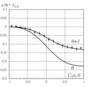
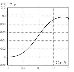
Figure 10: Left: the polarization Born asymmetry (0) and asymmetry taking into account the NLO EWC (0+1) vs scattering angle $\cos\theta$, $\mathcal{KK}$ Monte Carlo points are integrated in $\cos\theta$ bins 0.125 in width. Right: the absolute NLO correction to polarization Born asymmetry vs $\cos\theta$. Calculations are done at an $\Omega$ cut of 2 GeV. The points are the results obtained from running the $\mathcal{KK}$ Monte Carlo generator as described in the text, where the error bars represent the statistical errors from the number of Monte Carlo events generated.

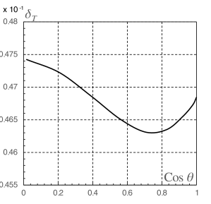
Figure 11: Left: unpolarized NLO corrected (0+1), Born (0), and their difference (1) total cross sections vs angle $a$. Right: the relative NLO correction to unpolarized total Born cross section vs $a$. Calculations are done at an $\Omega$ cut of 2 GeV. The points are the results obtained from running the $\mathcal{KK}$ Monte Carlo generator as described in the text, where the error bars represent the statistical errors from the number of Monte Carlo events generated.

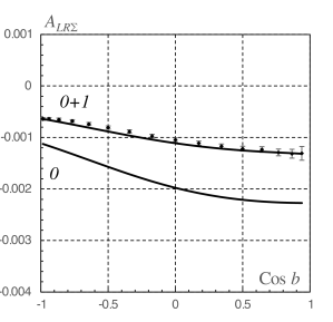
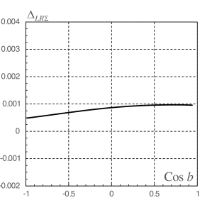
Figure 12: Left: the left-right integrated Born asymmetry (0) and asymmetry taking into account the NLO EWC (0+1) vs angle $b$ at $a=10^{\circ}$. Right: the absolute NLO correction to left-right integrated Born asymmetry vs $b$ at $a=10^{\circ}$. Calculations are done at an $\Omega$ cut of 2 GeV. The points are the results obtained from running the $\mathcal{KK}$ Monte Carlo generator as described in the text, where the error bars represent the statistical errors from the number of Monte Carlo events generated.

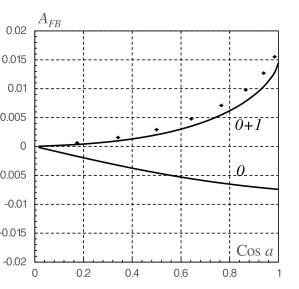
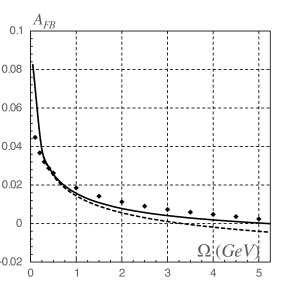
Figure 13: Left: the forward-backward Born asymmetry (0) and asymmetry taking into account the NLO EWC (0+1) vs angle $a$ at an $\Omega$ cut of 2 GeV. Right: Calculations in two approaches: SPA (dashed line) and HPA (solid line), the NLO corrected forward-backward asymmetry at $a$=30^∘. The points are the results obtained from running the $\mathcal{KK}$ Monte Carlo generator as described in the text, where the error bars represent the statistical errors from the number of Monte Carlo events generated.

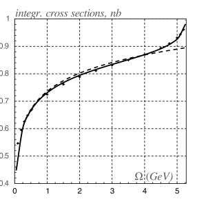
Figure 14: Calculations in two approaches: SPA (dashed line) and HPA (solid line). Left: The NLO corrected unpolarized differential cross section at $a$=$30^{\circ}$ vs $\Omega$. Right: the NLO corrected unpolarized integrated cross section at $a$=$10^{\circ}$, $b$=$170^{\circ}$ vs $\Omega$. The points are the results obtained from running the $\mathcal{KK}$ Monte Carlo generator as described in the text, where the error bars represent the statistical errors from the number of Monte Carlo events generated.

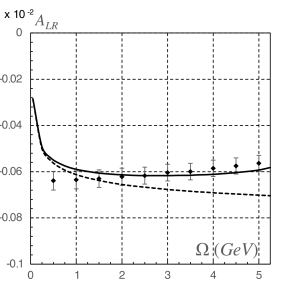
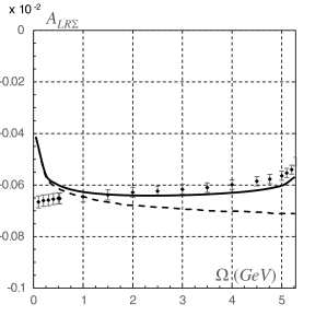
Figure 15: Calculations in two approaches: SPA (dashed line) and HPA (solid line). Left: the NLO corrected polarization asymmetry at $\theta$=90^∘, $\mathcal{KK}$ Monte Carlo integrated between 70^∘ and 110^∘. Right: the NLO corrected integrated asymmetry from $a$=$10^{\circ}$ to $b$=$170^{\circ}$. The points are the results obtained from running the $\mathcal{KK}$ Monte Carlo generator as described in the text, where the error bars represent the statistical errors from the number of Monte Carlo events generated.

Various numerical results for asymmetries and radiative corrections are presented on Figs. 9–15. Here, for the cut on energy of the emitted hard photon, in the center-of-mass system of $e^{-}$ and $e^{+}$, we used $\Omega=2.0\ \mbox{GeV}$.

As we can see on Fig.9, the correction to the unpolarized cross section related to the forward/backward kinematics is not negligible. The correction in the region $50^{\circ}\leq\theta\leq 130^{\circ}$ is linearly decreasing with its central value at $\sim 5.0\%$. It is important to note that our comparison between asymptotic and full semi-automatic results (see Tbl.1) has used only the soft-photon contribution to the unpolarized cross-section and that obviously disagrees with the values of the correction on Fig.9 (left plot), where the hard photon bremsstrahlung contribution was also included. For the L-R polarization asymmetry on Fig.10, we observe a standard dependence of the asymmetry on scattering angle. Here, as expected, the asymmetry reaches its maximum value at forward angles, which is explained by the short range interaction regime, where the parity violating $Z$-boson exchange dominates the contribution to the numerator of the asymmetry term. At backward angles we observe that the asymmetry is trending towards a zero value due to the large range interaction regime, where short range $Z$-boson exchange has a negligible contribution, and hence the entire L-R asymmetry goes to zero.

The total cross section and NLO correction, as a function of detector acceptance, are shown on Fig.11. The correction to the total cross section reaches the value of $\sim 46.8\%$, for full geometrical acceptance, and is relatively constant.

The integrated L-R asymmetry $A^{0+1}_{LR\Sigma}$ and its NLO correction $\Delta_{LR\Sigma}$ are shown on Fig.12. The maximum value of $A^{0+1}_{LR\Sigma}$ (for $a=10^{\circ}$ and $b=170^{\circ}$) is approximately equal to the average value of differential L-R asymmetry, which also corresponds to $A_{LR}^{0+1}$ at $\theta=90^{\circ}$. Results for the calculated $A^{0+1}_{FB}$ asymmetry are shown in Fig.13.

Figs.13-15 are dedicated to the sensitivity study of calculated observables to the cuts on the energy of emitted soft photons. In these plots we show dependencies of the observables on the photon’s energy cut $\Omega$, where the dashed line was obtained using the soft-photon approach only, and the solid line corresponds to the calculation with hard-photon emission.

As it can be seen, for the asymmetries, either $A_{LR}^{0+1}$, $A_{FB}^{0+1}$ or $A_{LR\Sigma}^{0+1}$, the two approaches start to deviate significantly at $\Omega\approx 0.5\ \mbox{GeV}$. This justifies the importance of inclusion of hard-photon emission calculations when it is required to provide analysis for observables such as asymmetries. However, for the various cross sections such as $d\sigma^{0+1}$, $\Sigma^{0+1}_{T}$ or $\Sigma^{0+1}_{00}$ the discrepancy between two approaches start to become visible only at $\Omega\approx 4.5\ \mbox{GeV}$, which is rather close to the maximum energy of emitted photons, $\Omega=5.2885\ \mbox{GeV}$. Since the calculations in the soft-photon approach are considerably simpler, we can rely on SPA when dealing with cross section calculations.

Comparisons with $\mathcal{KK}$ Monte Carlo:
The $\mathcal{KK}$KK Monte Carlo code is used by a number of particle physics experiments, including BaBar, Belle and Belle II, to simulate $e^{+}e^{-}\rightarrow\mu^{+}\mu^{-}(n\gamma)$ and $e^{+}e^{-}\rightarrow\tau^{+}\tau^{-}(n\gamma)$ events. In $\mathcal{KK}$, photon emission effects from the initial beams as well as outgoing fermions are calculated up to second order, including interference effects, using Coherent Exclusive Exponentiation (CEEX) CEEX and electroweak corrections using the DIZET library, which is based on the on-shell renormalization scheme DIZET . The calculations of this work are compared to those provided by $\mathcal{KK}$ version 4.19, which uses DIZET version 6.05. In order to carry out these comparisons the particle masses used in $\mathcal{KK}$ were changed to match those in Sect. IV and the Weinberg mixing angle, which is also an input to $\mathcal{KK}$, was set to the value corresponding to the on-shell value of $\sin^{2}\theta_{W}=0.221392$, as described by (13).

Two billion $e^{+}e^{-}\rightarrow\mu^{+}\mu^{-}$ events were generated with $\mathcal{KK}$ for both a left-handed polarized e^- beam and a right-handed polarized e^- beam. Each simulated event was required to produce both muons within an angular acceptance of $a=10^{\circ}$ and $b=170^{\circ}$. From the simulated events comparisons were made with each observable in Figs.9-15. For Figs.9-10 the $\mathcal{KK}$ results were binned in $\cos\theta$ with bins 0.125 in width. The mean of each bin was used to determine the $\cos\theta$ value of the points. In both of these figures the $\mathcal{KK}$ results are in agreement with our calculations. In order to obtain the differential cross section in $\mathcal{KK}$ we calculate the integrated cross section in the bin and then normalize it by the width of the bin. In Figs.11-12 the $\mathcal{KK}$ events are binned by angular acceptance. Note that as one end of the bin is fixed and the other moved to various angular cuts, some $\mathcal{KK}$ events populate multiple bins and therefore the points are not statistically independent. Using $\mathcal{KK}$ the forward-backward asymmetry was determined with two separate methods. The first method counts the events that fall in an angular acceptance between $\pm a$ and 90^∘ with a 2 GeV $\Omega$ cut, shown in Fig.13(Left). The second method counts events as a function of the $\Omega$ cut in an angular acceptance of $a=30^{\circ}$ and $90^{\circ}$, as seen in Fig.13(Right). The forward-backward asymmetry seen in Fig.13 shows an offset of a few percent between our calculations and the $\mathcal{KK}$ results. This is most likely a result of $A_{FB}$ receiving a substantial contribution from the IR-finite part of the photon bremsstrahlung terms (see Fig.8, left plot). In our case we consider only one-photon emission in initial and final states, while $\mathcal{KK}$ accounts for higher photon multiplicity when the bremsstrahlung contribution to $A_{FB}$ is calculated.

In Fig.13 we switch from angular acceptances to cuts on the energy of the emitted photon. As multiple photons are produced in $\mathcal{KK}$, not just a single photon, we define $\Omega$ as $\Omega_{KK}=\frac{\sqrt{s}}{2}\left(1-\frac{s^{\prime}}{s}\right)$, where $s$ is the square of the center-of-mass energy and $s^{\prime}$ is the square of the invariant mass of the muon pair. In Figs.14-15 the $\mathcal{KK}$ events are binned according to the $\Omega$ cut value of the event. As some events populate multiple bins as the $\Omega$ cut value is varied, this again leads to statistical correlations between bins on these plots. The level of agreement between the $\mathcal{KK}$ cross sections and the NLO corrected (0+1) cross sections can be seen in Fig.14. Fig.15 compares the $\mathcal{KK}$ results with our calculations of $A_{LR}$ as a function of the $\Omega$ cut. In order to compare our calculations of $A_{LR}$ at $\theta=90^{\circ}$ as a function of the $\Omega$ cut to those of $\mathcal{KK}$ (Fig.15(Left)), the acceptance for charged muons generated by $\mathcal{KK}$ is set to $70^{\circ}<\theta<110^{\circ}$, a region over which the $A_{LR}$ dependence on $\cos\theta$ is linear to a good approximation (see Fig.10). Note that, again, the point-to-point correlations are large. From Fig.15(Right), it is evident that in the region 1 GeV$<\Omega<$3 GeV the $\mathcal{KK}$ results integrated over $10^{\circ}<\theta<170^{\circ}$ are in good agreement with the HPA calculation, within the $\mathcal{KK}$ statistical uncertainties. This statistical uncertainty arises from the finite number of events generated by $\mathcal{KK}$ for each of the two e^- polarization states. Accounting for the numbers of $\mathcal{KK}$ events from each sample that survive the acceptance and $\Omega$ requirements, the absolute $\mathcal{KK}$ statistical uncertainty on $A_{LR}$ is $\pm 1.9\times 10^{-5}$.

It is evident that at low values of $\Omega$ there is significant disagreement between $\mathcal{KK}$ and the SPA and HPA treatments. This is a result of the fact that $\mathcal{KK}$ addresses infrared divergences via exponentiation whereas in the SPA and HPA treatments, the infrared divergences persist.

V Sensitivity Study

We next study the sensitivities of the observables $A^{0+1}_{LR\Sigma}$ (65) and $A^{0+1}_{FB}$ (68) to the effective weak mixing angle $(\bar{s}_{W}^{2}\equiv\sin^{2}\theta_{W}^{eff})$ and vector part of the $Z$-boson to fermion coupling ($v^{Z}_{eff}=I_{3}-2Q_{g}\bar{s}_{W}^{2}$).

In order to represent the $e^{+}e^{-}\rightarrow\mu^{+}\mu^{-}$ matrix element with the simple effective Born-like amplitude, we can use leading order low energy one-loop oblique corrections to the Born matrix element. Overall we can write for the QED and electroweak parts Hollik :

$$M_{\gamma} = \frac{\alpha(s)Q_{e}Q_{\mu}}{s}\left(\bar{v}_{e}\gamma_{\nu}u_{e}\right)\left(\bar{u}_{\mu}\gamma^{\nu}v_{\mu}\right),$$

$$M_{Z} = \frac{G_{\mu}}{\sqrt{2}}\kappa\frac{m_{Z}^{2}}{s-m_{Z}^{2}+i\frac{s}{m_{Z}}\Gamma_{Z}}\left(\bar{v}_{e}\gamma_{\nu}\left[I^{3}_{e}-2\bar{s}_{W}^{2}(s)Q_{e}-I^{3}_{e}\gamma_{5}\right]u_{e}\right)\left(\bar{u}_{\mu}\gamma^{\nu}\left[I^{3}_{\mu}-2\bar{s}_{W}^{2}(s)Q_{\mu}-I^{3}_{\mu}\gamma_{5}\right]v_{\mu}\right).$$

Here $\alpha(s)$ represents the running value of fine structure constant, defined as

$$\alpha(s) = \frac{\alpha}{1+\Re\left[\hat{\Sigma}_{\gamma\gamma}(s)\right]/s},$$

and $\bar{s}_{W}^{2}(s)$ defines the effective running Weinberg mixing angle through the following expression

$$\bar{s}_{W}^{2}\left(s\right) = s_{W}^{2}-s_{W}c_{W}\frac{\Re\left[\hat{\Sigma}_{\gamma Z}(s)\right]}{s+\Re\left[\hat{\Sigma}_{\gamma\gamma}(s)\right]}.$$ (72)

Parameter $\kappa$, is defined based on relationship to expression (58) in the following way:

$$\kappa = \frac{1-\Delta r}{1+\Re\left[\frac{\partial}{\partial s}\hat{\Sigma}_{ZZ}(s)\right]}.$$ (73)

The effective mixing angle is frequently used as one of the primary parameters in precision electroweak physics and here we study the dependencies of $A^{0+1}_{LR\Sigma}$ and $A^{0+1}_{FB}$ on $\bar{s}^{2}_{W}$. To start with, we show on Tbl.2, $\bar{s}_{W}^{2}(s)$ computed in different renormalization schemes at zero and $Z$-pole kinematics. Our calculated on-shell values of $\bar{s}_{W}^{2}(s)$ compare favorably with those calculated in the $\overline{MS}$ scheme, as reported in the PDG $\overline{MS}$.

$s$ ($\mbox{GeV}^{2})$	$\bar{s}_{W,{\rm on-shell}}^{2}$	$\bar{s}_{W,\overline{MS}}^{2}$, PDG(2016)
$0$	0.23821	0.23857
$m_{Z}^{2}$	0.23124	0.2313

Table 2: Results of $\bar{s}_{W}^{2}$ in on-shell and $\overline{MS}$ renormalization schemes.

For the kinematics relevant to the Belle II experiment, $\sqrt{s}=10.58$ GeV, the on-shell effective value of $\bar{s}_{W}^{2}(s)$ is equal to $0.23413$. In order to study the sensitivity of the polarization asymmetry to the variation of $\bar{s}_{W}^{2}(s)$, we can simply vary the value of $m_{W}$, then calculating $\bar{s}_{W}^{2}(s)$ and asymmetries, we construct parametric dependencies of the asymmetry on $\bar{s}_{W}^{2}(s)$ or $v^{Z}_{eff}$. It is important to note that in the analysis of the sensitivity of the asymmetries we took the cut on the bremsstrahlung photons at $2.0\ \mbox{GeV}$.

In order to evaluate the experimental asymmetry uncertainties that feed into the sensitivities, we make the following reasonable assumptions regarding pertinent experimental parameters that potentially can be achieved at Belle II/SuperKEKB if there is an upgrade that introduces polarization:

• the electron beam polarization is $p_{B}=0.7000\pm 0.0035$, the positron beam is unpolarized.

• $p_{B}$ can measured with 0.5% precision, and this dominates the systematic error on $A_{LR}$.

• $A_{FB}$ can be measured with an absolute systematic uncertainty of 0.005.

• Belle II collects 20 ab^-1 of data with the electron beam polarization and selects $e^{-}e^{+}\rightarrow\mu^{-}\mu^{+}(\gamma)$ events with 50% efficiency.

• The average $\sqrt{s}$, which has a root-mean-square (RMS) spread of 5 MeV BelleIITDR , is known to $\pm 1.2~{}$MeV of the peak of the $\Upsilon(4S)$ resonance.

With such parameters we can expect an absolute statistical uncertainty on both $A_{FB}$ and $A_{LR}$ of $9.4\times 10^{-6}$. This gives a total uncertainty on $A_{LR\Sigma}$(with $b=170^{\circ}$) of $\pm$0.0000094(stat)$\pm$0.0000030(syst)=$\pm$0.0000097(total). The error is dominated by the statistical uncertainty and gives a relative uncertainty on $A_{LR\Sigma}$ of 1.6%. The total uncertainty on $A_{FB}$(with $a=10^{\circ}$; $b=170^{\circ}$) is $\pm$ 0.0050 (total). In this case, the uncertainty is completely dominated by the systematic uncertainty and gives a relative error on $A_{FB}$ of 9.4%.

The reason for this difference in relative uncertainties is that the systematic error on $A_{LR}$ scales as the relative error because $p_{B}$ is a multiplicative correction needed for the measurement and has no other large systematic error since essentially all other detector systematic errors cancel. On the other hand, for $A_{FB}$ the dominant systematic errors arise in the detector and do not fully cancel: it is necessary to measure the angles and forward and backward acceptances, the boost to transform into the CM frame, and understand any charge asymmetries in the detector. As these are systematic uncertainties in the detector asymmetries, they are absolute uncertainties on $A_{FB}$.

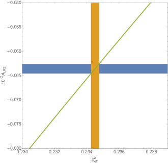
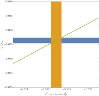
Figure 4: Dependence of the integrated left-right asymmetry on the effective Weinberg mixing angle (left) at $\sqrt{s}=10.58$ GeV and vector part of the electroweak coupling (right). Horizontal bands show the central value of $A^{0+1}_{LR\Sigma}=-0.00063597$ determined with the cut on soft-photons at $2.0\ \mbox{GeV}$. The width of the band corresponds to the $\pm 0.0000097$ uncertainty on the central value of $A^{0+1}_{LR\Sigma}$.

Fig.4 shows a linear dependence of $A^{0+1}_{LR\Sigma}$ on $\bar{s}_{W}^{2}\ (s=10.58^{2}\ \mbox{GeV}^{2})$. That is evident from the fact that the polarization asymmetry is proportional to the interference term: $2\Re\left[M_{\gamma}M_{Z}^{*}\right]$, which is linearly proportional to $\bar{s}_{W}^{2}(s)$. As it can be seen from Fig.4, the absolute uncertainty for $A^{0+1}_{LR\Sigma}$ equal to $\pm 0.000097$, translates into an uncertainty of 0.21% on $\bar{s}_{W}^{2}(s)$ at $s=10.58^{2}\ \mbox{GeV}^{2}$.

In general the on-shell extraction of $\bar{s}_{W}^{2}(s)$ from an experimental polarization asymmetry could be done by determining the effective $m_{W}$ from the measured $A^{0+1}_{LR\Sigma}$, and then determine $\bar{s}_{W}^{2}(s)$ for that specific effective $m_{W}$ from equation (72).

It is known that in the time-like region, the value of $\bar{s}_{W}^{2}(s)$ changes rapidly near resonances. Although we have not included the effect of hadronic resonances in our treatment, we can estimate the impact of such an effect on the precision of an asymmetry measurement made at the peak of the $\Upsilon(4S)$ resonance using Fig. 1 of referenceJegerlehner2017 . From that figure, $\sin^{2}\theta_{W}$ changes by approximately 0.003 over the 20.5 MeV full width of the $\Upsilon(4S)$ resonance and therefore there is a sensitivity of $\Delta_{\sin^{2}\theta_{W}}/\Delta_{\sqrt{s}}=0.00015$/MeV in the region of the peak of the $\Upsilon(4S)$ resonance. As $\sqrt{s}$ is known to $\pm$1.2 MeV, in the interpretation of the integrated $A_{LR}$ measurement in terms of $\bar{s}_{W}^{2}(s)$, this translates into an uncertainty on $\bar{s}_{W}^{2}(s)$ of approximately $0.00018$, or 0.08$\%$, which contributes a small additional uncertainty: adding this in quadrature with the 0.21$\%$ coming from the other uncertainties yields a total uncertainty on $\bar{s}_{W}^{2}(s)$ of 0.22$\%$. We note that this uncertainty will be common to measurements from each fermion species and therefore will cancel in evaluations of fermion universality of the weak mixing angle performed with $A_{LR\Sigma}$ at Belle II.

In a similar fashion we can study the sensitivity of the forward-backward asymmetry to the variations of $\bar{s}_{W}^{2}(s)$. The Fig.5 shows the similar dependence of $A^{0+1}_{FB}$ on $\bar{s}_{W}^{2}(s)$, but with a substantially smaller slope when compared to Fig.4.

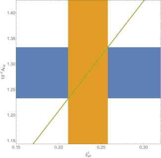
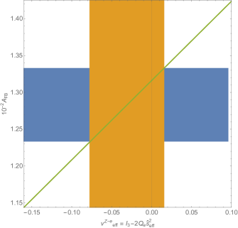
Figure 5: Forward-backward asymmetry for the $a=10^{\circ}$ and $b=170^{\circ}$ as a function of $\bar{s}_{W}^{2}(s)$. Horizontal band shows the central value of $A^{0+1}_{FB}=0.01283$ determined with the cut on hard-photons at $2.0\ \mbox{GeV}$. Width of the band corresponds to the 1% uncertainty on the central value of $A^{0+1}_{FB}$.

Although the numerical value of $A^{0+1}_{FB}$ is much larger than $A^{0+1}_{LR\Sigma}$, it’s sensitivity to $\bar{s}_{W}^{2}(s)$ is rather low. This translates to an uncertainty of 19.8% on $\bar{s}_{W}^{2}(s)$, if we consider $\pm 0.00050$ uncertainty in $A^{0+1}_{FB}$.

Clearly $A^{0+1}_{FB}$ contains substantial contributions, which are not sensitive to parity-violating physics. At this point we would like to determine the most dominant contributions to $A^{0+1}_{FB}$ and their nature. We will start with the basic definition of various QED and Weak contributions in the forward-backward asymmetry:

$$A^{0+1}_{FB} =\frac{\Sigma_{F}^{{0+1}}-\Sigma_{B}^{{0+1}}}{\Sigma_{F}^{{0+1}}+\Sigma_{B}^{{0+1}}}=\frac{\Gamma_{FB}^{{0+1}}}{\Sigma_{T}^{0+1}}$$ (74)

The denominator of (74), is defined as a total integrated unpolarized cross section including one-loop corrections. We will keep this part of $A^{0+1}_{FB}$ unmodified. This way contributions to the asymmetry are additive. As for the numerator of $A^{0+1}_{FB}$, it will be divided into Born, various infrared finite NLO, and soft-bremsstrahlung contributions. More specifically:

$$\Gamma_{FB}^{0+1} =\Gamma_{FB}^{0}+\Gamma_{FB}^{\gamma-SE(\gamma)}+\Gamma_{FB}^{\gamma-TR(\gamma)}+\Gamma_{FB}^{\gamma-BB(\gamma)}+\Gamma_{FB}^{\gamma-SE(Z)}+\Gamma_{FB}^{\gamma-TR(Z)}+\Gamma_{FB}^{\gamma-BB(Z)}+$$

$$\Gamma_{FB}^{Z-SE(\gamma)}+\Gamma_{FB}^{Z-TR(\gamma)}+\Gamma_{FB}^{Z-BB(\gamma)}+\Gamma_{FB}^{Z-SE(Z)}+\Gamma_{FB}^{Z-TR(Z)}+\Gamma_{FB}^{Z-BB(Z)}+\Gamma_{FB}^{soft}$$ (75)

Here, $\Gamma_{FB}^{0}$ is the forward-backward Born contribution to the numerator of $A^{0+1}_{FB}$, and $\Gamma_{FB}^{\gamma-SE(\gamma)}$ (for example) and corresponds to the interference term between Born QED and $\gamma-\gamma$ Self-Energies (SE). Furthermore TR and BB stand for Triangle and Box type graphs, respectively.

Our starting point is to show Born and fully corrected forward-backward asymmetries. We do this for both renormalization conditions, based on hollik and Denner .

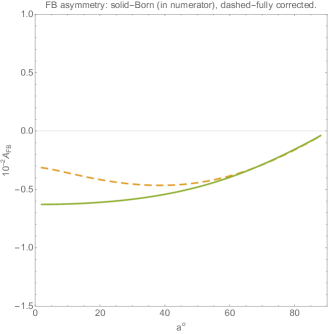
Figure 6: Born (first term in Eq.75) and fully corrected $A^{0+1}_{FB}$. Born is represented by solid line, and corrected $A^{0+1}_{FB}$ is shown by dashed line.

Results on Fig.6 are represented by the infrared finite parts of virtual and soft-bremsstrahlung corrections only. That would also be true for all partial NLO contributions appearing in (75). We have observed practically zero contributions coming from $\Gamma_{FB}^{\gamma-SE(\gamma)},\Gamma_{FB}^{\gamma-TR(\gamma)},\Gamma_{FB}^{\gamma-SE(Z)},\Gamma_{FB}^{\gamma-BB(Z)},\Gamma_{FB}^{Z-SE(\gamma)},\Gamma_{FB}^{Z-SE(Z)},\Gamma_{FB}^{Z-TR(Z)},\Gamma_{FB}^{Z-BB(\gamma)}$ and $\Gamma_{FB}^{Z-BB(Z)}$ terms in (75). This implies that contributions coming from all types of self-energies and electroweak ($\gamma-Z,\,Z-Z$ and $W-W$) boxes are negligible, and can be disregarded. It is important to note that generally electroweak self-energies or vertex correction graphs are not gauge invariant and hence their independent contributions have no physical meaning. However, for the forward-backward asymmetry this can be bypassed, since gauge dependent contributions largely cancel out even for separate parts, such as self-energies or vertex correction graphs. We have verified this by comparing self-energies (or triangles) contributions in the different renormalization conditions (Denner and Hollik) and found that the results are identical. At this point we only show contributions which are substantial and can not be avoided in the calculations of $A^{0+1}_{FB}$.

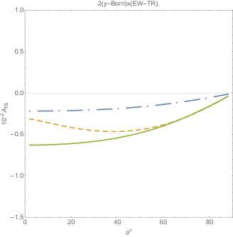
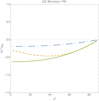
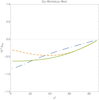
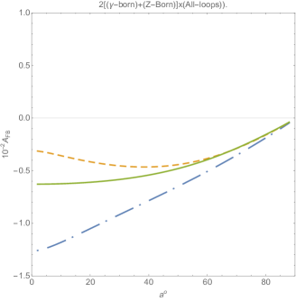
Figure 7: Various contributions to $A_{FB}$. On all graphs, solid green line corresponds to Born contribution (in numerator of $A_{FB}$), dashed yellow line is fully corrected asymmetry and dot-dashed blue shows various NLO parts of $A_{FB}$.

As we can see from Fig.7 (two top graphs), we have identical (symmetrical) contributions from interference terms, such as: $2\Re[M_{0}^{\gamma}M_{one-loop}^{EW-TR}]$ and $\Re[M_{0}^{Z}M_{one-loop}^{\gamma-TR}]$. The biggest contribution comes from the interference term between $\gamma$-Born and $\gamma\gamma$-Box (see Fig.7, second row, left). Overall, all one-loop contributions are systematically additive and the result is shown on Fig.7, second row, right graph. Since it is clear now that the addition of one-loop contributions (blue, dot-dashed curve) and Born (green, solid curve) term would not reproduce the full result for $A^{0+1}_{FB}$, we turn our attention to IR finite terms of soft-photon bremsstrahlung.

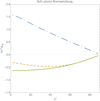
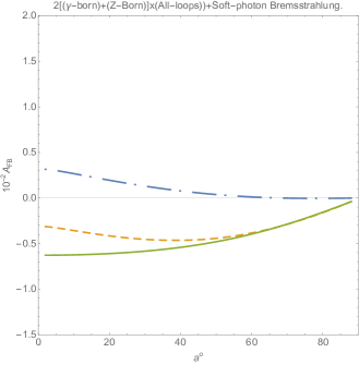
Figure 8: IR finite soft-photon bremsstrahlung (left plot) and total correction (right plot) to the numerator of the asymmetry. Solid green line corresponds to Born contribution (in numerator of $A_{FB}$), dashed yellow line is fully corrected asymmetry and dot-dashed blue shows various NLO parts of $A_{FB}$.

It is clearly visible on Fig.8 (left) that the bremsstrahlung contribution largely cancels out one-loop results and produce the correction, shown on Fig.8 (right and blue dot-dashed curve). The addition of the one-loop correction (Fig. 8, left and blue dot-dashed curve ) and Born result (solid green curve on the same plot) produce the final result for $A^{0+1}_{FB}$ (dashed yellow curve). One of the possible explanations for such a large cancellation could be found in the fact that both of the IR finite parts of virtual one-loop correction and soft-photon bremsstrahlung contain collinear divergent terms, which cancel out in the final result.

Overall we conclude that $A^{0+1}_{LR\Sigma}$ is the observable most sensitive to the effective electroweak parameters. As such, in order to search for physics beyond the Standard Model at the precision frontier of neutral-current measurements, it is crucial to have polarized electron beams in Belle II/SuperKEKB in order to measure $A^{0+1}_{LR\Sigma}$.

VI Conclusion

In this paper we compare the results for the full set of one-loop EWC to parity violating polarization and forward-backward asymmetries at the Belle II/SuperKEKB CM energy obtained by different methods. The soft photon approximation using an exact semi-automatic approach is validated by an asymptotic approach with simplifications giving a compact form. We take under full control the bremsstrahlung process and compare results for the soft and hard photon calculations. We also evaluate the sensitivity to the variation of $\bar{s}_{W}^{2}$ for both polarization and forward-backward asymmetries. We find that the highest sensitivity is achieved for the measurements using $A_{LR\Sigma}$ with a polarized electron beam. In addition, we have analyzed various NLO contributions to the IR finite part of $A_{FB}^{0+1}$. As a result, we found that the large contribution arising from interference terms between $\{\gamma,\ Z\}$-Born, $\{\gamma-\gamma\}$-Box, and $\{\gamma,\ Z\}$-Triangle graphs are compensated by the IR finite part of the soft-photon bremsstrahlung contribution and that self-energies, although important for the overall cross-sections, cancel out for the forward-backward asymmetry and therefore have an overall negligible contribution to that asymmetry. A comparison is also made with the $\mathcal{KK}$ Monte Carlo generator for the $A_{LR}$ and $A_{FB}$ asymmetries. Where infrared divergencies are small, our current calculations are in good agreement with those of the $\mathcal{KK}$ Monte Carlo.

We plan to broaden these studies to include left-right asymmetries in $e^{+}e^{-}$ collisions for Bhabha scattering and for massive final-state fermions (tau leptons, charm and bottom quarks), where the negligible-mass assumption is not valid. In order to further reduce the theoretical uncertainties, our next step is to include the two-loop EWC in the on-shell renormalization scheme, and compare these to the calculation in the $\overline{MS}$ scheme. Nonetheless, the results of this paper demonstrate that the Standard Model predictions for $A_{LR}$ at 10.58 GeV, and consequently the weak mixing angle at that energy, are already under excellent theoretical control and provide encouragement to upgrade SuperKEKB with a polarized e^- beam in order to provide a new tool in the search for physics beyond the Standard Model.

VII ACKNOWLEDGMENTS

We are grateful to Eduard Alekseevich Kuraev for stimulating discussions. V.Z. thanks the Acadia University (Wolfville, Canada) and Memorial University (Corner Brook, Canada) for hospitality. This work was supported by the Belarusian State Program of Scientific Research “Convergence-2020” and the Natural Sciences and Engineering Research Council of Canada.

Figure 9: Left: unpolarized NLO corrected (0+1), Born (0), and their difference (1) differential cross sections vs scattering angle $\theta$. Right: the relative NLO correction to unpolarized Born cross section vs $\theta$. Calculations are done at an $\Omega$ cut of 2 GeV. The points are the results obtained from running the $\mathcal{KK}$ Monte Carlo generator as described in the text, where the error bars represent the statistical errors from the number of Monte Carlo events generated.

References

- (1) Belle II Technical Design Report, Belle II Collaboration: T. Abe et al., arXiv:1011.0352 [physics.ins-det], KEK Report 2010-1, October 2010.
- (2) SuperB Technical Design Report, SuperB Collaboration: M. Baszczyk et al., arXiv:1306.5655 [physics.ins-det], INFN-13-01-PI, LAL-13-01, SLAC-R-1003.
- (3) J.M. Roney, “Precision electroweak measurements at SuperB with polarised beams”, ICHEP2012, Melbourne (2012).
- (4) M. Baak et al. [Gfitter Group Collaboration], Eur.Phys.J. C 74 3046 (2014).
- (5) M. Böhm and W. Hollik, Nucl. Phys. B 204, 45 (1982).
- (6) W. Hollik, Fortschr. Phys. 38, 165 (1990).
- (7) M. Bohm, W. Hollik, Z. Phys. C 23, 31 (1984).
- (8) V.A. Novikov, L.B. Okun, M.I. Vysotsky, Nucl. Phys. B 397, 35 (1993).
- (9) G. Montagna et al., Comput. Phys. Commun. 117, 278 (1999).
- (10) D. Bardin et al., Comput. Phys. Commun. 133, 229 (2001).
- (11) D.Yu. Bardin, S. Rieman, T. Rieman, Z. Phys. 32, 121 (1986).
- (12) S. Jadach, B.F.L. Ward and Z. Was, Comput.Phys.Commun. 130 (2000); S. Jadach, B.F.L. Ward and Z. Was, Phys. Rev. D 63, 113009 (2001).
- (13) A. Andonov et al., Phys. Part. Nucl. 34, 1125 (2003).
- (14) T. Hahn, arXiv:hep-ph/0012260v2 (2000).
- (15) T. Hahn, M. Perez-Victoria, Comput. Phys. Commun. 118, 153 (1999).
- (16) J. Vermaseren, math-ph/0010025 (2000).
- (17) M. Böhm, H. Spiesberger, and W. Hollik, Fortschr. Phys. 34, 687 (1986).
- (18) A. Denner, Fortsch. Phys. 41, 307 (1993).
- (19) V.A. Zykunov, Yad. Fiz. 69, 1557 (2006) [Phys. At. Nucl. 69, 1522 (2006)].
- (20) A. Aleksejevs et al., Phys. Rev. D 82, 093013 (2010).
- (21) F. Berends, K. Gaemer, R. Gastmans, Nucl. Phys. B 57, 381 (1973).
- (22) G. ’t Hooft and M. Veltman, Nucl. Phys. B 153, 365 (1979).
- (23) E.A. Kuraev, N. R. Merenkov, and V. S. Fadin, Yad. Fiz. 45, 782 (1987).
- (24) P.G. Lepage, J. Comput. Phys. 27, 192 (1978).
- (25) V.A. Zykunov, Eur. Phys. J. direct C 3 (2001) 9 [hep-ph/0107059].
- (26) C. Patrignani et al. (Particle Data Group), Chin. Phys. C, 40, 100001 (2016).
- (27) F. Jegerlehner, J. Phys. G. 29 101 (2003) [hep-ph/0104304].
- (28) Jadach, S. and Ward, B. F. L. and Wa¸s, Z., Phys. Rev. D 63, 113009.
- (29) D. Y. Bardin, M. S. Bilenky, T. Riemann, M. Sachwitz and H. Vogt, Comput. Phys. Commun. 59, 303 (1990). doi:10.1016/0010-4655(90)90179-5
- (30) W. Hollik, DESY 88-188, (1988).
- (31) A. Ferroglia, G. Ossola, A. Sirlin, EPJC., 10.1140, (2003).
- (32) F. Jegerlehner, arXiv:1711.06089v1 [hep-ph] (2017).