Arbitrary-order functionally fitted energy-diminishing methods for gradient systems

Abstract

It is well known that for gradient systems in Euclidean space or on a Riemannian manifold, the energy decreases monotonically along solutions. In this letter we derive and analyse functionally fitted energy-diminishing methods to preserve this key property of gradient systems. It is proved that the novel methods are unconditionally energy-diminishing and can achieve damping for very stiff gradient systems. We also show that the methods can be of arbitrarily high order and discuss their implementations. A numerical test is reported to illustrate the efficiency of the new methods in comparison with three existing numerical methods in the literature.

Keywords: gradient systems, energy-diminishing methods, functionally fitted methods, arbitrary-order methods

MSC:65L05

1 Introduction

In this letter, we investigate the following gradient systems in coordinates:

$$G(y(t))\dot{y}(t)=-\nabla U(y(t)),\quad y(0)=y_{0}\in\mathbb{R}^{d},\quad t\in[0,T],$$ (1)

where $U(y):\mathbb{R}^{d}\rightarrow\mathbb{R}$ is a potential function and the symmetric matrix $G(y)$ is assumed to satisfy

$$v^{\intercal}G(y)v\geq v^{\intercal}\Gamma v>0$$

for all vectors $v\neq 0.$ Here $\Gamma$ is a fixed positive definite matrix.

Gradient systems frequently arise in a wide variety of applications both in a finite-dimensional and infinite-dimensional setting. There are many examples of this system (see, e.g. [1, 3, 4, 17, 18, 19, 20]) such as models in quantum systems, in differential geometry, in image processing, and in material science. A fundamental and key property of gradient systems is that along every exact solution of (1), one has

$$\frac{d}{dt}U(y(t))=\nabla U(y(t))^{\intercal}\dot{y}(t)=-\dot{y}(t)^{\intercal}G(y(t))\dot{y}(t)\leq 0,$$

which shows that $U(y(t))$ is monotonically decreasing with $t$. The monotonicity is true with strict inequality except at stationary points of $U$. The aim of this letter is to formulate and analyse a novel kind of methods preserving this monotonicity in the numerical treatment, i.e., after one step of the method starting from $y_{0}$ with a time step $h$ one would have

$$U(y_{1})\leq U(y_{0}).$$

In order to get methods with this property, Hairer and Lubich analysed various energy-diminishing methods in [6]. They showed that implicit Euler method has this property but it is only of order one. Algebraically stable Runge-Kutta methods were proved to reduce the energy in each step under a mild step-size restriction, which means that Runge-Kutta methods are not unconditionally energy-diminishing. They also showed that discrete-gradient methods, averaged vector field (AVF) methods and AVF collocation methods are unconditionally energy-diminishing, but cannot achieve damping for very stiff gradient systems. In this letter, we will derive a novel kind of methods which can be of arbitrarily high order. Moreover, the methods will be shown that they are unconditionally energy-diminishing and are strongly damped even for very stiff gradient systems.

The rest of this letter is organised as follows. In Section 2, we derive the novel methods and prove that they are unconditionally energy-diminishing for gradient systems. The unconditionally damping property is analysed in Section 3. We study the order of the methods in Section 4. Section 5 is devoted to the implementation issue. In Section 6, a numerical test is carried out to demonstrate the excellent qualitative behavior. Section 7 focuses on the concluding remarks.

2 Functionally fitted energy-diminishing methods

In order to formulate the novel methods, we will use the functionally fitted technology, which is a popular approach to constructing efficient and effective methods in scientific computing (see, e.g. [11, 22]). To this end, define a function space $Y$=span$\left\{\varphi_{0}(t),\ldots,\varphi_{r-1}(t)\right\}$ on $[0,T]$ by (see [11])

$$Y=\left\{w:w(t)=\sum_{i=0}^{r-1}\varphi_{i}(t)W_{i},\ t\in I,\ W_{i}\in\mathbb{R}^{d}\right\},$$

where $\{\varphi_{i}(t)\}_{i=0}^{r-1}$ are sufficiently smooth and linearly independent on $[0,T]$. In this letter, we consider two finite-dimensional function spaces $Y$ and $X$ as follows

$$Y=\text{span}\left\{\varphi_{0}(t),\ldots,\varphi_{r-1}(t)\right\},\quad X=\text{span}\left\{1,\int_{0}^{t}\varphi_{0}(s)ds,\ldots,\int_{0}^{t}\varphi_{r-1}(s)ds\right\}.$$

Choose a stepsize $h$ and define the function spaces $Y_{h}$ and $X_{h}$ on $[0,1]$ by

$$Y_{h}=\text{span}\left\{\tilde{\varphi}_{0}(\tau),\ldots,\tilde{\varphi}_{r-1}(\tau)\right\},\quad X_{h}=\text{span}\left\{1,\int_{0}^{\tau}\tilde{\varphi}_{0}(s)ds,\ldots,\int_{0}^{\tau}\tilde{\varphi}_{r-1}(s)ds\right\},$$

where $\tilde{\varphi}_{i}(\tau)=\varphi_{i}(\tau h),\ \tau\in[0,1]$ for $i=0,1,\ldots,r-1$. We remark that for all the functions throughout this letter, the notation $\tilde{f}(\tau)$ is referred to $f(\tau h)$.

We will use a projection $\mathcal{P}_{h}$ in the formulation of the new methods. It was defined in [11] and we summarise it here.

Definition 1

(See [11]) Let $\mathcal{P}_{h}\tilde{w}$ be a projection of $\tilde{w}$ onto $Y_{h}$, where $\tilde{w}(\tau)$ is a continuous $\mathbb{R}^{d}$-valued function on $[0,1]$. The definition of $\mathcal{P}_{h}\tilde{w}$ is given by

$$\langle\tilde{v}(\tau),\mathcal{P}_{h}\tilde{w}(\tau)\rangle=\langle\tilde{v}(\tau),\tilde{w}(\tau)\rangle\quad\text{for any}\ \ \tilde{v}(\tau)\in Y_{h},$$

where the inner product $\langle\cdot,\cdot\rangle$ is defined by

$$\langle\tilde{w}_{1},\tilde{w}_{2}\rangle=\langle\tilde{w}_{1}(\tau),\tilde{w}_{2}(\tau)\rangle_{\tau}=\int_{0}^{1}\tilde{w}_{1}(\tau)\cdot\tilde{w}_{2}(\tau)d\tau.$$

Here $\tilde{w}_{1}$ and $\tilde{w}_{2}$ are two integrable functions (scalar-valued or vector-valued) on $[0,1]$, and ‘$\cdot$’ denotes the entrywise multiplication operation if they are both vector-valued functions.

The following property of $\mathcal{P}_{h}$ will also be useful in this letter, which has been proved in [11].

Lemma 1

(See [11]) The projection $\mathcal{P}_{h}\tilde{w}$ can be explicitly expressed as

$$\mathcal{P}_{h}\tilde{w}(\tau)=\langle P_{\tau,\sigma},\tilde{w}(\sigma)\rangle_{\sigma},$$

where

$$P_{\tau,\sigma}=\sum_{i=0}^{r-1}\tilde{\psi}_{i}(\tau)\tilde{\psi}_{i}(\sigma),$$

and $\left\{\tilde{\psi}_{0},\ldots,\tilde{\psi}_{r-1}\right\}$ is a standard orthonormal basis of $Y_{h}$ under the inner product $\langle\cdot,\cdot\rangle$.

Based on these preliminaries, we are in a position to present the scheme of functionally fitted energy-diminishing methods.

Definition 2

Choose a stepsize $h$ and consider a function $\tilde{u}\in X_{h}$ with $\tilde{u}(0)=y_{0}$, satisfying

$$G(\tilde{u}(\tau))\tilde{u}^{\prime}(\tau)=-\mathcal{P}_{h}\big{(}\nabla U(\tilde{u}(\tau))\big{)}.$$ (2)

The numerical approximation after one step is defined by $y_{1}=\tilde{u}(1).$ We call this method as functionally-fitted energy-diminishing method and denote it by FFED.

Theorem 1

The FFED method (2) reduces the energy of gradient systems (1), i.e., $U(y_{1})\leq U(y_{0}).$ This means that our FFED method (2) is unconditionally energy-diminishing.

Proof According to the definitions of $X_{h}$ and $Y_{h}$, we know that if $\tilde{u}(\tau)\in X_{h}$, then one has $\tilde{u}^{\prime}(\tau)\in Y_{h}$. From the definition of $\mathcal{P}_{h}$, it follows that

$$\int_{0}^{1}\tilde{u}^{\prime}(\tau)_{i}\mathcal{P}_{h}\big{(}\nabla U(\tilde{u}(\tau))\big{)}_{i}d\tau=\int_{0}^{1}\tilde{u}^{\prime}(\tau)_{i}\big{(}\nabla U(\tilde{u}(\tau))\big{)}_{i}d\tau,\quad i=1,2,\ldots,d,$$

where $(\cdot)_{i}$ denotes the $i$th entry of a vector. Then, we arrive at

$$\int_{0}^{1}\tilde{u}^{\prime}(\tau)^{\intercal}\mathcal{P}_{h}\big{(}\nabla U(\tilde{u}(\tau))\big{)}d\tau=\int_{0}^{1}\tilde{u}^{\prime}(\tau)^{\intercal}\nabla U(\tilde{u}(\tau))d\tau.$$

Therefore, it is obtained that

$$U(y_{1})-U(y_{0})=\int_{0}^{1}\frac{d}{d\tau}U(\tilde{u}(\tau))d\tau=h\int_{0}^{1}\tilde{u}^{\prime}(\tau)^{\intercal}\nabla U(\tilde{u}(\tau))d\tau=h\int_{0}^{1}\tilde{u}^{\prime}(\tau)^{\intercal}\mathcal{P}_{h}\big{(}\nabla U(\tilde{u}(\tau))\big{)}d\tau.$$

Inserting the scheme (2) into this formula yields

$$U(y_{1})-U(y_{0}) =-h\int_{0}^{1}\tilde{u}^{\prime}(\tau)^{\intercal}G(\tilde{u}(\tau))\tilde{u}^{\prime}(\tau)d\tau\leq 0.$$

3 Unconditionally damping property

In this section, we consider the potential $U$ of the form

$$U(y)=\dfrac{1}{2}y^{\intercal}Ay+V(y),$$ (3)

where the function $V$ is twice continuously differentiable and the matrix $A$ is symmetric positive semi-definite and of arbitrarily large norm. In this case, (1) is a stiff gradient system. This kind of stiff systems arise from the spatial discretization of Cahn–Hilliard and Allen–Cahn partial differential equations (see, e.g. [2, 5]). Many effective methods have been derived for this stiff gradient system with a constant matrix $G$ and we refer to [7, 8, 10, 12, 21, 22, 23, 24, 25] for example.

The FFED method (2) for solving this stiff gradient system is defined as follows.

Definition 3

We consider a function $\tilde{u}\in X_{h}$ with $\tilde{u}(0)=y_{0}$, satisfying

$$G(\tilde{u}(\tau))\tilde{u}^{\prime}(\tau)+A\tilde{u}(\tau)=-\mathcal{P}_{h}\big{(}\nabla V(\tilde{u}(\tau))\big{)},\qquad y_{1}=\tilde{u}(1).$$ (4)

This method is denoted by EFFED.

Theorem 2

The EFFED method (4) reduces the energy of the stiff gradient system (1) with (3), i.e., $U(y_{1})\leq U(y_{0}).$

Proof  This proof is similar to that of Theorem 1. For any $\tilde{w}(\tau)\in Y_{h}$, it is easy to prove that

$$\int_{0}^{1}\tilde{w}(\tau)^{\intercal}G(\tilde{u}(\tau))\tilde{u}^{\prime}(\tau)d\tau=-\int_{0}^{1}\tilde{w}(\tau)^{\intercal}A\tilde{u}(\tau)d\tau-\int_{0}^{1}\tilde{w}(\tau)^{\intercal}\mathcal{P}_{h}\big{(}\nabla V(\tilde{u}(\tau))\big{)}d\tau$$ (5)

$$=-\int_{0}^{1}\tilde{w}(\tau)^{\intercal}A\tilde{u}(\tau)d\tau-\int_{0}^{1}\tilde{w}(\tau)^{\intercal}\nabla V(\tilde{u}(\tau))d\tau=-\int_{0}^{1}\tilde{w}(\tau)^{\intercal}\nabla U(\tilde{u}(\tau))d\tau.$$

Considering $\tilde{u}^{\prime}(\tau)\in Y_{h}$ and letting $\tilde{w}(\tau)=\tilde{u}^{\prime}(\tau)$ in (5), we obtain

$$\int_{0}^{1}\tilde{u}^{\prime}(\tau)^{\intercal}G(\tilde{u}(\tau))\tilde{u}^{\prime}(\tau)d\tau=-\int_{0}^{1}\tilde{u}^{\prime}(\tau)^{\intercal}\nabla U(\tilde{u}(\tau))d\tau.$$

Thus, one arrives

$$U(y_{1})-U(y_{0}) =\int_{0}^{1}\frac{d}{d\tau}U(\tilde{u}(\tau))d\tau=h\int_{0}^{1}\tilde{u}^{\prime}(\tau)^{\intercal}\nabla U(\tilde{u}(\tau))d\tau=-h\int_{0}^{1}\tilde{u}^{\prime}(\tau)^{\intercal}G(\tilde{u}(\tau))\tilde{u}^{\prime}(\tau)d\tau\leq 0.$$

For $G(y)=I$ and a quadratic potential (i.e., $V(y)=0$ in (3)), our EFFED method (4) becomes

$$\tilde{u}^{\prime}(\tau)+A\tilde{u}(\tau)=0,$$

which leads to

$$y_{1}=\tilde{u}(1)=e^{-hA}y_{0}.$$

This scheme has been presented and researched in [22]. Rewrite this scheme as $y_{1}=R(-hA)y_{0}$ with the stability function $R(-hA)=e^{-hA}.$ It is noted that the damping property $|R(\infty)|<1$ plays an important role in the properties of Runge-Kutta methods when solving semilinear parabolic equations, which has been researched in [13, 14]. The role of the condition $|R(\infty)|=0$ has been well understood in Chapter VI of [8]. It has been shown in [6] that all the unconditionally energy-diminishing methods including discrete-gradient methods, AVF methods and AVF collocation methods show no damping for very stiff gradient systems since they do not satisfy damping property unconditionally. However, it is noted that for our EFFED method (4), one has

$$|R(\infty)|=|e^{-\infty}|=0.$$

This means that our methods have unconditionally damping property, which is a significant feature especially for very stiff gradient systems.

4 Algebraic order

In this section, we analyse the algebraic order of the new methods.

Theorem 3

The FFED method (2) and EFFED method (4) are both of order $2r$, which means that

$$\tilde{u}(1)-y(t_{0}+h)=\mathcal{O}(h^{2r+1}).$$

Proof  Denote by $y(\cdot,\tilde{t},\tilde{y})$ the solution of $y^{\prime}=-G^{-1}(y)\nabla U(y)$ satisfying the initial condition $y(\tilde{t},\tilde{t},\tilde{y})=\tilde{y}$ for any given $\tilde{t}\in[0,h]$. Let $\Phi(s,\tilde{t},\tilde{y})=\frac{\partial y(s,\tilde{t},\tilde{y})}{\partial\tilde{y}}.$ Recalling the elementary theory of ordinary differential equations, the following standard result is obtained

$$\frac{\partial y(s,\tilde{t},\tilde{y})}{\partial\tilde{t}}=-\Phi(s,\tilde{t},\tilde{y})\big{(}-G^{-1}(\tilde{y})\nabla U(\tilde{y})\big{)}.$$

On the base of this result, we get

$$\tilde{u}(1)-y(t_{0}+h)=y(t_{0}+h,t_{0}+h,\tilde{u}(1))-y(t_{0}+h,t_{0},y_{0})$$

$$=\int_{0}^{1}\frac{d}{d\alpha}y(t_{0}+h,t_{0}+\alpha h,\tilde{u}(\alpha))d\alpha$$

$$=\int_{0}^{1}(h\frac{\partial y}{\partial\tilde{t}}(t_{0}+h,t_{0}+\alpha h,\tilde{u}(\alpha))+\frac{\partial y}{\partial\tilde{y}}(t_{0}+h,t_{0}+\alpha h,\tilde{u}(\alpha))h\tilde{u}^{\prime}(\alpha))d\alpha$$

$$=\int_{0}^{1}\Big{(}-h\frac{\partial y}{\partial\tilde{y}}(t_{0}+h,t_{0}+\alpha h,\tilde{u}(\alpha))G^{-1}(\tilde{u}(\alpha))\big{(}A\tilde{u}(\alpha)-\nabla U(\tilde{u}(\alpha))\big{)}$$

$$\quad+\frac{\partial y}{\partial\tilde{y}}(t_{0}+h,t_{0}+\alpha h,\tilde{u}(\alpha))G^{-1}(\tilde{u}(\alpha))\big{(}hA\tilde{u}(\alpha)-h\langle P_{1,\sigma},\nabla U(\tilde{u}(\alpha))\rangle_{\alpha}\big{)}\Big{)}d\alpha$$

$$=-h\int_{0}^{1}\Phi^{1}(\alpha)G^{-1}(\tilde{u}(\alpha))\big{(}g(\tilde{u}(\alpha))-\mathcal{P}_{h}(g\circ\tilde{u})(\alpha)\big{)}d\alpha,$$

where $\Phi^{1}(\alpha)=\frac{\partial y}{\partial\tilde{y}}(t_{0}+h,t_{0}+\alpha h,\tilde{u}(\alpha)).$ We denote the matrix $\Phi^{1}(\alpha)G^{-1}(\tilde{u}(\alpha))$ by $K(\alpha)$ and partition it as $K(\alpha)=(K_{1}(\alpha),\ldots,K_{d}(\alpha))^{\intercal}$. It follows from Lemma 3.4 of [11] that

$$K_{i}(\alpha)=\mathcal{P}_{h}K_{i}(\alpha)+\mathcal{O}(h^{r}),\quad i=1,2,\ldots,d,$$

and

$$g(\tilde{u}(\alpha))-\mathcal{P}_{h}(g\circ\tilde{u})(\alpha)=\mathcal{O}(h^{r}).$$

On the other hand, in light of the definition of $\mathcal{P}_{h}$, we obtain

$$\int_{0}^{1}(\mathcal{P}_{h}K_{i}(\alpha))^{\intercal}g(\tilde{u}(\alpha))d\alpha=\int_{0}^{1}(\mathcal{P}_{h}K_{i}(\alpha))^{\intercal}\mathcal{P}_{h}(g\circ\tilde{u})(\alpha)d\alpha,\quad i=1,2,\ldots,d.$$

Therefore, one has

$$\tilde{u}(1)-y(t_{0}+h)=-h\int_{0}^{1}\left(\left(\begin{array}[]{c}(\mathcal{P}_{h}K_{1}(\alpha))^{\intercal}\\ \vdots\\ (\mathcal{P}_{h}K_{d}(\alpha))^{\intercal}\end{array}\right)+\mathcal{O}(h^{r})\right)\big{(}g(\tilde{u}(\alpha))-\mathcal{P}_{h}(g\circ\tilde{u})(\alpha)\big{)}d\alpha$$

$$= -h\int_{0}^{1}\left(\begin{array}[]{c}(\mathcal{P}_{h}K_{1}(\alpha))^{\intercal}\big{(}g(\tilde{u}(\alpha))-\mathcal{P}_{h}(g\circ\tilde{u})(\alpha)\big{)}\\ \vdots\\ (\mathcal{P}_{h}K_{d}(\alpha))^{\intercal}\big{(}g(\tilde{u}(\alpha))-\mathcal{P}_{h}(g\circ\tilde{u})(\alpha)\big{)}\end{array}\right)d\alpha-h\int_{0}^{1}\mathcal{O}(h^{r})\times\mathcal{O}(h^{r})d\alpha$$

$$= 0+\mathcal{O}(h^{2r+1})=\mathcal{O}(h^{2r+1}).$$

Remark 1

It follows from this theorem that our new methods can be of arbitrarily high order only by choosing a large integer $r$, which is very convenient and simple.

5 Implementations

This section considers the implementation issue of the new methods.

5.1 For the case that $G(y)$ is a constant matrix

We first consider the case that $G(y)$ is a constant matrix $M$. Under this condition, the FFED method (2) becomes

$$\tilde{u}^{\prime}(\tau)=-M^{-1}\int_{0}^{1}P_{\tau,\sigma}\nabla U(\tilde{u}(\sigma))d\sigma,$$

which can be solved by the variation-of-constants formula as follows

$$\tilde{u}(\tau)=y_{0}-\tau hM^{-1}\int_{0}^{1}\int_{0}^{1}P_{\xi\tau,\sigma}\nabla U(\tilde{u}(\sigma))d\sigma d\xi$$

$$=y_{0}-\tau hM^{-1}\sum_{i=0}^{r-1}\Big{(}\int_{0}^{1}\tilde{\psi}_{i}(\xi\tau)d\xi\Big{)}\int_{0}^{1}\tilde{\psi}_{i}(\sigma)\nabla U(\tilde{u}(\sigma))d\sigma.$$

Following [11], we introduce the generalized Lagrange interpolation functions $l_{i}(\tau)\in X_{h}$ with respect to $(r+1)$ distinct points $\{c_{i}\}_{i=1}^{r+1}\subseteq[0,1]$:

$$(l_{1}(\tau),\ldots,l_{r+1}(\tau))=(\widetilde{\Phi}_{1}(\tau),\widetilde{\Phi}_{2}(\tau),\ldots,\widetilde{\Phi}_{r+1}(\tau))\Lambda^{-1},$$

where $\{\Phi_{i}(t)\}_{i=1}^{r+1}$ is a basis of $X$, $\widetilde{\Phi}_{i}(\tau)=\Phi_{i}(\tau h)$ and

$$\Lambda=\left(\begin{array}[]{cccc}\widetilde{\Phi}_{1}(c_{1})&\widetilde{\Phi}_{2}(c_{1})&\ldots&\widetilde{\Phi}_{r+1}(c_{1})\\ \widetilde{\Phi}_{1}(c_{2})&\widetilde{\Phi}_{2}(c_{2})&\ldots&\widetilde{\Phi}_{r+1}(c_{2})\\ \vdots&\vdots&&\vdots\\ \widetilde{\Phi}_{1}(c_{r+1})&\widetilde{\Phi}_{2}(c_{r+1})&\ldots&\widetilde{\Phi}_{r+1}(c_{r+1})\\ \end{array}\right).$$

Then it follows from [11] that $\{l_{i}(\tau)\}_{i=1}^{r+1}$ is a basis of $X_{h}$ satisfying $l_{i}(c_{j})=\delta_{ij}.$ Since $\tilde{u}(\tau)\in X_{h}$, $\tilde{u}(\tau)$ can be expressed by the basis of $X_{h}$ as

$$\tilde{u}(\tau)=\sum_{i=1}^{r+1}\tilde{u}(c_{i})l_{i}(\tau).$$

Choosing $0=c_{1}<c_{2}<\cdots<c_{r+1}=1$ and denoting $y_{\sigma}=\tilde{u}(\sigma)$, we present the following practical FFED methods.

Definition 4

The practical FFED method is defined as follows:

$$\left\{\begin{aligned} &y_{c_{j}}=y_{0}-c_{j}hM^{-1}\sum_{i=0}^{r-1}\Big{(}\int_{0}^{1}\tilde{\psi}_{i}(\xi c_{j})d\xi\Big{)}\int_{0}^{1}\tilde{\psi}_{i}(\sigma)\nabla U(\sum_{m=1}^{r+1}y_{c_{m}}l_{m}(\sigma))d\sigma,\quad j=2,\ldots,r,\\ &y_{1}=y_{0}-hM^{-1}\sum_{i=0}^{r-1}\Big{(}\int_{0}^{1}\tilde{\psi}_{i}(\xi)d\xi\Big{)}\int_{0}^{1}\tilde{\psi}_{i}(\sigma)\nabla U(\sum_{m=1}^{r+1}y_{c_{m}}l_{m}(\sigma))d\sigma.\end{aligned}\right.$$ (6)

In a similar way, for the stiff system with the special potential $U$ of the form (3), we have the following practical EFFED method for (4).

Definition 5

The practical EFFED method is given by

$$\left\{\begin{aligned} &y_{c_{j}}=e^{-c_{j}hM^{-1}A}y_{0}-c_{j}hM^{-1}\sum_{i=0}^{r-1}\int_{0}^{1}\Big{(}\int_{0}^{1}e^{-(1-\xi)c_{j}hM^{-1}A}\tilde{\psi}_{i}(\xi c_{j})d\xi\Big{)}\tilde{\psi}_{i}(\sigma)\nabla V(\sum_{m=1}^{r+1}y_{c_{m}}l_{m}(\sigma))d\sigma,\\ &\qquad\qquad\qquad\qquad\qquad\qquad\qquad\qquad\qquad\qquad\qquad\qquad\qquad\qquad\qquad\quad j=2,\ldots,r,\\ &y_{1}=e^{-hM^{-1}A}y_{0}-hM^{-1}\sum_{i=0}^{r-1}\int_{0}^{1}\Big{(}\int_{0}^{1}e^{-(1-\xi)hM^{-1}A}\tilde{\psi}_{i}(\xi)d\xi\Big{)}\tilde{\psi}_{i}(\sigma)\nabla V(\sum_{m=1}^{r+1}y_{c_{m}}l_{m}(\sigma))d\sigma.\end{aligned}\right.$$ (7)

It is noted that when $M=I$, this method has been proposed and analysed in [22].

5.2 For the general case that $G(y)$ depends on $y$

Now we pay attention to the general case that $G(y)$ is a matrix depending on $y$. The FFED method (2) becomes

$$\tilde{u}^{\prime}(\tau)=-G^{-1}(\tilde{u}(\tau))\int_{0}^{1}P_{\tau,\sigma}\nabla U(\tilde{u}(\sigma))d\sigma,$$

which implies

$$\tilde{u}(x)=y_{0}-h\int_{0}^{x}G^{-1}(\tilde{u}(\tau))\int_{0}^{1}P_{\tau,\sigma}\nabla V(\tilde{u}(\sigma))d\sigma d\tau$$ (8)

$$= y_{0}-h\int_{0}^{x}G^{-1}(\tilde{u}(\tau))\int_{0}^{1}\sum_{i=0}^{r-1}\tilde{\psi}_{i}(\tau)\tilde{\psi}_{i}(\sigma)\nabla V(\tilde{u}(\sigma))d\sigma d\tau$$

$$= y_{0}-h\sum_{i=0}^{r-1}\int_{0}^{x}G^{-1}(\tilde{u}(\tau))\tilde{\psi}_{i}(\tau)d\tau\int_{0}^{1}\tilde{\psi}_{i}(\sigma)\nabla V(\tilde{u}(\sigma))d\sigma.$$

Choosing $x=c_{j}$ for $j=2,\ldots,r+1$ and denoting $y_{\sigma}=\tilde{u}(\sigma)$, we obtain the following practical FFED method

$$\left\{\begin{aligned} &\tilde{u}(\sigma)=\sum_{i=1}^{r+1}y_{c_{i}}l_{i}(\sigma),\\ &y_{c_{j}}=y_{0}-h\sum_{i=0}^{r-1}\int_{0}^{c_{j}}G^{-1}(\tilde{u}(\tau))\tilde{\psi}_{i}(\tau)d\tau\int_{0}^{1}\tilde{\psi}_{i}(\sigma)\nabla V(\tilde{u}(\sigma))d\sigma,\ \ \ j=2,\ldots,r,\\ &y_{1}=y_{0}-h\sum_{i=0}^{r-1}\int_{0}^{1}G^{-1}(\tilde{u}(\tau))\tilde{\psi}_{i}(\tau)d\tau\int_{0}^{1}\tilde{\psi}_{i}(\sigma)\nabla V(\tilde{u}(\sigma))d\sigma,\end{aligned}\right.$$ (9)

which represents a nonlinear system of equations for the unknowns $y_{c_{j}}$ for $j=2,\ldots,r+1$ and it can be solved by iteration.

Remark 2

We note that the integrals appearing in the methods can be calculated exactly for many cases. If they cannot be directly calculated, it is nature to consider approximating them by a quadrature rule.

6 Numerical test

As an example, we choose

$$\varphi_{k}(t)=t^{k},\ \ \ k=0,1,\cdots,r-1$$

for the function spaces $X$ and $Y$, and then take $r=2$ and $c_{1}=\frac{3-\sqrt{3}}{6},\ c_{2}=\frac{3+\sqrt{3}}{6}$ for our new methods. We denote this method as FFED. In order to show its efficiency and robustness, we choose the following three methods in the literature:

• AVF: the averaged vector field method studied in [16];

• AVFC: the averaged vector field collocation method with $s=2$ given in [6];

• EEI: the explicit exponential integrator of order four derived in [9].

It is noted that we approximate the integrals appearing in the methods by the four-point Gauss-Legendre’s quadrature. For implicit methods, we set $10^{-16}$ as the error tolerance and $10$ as the maximum number of each fixed-point iteration.

Consider the gradient system (1) with

$$G(y)=\left(\begin{array}[]{cc}\cos(\theta)&\sin(\theta)\\ -\sin(\theta)&\cos(\theta)\\ \end{array}\right)^{-1}$$

and

$$U(y)=\frac{1}{2}r(y_{1}^{2}+y_{2}^{2})-\frac{1}{2}\sin(\theta)\big{(}y_{1}y_{2}^{2}-\frac{1}{3}y_{1}^{3}\big{)}+\frac{1}{2}\cos(\theta)\big{(}-y_{1}^{2}y_{2}+\frac{1}{3}y_{2}^{3}\big{)},$$

where $\theta=\pi/2-10^{-4}$ and $r=20.$ The initial value is chosen as $y_{1}(0)=0,\ y_{2}(0)=1.$ This system has been researched in [15]. We first solve it in $[0,100]$ with $h=\frac{1}{10},\frac{1}{20},\frac{1}{100}$ and see Figure 1 for the results of the potential function $U(y)$. Then the system is solved with $h=0.1/2^{i}$ for $i=1,\ldots,4$ and $T=100,500,1000$. The global errors are presented in Figure 2.

From these numerical results, it can be observed that our FFED method has a higher accuracy, a better energy-diminishing property, and a more prominent damping behavior in comparison with the other three methods.

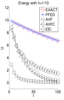
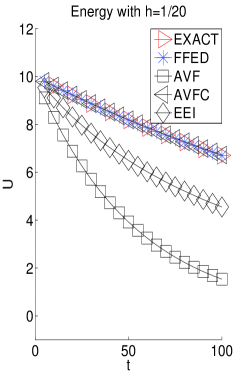
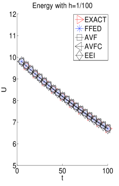
Figure 1: The results of the energy $U$ against the time $t$.

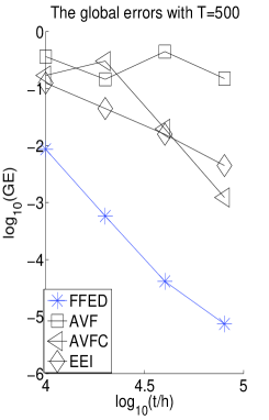
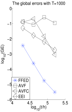
Figure 2: The logarithm of the global errors against the logarithm of $t/h$.

7 Conclusions

In this letter we derived a novel kind of functionally fitted energy-diminishing methods for solving gradient systems. The properties of the methods have been analysed. It was shown that the arbitrary-order methods are unconditionally energy-diminishing and achieve damping for stiff gradient systems. We also discussed the implementations of the methods. The remarkable efficiency of the methods was demonstrated by a numerical test in comparison with three existing numerical methods in the literature.

References

• [1] W. Bao, Q. Du, Computing the ground state solution of Bose-Einstein condensates by a normalized gradient flow, SIAM J. Sci. Comput. 25 (2004) 1674-1697.
• [2] J. Barrett, J. Blowey, Finite element approximation of an Allen-Cahn/Cahn-Hilliard system, IMA J. Numer. Anal. 22 (2002) 11-71.
• [3] L. Chen, Phase-field models for microstructure evolution, Annual review of materials research, 32 (2002) 113-140.
• [4] M. Droske, M. Rumpf, A level set formulation for Willmore flow, Interfaces Free Bound, 6 (2004) 361-378.
• [5] X. Feng, A. Prohl, Error analysis of a mixed finite element method for the Cahn-Hilliard equation, Numer. Math. 99 (2004) 47-84.
• [6] E. Hairer, C. Lubich, Energy-diminishing integration of gradient systems, IMA J. Numer. Anal. 34 (2014) 452-461.
• [7] E. Hairer, C. Lubich, G. Wanner, Geometric Numerical Integration: Structure-Preserving Algorithms for Ordinary Differential Equations, 2nd edn. Springer-Verlag, Berlin, Heidelberg, 2006.
• [8] E. Hairer, G. Wanner, Solving Ordinary Differential Equations II. Stiff and Differential-Algebraic Problems, Springer Series in Computational Mathematics 14, 2nd edn. Springer-Verlag, Berlin, Heidelberg, 1996.
• [9] M. Hochbruck, A. Ostermann, J. Schweitzer, Exponential rosenbrock-type methods, SIAM J. Numer. Anal. 47 (2009) 786-803.
• [10] Y.W. Li, X. Wu, Exponential integrators preserving first integrals or Lyapunov functions for conservative or dissipative systems, SIAM J. Sci. Comput. 38 (2016) 1876-1895.
• [11] Y.W. Li, X. Wu, Functionally fitted energy-preserving methods for solving oscillatory nonlinear Hamiltonian systems, SIAM J. Numer. Anal. 54 (2016) 2036-2059.
• [12] C. Li, X. Wu, The boundness of the operator-valued functions for multidimensional nonlinear wave equations with applications, Appl. Math. Lett. 74 (2017) 60-67.
• [13] C. Lubich, A. Ostermann, Runge-Kutta methods for parabolic equations and convolution quadrature, Math. Comp. 60 (1993) 105-131.
• [14] C. Lubich, A. Ostermann, Runge-Kutta time discretization of reaction-diffusion and Navier-Stokes equations: nonsmooth-data error estimates and applications to long-time behaviour, Appl. Numer. Math. 22 (1996) 279-292.
• [15] R. I. Mclachlan, G. R. W. Quispel, N. Robidoux, A unified approach to Hamiltonian systems, Poisson systems, gradient systems, and systems with Lyapunov functions or first integrals, Phys. Rev. Lett. 81 (1998) 2399-2411
• [16] R. I. McLachlan, G. R. W. Quispel, N. Robidoux, Geometric integration using discrete gradient, Philos. Trans. R. Soc. Lond. A 357 (1999) 1021-1045.
• [17] O. Michailovich, Y. Rathi, A. Tannenbaum, Image segmentation using active contours driven by the Bhattacharyya gradient flow, IEEE Trans. Image Process. 16 (2007) 2787-2801.
• [18] F. Otto, The geometry of dissipative evolution equations: the porous medium equation, Comm. Part. Diff. Equa. 26 (2001) 101-174.
• [19] P. Penzler, M. Rumpf, B. Wirth, A phase-field model for compliance shape optimization in nonlinear elasticity, ESAIM Control Optim. Calc. Var. 18 (2012) 229-258.
• [20] R. Strzodka, M. Droske, M. Rumpf, Image registration by a regularized gradient flow. A streaming implementation in DX9 graphics hardware, Computing, 73 (2004) 373-389.
• [21] B. Wang, A. Iserles, X. Wu, Arbitrary–order trigonometric Fourier collocation methods for multi-frequency oscillatory systems, Found. Comput. Math. 16 (2016) 151-181.
• [22] B. Wang, X. Wu, Arbitrary-order exponential energy-preserving collocation methods for solving conservative or dissipative systems, Preprint, (2017) arXiv:1712.07830
• [23] B. Wang, X. Wu, F. Meng, Trigonometric collocation methods based on Lagrange basis polynomials for multi-frequency oscillatory second-order differential equations, J. Comput. Appl. Math. 313 (2017) 185-201.
• [24] B. Wang, X. Wu, F. Meng, Y. Fang, Exponential Fourier collocation methods for solving first-order differential equations, J. Comput. Math. 35 (2017) 711-736.
• [25] X. Wu, X. You, B. Wang, Structure-Preserving Algorithms for Oscillatory Differential Equations, Springer-Verlag, Berlin, Heidelberg, 2013.