Small-amplitude static periodic patterns at a fluid-ferrofluid interface

Abstract

We establish the existence of static doubly periodic patterns (in particular rolls, rectangles and hexagons) on the free surface of a ferrofluid near onset of the Rosensweig instability, assuming a general (nonlinear) magnetisation law. A novel formulation of the ferrohydrostatic equations in terms of Dirichlet-Neumann operators for nonlinear elliptic boundary-value problems is presented. We demonstrate the analyticity of these operators in suitable function spaces and solve the ferrohydrostatic problem using an analytic version of Crandall-Rabinowitz local bifurcation theory. Criteria are derived for the bifurcations to be sub-, super- or transcritical with respect to a dimensionless physical parameter.

1 Introduction

Consider two static immiscible perfect fluids in the regions

$$\Omega^{\prime} :=\left\{(x,y,z):\,\eta(x,z)<y<d\right\},$$

$$\Omega: =\left\{(x,y,z):\,-d<y<\eta(x,z)\right\}$$

separated by the free surface $\{y=\eta(x,z)\}$, where gravity acts in the negative $y$ direction. The upper fluid is non-magnetisable, while the lower is a ferrofluid with a general nonlinear magnetisation law

$${\mathbf{M}}=\mathbf{M}(\mathbf{H})=m(|\mathbf{H}|)\frac{\mathbf{H}}{|\mathbf{H}|}$$

expressing the relationship between the magnetisation ${\mathbf{M}}$ of the ferrofluid and the strength of the magnetic field ${\mathbf{H}}$. Subjecting the fluids to a vertically directed magnetic field of sufficient strength leads to the emergence of interfacial patterns (see Figure 1).

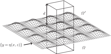
Figure 1: A rectangular periodic pattern at the interface $\left\{y=\eta(x,z)\right\}$.

In this article we present an existence theory for small amplitude, doubly periodic patterns with

$$\eta(\mathbf{x}+\mathbf{l})=\eta(\mathbf{x})$$

for every $\mathbf{l}\in\mathscr{L},$ where $\mathbf{x}=(x,z)$ and $\mathscr{L}$ is the lattice given by

$$\mathscr{L}=\left\{m\mathbf{l}_{1}+n\mathbf{l}_{2}:\ m,n\in\mathbb{Z}\right\}$$

with $\left|\mathbf{l}_{1}\right|=\left|\mathbf{l}_{2}\right|.$ We are especially interested in three patterns which are observed in experiments (Figure 2), namely rolls, rectangles and hexagons (see Figure 3).

1. For rolls we seek functions that are independent of the $z$-direction and choose $\mathbf{l}=(\frac{2\pi}{\omega},0)$, so that the periodic base cell is given by $\left\{x:|x|<\frac{\pi}{\omega}\right\}$.

2. For rectangles we choose $\mathbf{l}_{1}=(\frac{2\pi}{\omega},0)$, $\mathbf{l}_{2}=(0,\frac{2\pi}{\omega})$, so that the periodic base cell is given by $\left\{(x,z):\left|x\right|,\>\left|z\right|<\frac{\pi}{\omega}\right\}$.

3. For hexagons we choose $\mathbf{l}_{1}=\frac{2\pi}{\omega}(1,-\frac{1}{\sqrt{3}})$, $\mathbf{l}_{2}=\frac{2\pi}{\omega}(0,\frac{2}{\sqrt{3}}),$ so that we obtain an additional periodic direction $\mathbf{l}_{3}=\mathbf{l}_{1}+\mathbf{l}_{2}=\frac{2\pi}{\omega}(1,\frac{1}{\sqrt{3}})$ and the periodic base cell is given by $\left\{(x,z):\left|x\right|<\frac{2\pi}{\omega},\>\left|x-\sqrt{3}z\right|<\frac{4\pi}{\omega},\left|x+\sqrt{3}z\right|<\frac{4\pi}{\omega}\right\}$.

Notice that each of these patterns exhibits a rotational symmetry: the shape of the free surface is invariant under a rotation of the $(x,z)$-plane through respectively (i) $\frac{\pi}{2}$, (ii) $\frac{\pi}{3}$ and (iii) ${\pi}$.

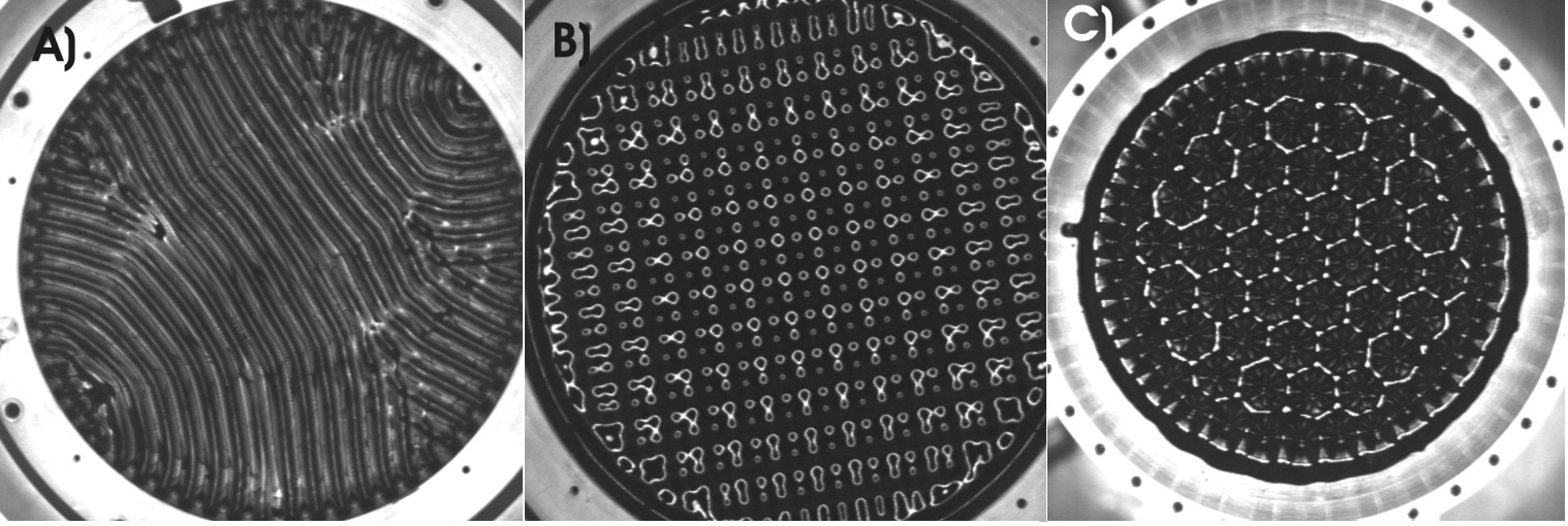
Figure 2: Experimental observation of static patterns at the fluid-ferrofluid interface: A) rolls; B) rectangles; C) hexagons (Fachrichtung Physik, Universität des Saarlandes).

In Section 22.1 we derive the mathematical formulation of this problem from physical principles. The governing equations (equations (10)–(16)) are formulated in terms of perturbations $\phi^{\prime}$ and $\phi$ of magnetic potentials corresponding to a uniform vertically directed magnetic field (of strength $h\mu(h)$ in the upper fluid and $h$ in the lower fluid, where $\mu$ is obtained from the magnetisation law by the formula $\mu(s)=1+m(s)/s$; the potentials are horizontally doubly periodic, satisfying

$$\phi^{\prime}(\mathbf{x}+\mathbf{l},y)=\phi^{\prime}(\mathbf{x},y),\qquad\phi(\mathbf{x}+\mathbf{l},y)=\phi(\mathbf{x},y)$$

for every $\mathbf{l}\in\mathscr{L}$ (with a slight abuse of notation).

This problem was first studied by Cowley and Rosensweig [1]. Using a linear stability analysis, they found that, as the strength $h$ of the magnetic field exceeds a critical value $h_{\mathrm{c}}$, the flat surface destabilises and a hexagonal pattern of peaks appears. This phenomenon is known as the Rosensweig instability. A mathematically rigorous treatment of the problem was given by Twombly and Thomas [2], who used coordinate transformations to ‘flatten’ the free surface by transforming the a priori unknown domains $\Omega^{\prime}$ and $\Omega$ into fixed strips. Applying Lyapunov-Schmidt reduction reduces these transformed equations for rotationally symmetric patterns (see below) to a locally equivalent one-dimensional equation which is solved using the implicit-function theorem; the result is the existence, for values of $h$ near $h_{\mathrm{c}}$, of rolls and rectangles in addition to the hexagonal pattern. Twombly and Thomas’s work is however flawed by some miscalculations and mathematical inconsistencies, and is also restricted to linear magnetisation laws. In this article we present a more systematic approach which is motivated by the corresponding study of doubly periodic travelling water waves by Craig and Nicholls [3]; we also consider general nonlinear magnetisation laws.

We work with dimensionless variables, in terms of which the problem depends upon two dimensionless parameters $\beta$ (whose value $\beta_{0}$ is fixed) and $\gamma$ (see equation (17)), and ‘flatten’ the equations using Dirichlet-Neumann formalism. The Dirichlet-Neumann operator $G^{\prime}$ for the upper fluid domain (given by $\{\eta(x,z)<y<\tfrac{1}{\beta_{0}}\}$ in dimensionless variables) is defined as follows. Fix $\Phi^{\prime}=\Phi^{\prime}(x,z),$ solve the linear boundary-value problem

$$\phi^{\prime}_{xx}+\phi^{\prime}_{yy}+\phi^{\prime}_{zz} =0,\hphantom{\Phi^{\prime}}\quad\qquad\eta<y<\tfrac{1}{\beta_{0}},$$

$$\phi^{\prime} =\Phi^{\prime},\hphantom{0}\quad\qquad y=\eta,$$

$$\phi^{\prime}_{y} =0,\hphantom{\Phi^{\prime}}\quad\qquad y=\tfrac{1}{\beta_{0}},$$

and define

$$G^{\prime}(\eta,\Phi^{\prime}) =-(1+\eta_{x}^{2}+\eta_{z}^{2})^{\frac{1}{2}}\phi^{\prime}_{n}\big{|}_{y=\eta}=-(\phi^{\prime}_{y}-\eta_{x}\phi^{\prime}_{x}-\eta_{z}\phi^{\prime}_{z})\big{|}_{y=\eta}.$$ (1)

The Dirichlet-Neumann operator $G$ for the lower fluid domain $\{-\tfrac{1}{\beta_{0}}<y<\eta(x,z)\}$ is similarly defined as

$$G(\eta,\Phi) =(1+\eta_{x}^{2}+\eta_{z}^{2})^{\frac{1}{2}}\mu(|\operatorname{grad}(\phi+y)|)\phi_{n}\big{|}_{y=\eta}$$

$$=\mu(|\operatorname{grad}(\phi+y)|)(\phi_{y}-\eta_{x}\phi_{x}-\eta_{z}\phi_{z})\big{|}_{y=\eta},$$ (2)

where $\phi$ is the solution of the (in general nonlinear) boundary-value problem

$$\textnormal{div}(\mu(|\operatorname{grad}(\phi+y)|)\operatorname{grad}(\phi+y)) =0,\hphantom{\mu_{1}}\quad\qquad-\tfrac{1}{\beta_{0}}<y<\eta,$$ (3)

$$\phi =\Phi,\hphantom{\mu_{1}}\quad\qquad y=\eta,$$ (4)

$$\mu(|\operatorname{grad}(\phi+y)|)(\phi_{y}+1) =\mu(1),\quad\qquad y=-\tfrac{1}{\beta_{0}}.$$ (5)

The nonlinearity of (3)–(5) is inherited from that of the magnetisation law ${\mathbf{M}}=\mathbf{M}(\mathbf{H})$ (for a linear magnetisation law the value of $\mu$ is constant and (3), (5) are replaced by respectively Laplace’s equation and a linear Neumann boundary condition). In Sections 22.2 and 2.3 we show that $G^{\prime}$ and $G$ are analytic functions of respectively $(\eta,\Phi^{\prime})$ and $(\eta,\Phi)$ in suitable function spaces and use these operators to recast the governing equations in terms of the variables $\Phi^{\prime}=\phi^{\prime}|_{y=\eta}$ and $\Phi=\phi|_{y=\eta}$. The mathematical problem is thus to solve a system of equations of the form

$${\mathcal{G}}(\gamma,(\eta,\Phi^{\prime},\Phi))=0,$$

where ${\mathcal{G}}:{\mathbb{R}}\times X_{0}\rightarrow Y_{0}$ is given explicitly by the left-hand sides of equations (27)–(29) and the function spaces $X_{0}$, $Y_{0}$ are specified in equation (30). Observe that this problem exhibits rotational symmetry: it is invariant under rotations through respectively $\pi$, $\frac{\pi}{2}$ and $\frac{\pi}{3}$ for rolls, rectangles and hexagons, and one may therefore replace $X_{0}$ and $Y_{0}$ by their subspaces of functions that are invariant under these rotations (denoted by $X_{\mathrm{sym}}$ and $Y_{\mathrm{sym}}$).

In Section 3 we discuss the existence of small-amplitude solutions to (31) within the framework of analytic Crandall-Rabinowitz local bifurcation theory (see Buffoni and Toland[4, Chapter 8]), using $\gamma$ as a bifurcation parameter. According to that theory values $\gamma_{0}$ of $\gamma$ at which non-trivial solutions bifurcate from zero (clearly ${\mathcal{G}}(\gamma,0)=0$ for all values of $\gamma$) necessarily have the property that the kernel of the linear operator $L_{0}:=\mathrm{d}_{2}{\mathcal{G}}[\gamma_{0},0]:X_{0}\rightarrow Y_{0}$ is non-trivial. We show that $\ker L_{0}$ is non-trivial if and only if

$$\gamma_{0}=r(|{\bf k}|):=\left(\mu_{1}(\mu_{1}-1)^{2}\bigg{(}\mu_{1}|\mathbf{k}|\coth\frac{|\mathbf{k}|}{\beta_{0}}+S_{1}|\mathbf{k}|\coth\frac{S_{1}|\mathbf{k}|}{\beta_{0}}\bigg{)}^{\!\!-1}-1\right)|\mathbf{k}|^{2}$$

for some $\mathbf{k}\in\mathscr{L}^{\star}\setminus\left\{\mathbf{0}\right\},$ where $\mu_{1}=\mu(1)$, $\dot{\mu}_{1}=\dot{\mu}(1)$ and $S_{1}=\left(\mu_{1}/(\mu_{1}+\dot{\mu}_{1})\right)^{1/2}$. Choosing$\beta_{0}<\mu_{1}(\mu_{1}-1)^{2}/(\mu_{1}+1)$ and $\omega$ so that

$$\gamma_{0}=\left(\mu_{1}(\mu_{1}-1)^{2}\bigg{(}\mu_{1}\omega\coth\frac{\omega}{\beta_{0}}+S_{1}\omega\coth\frac{S_{1}\omega}{\beta_{0}}\bigg{)}^{\!\!-1}-1\right)\omega^{2}$$

is the unique maximum of the mapping $|\mathbf{k}|\mapsto r(|\mathbf{k}|)$, we find that

$$\ker L_{0}=\langle{\left\{\mathbf{v}\sin(\mathbf{k}\cdot\mathbf{x}),\mathbf{v}\cos(\mathbf{k}\cdot\mathbf{x}):\mathbf{k}\in\mathscr{L}^{\star}\ \mathrm{with}\ |\mathbf{k}|=\omega\right\}}\rangle,$$

where ${\bf v}\in{\mathbb{R}}^{3}$ is given by equation (47) (see the discussion to Figure 4); this value $(\beta_{0},\gamma_{0})$ of $(\beta,\gamma)$ corresponds to the Rosensweig instability. The dimension of $\ker L_{0}$ is therefore determined by the number of vectors in $\mathscr{L}^{\star}$ with length $\omega$; for rolls, rectangles and hexagons we find that $\dim\ker L_{0}$ is respectively $2$, $4$ and $6$ (see Figure 5 and Sattinger [5, Section 2] for a general discussion of this point). Because the kernel of $L_{0}$ is multidimensional, one can not use Crandall-Rabinowitz local bifurcation theory directly. To overcome this problem we replace $X_{0}$ and $Y_{0}$ by $X_{\mathrm{sym}}$ and $Y_{\mathrm{sym}}$, thus restricting to solutions that are invariant under rotations through respectively $\pi$, $\frac{\pi}{2}$ and $\frac{\pi}{3}$ for rolls, rectangles and hexagons. These restrictions ensure that $\dim\ker L_{0}=1$ with $\ker L_{0}=\langle{v_{0}}\rangle,$ where $v_{0}=\mathbf{v}\,e_{1}(x,z)$ and

$$e_{1}(x,z)=\left\{\begin{array}[]{ll}\cos\omega x&\qquad\mbox{(rolls)}\\ \cos\omega x+\cos\omega z&\qquad\mbox{(rectangles)}\\ \cos\omega x+\cos\frac{\omega}{2}\left(x+\sqrt{3}z\right)+\cos\frac{\omega}{2}\left(x-\sqrt{3}z\right)&\qquad\mbox{(hexagons).}\end{array}\right.$$

Verifying the remaining conditions in the analytic Crandall-Rabinowitz local bifurcation theorem yields the following result.

Theorem 1.1.

The point $(\gamma_{0},0)$ is a local bifurcation point for (31), that is there exist $\varepsilon>0,$ open neighbourhoods $W_{\mathrm{sym}}$ of $(\gamma_{0},0)$ in $\mathbb{R}\times X_{\mathrm{sym}}$ and $V_{\mathrm{sym}}$ of $0$ in $X_{\mathrm{sym}}$ and analytic functions $w:(-\varepsilon,\varepsilon)\rightarrow V_{\mathrm{sym}}$, $\gamma:(-\varepsilon,\varepsilon)\rightarrow\mathbb{R}$ with $\gamma(0)=\gamma_{0},w(0)=v_{0}$ such that ${\mathcal{G}}(\gamma(s),sw(s))=0$ for every $s\in(-\varepsilon,\varepsilon).$ Furthermore

$$W_{\mathrm{sym}}\cap N=\left\{(\gamma(s),sw(s)):\ 0<|s|<\varepsilon\right\},$$

where

$$N=\left\{(\gamma,v)\in\mathbb{R}\times(V_{\mathrm{sym}}\setminus\left\{0\right\}):{\mathcal{G}}(\gamma,v)=0\right\}.$$

In Section 4 we examine the bifurcating branches identified in Theorem 1.1.

Theorem 1.2.

Branches of small-amplitude doubly periodic solutions to the ferrohydrostatic problem bifurcate from the trivial solution at $\gamma=\gamma_{0}$. The bifurcation is

1. transcritical in the case of hexagons,

2. super- or subcritical in the case of rolls and rectangles, depending upon the sign of a coefficient $\gamma_{2}$ which is determined by $\mu$ and $\omega/\beta_{0}$.

Explicit formulae for the coefficient $\gamma_{2}$ are given in some special cases in Section 4 (such formulae are unwieldy, and it appears in general more appropriate to calculate them numerically for a specific choice of $\mu$). We note in particular that for constant $\mu$ (corresponding to a linear magnetisation law) and very deep fluids, rolls bifurcate subcritically for $\mu<\mu_{\mathrm{c}}^{1}$ and supercritically for $\mu>\mu_{\mathrm{c}}^{1}$, while rectangles bifurcate subcritically for $\mu<\mu_{\mathrm{c}}^{2}$ and supercritically for $\mu>\mu_{\mathrm{c}}^{2}$, where

$$\mu_{\mathrm{c}}^{1}=\frac{21}{11}+\frac{8}{11}\sqrt{5},\qquad\mu_{\mathrm{c}}^{2}=\frac{115+160\sqrt{2}+8\sqrt{184+11\sqrt{2}}}{141+128\sqrt{2}}.$$

The same values were obtained by Silber and Knobloch [6] in a discussion of normal forms for this bifurcation problem and confirmed by Lloyd, Gollwitzer, Rehberg and Richter [7] as part of a wider numerical and experimental investigation.

Finally, we note that supercritical bifurcation of rolls is associated with (supercritical) bifurcation of spatially localised patterns, whose existence has been established by dynamical-systems arguments by Groves, Lloyd & Stylianou [8].

2 Mathematical formulation

2.1 The physical problem

We consider two static immiscible perfect fluids in the regions

$$\Omega^{\prime}:=\{(x,y,z):\,\eta(x,z)<y<d\},\qquad\Omega:=\{(x,y,z):\,-d<y<\eta(x,z)\}$$

separated by the free interface $\{y=\eta(x,z)\}$. The upper, non-magnetisable fluid has unit relative permeability and density $\rho^{\prime}$, while the lower is a ferrofluid with density $\rho$. The relations between the magnetic fields $\mathbf{H}^{\prime}$, $\mathbf{H}$ and the induction fields $\mathbf{B}^{\prime}$, $\mathbf{B}$ are given by the identities

$$\mu_{0}\mathbf{H}^{\prime}=\mathbf{B}^{\prime},\qquad\qquad\mu_{0}(\mathbf{H}+\mathbf{M}(\mathbf{H}))=\mathbf{B}$$

where $\mu_{0}$ is the vacuum permeability and $\mathbf{M}$ is the magnetic intensity of the ferrofluid. (Here, and in the remainder of this paper, equations for ‘primed’ and ‘non-primed’ quantities are supposed to hold in respectively $\Omega^{\prime}$ and $\Omega$.) We suppose that

$$\mathbf{M}(\mathbf{H})=m(|\mathbf{H}|)\frac{\mathbf{H}}{|\mathbf{H}|},$$

where $m$ is a nonnegative function, so that in particular $\mathbf{M}$ and $\mathbf{H}$ are collinear. According to Maxwell’s equations the magnetic and induction fields are respectively irrotational and solenoidal, and introducing magnetic potential functions $\phi^{\prime},\phi$ with

$$-\operatorname{grad}\phi^{\prime}=\mathbf{H}^{\prime},\qquad\qquad-\operatorname{grad}\phi=\mathbf{H},$$

one finds that these potentials satisfy the equations

$$\operatorname{div}(\operatorname{grad}\phi^{\prime})=0,\qquad\qquad\operatorname{div}(\mu(|\operatorname{grad}\,\phi|)\operatorname{grad}\,\phi)=0,$$ (6)

in which

$$\mu(s)=1+\frac{m(s)}{s};$$

we assume that $\mu:(0,\infty)\to\mathbb{R}$ is analytic and satisfies $\mu(1)+\dot{\mu}(1)>0$ (so that the linearised version of the equation for $\phi$ is elliptic). Observe that $\phi^{\prime}$ is harmonic while $\phi$ satisfies a nonlinear elliptic partial differential equation; this nonlinearity is inherited from that of the magnetisation law ${\mathbf{M}}=\mathbf{M}(\mathbf{H})$ (for a linear magnetisation law the value of $\mu$ is constant and the equation for $\phi$ reduces to Laplace’s equation). At the interface we have the magnetic conditions

$$\mathbf{H}^{\prime}\cdot\mathbf{t}_{1}=\mathbf{H}\cdot\mathbf{t}_{1},\qquad\qquad\mathbf{H}^{\prime}\cdot\mathbf{t}_{2}=\mathbf{H}\cdot\mathbf{t}_{2},\qquad\qquad\mathbf{B}^{\prime}\cdot\mathbf{n}=\mathbf{B}\cdot\mathbf{n},$$

where

$$\mathbf{t}_{1} =\cfrac{(1,\eta_{{x}},0)^{\mathrm{T}}}{\sqrt{1+\eta^{2}_{x}}},\qquad\qquad\mathbf{t}_{2}=\cfrac{(0,\eta_{{z}},1)^{\mathrm{T}}}{\sqrt{1+\eta^{2}_{z}}},\qquad\qquad\mathbf{n}=\cfrac{(-\eta_{{x}},1,-\eta_{{z}})^{\mathrm{T}}}{\sqrt{1+\eta^{2}_{x}+\eta^{2}_{z}}}$$

are the tangent and normal vectors to the interface; it follows that

$$\phi^{\prime}-\phi\big{|}_{y=\eta}=0,\qquad\qquad\phi^{\prime}_{n}-\mu(|\operatorname{grad}\,\phi|)\phi_{n}\big{|}_{y=\eta}=0.$$ (7)

The ferrohydrostatic Euler equations are given by

$$-\operatorname{grad}{(p^{\prime}_{0}+\rho^{\prime}gy)}=\mathbf{0},\qquad\qquad\mu_{0}\left({\mathbf{M}(\mathbf{H})\cdot(\partial_{x},\partial_{z},\partial_{y})^{\mathrm{T}}}\right){\mathbf{H}}-\operatorname{grad}({p^{\star}+\rho gy})=\mathbf{0}$$

(Rosensweig [9, Section 5.1]), in which $g$ is the acceleration due to gravity, $p^{\prime}_{0}$ is the pressure in the upper fluid and $p^{\star}$ is a composite of the magnetostrictive and fluid-magnetic pressures. The calculation

$$\left(\mathbf{M}(\mathbf{H})\cdot(\partial_{x},\partial_{y},\partial_{z})^{\mathrm{T}}\right){\mathbf{H}}=m(|{\mathbf{H}}|)\,\operatorname{grad}\,|{\mathbf{H}}|=\operatorname{grad}\left(\int_{0}^{|\mathbf{H}|}m(t)\,\mathrm{d}t\right)$$

shows that these equations are equivalent to

$$-(p^{\prime}_{0}+\rho^{\prime}gy)=C^{\prime}_{0},\qquad\qquad\mu_{0}\int_{0}^{|\mathbf{H}|}m(t)\,\mathrm{d}t-(p^{\star}+\rho gy)=C_{0},$$ (8)

where $C^{\prime}_{0},C_{0}$ are constants. The ferrohydrostatic boundary condition is given by

$$p^{\star}+\frac{\mu_{0}}{2}({\mathbf{M}(\mathbf{H})\cdot\mathbf{n}})^{2}=p^{\prime}_{0}+2\kappa\sigma$$

for $y=\eta(x,z)$ (Rosensweig [9, Section 5.2]), in which $\sigma>0$ is the coefficient of surface tension and

$$2\kappa =-\cfrac{\eta_{{xx}}(1+\eta_{{z}}^{2})+\eta_{{zz}}(1+\eta_{{x}}^{2})-2\eta_{{x}}\eta_{{z}}\eta_{{xz}}}{(1+\eta_{{x}}^{2}+\eta_{{z}}^{2})^{3/2}}$$

is the mean curvature of the interface. Using (8), we find that

$$\dfrac{\mu_{0}}{2}(\mathbf{M}(\mathbf{H})\cdot\mathbf{n})^{2}+{\mu_{0}}\int_{0}^{|\mathbf{H}|}m(t)\,\mathrm{d}t+C+({\rho^{\prime}-\rho})g\eta-2\sigma\kappa =0,$$

where $C=C^{\prime}_{0}-C_{0},$ or equivalently

$$C+\mu_{0}\sqrt{1+\eta_{x}^{2}+\eta_{z}^{2}}(\phi^{\prime}_{y}\phi^{\prime}_{n}-\mu(|\operatorname{grad}\,\phi|)\phi_{y}\phi_{n})$$

$$\qquad\mbox{}-({\rho-\rho^{\prime}})g\eta-2\sigma\kappa-\mu_{0}\left(\frac{1}{2}{|{\operatorname{grad}\,\phi^{\prime}}|^{2}-M(|{\operatorname{grad}\,\phi}|)}\right)=0$$ (9)

for $y=\eta(x,z)$ with

$$M(s)=\int_{0}^{s}t\mu(t)\,\mathrm{d}t.$$

The requirement that a uniform magnetic field and flat interface solves the physical problem, that is $(\eta_{0},\phi^{\prime}_{0},\phi_{0})=(0,\mu(h)hy,hy)$ is a solution to (6), (7) and (9), leads us to choose$C=-\mu_{0}M(h)-\mu_{0}\mu(h)(\mu(h)-1)h^{2}/2$; we write $(\tilde{\eta},\tilde{\phi}^{\prime},\tilde{\phi})=(\eta,\phi^{\prime},\phi)+(\eta_{0},\phi^{\prime}_{0},\phi_{0})$ (so that $(\tilde{\eta},\tilde{\phi}^{\prime},\tilde{\phi})=(0,0,0)$ is the ‘trivial’ solution) and drop the tildes for notational simplicity.

The next step is to introduce dimensionless variables

$$(\hat{x},\hat{y},\hat{z})=\frac{\mu_{0}h^{2}}{\sigma}(x,y,z),\quad\hat{\eta}:=\frac{\mu_{0}h^{2}}{\sigma}\eta,\quad\hat{\phi}^{\prime}:=\frac{\mu_{0}h}{\sigma}\phi^{\prime},\quad\hat{\phi}:=\frac{\mu_{0}h}{\sigma}\phi$$

and functions

$$\hat{\mu}(s):=\mu(hs),\qquad\hat{M}(s):=M(hs).$$

We find that

$$\phi^{\prime}_{xx}+\phi^{\prime}_{yy}+\phi^{\prime}_{zz} =0,\qquad\qquad\eta(x,z)<y<\tfrac{1}{\beta_{0}},$$ (10)

$$\operatorname{div}(\mu(|\operatorname{grad}(\phi+y)|)\operatorname{grad}(\phi+y)) =0,\qquad\qquad-\tfrac{1}{\beta_{0}}<y<\eta(x,z),$$ (11)

with boundary conditions

$$\phi^{\prime}_{y} =0,\qquad\qquad y=\tfrac{1}{\beta_{0}},$$ (12)

$$\mu(|\operatorname{grad}(\phi+y)|)(\phi_{y}+1)-\mu(1) =0,\qquad\qquad y=-\tfrac{1}{\beta_{0}},$$ (13)

$$\phi^{\prime}-\phi+\left({\mu(1)-1}\right)\eta =0,\qquad\qquad y=\eta(x,z),$$ (14)

$$(\phi^{\prime}+\mu(1)y)_{n}-\mu(|\operatorname{grad}(\phi+y)|)(\phi+y)_{n} =0,\qquad\qquad y=\eta(x,z),$$ (15)

and

$$-M(1)-\mu(1)\left(\frac{1}{2}\mu(1)-1\right)-\gamma\eta-2\sigma\kappa$$

$$\quad\mbox{}-\frac{1}{2}{|{\operatorname{grad}(\phi^{\prime}+\mu(1)y)}|^{2}+M(|{\operatorname{grad}(\phi+y)}|)}$$

$$\quad\mbox{}{+\sqrt{1+\eta_{x}^{2}+\eta_{z}^{2}}({\phi^{\prime}_{y}+\mu(1)})(\phi^{\prime}+\mu(1)y)_{n}}$$

$$\quad\mbox{}{-\sqrt{1+\eta_{x}^{2}+\eta_{z}^{2}}\mu(|\operatorname{grad}(\phi+y)|)({\phi_{y}+1})(\phi+y)_{n}}=0,\qquad\qquad y=\eta(x,z),$$ (16)

where

$$\alpha=\frac{(\rho-\rho^{\prime})gd}{\mu_{0}h^{2}},\qquad\beta=\frac{\sigma}{\mu_{0}h^{2}d},\qquad\gamma=\alpha\beta$$ (17)

and the hats have been dropped for notational simplicity.

We seek periodic solutions to (10)–(16) satisfying

$$\eta(\mathbf{x}+\mathbf{l})=\eta(\mathbf{x}),\qquad\phi^{\prime}(\mathbf{x}+\mathbf{l},y)=\phi^{\prime}(\mathbf{x},y),\qquad\phi(\mathbf{x}+\mathbf{l},y)=\phi(\mathbf{x},y)$$

for every $\mathbf{l}\in\mathscr{L}$ (with a slight abuse of notation), where $\mathbf{x}=(x,z)$ and $\mathscr{L}$ is the lattice given by

$$\mathscr{L}=\left\{m\mathbf{l}_{1}+n\mathbf{l}_{2}:\ m,n\in\mathbb{Z}\right\}$$

with $\left|{\mathbf{l}_{1}}\right|=\left|{\mathbf{l}_{2}}\right|.$ Choose $\mathbf{k}_{1},\mathbf{k}_{2}$ with $\mathbf{k}_{i}\cdot\mathbf{l}_{j}=2\pi\delta_{ij}$ for $i,j=1,2$ and define the dual lattice $\mathscr{L}^{\star}$ to $\mathscr{L}$ by

$$\mathscr{L}^{\star}=\left\{{m\mathbf{k}_{1}+n\mathbf{k}_{2}:\ m,n\in\mathbb{Z}}\right\},$$

so that our periodic functions can be written as

$$\eta(\mathbf{x})=\sum_{\mathbf{k}\in\mathscr{L}^{\star}}\eta_{{}_{\mathbf{k}}}\mathrm{e}^{\mathrm{i}\mathbf{k}\cdot\mathbf{x}},\qquad\phi^{\prime}(\mathbf{x},y)=\sum_{\mathbf{k}\in\mathscr{L}^{\star}}\phi^{\prime}_{{}_{\mathbf{k}}}(y)\mathrm{e}^{\mathrm{i}\mathbf{k}\cdot\mathbf{x}},\qquad\phi(\mathbf{x},y)=\sum_{\mathbf{k}\in\mathscr{L}^{\star}}\phi_{{}_{\mathbf{k}}}(y)\mathrm{e}^{\mathrm{i}\mathbf{k}\cdot\mathbf{x}},$$

where $\eta_{{}_{-\mathbf{k}}}=\bar{\eta}_{{}_{\mathbf{k}}},\phi^{\prime}_{{}_{-\mathbf{k}}}=\bar{\phi^{\prime}}_{{}_{\mathbf{k}}},\phi_{{}_{-\mathbf{k}}}=\bar{\phi}_{{}_{\mathbf{k}}}$. We are especially interested in three periodic patterns, namely rolls, rectangles and hexagons (see Figure 3).

1. For rolls we seek functions that are independent of the $z$-direction and we choose$\mathbf{l}=(\frac{2\pi}{\omega},0),$ so that the dual lattice $\mathscr{L}^{\star}$ is generated by $\mathbf{k}=(\omega,0)$ and the periodic base cell is given by

   $$\left\{x:|x|<\frac{\pi}{\omega}\right\}.$$

   Furthermore, the $z$-independent versions of equations (10)–(16) are invariant under the reflection $x\mapsto-x$ (which corresponds to a rotation through ${\pi}$ in the $(x,z)$-plane).

2. For rectangles we choose $\mathbf{l}_{1}=(\frac{2\pi}{\omega},0)$ and $\mathbf{l}_{2}=(0,\frac{2\pi}{\omega})$, so that the dual lattice $\mathscr{L}^{\star}$ is generated by $\mathbf{k}_{1}=({\omega},0)$ and $\mathbf{k}_{2}=(0,{\omega})$ and the periodic base cell is given by

   $$\left\{(x,z):|x|,\>|z|<\frac{\pi}{\omega}\right\}.$$

   Furthermore, equations (10)–(16) are invariant under rotations through $\pi/2$ in the $(x,z)$-plane.

3. For hexagons we choose $\mathbf{l}_{1}=\frac{2\pi}{\omega}(1,-\frac{1}{\sqrt{3}})$ and $\mathbf{l}_{2}=\frac{2\pi}{\omega}(0,\frac{2}{\sqrt{3}}),$ so that we obtain an additional periodic direction $\mathbf{l}_{3}=\mathbf{l}_{1}+\mathbf{l}_{2}=\frac{2\pi}{\omega}(1,\frac{1}{\sqrt{3}})$. The dual lattice $\mathscr{L}^{\star}$ is generated by $\mathbf{k}_{1}=(\omega,0)$ and $\mathbf{k}_{2}=\omega(\frac{1}{2},\frac{\sqrt{3}}{2})$ and the periodic base cell is given by

   $$\left\{(x,z):|x|<\frac{2\pi}{\omega},\>\left|{x-\sqrt{3}z}\right|<\frac{4\pi}{\omega}\mbox{ and }\left|{x+\sqrt{3}z}\right|<\frac{4\pi}{\omega}\right\}.$$

   Furthermore, equations (10)–(16) are invariant under rotations through ${\pi}/{3}$ in the $(x,z)$-plane.

The mathematical problem is thus to solve (10)–(16) for periodic functions $\eta,\phi^{\prime}$ and $\phi$ in the domains $\Gamma$, $\Omega_{\mathrm{per}}^{\prime}$ and $\Omega_{\mathrm{per}},$ where

$$\Omega_{\mathrm{per}}^{\prime}:=\left\{(x,y,z):(x,z)\in\Gamma\right\}\cap\Omega^{\prime},\qquad\Omega_{\mathrm{per}}:=\left\{(x,y,z):(x,z)\in\Gamma\right\}\cap\Omega$$

and $\Gamma$ is the parallelogram defined by $\mathbf{l}_{1}$ and $\mathbf{l}_{2}$ (or by $\mathbf{l}$ in the case of rolls).

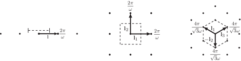
Figure 3: The lattice $\mathscr{L}$ and periodic base cell for rolls (left), rectangles (centre) and hexagons (right).

2.2 Dirichlet-Neumann formalism

The Dirichlet-Neumann operator $G^{\prime}$ for the upper fluid domain $\{\eta(x,z)<y<\tfrac{1}{\beta_{0}}\}$ is defined as follows. Fix $\Phi^{\prime}=\Phi^{\prime}(x,z),$ solve the linear boundary-value problem

$$\phi^{\prime}_{xx}+\phi^{\prime}_{yy}+\phi^{\prime}_{zz} =0,\hphantom{\Phi^{\prime}}\quad\qquad\eta<y<\tfrac{1}{\beta_{0}},$$ (18)

$$\phi^{\prime} =\Phi^{\prime},\hphantom{0}\quad\qquad y=\eta,$$ (19)

$$\phi^{\prime}_{y} =0,\hphantom{\Phi^{\prime}}\quad\qquad y=\tfrac{1}{\beta_{0}}.$$ (20)

and define

$$G^{\prime}(\eta,\Phi^{\prime}) =-(1+\eta_{x}^{2}+\eta_{z}^{2})^{\frac{1}{2}}\phi^{\prime}_{n}\big{|}_{y=\eta}=-(\phi^{\prime}_{y}-\eta_{x}\phi^{\prime}_{x}-\eta_{z}\phi^{\prime}_{z})\big{|}_{y=\eta}.$$ (21)

The Dirichlet-Neumann operator $G$ for the lower fluid domain $\{-\tfrac{1}{\beta_{0}}<y<\eta(x,z)\}$ is similarly defined as

$$G(\eta,\Phi) =(1+\eta_{x}^{2}+\eta_{z}^{2})^{\frac{1}{2}}\mu(|\operatorname{grad}(\phi+y)|)\phi_{n}\big{|}_{y=\eta}$$

$$=\mu(|\operatorname{grad}(\phi+y)|)(\phi_{y}-\eta_{x}\phi_{x}-\eta_{z}\phi_{z})\big{|}_{y=\eta},$$ (22)

where $\phi$ is the solution of the (in general nonlinear) boundary-value problem

$$\textnormal{div}(\mu(|\operatorname{grad}(\phi+y)|)\operatorname{grad}(\phi+y)) =0,\hphantom{\mu_{1}}\quad\qquad-\tfrac{1}{\beta_{0}}<y<\eta,$$ (23)

$$\phi =\Phi,\hphantom{\mu_{1}}\quad\qquad y=\eta,$$ (24)

$$\mu(|\operatorname{grad}(\phi+y)|)(\phi_{y}+1) =\mu(1),\quad\qquad y=-\tfrac{1}{\beta_{0}}.$$ (25)

It is also convenient to introduce auxiliary operators $H^{\prime}$ and $H$ given by

$$H^{\prime}(\eta,\Phi^{\prime})=\phi^{\prime}_{y}|_{y=\eta},\qquad H(\eta,\Phi)=\phi_{y}|_{y=\eta},$$ (26)

where $\phi^{\prime}$ and $\phi$ are the solutions to the boundary-value problems (18)–(20) and (23)–(25). Using this Dirichlet-Neumann formalism, we can recast the governing equations (10)–(16) in terms of the variables $\eta$, $\Phi^{\prime}=\phi^{\prime}|_{y=\eta}$ and $\Phi=\phi|_{y=\eta}$ as

$$\Phi^{\prime}-\Phi+(\mu(1)-1)\eta =0,$$ (27)

$$G^{\prime}(\eta,\Phi^{\prime})+G(\eta,\Phi)+(\mu^{\star}-\mu(1)) =0$$ (28)

and

$$-\gamma\eta+\nabla\cdot\left({\cfrac{\nabla\eta}{\sqrt{1+|{\nabla{\eta}}|^{2}}}}\right)+\frac{1}{2}\left({1+\left|{\nabla\eta}\right|^{2}}\right)H^{\prime}(\eta,\Phi^{\prime})^{2}-\frac{1}{2}|{\nabla\Phi^{\prime}}|^{2}\Big{|}_{y=\eta}$$

$$\qquad\mbox{}-\mu(1)G^{\prime}(\eta,\Phi^{\prime})-G(\eta,\Phi)-(\mu^{\star}-\mu(1))$$

$$\qquad\mbox{}+(M^{\star}-M(1))-\mu^{\star}H(\eta,\Phi)-H(\eta,\Phi)G(\eta,\Phi)=0,$$ (29)

in which $\nabla=(\partial_{x},\partial_{z})^{\mathrm{T}},$ $M(s)=\displaystyle\int_{0}^{s}t\mu(t)\,\mathrm{d}t$,

$$\mu^{\star} =\mu\!\left(\!\left({|\nabla\Phi|^{2}+2(1-\nabla\eta\cdot\nabla\Phi)H(\eta,\Phi)+(1+|\nabla\eta|^{2})H(\eta,\Phi)^{2}+1}\right)^{{1}/{2}}\right),$$

$$M^{\star} =M\!\left(\!\left({|\nabla\Phi|^{2}+2(1-\nabla\eta\cdot\nabla\Phi)H(\eta,\Phi)+(1+|\nabla\eta|^{2})H(\eta,\Phi)^{2}+1}\right)^{{1}/{2}}\right).$$

We study equations (27)–(29) in the standard Sobolev spaces

$$H_{\mathrm{per}}^{r}(\Gamma)=\left\{\zeta=\sum_{\mathbf{k}\in\mathscr{L}^{\star}}\zeta_{{}_{\mathbf{k}}}\mathrm{e}^{\mathrm{i}\mathbf{k}\cdot\mathbf{x}}:\zeta_{-\mathbf{k}}=\overline{\zeta_{\mathbf{k}}},\,\left\lVert\zeta\right\rVert_{r}<\infty\right\},\qquad\left\lVert\zeta\right\rVert_{r}^{2}:=C(\Gamma)\!\!\sum_{\mathbf{k}\in\mathscr{L}^{\star}}\left(1+|\mathbf{k}|^{2}\right)^{r}|\zeta_{{}_{\mathbf{k}}}|^{2},$$

where $\mathscr{L}^{\star}$ is the dual lattice to $\mathscr{L}$, and their subspaces

$$\bar{H}_{\mathrm{per}}^{r}(\Gamma) =\left\{\zeta\in H^{r}_{\mathrm{\mathrm{per}}}(\Gamma):\zeta_{{}_{\mathbf{0}}}=0\right\}$$

consisting of functions with zero mean (the value of the normalisation constant $C(\Gamma)$ is $2\pi/\omega$ for rolls, $4(\pi/\omega)^{2}$ for rectangles and $8/\sqrt{3}(\pi/\omega)^{2}$ for hexagons). In Section 22.3 below we establish the following theorem. (A function is ‘analytic at the origin’ if is defined and analytic in a neighbourhood of the origin; in particular it has a convergent Maclaurin series.)

Theorem 2.1.

Suppose that $s>5/2$. Formulae (21), (22) and (26) define mappings $G^{\prime}$, $G:H^{s}_{\mathrm{per}}(\Gamma)\times H^{s-1/2}_{\mathrm{per}}(\Gamma)\rightarrow H^{s-3/2}_{\mathrm{per}}(\Gamma)$ and $H^{\prime}$, $H:H^{s}_{\mathrm{per}}(\Gamma)\times H^{s-1/2}_{\mathrm{per}}(\Gamma)\rightarrow H^{s-3/2}_{\mathrm{per}}(\Gamma)$ which are analytic at the origin.

Define

$$X_{0}:=H^{s+1/2}_{\mathrm{per}}(\Gamma)\times\bar{H}^{s}_{\mathrm{per}}(\Gamma)\times H^{s}_{\mathrm{per}}(\Gamma),\qquad Y_{0}:=H^{s}_{\mathrm{per}}(\Gamma)\times\bar{H}^{s-1}_{\mathrm{per}}(\Gamma)\times H^{s-3/2}_{\mathrm{per}}(\Gamma)$$ (30)

for $s>5/2$. Using Theorem 2.1 and the fact that $H^{r}(\Gamma)$ is a Banach algebra for $r>1$, we find that the left-hand sides of equations (27)–(29) define a function ${\mathcal{G}}:\mathbb{R}\times X_{0}\to Y_{0}$ which is analytic at the origin. (A straightforward calculation shows that

$$\int_{\Gamma}\left(G^{\prime}(\eta,\Phi^{\prime})+G(\eta,\Phi)+(\mu^{\star}-\mu(1))\right)=0$$

and explains the choice of functions with zero mean in the second component of $Y_{0}$; using functions with zero mean in the second component of $X_{0}$ on the other hand ensures that the kernel of the linear operator $\mathrm{d}_{2}{\mathcal{G}}[\gamma,0]$ does not contain any constant terms for any $\gamma\in\mathbb{R}$). The mathematical problem is thus to solve

$${\mathcal{G}}(\gamma,(\eta,\Phi^{\prime},\Phi))=0,$$ (31)

for $(\gamma,(\eta,\Phi^{\prime},\Phi))\in{\mathbb{R}}\times V_{0}$, where $V_{0}$ is a neighbourhood of the origin in $X_{0}$ and ${\mathcal{G}}(\gamma,0)=0$ for all $\gamma\in\mathbb{R}.$ Observe that this problem exhibits rotational symmetry: it is invariant under rotations through respectively $\pi$, $\frac{\pi}{2}$ and $\frac{\pi}{3}$ for rolls, rectangles and hexagons, and one may therefore replace $X_{0}$ and $Y_{0}$ by their subspaces of functions that are invariant under these rotations (denoted by $X_{\mathrm{sym}}$ and $Y_{\mathrm{sym}}$).

2.3 Analyticity of the Dirichlet-Neumann operators

We study the boundary-value problems (23)–(25) and (18)–(20) by transforming them into equivalent problems in fixed domains (cf. Nicholls and Reitich [10] and Twombly and Thomas [2]). The change of variable

$$\tilde{y}=\cfrac{y-\eta}{1+\beta_{0}\eta},\qquad u(x,\tilde{y},z)=\phi(x,y,z)$$ (32)

transforms the variable domain $\Omega_{\mathrm{per}}$ into the fixed domain $\Sigma=\left\{{(x,y,z):(x,z)\in\Gamma,y\in(-\tfrac{1}{\beta_{0}},0)}\right\}$ and the boundary-value problem (23)–(25) into

$$\textnormal{div}\big{(}\mu^{\dagger}(\operatorname{grad}(u+y)-(F_{1}(\eta,u),F_{3}(\eta,u),F_{2}(\eta,u))^{\mathrm{T}})\big{)} =0, -\tfrac{1}{\beta_{0}}<y<0,$$ (33)

$$u-\Phi =0, y=0,$$ (34)

$$\mu^{\dagger}\big{(}\operatorname{grad}(u+y).(0,1,0)^{\mathrm{T}}-F_{3}(\eta,u)\big{)}-\mu(1) =0, y=-\tfrac{1}{\beta_{0}},$$ (35)

where

$$F_{1}(\eta,u)=-\eta u_{x}+(1+\beta_{0}y)\eta_{x}u_{y},\qquad F_{2}(\eta,u)=-\eta u_{z}+(1+\beta_{0}y)\eta_{z}u_{y},$$

$$F_{3}(\eta,u)=\frac{\beta_{0}\eta u_{y}}{1+\beta_{0}\eta}+(1+\beta_{0}y)(\eta_{x}u_{x}+\eta_{z}u_{z})-\frac{(1+\beta_{0}y)^{2}}{1+\beta_{0}\eta}(\eta^{2}_{x}+\eta^{2}_{z})u_{y}$$

and

$$\mu^{\dagger}=\mu\left(\left|\frac{1}{1+\beta_{0}\eta}\big{(}\operatorname{grad}u-(F_{1}(\eta,u),0,F_{2}(\eta,u))^{\mathrm{T}}\big{)}+(0,1,0)^{\mathrm{T}}\right|\right)$$

(we have again dropped the tildes for notational simplicity).

Theorem 2.2.

Suppose that $s>5/2.$ There exist open neighbourhoods $V$ and $U$ of the origin in respectively $H_{\mathrm{per}}^{s}(\Gamma)\times H_{\mathrm{per}}^{s-1/2}(\Gamma)$ and $H_{\mathrm{per}}^{s}(\Sigma)$ such that the boundary-value problem (33)–(35) has a unique solution $u=u(\eta,\Phi)$ in $U$ for each $(\eta,\Phi)\in V$. Furthermore $u(\eta,\Phi)$ depends analytically upon $\eta$ and $\Phi$.

Proof.

Write the left-hand sides of equations (33)–(35) as

$${\mathcal{H}}(u,\eta,\Phi)=0,$$

and observe that ${\mathcal{H}}:H_{\mathrm{per}}^{s}(\Sigma)\times H_{\mathrm{per}}^{s}(\Gamma)\times H_{\mathrm{per}}^{s-1/2}(\Gamma)$ is analytic at the origin with

$${\mathcal{H}}(0,0,0)=0.$$

Furthermore, the calculation

$$\mathrm{d}_{1}{\mathcal{H}}[0,0,0](u)=\begin{pmatrix}\mu_{1}(u_{xx}+S_{1}^{-2}u_{yy}+u_{zz})\\ u|_{y=0}\\ \mu_{1}S_{1}^{-2}u_{y}|_{y=-\frac{1}{\beta_{0}}}\end{pmatrix},$$

where $\mu_{1}=\mu(1)$, $\dot{\mu}_{1}=\dot{\mu}(1)$ and $S_{1}=\left(\mu_{1}/(\mu_{1}+\dot{\mu}_{1})\right)^{1/2}$, and standard existence and regularity theory for elliptic linear boundary-value problems show that $\mathrm{d}_{1}{\mathcal{H}}[0,0,0]:H_{\mathrm{per}}^{s}(\Sigma)\rightarrow H_{\mathrm{per}}^{s-2}\times H_{\mathrm{per}}^{s-1/2}\times H_{\mathrm{per}}^{s-3/2}(\Gamma)$ is an isomorphism. The stated result now follows from the analytic implicit-function theorem. ∎

The transformation (32) converts the formulae

$$G(\eta,\Phi)=\mu(|\operatorname{grad}(\phi+y)|)(\phi_{y}-\eta_{x}\phi_{x}-\eta_{z}\phi_{z})\big{|}_{y=\eta},\qquad H(\eta,\Phi)=\phi_{y}\big{|}_{y=\eta}$$

into

$$G(\eta,\Phi)=\mu^{\dagger}(u_{y}-F_{3}(\eta,u))\big{|}_{y=0},\qquad H(\eta,\Phi)=\left.\frac{u_{y}}{1+\beta_{0}\eta}\right|_{y=0},$$ (36)

where $u=u(\eta,\Phi)$ is the unique solution to (33)–(35).

Theorem 2.3.

Suppose that $s>5/2$. The formulae (36) define analytic functions $G$, $H:V\rightarrow H_{\mathrm{per}}^{s-3/2}(\Gamma)$.

To compute the Taylor-series representations of $u$ and $G$ we begin with the function$\nu:(H^{s-1}_{\mathrm{per}}(\Sigma))^{3}\to H^{s-1}_{\mathrm{per}}(\Sigma)$ defined by

$$\nu(T)=\mu(|T+(0,1,0)^{\mathrm{T}}|).$$

Observing that $\nu$ is analytic at the origin, we write its Taylor series as

$$\nu(T)=\sum_{j=0}^{\infty}\nu^{j}(\{T\}^{(j)}),$$ (37)

where $\nu^{j}\in\mathcal{L}^{j}_{\mathrm{s}}((H^{s-1}_{\mathrm{per}}(\Sigma))^{3},H^{s-1}_{\mathrm{per}}(\Sigma))$ is given by

$$\nu^{j}(T_{1},\ldots,T_{j})=\frac{1}{j!}\mathrm{d}^{j}\nu[0](T_{1},\ldots,T_{j})$$

and may be computed explicitly from $\mu$ (note in particular that $\nu^{0}=\mu_{1}$). The functions$u^{n}\in\mathcal{L}^{n}_{\mathrm{s}}(H^{s}_{\mathrm{per}}(\Gamma)\times H^{s-1/2}_{\mathrm{per}}(\Gamma),H^{s}_{\mathrm{per}}(\Sigma))$ (with $u^{0}=0$) in the corresponding series

$$u(\eta,\Phi)=\sum^{\infty}_{n=0}u^{n}\big{(}\{(\eta,\Phi)\}^{(n)}\big{)}$$ (38)

may be computed recursively by substituting the Ansatz (37), (38) into equations (33)–(35). Consistently abbreviating $m^{n}\big{(}\{(\eta,\Phi)\}^{(n)}\big{)}$ to $m^{n}$ for notational simplicity, one finds after a lengthy but straightforward calculation that

$$\operatorname{div}(L\,\operatorname{grad}\,u^{1}) =0, \operatorname{div}(L\,\operatorname{grad}\,u^{n}-F^{n}) =0,\qquad\qquad-\tfrac{1}{\beta_{0}}<y<0,$$

$$u^{1}-\Phi =0, u^{n} =0,\qquad\qquad y=0,$$

$$u^{1}_{y} =0, (L\,\operatorname{grad}\,u^{n}-F^{n})\cdot(0,1,0)^{\mathrm{T}} =0,\qquad\qquad y=-\tfrac{1}{\beta_{0}}$$

for $n\geq 2$, where

$$L =\begin{pmatrix}1&0&0\\ 0&S_{1}^{-2}&0\\ 0&0&1\end{pmatrix},$$

$$\mu_{1}F^{n} =\mu_{1}\!\left(\!(F^{n}_{1},F^{n}_{3},F^{n}_{2})^{\mathrm{T}}\!-\frac{\dot{\mu}_{1}}{\mu_{1}}\sum_{j=1}^{n}\left(-\beta_{0}\eta\right)^{j}u^{n-j}_{y}(0,1,0)^{\mathrm{T}}\!\!\right)$$

$$\qquad\mbox{}-\sum_{j=0}^{n}\nu^{1}(T^{j})(\operatorname{grad}\,u^{n-j}-(F^{n-j}_{1},F^{n-j}_{3},F^{n-j}_{2})^{\mathrm{T}})$$

$$\qquad\mbox{}-R^{n}(0,1,0)^{\mathrm{T}}-\sum_{j=0}^{n}R^{j}(\operatorname{grad}\,u^{n-j}-(F^{n-j}_{1},F^{n-j}_{3},F^{n-j}_{2})^{\mathrm{T}})$$

and

$$F^{n}_{1} =-\beta_{0}\eta u^{n-1}_{x}+(1+\beta_{0}y)\eta_{x}u^{n-1}_{y},\qquad F^{n}_{2}=-\beta_{0}\eta u^{n-1}_{z}+(1+\beta_{0}y)\eta_{z}u^{n-1}_{y},$$

$$F^{n}_{3} =\beta_{0}\eta\sum^{n-1}_{j=0}\left(-\beta_{0}\eta\right)^{j}u^{n-1-j}_{y}+(1+\beta_{0}y)(\eta_{x}u^{n-1}_{x}+\eta_{z}u^{n-1}_{z})$$

$$\qquad\mbox{}-(1+\beta_{0}y)^{2}(\eta^{2}_{x}+\eta^{2}_{z})\sum^{n-2}_{j=0}\left(-\beta_{0}\eta\right)^{j}u^{n-2-j}_{y},$$

$$T^{n} =\sum_{j=0}^{n}\left(-\beta_{0}\eta\right)^{j}\left(\operatorname{grad}\,u^{{n-j}}-(F^{{n-j}}_{1},0,F^{{n-j}}_{2})^{\mathrm{T}}\right),\qquad R^{n}=\sum_{\begin{subarray}{c}2\leq j\leq n,\\ \begin{subarray}{c}h_{1}+\ldots+h_{j}=n\end{subarray}\end{subarray}}\nu^{j}\!(T^{h_{1}},\dots,T^{h_{j}}).$$

The Taylor-series representations of $G$ and $H$ are thus given by

$$G(\eta,\Phi)=\sum^{\infty}_{n=0}G_{n}\big{(}\{(\eta,\Phi)\}^{(n)}\big{)},\qquad H(\eta,\Phi)=\sum^{\infty}_{n=0}H_{n}\big{(}\{(\eta,\Phi)\}^{(n)}\big{)},$$

where

$$G_{n}=\left.\mu_{1}I^{n}+\sum_{j=0}^{n}\nu^{1}(T^{j})I^{n-j}+\sum_{j=0}^{n}R^{j}I^{n-j}\right|_{y=0},\qquad H_{n}=\sum_{j=0}^{n}(-\beta_{0}\eta)^{j}u^{n-j}_{y}\Bigg{|}_{y=0},$$

and

$$I^{n} =\sum_{j=0}^{n}\left(-\beta_{0}\eta\right)^{j}u_{y}^{n-j}+\sum_{j=0}^{n-2}\left(-\beta_{0}\eta\right)^{j}(\eta^{2}_{x}+\eta^{2}_{z})u_{y}^{n-j-2}-(\eta_{x}u^{n-1}_{x}+\eta_{z}u^{n-1}_{z}).$$

For later use we record the formulae

$$G_{1} =\mu_{1}u_{y}^{1}\big{|}_{y=0},$$

$$G_{2} =\mu_{1}\left(\sum_{j=0}^{2}\left(-\beta_{0}\eta\right)^{j}u_{y}^{2-j}-(\eta_{x}u^{1}_{x}+\eta_{z}u^{1}_{z})\right)+\dot{\mu}_{1}(u_{y}^{1})^{2}\Bigg{|}_{y=0},$$

$$G_{3} =\mu_{1}\left(\sum_{j=0}^{3}\left(-\beta_{0}\eta\right)^{j}u_{y}^{3-j}+(\eta^{2}_{x}+\eta^{2}_{z})u_{y}^{1}-(\eta_{x}u^{2}_{x}+\eta_{z}u^{2}_{z})\right)$$

$$\qquad\mbox{}+\dot{\mu}_{1}\left(2\sum_{j=0}^{2}\left(-\beta_{0}\eta\right)^{j}u_{y}^{2-j}-(\eta_{x}u^{1}_{x}+\eta_{z}u^{1}_{z})\right)\!\!u^{1}_{y}+\tfrac{1}{2}\ddot{\mu}_{1}(u_{y}^{1})^{3}+\tfrac{1}{2}\dot{\mu}_{1}\big{(}(u_{x}^{1})^{2}+(u_{z}^{1})^{2}\big{)}u_{y}^{1}\Bigg{|}_{y=0},$$

where $\ddot{\mu}_{1}=\ddot{\mu}(1)$, and

$$H_{1}=u^{1}_{y}\big{|}_{y=0},\qquad H_{2}=\sum_{j=0}^{2}\left(-\beta_{0}\eta\right)^{j}u^{2-j}_{y}\Bigg{|}_{y=0},\qquad H_{3}=\sum_{j=0}^{3}\left(-\beta_{0}\eta\right)^{j}u^{3-j}_{y}\Bigg{|}_{y=0}$$

for the first few terms in these series.

The boundary-value problem (18)–(20) is handled in a similar fashion. The change of variable

$$\tilde{y}=\frac{y-\eta}{1-\beta_{0}\eta},\qquad u^{\prime}(x,\tilde{y},z)=\phi^{\prime}(x,y,z)$$

transforms the variable domain $\Omega_{\mathrm{per}}^{\prime}$ into the fixed domain $\Sigma^{\prime}=\left\{{(x,y,z):(x,z)\in\Gamma,y\in(0,\tfrac{1}{\beta_{0}})}\right\}$ and (18)–(20) into

$$\textnormal{div}\,\big{(}\operatorname{grad}u^{\prime}-(F^{\prime}_{1}(\eta,u^{\prime}),F^{\prime}_{3}(\eta,u^{\prime}),F^{\prime}_{2}(\eta,u^{\prime}))^{\mathrm{T}}\big{)} =0,\qquad 0<y<\tfrac{1}{\beta_{0}},$$ (39)

$$u^{\prime}-\Phi^{\prime} =0, y=0,$$ (40)

$$u^{\prime}_{y} =0, y=\tfrac{1}{\beta_{0}},$$ (41)

where

$$F^{\prime}_{1}(\eta,u^{\prime})=\eta u^{\prime}_{x}+(1-\beta_{0}y)\eta_{x}u^{\prime}_{y},\qquad F^{\prime}_{2}(\eta,u^{\prime})=\eta u^{\prime}_{z}+(1-\beta_{0}y)\eta_{z}u^{\prime}_{y},$$

$$F^{\prime}_{3}(\eta,u^{\prime})=-\frac{\beta_{0}\eta u^{\prime}_{y}}{1-\beta_{0}\eta}+(1-\beta_{0}y)(\eta_{x}u^{\prime}_{x}+\eta_{z}u^{\prime}_{z})-\frac{(1-\beta_{0}y)^{2}}{1-\beta_{0}\eta}(\eta^{2}_{x}+\eta^{2}_{z})u^{\prime}_{y}$$

(we have again dropped the tildes for notational simplicity). The formulae

$$G^{\prime}(\eta,\Phi^{\prime})=-(\phi^{\prime}_{y}-\eta_{x}\phi^{\prime}_{x}-\eta_{z}\phi^{\prime}_{z})\big{|}_{y=\eta},\qquad H^{\prime}(\eta,\Phi^{\prime})=\phi^{\prime}_{y}\big{|}_{y=\eta}$$

are converted into

$$G^{\prime}(\eta,\Phi^{\prime})=-u_{y}^{\prime}+F_{3}^{\prime}(\eta,u^{\prime})\big{|}_{y=0},\qquad H^{\prime}(\eta,\Phi^{\prime})=\left.\frac{u_{y}^{\prime}}{1-\beta_{0}\eta}\right|_{y=0},$$ (42)

where $u^{\prime}=u^{\prime}(\eta,\Phi^{\prime})$ is the unique solution to (39)–(41).

Theorem 2.4.

Suppose that $s>5/2$.

• There exist open neighbourhoods $V^{\prime}$ and $U^{\prime}$ of the origin in respectively $H_{\mathrm{per}}^{s}(\Gamma)\times H_{\mathrm{per}}^{s-1/2}(\Gamma)$ and $H_{\mathrm{per}}^{s}(\Sigma^{\prime})$ such that the boundary-value problem (39)–(41) has a unique solution$u^{\prime}=u^{\prime}(\eta,\Phi^{\prime})$ in $U^{\prime}$ for each $(\eta,\Phi^{\prime})\in V^{\prime}$. Furthermore $u^{\prime}(\eta,\Phi^{\prime})$ depends analytically upon $\eta$ and $\Phi^{\prime}$.

• The formulae (42) define analytic functions $G^{\prime}$, $H^{\prime}:H^{s}_{\mathrm{per}}(\Gamma)\times H^{s-1/2}_{\mathrm{per}}(\Gamma)\rightarrow H^{s-3/2}_{\mathrm{per}}(\Gamma)$.

The functions $u^{\prime n}\in\mathcal{L}^{n}_{\mathrm{s}}(H^{s}_{\mathrm{per}}(\Gamma)\times H^{s-1/2}_{\mathrm{per}}(\Gamma),H^{s}_{\mathrm{per}}(\Sigma^{\prime}))$ (with $u^{\prime 0}=0$) in the Taylor series

$$u^{\prime}(\eta,\Phi^{\prime})=\sum^{\infty}_{n=1}u^{\prime n}\big{(}\{(\eta,\Phi^{\prime})\}^{(n)}\big{)}$$

are computed recursively by substituting this Ansatz into equations (39)–(41); one finds that

$$\operatorname{div}(\operatorname{grad}\,u^{\prime 1}) =0, \operatorname{div}(\operatorname{grad}\,u^{\prime n}-(F^{\prime n}_{1},F^{\prime n}_{3},F^{\prime n}_{2})^{\mathrm{T}}) =0,\qquad\qquad 0<y<\tfrac{1}{\beta_{0}},$$

$$u^{\prime 1}-\Phi^{\prime} =0, u^{\prime n} =0,\qquad\qquad y=0,$$

$$u^{\prime 1}_{y} =0, u^{\prime n}_{y} =0,\qquad\qquad y=\tfrac{1}{\beta_{0}}$$

for $n\geq 2$, where

$$F^{\prime n}_{1}=\eta u^{\prime n-1}_{x}+(1-\beta_{0}y)\eta_{x}u^{\prime n-1}_{y},\qquad F^{\prime n}_{2}=\eta u^{\prime n-1}_{z}+(1-\beta_{0}y)\eta_{z}u^{\prime n-1}_{y},$$

$$F^{\prime n}_{3}= -\beta_{0}\eta\sum^{n-1}_{j=0}\left(\beta_{0}\eta\right)^{j}u^{\prime n-1-j}_{y}+(1-\beta_{0}y)(\eta_{x}u^{\prime n-1}_{x}+\eta_{z}u^{\prime n-1}_{z})$$

$$\qquad\mbox{}-(1-\beta_{0}y)^{2}(\eta^{2}_{x}+\eta^{2}_{z})\sum^{n-2}_{j=0}(\beta_{0}\eta)^{j}u^{\prime n-2-j}_{y}.$$

The Taylor-series representations of $G^{\prime}$ and $H^{\prime}$ are given by

$$G^{\prime}(\eta,\Phi^{\prime})=\sum_{n=1}^{\infty}G^{\prime}_{n}\big{(}\{(\eta,\Phi^{\prime})\}^{(n)}\big{)},\qquad H^{\prime}(\eta,\Phi^{\prime})=\sum_{n=1}^{\infty}H^{\prime}_{n}\big{(}\{(\eta,\Phi^{\prime})\}^{(n)}\big{)}$$

with

$$G^{\prime}_{n} =\left.-\sum_{j=0}^{n-1}\left(\beta_{0}\eta\right)^{j}u_{y}^{\prime n-j}-\sum_{j=0}^{n-3}\left(\beta_{0}\eta\right)^{j}(\eta^{2}_{x}+\eta^{2}_{z})u_{y}^{\prime n-j-2}+(\eta_{x}u^{\prime n-1}_{x}+\eta_{z}u^{\prime n-1}_{z})\right|_{y=0},$$

$$H^{\prime}_{n} =\sum_{j=0}^{n-1}\left(\beta_{0}\eta\right)^{j}u_{y}^{\prime n-j}\Bigg{|}_{y=0},$$

and in particular we find that

$$G^{\prime}_{1}=-u_{y}^{\prime 1}\big{|}_{y=0},\qquad G^{\prime}_{2}=-\left.\sum_{j=0}^{1}\left(\beta_{0}\eta\right)^{j}u_{y}^{\prime 2-j}+(\eta_{x}u^{\prime 1}_{x}+\eta_{z}u^{\prime 1}_{z})\right|_{y=0},$$

$$G^{\prime}_{3}=-\left.\sum_{j=0}^{2}\left(\beta_{0}\eta\right)^{j}u_{y}^{\prime 3-j}-(\eta^{2}_{x}+\eta^{2}_{z})u_{y}^{\prime 1}+(\eta_{x}u^{\prime 2}_{x}+\eta_{z}u^{\prime 2}_{z})\right|_{y=0}.$$

and

$$H^{\prime}_{1}=u_{y}^{\prime 1}\big{|}_{y=0},\qquad H^{\prime}_{2}=\left.\sum_{j=0}^{1}\left(\beta_{0}\eta\right)^{j}u_{y}^{\prime 2-j}\right|_{y=0},\qquad H^{\prime}_{3}=\left.\sum_{j=0}^{2}\left(\beta_{0}\eta\right)^{j}u_{y}^{\prime 3-j}\right|_{y=0}.$$

3 Existence theory

Next we introduce the Crandall-Rabinowitz theorem (cf. Buffoni and Toland [4, Theorem 8.3.1]), an application of which yields a local bifurcation point of the equation

$${\mathcal{G}}(\gamma,(\eta,\Phi^{\prime},\Phi))=0,$$ (43)

where the components of ${\mathcal{G}}:{\mathbb{R}}\times V_{0}\rightarrow Y_{0}$ are given by the left-hand sides of (27)–(29).

Theorem 3.1 (Crandall-Rabinowitz theorem).

Let $X$ and $Y$ be Banach spaces, $V$ be an open neighbourhood of the origin in $X$ and ${\mathcal{F}}:\mathbb{R}\times V\rightarrow Y$ be an analytic function with ${\mathcal{F}}(\lambda,v)=0$ for all $\lambda\in\mathbb{R}.$ Suppose also that

1. $L:=\mathrm{d}_{2}{\mathcal{F}}[\lambda_{0},0]:X\rightarrow Y$ is a Fredholm operator of index zero,

2. $\ker L=\langle v_{0}\rangle$ for some $v_{0}\in X,$

3. the transversality condition $P(\mathrm{d}_{1}\mathrm{d}_{2}{\mathcal{F}}[\lambda_{{{0}}},0](1,v_{0}))\neq 0$ holds, where $P:Y\rightarrow Y$ is a projection with $\operatorname{Im}L=\ker P.$

The point $(\lambda_{{{0}}},0)$ is a local bifurcation point, that is there exist $\varepsilon>0,$ an open neighbourhood $W$ of $(\lambda_{0},0)$ in $\mathbb{R}\times X$ and analytic functions $w:(-\varepsilon,\varepsilon)\rightarrow V,\ \lambda:(-\varepsilon,\varepsilon)\rightarrow\mathbb{R}$ with $\lambda(0)=\lambda_{0},w(0)=v_{0}$ such that ${\mathcal{F}}(\lambda(s),sw(s))=0$ for every $s\in(-\varepsilon,\varepsilon).$ Furthermore

$$W\cap N=\left\{(\lambda(s),sw(s)):0<|s|<\varepsilon\right\},$$

where

$$N=\left\{(\lambda,v)\in\mathbb{R}\times(V\setminus\left\{0\right\}):{\mathcal{F}}(\lambda,v)=0\right\}.$$

The first step is to determine the maximal positive value $\gamma_{0}$ of the parameter $\gamma$ for which the kernel of the linear operator $L_{0}:=\mathrm{d}_{2}{\mathcal{G}}[\gamma_{0},0]:X_{0}\to Y_{0}$, which is given by the explicit formula

$$L_{0}\begin{pmatrix}\eta\\ \Phi^{\prime}\\ \Phi\end{pmatrix}=\begin{pmatrix}\Phi^{\prime}-\Phi+(\mu_{1}-1)\eta\\ G_{1}^{\prime}(\eta,\Phi^{\prime})+\mu G_{1}(\eta,\Phi)+\dot{\mu}_{1}H_{1}(\eta,\Phi)\\ \eta_{xx}+\eta_{zz}-\gamma_{0}\eta-(\mu_{1}G_{1}^{\prime}(\eta,\Phi^{\prime})+G_{1}(\eta,\Phi)+\dot{\mu}_{1}H_{1}(\eta,\Phi))\end{pmatrix}$$ (44)

with

$$G_{1}^{\prime}(\eta,\Phi^{\prime})=\sum_{\mathbf{k}\in\mathscr{L}^{\star}}|\mathbf{k}|\tanh\frac{|\mathbf{k}|}{\beta_{0}}\Phi^{\prime}_{{}_{\mathbf{k}}}\mathrm{e}^{\mathrm{i}\mathbf{k}\cdot\mathbf{x}},\qquad G_{1}(\eta,\Phi)=\mu_{1}\sum_{\mathbf{k}\in\mathscr{L}^{\star}}S_{1}|\mathbf{k}|\tanh\frac{S_{1}|\mathbf{k}|}{\beta_{0}}\Phi_{{}_{\mathbf{k}}}\mathrm{e}^{\mathrm{i}\mathbf{k}\cdot\mathbf{x}}$$

and $G_{1}(\eta,\Phi)=\mu_{1}H_{1}(\eta,\Phi)$, is non-trivial. Writing $v\in X_{0}$ as

$$v(\mathbf{x})=\sum_{\mathbf{k}\in\mathscr{L}^{\star}}\mathbf{v}_{{}_{\mathbf{k}}}\mathrm{e}^{\mathrm{i}\mathbf{k}\cdot\mathbf{x}}$$ (45)

with $\mathbf{v}_{{}_{\mathbf{k}}}=(\eta_{{}_{\mathbf{k}}},\Phi^{\prime}_{{}_{\mathbf{k}}},\Phi_{{}_{\mathbf{k}}})^{\mathrm{T}}$ and ${\bf v}_{{}_{-\mathbf{k}}}=\bar{\bf v}_{{}_{\mathbf{k}}}$, we find that

$$L_{0}v =\sum_{\mathbf{k}\in\mathscr{L}^{\star}}L_{0}(|\mathbf{k}|)\mathbf{v}_{{}_{\mathbf{k}}}\mathrm{e}^{\mathrm{i}\mathbf{k}\cdot\mathbf{x}},$$ (46)

where

$$L_{0}(|\mathbf{k}|)=\begin{pmatrix}\mu_{1}-1&1&-1\\ 0&|\mathbf{k}|\tanh\dfrac{|\mathbf{k}|}{\beta_{0}}&\mu_{1}S_{1}^{-1}|\mathbf{k}|\tanh\dfrac{S_{1}|\mathbf{k}|}{\beta_{0}}\\ -|\mathbf{k}|^{2}-\gamma_{0}&-\mu_{1}|\mathbf{k}|\tanh\dfrac{|\mathbf{k}|}{\beta_{0}}&-\mu_{1}S_{1}^{-1}|\mathbf{k}|\tanh\dfrac{S_{1}|\mathbf{k}|}{\beta_{0}}\end{pmatrix}$$

for $\mathbf{k}\neq{\bf 0}$ and

$$L_{0}(0) =\begin{pmatrix}\mu_{1}-1&1&-1\\ 0&0&0\\ -\gamma_{0}&0&0\end{pmatrix}$$

(where we have identified the subspace $\{(\eta_{{}_{\mathbf{0}}},\Phi^{\prime}_{{}_{\mathbf{0}}},\Phi_{{}_{\mathbf{0}}})^{\mathrm{T}}:\Phi^{\prime}_{{}_{\mathbf{0}}}=0\}$ of $\mathbb{R}^{3}$ with $\mathbb{R}^{2}$).

From this observation it follows that $\ker L_{0}$ is non-trivial if

$$\det L_{0}({{|\mathbf{k}|}}) =\mu_{1}(\mu_{1}-1)^{2}S_{1}^{-1}|\mathbf{k}|^{2}\tanh\frac{|\mathbf{k}|}{\beta_{0}}\tanh\frac{S_{1}|\mathbf{k}|}{\beta_{0}}$$

$$\qquad\mbox{}-(|\mathbf{k}|^{2}+\gamma_{0})\bigg{(}\mu_{1}|\mathbf{k}|\tanh\frac{|\mathbf{k}|}{\beta_{0}}+S_{1}|\mathbf{k}|\tanh\frac{S_{1}|\mathbf{k}|}{\beta_{0}}\bigg{)}=0,$$

that is

$$\gamma_{0}=r(|{\bf k}|):=\left(\mu_{1}(\mu_{1}-1)^{2}\bigg{(}\mu_{1}|\mathbf{k}|\coth\frac{|\mathbf{k}|}{\beta_{0}}+S_{1}|\mathbf{k}|\coth\frac{S_{1}|\mathbf{k}|}{\beta_{0}}\bigg{)}^{\!\!-1}-1\right)|\mathbf{k}|^{2}$$

for some $\mathbf{k}\in\mathscr{L}^{\star}\setminus\left\{\mathbf{0}\right\}$. The function $|\mathbf{k}|\mapsto r(|{\bf k}|)$, which satisfies $r(0)=0$ and $r(|\mathbf{k}|)\rightarrow-\infty$as $|\mathbf{k}|\rightarrow\infty$, takes only negative values for $\beta_{0}>\mu_{1}(\mu_{1}-1)^{2}/(\mu_{1}+1)$, while for$\beta_{0}<\mu_{1}(\mu_{1}-1)^{2}/(\mu_{1}+1)$ it has a unique maximum $\omega$ with $r(\omega)>0$ (see Figure 4); we choose $\gamma_{0}=r(\omega)$ and note the relationships

$$\beta_{0}=\frac{\mu_{1}(\mu_{1}-1)^{2}}{2\tilde{\omega}}\left(\frac{h(\tilde{\omega})-\tilde{\omega}\dot{h}(\tilde{\omega})}{h(\tilde{\omega})^{2}}\right),\qquad\gamma_{0}=\left(\frac{\mu_{1}(\mu_{1}-1)^{2}}{\omega h(\tilde{\omega})}-1\right)\omega^{2},$$

where $\tilde{\omega}=\omega/\beta_{0}$ and $h(\tilde{\omega})=\mu_{1}\coth\tilde{\omega}+S_{1}\coth S_{1}\tilde{\omega}$.

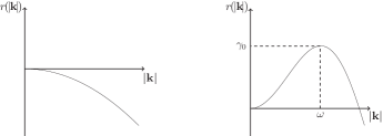
Figure 4: The graph of the function $|\mathbf{k}|\mapsto r(|\mathbf{k}|)$ for $\beta_{0}>\mu_{1}(\mu_{1}\!-\!1)^{2}/(\mu_{1}\!+\!1)$ (left) and $\beta_{0}<\mu_{1}(\mu_{1}\!-\!1)^{2}/(\mu_{1}\!+\!1)$ (right).

Noting that $\ker L_{0}(\omega)=\langle\mathbf{v}\rangle,$ where

$$\mathbf{v}=\left(\begin{array}[]{c}\cfrac{1}{\mu_{1}-1}\left(\mu_{1}S_{1}^{-1}\tanh S_{1}\tilde{\omega}\coth\tilde{\omega}+1\right)\\ -\mu_{1}S_{1}^{-1}\tanh S_{1}\tilde{\omega}\coth\tilde{\omega}\\ 1\\ \end{array}\right),$$ (47)

we find that

$$\ker L_{0}=\langle\left\{\mathbf{v}\sin(\mathbf{k}\cdot\mathbf{x}),\mathbf{v}\cos(\mathbf{k}\cdot\mathbf{x}):\mathbf{k}\in\mathscr{L}^{\star}\ \mathrm{with}\ |\mathbf{k}|=\omega\right\}\rangle$$

(see Figure 5).

1. For rolls the dual lattice $\mathscr{L}^{\star}$ is generated by $\mathbf{k}=(\omega,0),$ so that $|\mathbf{k}|,|-\mathbf{k}|=\omega$ and hence $\dim\ker L_{0}=2$.

2. For rectangles the dual lattice $\mathscr{L}^{\star}$ is generated by $\mathbf{k}_{1}=(\omega,0)$ and $\mathbf{k}_{2}=(0,\omega),$ so that $|\mathbf{k}_{1}|,|-\mathbf{k}_{1}|,|\mathbf{k}_{2}|,|-\mathbf{k}_{2}|=\omega$ and hence $\dim\ker L_{0}=4$.

3. For hexagons the dual lattice $\mathscr{L}^{\star}$ is generated by $\mathbf{k}_{1}=(\omega,0)$ and $\mathbf{k}_{2}=\omega(\frac{1}{2},\frac{\sqrt{3}}{2})$, so that $|\mathbf{k}_{1}|,|-\mathbf{k}_{1}|,|\mathbf{k}_{2}|,|-\mathbf{k}_{2}|,|\mathbf{k}_{3}|,|-\mathbf{k}_{3}|=\omega,$ where $\mathbf{k}_{3}=\mathbf{k}_{2}-\mathbf{k}_{1},$ and hence $\dim\ker L_{0}=6$.

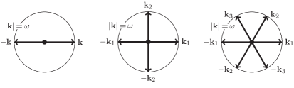
Figure 5: The vectors generated by $\mathscr{L}^{\star}$ with length $\omega$ in the case of rolls (left), rectangles (centre) and hexagons (right).

Define the projection $P_{\omega}:X_{0}\to X_{0},Y_{0}\to Y_{0}$ by

$$P_{\omega}v(\mathbf{x}) =\sum_{\begin{subarray}{c}\mathbf{k}\in\mathscr{L}^{\star},\\ |\mathbf{k}|=\omega\end{subarray}}\mathbf{v}_{{}_{\mathbf{k}}}\mathrm{e}^{\mathrm{i}\mathbf{k}\cdot\mathbf{x}},$$

where $v$ is given by formula (45), so that

$$X_{0}=X_{\omega}\oplus X_{\mathrm{r}},\qquad Y_{0}=Y_{\omega}\oplus Y_{\mathrm{r}}$$

with

$$X_{\omega}=P_{\omega}[X_{0}],\qquad X_{\mathrm{r}}=(I-P_{\omega})[X_{0}],\qquad Y_{\omega}=P_{\omega}[Y_{0}],\qquad Y_{\mathrm{r}}=(I-P_{\omega})[Y_{0}].$$

Using (46), one finds that $\operatorname{Im}L_{0}\big{|}_{X_{\omega}}\subseteq Y_{\omega}$ and $\operatorname{Im}L_{0}\big{|}_{X_{\mathrm{r}}}\subseteq Y_{\mathrm{r}}$ and we prove that $L_{0}:X_{0}\to Y_{0}$ is a Fredholm operator of index zero in two steps.

Lemma 3.1.

The mapping $L_{0}$ is an isomorphism $X_{\mathrm{r}}\to Y_{\mathrm{r}}.$

Proof.

The mapping $L_{0}\big{|}_{X_{\mathrm{r}}}$ is formally invertible on ${Y_{\mathrm{r}}}$ with

$$L_{0}^{-1}(\chi,{{\Psi^{\prime}}},{{\Psi}})^{\mathrm{T}} =\sum_{\begin{subarray}{c}k\in\mathscr{L}^{\star},\\ |\mathbf{k}|\neq\omega\end{subarray}}L_{0}(|\mathbf{k}|)^{-1}(\chi_{{}_{\mathbf{k}}},{{\Psi^{\prime}_{{}_{\mathbf{k}}}}},{{\Psi_{{}_{\mathbf{k}}}}})^{\mathrm{T}}\mathrm{e}^{\mathrm{i}\mathbf{k}\cdot\mathbf{x}},$$ (48)

where

$$L_{0}(|\mathbf{k}|)^{-1} =\frac{\mu_{1}S_{1}^{-1}|\mathbf{k}|\tanh\dfrac{S_{1}|\mathbf{k}|}{\beta_{0}}}{\det L_{0}(|\mathbf{k}|)}\begin{pmatrix}(\mu_{1}-1)|\mathbf{k}|\tanh\dfrac{|\mathbf{k}|}{\beta_{0}}&1&1\\[10.00002pt] -(\gamma_{0}+|\mathbf{k}|^{2})&-(\mu_{1}-1)&-(\mu_{1}-1)\\[10.00002pt] 0&0&0\end{pmatrix}$$

$$\qquad\mbox{}+\frac{|\mathbf{k}|\tanh\dfrac{|\mathbf{k}|}{\beta_{0}}}{\det L_{0}(|\mathbf{k}|)}\begin{pmatrix}0&\mu_{1}&1\\[10.00002pt] 0&0&0\\[10.00002pt] \gamma_{0}+|\mathbf{k}|^{2}&\mu_{1}(\mu_{1}-1)&\mu_{1}-1\end{pmatrix}-\frac{\gamma_{0}+|\mathbf{k}|^{2}}{\det L_{0}(|\mathbf{k}|)}\begin{pmatrix}&0&0&0&\\[10.00002pt] &0&1&0&\\[10.00002pt] &0&1&0&\end{pmatrix}$$

for $\mathbf{k}\in\mathscr{L}^{\star}$ with $|\mathbf{k}|>\omega$ and

$$L_{0}(0)^{-1}\begin{pmatrix}\chi_{{}_{\mathbf{0}}}\\ 0\\ \Psi_{{}_{\mathbf{0}}}\end{pmatrix}=\begin{pmatrix}-\gamma_{0}^{-1}\Psi_{{}_{\mathbf{0}}}\\ 0\\ -\chi_{{}_{\mathbf{0}}}-(\mu_{1}-1)\gamma_{0}^{-1}\Psi_{{}_{\mathbf{0}}}\end{pmatrix}$$

Denoting the right-hand side of equation (48) by $(\eta,\Phi^{\prime},\Phi)^{\mathrm{T}}$ and using the estimates

$${S_{1}^{-1}|\mathbf{k}|\tanh\dfrac{S_{1}|\mathbf{k}|}{\beta_{0}}}\lesssim{|\mathbf{k}|\tanh\dfrac{|\mathbf{k}|}{\beta_{0}}},\qquad\frac{|\mathbf{k}|\tanh\dfrac{|\mathbf{k}|}{\beta_{0}}}{|\det L_{0}(|\mathbf{k}|)|}\lesssim|\mathbf{k}|^{-2}$$

for $|\mathbf{k}|>\omega$, one finds that

$$\left\lVert\eta\right\rVert_{s+{1/2}}^{2} \lesssim\left(|\chi_{{}_{\mathbf{0}}}|+|\Psi_{{}_{\mathbf{0}}}|\right)^{2}+\sum_{\begin{subarray}{c}k\in\mathscr{L}^{\star},\\ |\mathbf{k}|\neq\omega,0\end{subarray}}|\mathbf{k}|^{2s+1}\frac{\left(|\mathbf{k}|\tanh\dfrac{|\mathbf{k}|}{\beta_{0}}\right)^{2}}{(\det L_{0}(|\mathbf{k}|))^{2}}\left(|\mathbf{k}|\tanh\dfrac{|\mathbf{k}|}{\beta_{0}}\ |\chi_{{}_{\mathbf{k}}}|+|\Psi^{\prime}_{{}_{\mathbf{k}}}|+|\Psi_{{}_{\mathbf{k}}}|\right)^{2}$$

$$\lesssim|\chi_{{}_{\mathbf{0}}}|^{2}+|\Psi_{{}_{\mathbf{0}}}|^{2}+\sum_{\begin{subarray}{c}k\in\mathscr{L}^{\star},\\ |\mathbf{k}|\neq\omega,0\end{subarray}}|\mathbf{k}|^{2s-3}\left(|\mathbf{k}|^{2}|\chi_{{}_{\mathbf{k}}}|^{2}+|\Psi^{\prime}_{{}_{\mathbf{k}}}|^{2}+|\Psi_{{}_{\mathbf{k}}}|^{2}\right)$$

$$\lesssim\left\lVert\chi\right\rVert_{s}^{2}+\left\lVert{{\Psi^{\prime}}}\right\rVert_{s-1}^{2}+\left\lVert{{\Psi}}\right\rVert_{s-{3/2}}^{2};$$

similar calculations yield

$$\left\lVert\Phi^{\prime}\right\rVert_{s}^{2}\lesssim\left\lVert\chi\right\rVert_{s}^{2}+\left\lVert{{\Psi^{\prime}}}\right\rVert_{s-1}^{2}+\left\lVert{{\Psi}}\right\rVert_{s-{3/2}}^{2},\qquad\left\lVert\Phi\right\rVert_{s}^{2}\lesssim\left\lVert\chi\right\rVert_{s}^{2}+\left\lVert{{\Psi^{\prime}}}\right\rVert_{s-1}^{2}+\left\lVert{{\Psi}}\right\rVert_{s-{3/2}}^{2}.$$

We conclude that $L_{0}^{-1}:Y_{\mathrm{r}}\to X_{\mathrm{r}}$ exists and is continuous. ∎

Corollary 3.1.

The operator $L_{0}:X_{0}\to Y_{0}$ is a Fredholm operator of index zero.

Proof.

A straightforward calculation shows that $\mathbf{v}\notin\operatorname{Im}{L_{0}(\omega)}$ (so that $\ker(L_{0}(\omega))^{2}=\ker L_{0}(\omega)$) and hence

$$Y_{\omega} =\bigoplus_{\begin{subarray}{c}\mathbf{k}\in\mathscr{L}^{\star},\\ |\mathbf{k}|=\omega\end{subarray}}\Big{(}\big{(}\operatorname{Im}{L_{0}(\omega)}\oplus\ker L_{0}(\omega)\big{)}\sin(\mathbf{k}\cdot\mathbf{x})\oplus\big{(}\operatorname{Im}{L_{0}(\omega)}\oplus\ker L_{0}(\omega)\big{)}\cos\textbullet\cdot\mathbf{x})\Big{)}$$

$$=\operatorname{Im}{L_{0}}\big{|}_{X_{\omega}}\oplus\ker L_{0}.$$

Using this decomposition and Lemma 3.1, we find that

$$Y_{0}=Y_{\omega}\oplus Y_{\mathrm{r}}=\left(\operatorname{Im}{L_{0}}\big{|}_{X_{\omega}}\oplus\ker L_{0}\right)\oplus\operatorname{Im}L_{0}\big{|}_{U_{\mathrm{r}}}=\operatorname{Im}L_{0}\oplus\ker L_{0}.$$

It follows that $\operatorname{Im}L_{0}$ is closed and $\mathrm{codim}\,\operatorname{Im}L_{0}=\dim\ker L_{0},$ so that $L_{0}:X_{0}\to Y_{0}$ is a Fredholm operator of index zero. ∎

Because the kernel of $L_{0}$ is multidimensional, we can not use Theorem 3.1 directly. To overcome this problem, we recall that ${\mathcal{G}}$ (and hence $L_{0}$) is invariant under certain rotations (see below) and seek solutions to (43) in $X_{0}$ that have this rotational symmetry, denoting the relevant subspaces of $H^{r}_{\mathrm{per}}(\Gamma),\bar{H}^{r}_{\mathrm{per}}(\Gamma),X_{0}$ and $Y_{0}$ by $H^{r}_{\mathrm{sym}}(\Gamma),\bar{H}^{r}_{\mathrm{sym}}(\Gamma),X_{\mathrm{sym}}$ and $Y_{\mathrm{sym}},$ so that

$$X_{\mathrm{sym}}=H^{s+{1/2}}_{\mathrm{sym}}(\Gamma)\times\bar{H}^{s}_{\mathrm{sym}}(\Gamma)\times H^{s}_{\mathrm{sym}}(\Gamma),\qquad Y_{\mathrm{sym}}=H^{s}_{\mathrm{sym}}(\Gamma)\times\bar{H}^{s-1}_{\mathrm{sym}}(\Gamma)\times H^{s-{3/2}}_{\mathrm{sym}}(\Gamma)$$

for $s>{5/2}$. Note that $X_{\mathrm{sym}}$ and $Y_{\mathrm{sym}}$ are invariant under $P_{\omega}$, so that according to the above analysis $L_{0}:X_{\mathrm{sym}}\to Y_{\mathrm{sym}}$ is a Fredholm operator of index zero and

$$Y_{\mathrm{sym}}=\operatorname{Im}L_{0}\oplus\ker L_{0}.$$

1. For rolls we consider functions that are independent of the $z$-coordinate and lie in the subspace

   $$H^{r}_{\mathrm{sym}}(\Gamma)=\left\{\zeta\in H^{r}_{\mathrm{per}}(\Gamma):\ \zeta\left(x\right)=\zeta\left(-x\right)\right\}$$

   of functions which are invariant under rotations through $\pi.$

2. For rectangles we work with the subspace

   $$H^{r}_{\mathrm{sym}}(\Gamma)=\left\{\zeta\in H^{r}_{\mathrm{per}}(\Gamma):\ \zeta\left(x,z\right)=\zeta\left(z,-x\right)\right\}$$

   of functions which are invariant under rotations through ${\pi/2}.$

3. For hexagons we work with the subspace

   $$H^{r}_{\mathrm{sym}}(\Gamma)=\left\{\zeta\in H^{r}_{\mathrm{per}}(\Gamma):\ \zeta\left(x,z\right)=\zeta\left(\frac{1}{2}\left(x-\sqrt{3}z\right),\frac{1}{2}\left(\sqrt{3}x+z\right)\right)\right\}$$

   of functions which are invariant under rotations through ${\pi/3}.$

These restrictions ensure that $\dim\ker L_{0}=1$ with $\ker L_{0}=\langle v_{0}\rangle,$ where $v_{0}=\mathbf{v}e_{1}(x,z)$ with

$$e_{1}(x,z)=\left\{\begin{array}[]{ll}\cos\omega x&\qquad\mbox{(rolls)}\\ \cos\omega x+\cos\omega z&\qquad\mbox{(rectangles)}\\ \cos\omega x+\cos\frac{\omega}{2}\left(x+\sqrt{3}z\right)+\cos\frac{\omega}{2}\left(x-\sqrt{3}z\right)&\qquad\mbox{(hexagons).}\end{array}\right.$$

The projection $P:Y_{\mathrm{sym}}\to Y_{\mathrm{sym}}$ onto $\ker L_{0}$ along $\operatorname{Im}L_{0}$ is given by

$$P(\chi,\Psi^{\prime},\Psi)^{\mathrm{T}}={C^{\star}}((\chi_{{}_{(\omega,0)}},\Psi^{\prime}_{{}_{(\omega,0)}},\Psi_{{}_{(\omega,0)}})^{\mathrm{T}}\cdot\mathbf{v}^{\star})\mathbf{v}\,e_{1}(x,z),$$ (49)

where

$$\mathbf{v}^{\star}=\left(\begin{array}[]{c}\cfrac{\gamma_{0}+\omega^{2}}{\mu_{1}-1}\\ \cfrac{\gamma_{0}+\omega^{2}}{(\mu_{1}-1)^{2}\omega}\left(S_{1}^{-1}\coth S_{1}\tilde{\omega}+\coth\tilde{\omega}\right)\\ 1\\ \end{array}\right),$$

$$C^{\star}=\mu_{1}\omega S_{1}^{-1}\tanh S_{1}\tilde{\omega}-\mu_{1}^{2}S_{1}^{-1}\dfrac{\tanh S_{1}\tilde{\omega}\big{(}\coth\tilde{\omega}+S_{1}\coth S_{1}\tilde{\omega}\big{)}}{\tanh\tilde{\omega}\big{(}\mu_{1}\coth\tilde{\omega}+S_{1}\coth S_{1}\tilde{\omega}\big{)}}+1$$

($\mathbf{v}^{\star}\in\mathbb{R}^{3}$ solves the equation $L_{0}(\omega)^{\mathrm{T}}\mathbf{v}^{\star}=\mathbf{0}$ and $C^{\star}=(\mathbf{v}\cdot\mathbf{v}^{\star})^{-1}$).

Lemma 3.2.

The transversality condition $P(\mathrm{d}_{1}\mathrm{d}_{2}{\mathcal{G}}[\gamma_{0},0](1,v_{0}))\neq 0$ is satisfied.

Proof.

It follows from the calculation $\mathrm{d}_{1}\mathrm{d}_{2}{\mathcal{G}}[\gamma_{0},0](1,(\eta,\Phi^{\prime},\Phi)^{\mathrm{T}})=(0,0,-\eta)^{\mathrm{T}}$ and the formula (49) for $P$ that

$$\hskip 9.95863ptP(\mathrm{d}_{1}\mathrm{d}_{2}{\mathcal{G}}[\gamma_{0},0](1,v_{0}))=-C^{\star}(\mu_{1}-1)^{-1}S_{1}^{-1}\tanh S_{1}\tilde{\omega}(\mu_{1}\coth\tilde{\omega}+S_{1}\coth S_{1}\tilde{\omega})\mathbf{v}\,e_{1}(x,z).\hskip 9.10509pt\qed$$

The facts established above confirm that the hypotheses of Theorem 3.1 are satisfied, an application of which yields Theorem 1.1.

4 The bifurcating solution branches

In this section we examine the bifurcating solution branches identified in Theorem 1.1 by applying the following supplement to the Crandall-Rabinowitz theorem.

Theorem 4.1.

Suppose that the hypotheses of Theorem 3.1 hold. In the notation of that theorem, let $Q:X\rightarrow X$ be a projection with $\operatorname{Im}Q=\ker L$ and the Taylor series of the functions $w:(-\varepsilon,\varepsilon)\rightarrow V,$ $\lambda:(-\varepsilon,\varepsilon)\rightarrow\mathbb{R}$ be given by

$$\lambda(s)=\lambda_{{{0}}}+s\lambda_{{{1}}}+s^{2}\lambda_{{{2}}}+\ldots,\qquad w(s)=v_{0}+sw_{1}+\ldots,$$

where $\lambda_{{{1}}},\lambda_{{{2}}},\ldots\in\mathbb{R}$ and $w_{1},w_{2},\ldots\in\ker Q.$

1. The coefficient $\lambda_{{{1}}}$ satisfies the equation

   $$P\left(\frac{1}{2!}{\mathrm{d}_{2}^{2}{\mathcal{F}}[\lambda_{{{0}}},0]({v_{0},v_{0}}})\right)+\lambda_{{{1}}}P(\mathrm{d}_{1}\mathrm{d}_{2}{\mathcal{F}}[\lambda_{{{0}}},0](1,v_{0}))=0$$

   and the bifurcation is transcritical if $\lambda_{{{1}}}$ is non-zero (see Figure 6).

   

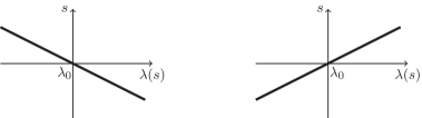
   Figure 6: Transcritical Crandall-Rabinowitz bifurcation for $\lambda_{1}<0$ (left) and $\lambda_{1}>0$ (right).

2. Suppose that $\lambda_{{{1}}}$ is zero. The coefficient $\lambda_{{{2}}}$ satisfies the equation

   $$P\left({\mathrm{d}_{2}^{2}{\mathcal{F}}[\lambda_{{{0}}},0](v_{0},w_{1})}+\frac{1}{3!}\mathrm{d}_{2}^{3}{\mathcal{F}}[\lambda_{{{0}}},0](v_{0},v_{0},v_{0})\right)+\lambda_{{{2}}}P\left(\mathrm{d}_{1}\mathrm{d}_{2}{\mathcal{F}}[\lambda_{{{0}}},0](1,v_{0})\right)=0,$$

   where $w_{1}\in\ker Q$ solves the equation

   $$\mathrm{d}_{2}{\mathcal{F}}[\lambda_{{{0}}},0](w_{1})=-\frac{1}{2!}\mathrm{d}_{2}^{2}{\mathcal{F}}[\lambda_{{{0}}},0](v_{0},v_{0}).$$

   The bifurcation is supercritical for $\lambda_{{{2}}}>0$ and subcritical for $\lambda_{{{2}}}<0$ (see Figure 7).

   

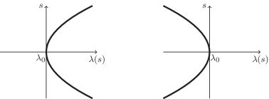
   Figure 7: Crandall-Rabinowitz bifurcation for $\lambda_{{{1}}}=0$, $\lambda_{{{2}}}>0$ (supercritical, left) and $\lambda_{{{1}}}=0$, $\lambda_{{{2}}}<0$ (subcritical,right).

To apply this theorem we write the Taylor series of the analytic functions $w:(-\varepsilon,\varepsilon)\rightarrow V_{\mathrm{sym}}$, $\gamma:(-\varepsilon,\varepsilon)\rightarrow\mathbb{R}$ given in Theorem 1.1 as

$$\gamma(s)=\gamma_{0}+s\gamma_{1}+s^{2}\gamma_{2}+\ldots,\qquad w(s)=v_{0}+sw_{1}+\ldots$$

with $\gamma_{1},\gamma_{2},\ldots\in\mathbb{R}$ and $w_{1},w_{2},\ldots\in\ker(I-P)$ and introduce the operators

$$L_{1}=\mathrm{d}_{1}\mathrm{d}_{2}{\mathcal{G}}[\gamma_{0},0](1,\cdot),\qquad Q_{0}=\frac{1}{2!}\mathrm{d}_{2}^{2}{\mathcal{G}}[\gamma_{0},0],\qquad C_{0}=\frac{1}{3!}\mathrm{d}_{2}^{3}{\mathcal{G}}[\gamma_{0},0].$$

One finds that $L_{1}(v)=(0,0,-\eta)^{\mathrm{T}}$ and

$$Q_{0} (v,v)$$

$$=\begin{pmatrix}0\\[10.00002pt] G_{2}^{\prime}+G_{2}+\dot{\mu}_{1}H_{2}+\tfrac{1}{2}\left(\ddot{\mu}_{1}H_{1}^{2}+\dot{\mu}_{1}|\nabla\Phi|^{2}\right)\\[10.00002pt] \tfrac{1}{2}\left(G^{\prime\,2}_{1}\!-|\nabla\Phi^{\prime}|^{2}+(\mu_{1}-\dot{\mu}_{1})H_{1}^{2}+\mu_{1}|\nabla\Phi|^{2}-2G_{1}H_{1}-\ddot{\mu}_{1}H_{1}^{2}-\dot{\mu}_{1}|\nabla\Phi|^{2}\right)\\ -\mu_{1}G_{2}^{\prime}-G_{2}-\dot{\mu}_{1}H_{2}\end{pmatrix}$$

$$C_{0} (v,v,v)$$

$$=\begin{pmatrix}0\\[15.00002pt] G_{3}^{\prime}+G_{3}+\dot{\mu}_{1}H_{3}+\ddot{\mu}_{1}H_{1}H_{2}+\tfrac{1}{2}\left(\ddot{\mu}_{1}-\dot{\mu}_{1}\right)|\nabla\Phi|^{2}H_{1}-\dot{\mu}_{1}\nabla\eta\cdot\nabla\Phi\ H_{1}+\tfrac{1}{6}{\mathop{\kern 0.0pt\mu}\limits^{\makebox[0.0pt][c]{\vbox to-2.0pt{\kern-2.0pt\hbox{\scalebox{0.89}{.}\kern-0.5pt\scalebox{0.89}{.}\kern-0.5pt\scalebox{0.89}{.}}\vss}}}}_{1}H_{1}^{3}\\[15.00002pt] -\mu_{1}G_{3}^{\prime}-G_{3}-\dot{\mu}_{1}H_{3}-\ddot{\mu}_{1}H_{1}H_{2}-\tfrac{1}{2}\left(\ddot{\mu}_{1}-\dot{\mu}_{1}\right)|\nabla\Phi|^{2}H_{1}+\dot{\mu}_{1}\nabla\eta\cdot\nabla\Phi\ H_{1}-\tfrac{1}{6}{\mathop{\kern 0.0pt\mu}\limits^{\makebox[0.0pt][c]{\vbox to-2.0pt{\kern-2.0pt\hbox{\scalebox{0.89}{.}\kern-0.5pt\scalebox{0.89}{.}\kern-0.5pt\scalebox{0.89}{.}}\vss}}}}_{1}H_{1}^{3}\\[2.5pt] +G_{1}^{\prime}(G_{2}^{\prime}-\nabla\eta\cdot\nabla\Phi^{\prime})-H_{1}(G_{2}+\mu_{1}\nabla\eta\cdot\nabla\Phi)+(\mu_{1}-\dot{\mu}_{1})H_{1}H_{2}+\tfrac{1}{3}(\dot{\mu}_{1}-\ddot{\mu}_{1})H_{1}^{3}\\[2.5pt] -G_{1}H_{2}+\eta_{x}^{2}\eta_{zz}+\eta_{z}^{2}\eta_{xx}-2\eta_{x}\eta_{z}\eta_{xz}-\tfrac{3}{2}|\nabla\eta|^{2}\eta\end{pmatrix},$$

where $v=(\eta,\Phi^{\prime},\Phi)^{\mathrm{T}}$ and ${\mathop{\kern 0.0pt\mu}\limits^{\makebox[0.0pt][c]{\vbox to-2.0pt{\kern-2.0pt\hbox{\scalebox{0.89}{.}\kern-0.5pt\scalebox{0.89}{.}\kern-0.5pt\scalebox{0.89}{.}}\vss}}}}_{1}={\mathop{\kern 0.0pt\mu}\limits^{\makebox[0.0pt][c]{\vbox to-2.0pt{\kern-2.0pt\hbox{\scalebox{0.89}{.}\kern-0.5pt\scalebox{0.89}{.}\kern-0.5pt\scalebox{0.89}{.}}\vss}}}}(1)$. Theorem 4.1 shows that

$$\gamma_{1}=-\frac{\left[{Q_{0}(v_{0},v_{0})}\right]_{1}\cdot\mathbf{v}^{\star}}{\left[{L_{1}v_{0}}\right]_{1}\cdot\mathbf{v}^{\star},}$$

where

$$\left[\zeta\right]_{1}={\zeta}_{{}_{(\omega,0)}}=\int_{\Gamma}\zeta e_{1}$$

(with componentwise extension), and

$$\gamma_{2} =-\frac{\left[{2Q_{0}(v_{0},w_{1})+C_{0}(v_{0},v_{0},v_{0})}\right]_{1}\cdot\mathbf{v}^{\star}}{\left[{L_{1}v_{0}}\right]_{1}\cdot\mathbf{v}^{\star}}$$

for $\gamma_{1}=0$, where $w_{1}\in\ker(I-P)$ solves the equation

$$L_{0}w_{1} =-Q_{0}(v_{0},v_{0}).$$

A straightforward calculation shows $Q_{0}(v_{0},v_{0})$ can be written as a sum in which each summand is a constant vector multiplied by either $e_{1}^{2}$ or $|\nabla e_{1}|^{2}$. For hexagons we find that $\gamma_{1}$ generally does not vanish, while for rolls

$$\left[{e_{1}^{2}}\right]_{1}=\left[{\frac{1}{2}+\frac{1}{2}\cos 2\omega x}\right]_{1}=0,\qquad\left[{|\nabla e_{1}|^{2}}\right]_{1}=\left[{\frac{1}{2}-\frac{1}{2}\cos 2\omega x}\right]_{1}=0,$$

and for rectangles

$$\left[e_{1}^{2}\right]_{1} =\left[\frac{1}{2}+{\cos\omega(x+z)+\cos\omega(x-z)}+\frac{1}{2}({\cos 2\omega x+\cos 2\omega z)}\right]_{1}=0,$$

$$\left[|\nabla e_{1}|^{2}\right]_{1} =\left[1-\frac{1}{2}({\cos 2\omega x\ +\cos 2\omega z)}\right]_{1}=0,$$

so that in both cases $\gamma_{1}=0$. Attempting to compute explicit general expressions for $\gamma_{2}$ leads to unwieldy formulae (it appears more appropriate to calculate them numerically for a specific choice of $\mu$, that is a specific magnetisation law). Here we confine ourselves to stating the values of the coefficients for two particular special cases.

1. Constant relative permeability $\mu$ (corresponding to a linear magnetisation law): We find that

   $$\gamma_{2} =-\mu\frac{\mu-1}{\mu+1}\omega^{2}\Bigg{(}\!\!\!-\mu C_{2}\bigg{(}\bigg{(}8(\mu+1)\omega^{2}\frac{4\omega^{2}+\gamma_{0}}{t_{2}}-4(\mu^{2}-1)^{2}\omega^{3}\bigg{)}(1-t_{1}t_{2})^{2}$$

   $$\hskip 97.56493pt\mbox{}+\omega^{3}(\mu-1)^{4}\bigg{(}2(1+t_{1}^{2})(1-t_{1}t_{2})-\frac{1}{4}(1+t_{1}^{2})^{2}\bigg{)}\bigg{)}$$

   $$\hskip 61.42993pt\mbox{}-\frac{\mu\omega^{2}}{4\gamma_{0}}\frac{(\mu-1)^{3}}{\mu+1}(1-t_{1}^{2})^{2}-\frac{(\mu+1)^{2}\omega}{\mu-1}t_{1}\bigg{(}\frac{3\ \omega^{2}}{8(\gamma_{0}+\omega^{2})}-\frac{3}{2}+t_{1}t_{2}\bigg{)}\!\!\Bigg{)}$$

   for rolls and

   $$\gamma_{2} =-\mu\frac{\mu-1}{\mu+1}\omega^{2}\Bigg{(}\!\!\!-\mu C_{\sqrt{2}}\bigg{(}\bigg{(}8(\mu+1)\omega^{2}\frac{2\omega^{2}+\gamma_{0}}{t_{\sqrt{2}}}-2\sqrt{2}(\mu^{2}-1)^{2}\omega^{3}\bigg{)}(1-\sqrt{2}t_{1}t_{\sqrt{2}})^{2}$$

   $$\hskip 104.79128pt\mbox{}-\frac{\omega^{3}(\mu-1)^{4}}{2}\sqrt{2}\bigg{(}t_{1}^{4}-4t_{1}^{2}(1-\sqrt{2}t_{1}t_{\sqrt{2}})\bigg{)}\bigg{)}$$

   $$\hskip 61.42993pt\mbox{}-\mu C_{2}\bigg{(}\bigg{(}8(\mu+1)\omega^{2}\frac{4\omega^{2}+\gamma_{0}}{t_{2}}-4(\mu^{2}-1)^{2}\omega^{3}\bigg{)}(1-t_{1}t_{2})^{2}$$

   $$\hskip 97.56493pt\mbox{}+\omega^{3}(\mu-1)^{4}\bigg{(}2(1+t_{1}^{2})(1-t_{1}t_{2})-\frac{1}{4}(1+t_{1}^{2})^{2}\bigg{)}\bigg{)}$$

   $$\hskip 61.42993pt\mbox{}-\frac{\omega(\mu+1)^{2}}{2(\mu-1)}t_{1}\bigg{(}\frac{5\omega^{2}}{4(\gamma_{0}+\omega^{2})}\!-\!9\!+2t_{1}t_{2}\!+\!4\sqrt{2}t_{1}t_{\sqrt{2}}\bigg{)}$$

   $$\hskip 61.42993pt-\frac{\omega^{2}\mu(\mu-1)^{3}}{2\gamma_{0}(\mu+1)}(1-t_{1}^{2})^{2}\Bigg{)}$$

   for rectangles, where $t_{1}=\tanh\tilde{\omega}$, $t_{{}_{\sqrt{2}}}=\tanh\sqrt{2}\tilde{\omega}$, $t_{2}=\tanh 2\tilde{\omega}$, $\tilde{\omega}=\omega/\beta_{0}$ and

   $$C_{{}_{\sqrt{2}}} =\frac{1}{\sqrt{2}(\mu^{2}-1)\omega}\left(\sqrt{2}(\omega^{2}+\gamma_{0})\frac{t_{\sqrt{2}}}{t_{1}}-\gamma_{0}-2\omega^{2}\right)^{-1},$$

   $$C_{2} =\frac{1}{2(\mu^{2}-1)\omega}\left(2(\gamma_{0}+\omega^{2})\frac{t_{2}}{t_{1}}-\gamma_{0}-4\omega^{2}\right)^{-1}$$

   The sign of $\gamma_{2}$ clearly depends upon $\mu$ and $\tilde{\omega}$ (see Figure 8).

   

   

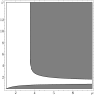
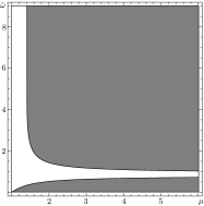
   Figure 8: The sign of the coefficient $\gamma_{2}$ as a function of $\mu$ and $\tilde{\omega}$ for a linear magnetisation law for rolls (left) and rectangles (right). The shaded and white areas show the regions in which the bifurcation is respectively super- and subcritical.

2. Small values of $\beta_{0}$ (corresponding to deep fluids): Abbreviating $\mu(1),\dot{\mu}(1),\ddot{\mu}(1),{\mathop{\kern 0.0pt\mu}\limits^{\makebox[0.0pt][c]{\vbox to-2.0pt{\kern-2.0pt\hbox{\scalebox{0.89}{.}\kern-0.5pt\scalebox{0.89}{.}\kern-0.5pt\scalebox{0.89}{.}}\vss}}}}(1)$ to respectively $\mu_{1},\dot{\mu}_{1},\ddot{\mu}_{1},{\mathop{\kern 0.0pt\mu}\limits^{\makebox[0.0pt][c]{\vbox to-2.0pt{\kern-2.0pt\hbox{\scalebox{0.89}{.}\kern-0.5pt\scalebox{0.89}{.}\kern-0.5pt\scalebox{0.89}{.}}\vss}}}}_{1}$, one finds that

   $$\gamma_{2} =\Big{(}t\big{(}2\mu_{1}^{3}{\mathop{\kern 0.0pt\mu}\limits^{\makebox[0.0pt][c]{\vbox to-2.0pt{\kern-2.0pt\hbox{\scalebox{0.89}{.}\kern-0.5pt\scalebox{0.89}{.}\kern-0.5pt\scalebox{0.89}{.}}\vss}}}}_{1}+2\mu_{1}^{2}\dot{\mu}_{1}{\mathop{\kern 0.0pt\mu}\limits^{\makebox[0.0pt][c]{\vbox to-2.0pt{\kern-2.0pt\hbox{\scalebox{0.89}{.}\kern-0.5pt\scalebox{0.89}{.}\kern-0.5pt\scalebox{0.89}{.}}\vss}}}}_{1}-2\mu_{1}^{2}{\mathop{\kern 0.0pt\mu}\limits^{\makebox[0.0pt][c]{\vbox to-2.0pt{\kern-2.0pt\hbox{\scalebox{0.89}{.}\kern-0.5pt\scalebox{0.89}{.}\kern-0.5pt\scalebox{0.89}{.}}\vss}}}}_{1}-2\mu_{1}\dot{\mu}_{1}{\mathop{\kern 0.0pt\mu}\limits^{\makebox[0.0pt][c]{\vbox to-2.0pt{\kern-2.0pt\hbox{\scalebox{0.89}{.}\kern-0.5pt\scalebox{0.89}{.}\kern-0.5pt\scalebox{0.89}{.}}\vss}}}}_{1}-\tfrac{11}{2}\mu_{1}^{2}{\ddot{\mu}_{1}}^{2}+\tfrac{11}{2}\mu_{1}\ddot{\mu}_{1}^{2}+42\mu_{1}^{3}\ddot{\mu}_{1}+49\mu_{1}^{2}\dot{\mu}_{1}\ddot{\mu}_{1}-8\mu_{1}^{2}\dot{\mu}_{1}$$

   $$\qquad\qquad\mbox{}+29\mu_{1}{\dot{\mu}_{1}}^{2}\ddot{\mu}_{1}-10\mu_{1}^{2}\ddot{\mu}_{1}+15\mu_{1}\dot{\mu}_{1}\ddot{\mu}_{1}+3{\dot{\mu}_{1}}^{2}\ddot{\mu}_{1}+8\dot{\mu}_{1}\mu_{1}^{3}+16\mu_{1}^{2}{\dot{\mu}_{1}}^{2}+8\mu_{1}{\dot{\mu}_{1}}^{3}-16\mu_{1}{\dot{\mu}_{1}}^{2}-8{\dot{\mu}_{1}}^{3}\big{)}$$

   $$\qquad\mbox{}+16\mu_{1}^{4}\ddot{\mu}_{1}+32\mu_{1}^{3}\dot{\mu}_{1}\ddot{\mu}_{1}+16\mu_{1}^{2}\dot{\mu}_{1}^{2}\ddot{\mu}_{1}+30\mu_{1}^{2}\dot{\mu}_{1}\ddot{\mu}_{1}+5\mu_{1}^{2}{\ddot{\mu}_{1}}^{2}+10\mu_{1}{\dot{\mu}_{1}}^{2}\ddot{\mu}_{1}-16\mu_{1}^{2}\ddot{\mu}_{1}-46\mu_{1}\dot{\mu}_{1}\ddot{\mu}_{1}$$

   $$\qquad\mbox{}-5\mu_{1}\ddot{\mu}_{1}^{2}-10{\dot{\mu}_{1}}^{2}\ddot{\mu}_{1}\Big{)}\frac{(\mu_{1}-1)^{7}\mu_{1}^{2}}{512t^{6}(\mu_{1}+\dot{\mu}_{1})}$$

   $$\quad+\Big{(}t\big{(}96\mu_{1}^{6}+636\mu_{1}^{5}\dot{\mu}_{1}+1129\mu_{1}^{4}{\dot{\mu}_{1}}^{2}+850\mu_{1}^{3}{\dot{\mu}_{1}}^{3}+217\mu_{1}^{2}{\dot{\mu}_{1}}^{4}-512\mu_{1}^{5}-1720\mu_{1}^{4}\dot{\mu}_{1}-1810\mu_{1}^{3}{\dot{\mu}_{1}}^{2}$$

   $$\qquad\qquad\quad\mbox{}-740\mu_{1}^{2}{\dot{\mu}_{1}}^{3}-50\mu_{1}{\dot{\mu}_{1}}^{4}+96\mu_{1}^{4}+220\dot{\mu}_{1}\mu_{1}^{3}+73\mu_{1}^{2}{\dot{\mu}_{1}}^{2}-14\mu_{1}{\dot{\mu}_{1}}^{3}-7{\dot{\mu}_{1}}^{4}\big{)}$$

   $$\qquad\quad\mbox{}+88\mu_{1}^{8}+440\mu_{1}^{7}\dot{\mu}_{1}+880\mu_{1}^{6}{\dot{\mu}_{1}}^{2}+880\mu_{1}^{5}{\dot{\mu}_{1}}^{3}+440\mu_{1}^{4}{\dot{\mu}_{1}}^{4}+88\mu_{1}^{3}{\dot{\mu}_{1}}^{5}-\!256\!\mu_{1}^{7}\!-\!928\mu_{1}^{6}\dot{\mu}_{1}\!-\!1312\mu_{1}^{5}{\dot{\mu}_{1}}^{2}$$

   $$\qquad\quad\mbox{}-864\mu_{1}^{4}{\dot{\mu}_{1}}^{3}-224\mu_{1}^{3}{\dot{\mu}_{1}}^{4}-80\mu_{1}^{6}-416\mu_{1}^{5}\dot{\mu}_{1}-614\mu_{1}^{4}{\dot{\mu}_{1}}^{2}-420\mu_{1}^{3}{\dot{\mu}_{1}}^{3}-102\mu_{1}^{2}{\dot{\mu}_{1}}^{4}\!+\!256\mu_{1}^{5}\!+\!672\mu_{1}^{4}\dot{\mu}_{1}$$

   $$\qquad\quad\mbox{}-8\mu_{1}^{4}+460\mu_{1}^{3}{\dot{\mu}_{1}}^{2}\!+\!104\mu_{1}^{2}{\dot{\mu}_{1}}^{3}-20\mu_{1}{\dot{\mu}_{1}}^{4}\!+\!72\dot{\mu}_{1}\mu_{1}^{3}\!+\!194\mu_{1}^{2}{\dot{\mu}_{1}}^{2}\!+\!84\mu_{1}{\dot{\mu}_{1}}^{3}\!+\!10{\dot{\mu}_{1}}^{4}\Big{)}\!\frac{(\mu_{1}-1)^{6}\mu_{1}}{1024t^{6}(\mu_{1}+\dot{\mu}_{1})}$$

   $$\quad+o(1)$$

   as $\beta_{0}\rightarrow 0$ for rolls and

   $${\gamma_{2}} =\Big{(}t\big{(}(42\sqrt{2}\!-\!60)\mu_{1}{\mathop{\kern 0.0pt\mu}\limits^{\makebox[0.0pt][c]{\vbox to-2.0pt{\kern-2.0pt\hbox{\scalebox{0.89}{.}\kern-0.5pt\scalebox{0.89}{.}\kern-0.5pt\scalebox{0.89}{.}}\vss}}}}_{1}\dot{\mu}_{1}\!-\!(42\sqrt{2}\!-\!60)\mu_{1}^{2}{\mathop{\kern 0.0pt\mu}\limits^{\makebox[0.0pt][c]{\vbox to-2.0pt{\kern-2.0pt\hbox{\scalebox{0.89}{.}\kern-0.5pt\scalebox{0.89}{.}\kern-0.5pt\scalebox{0.89}{.}}\vss}}}}_{1}\dot{\mu}_{1}+(\!{\tfrac{411}{\sqrt{2}}}\!-\!289)\mu_{1}\ddot{\mu}_{1}^{2}+\!(4461\sqrt{2}\!-\!6190)\ddot{\mu}_{1}\mu_{1}^{2}\dot{\mu}_{1}$$

   $$\qquad\qquad\mbox{}+\!(3413\sqrt{2}\!-\!4766)\ddot{\mu}_{1}\mu_{1}\dot{\mu}_{1}^{2}\!-\!(429\sqrt{2}\!-\!558)\ddot{\mu}_{1}\mu_{1}\dot{\mu}_{1}+\!(168\sqrt{2}\!-\!240)\dot{\mu}_{1}^{3}+\!(168\sqrt{2}\!-\!240)\mu_{1}^{2}\dot{\mu}_{1}$$

   $$\qquad\qquad\mbox{}+\!(336\sqrt{2}\!-\!480)\mu_{1}\dot{\mu}_{1}^{2}+\!(1870\sqrt{2}\!-\!2580)\ddot{\mu}_{1}\mu_{1}^{3}+\!(82\sqrt{2}\!-\!172)\ddot{\mu}_{1}\mu_{1}^{2}\!-\!\!(1333\sqrt{2}\!-\!1886)\ddot{\mu}_{1}\dot{\mu}_{1}^{2}$$

   $$\qquad\qquad\mbox{}+\!(42\sqrt{2}\!-\!60)\mu_{1}^{2}{\mathop{\kern 0.0pt\mu}\limits^{\makebox[0.0pt][c]{\vbox to-2.0pt{\kern-2.0pt\hbox{\scalebox{0.89}{.}\kern-0.5pt\scalebox{0.89}{.}\kern-0.5pt\scalebox{0.89}{.}}\vss}}}}_{1}\!-\!(\!{\tfrac{411}{\sqrt{2}}\!}\!-\!289)\mu_{1}^{2}\ddot{\mu}_{1}^{2}\!-\!(168\sqrt{2}\!-\!240)\mu_{1}\dot{\mu}_{1}^{3}\!-\!(168\sqrt{2}\!-\!240)\dot{\mu}_{1}\mu_{1}^{3}$$

   $$\qquad\qquad\mbox{}\!-\!(336\sqrt{2}\!-\!480)\mu_{1}^{2}\dot{\mu}_{1}^{2}\!-\!(42\sqrt{2}\!-\!60)\mu_{1}^{3}{\mathop{\kern 0.0pt\mu}\limits^{\makebox[0.0pt][c]{\vbox to-2.0pt{\kern-2.0pt\hbox{\scalebox{0.89}{.}\kern-0.5pt\scalebox{0.89}{.}\kern-0.5pt\scalebox{0.89}{.}}\vss}}}}_{1}\big{)}$$

   $$\qquad\mbox{}+\!(976\sqrt{2}\!-\!1376)\mu_{1}^{4}\ddot{\mu}_{1}+\!(1952\sqrt{2}\!-\!2752)\dot{\mu}_{1}\mu_{1}^{3}\ddot{\mu}_{1}+\!(976\sqrt{2}\!-\!1376)\mu_{1}^{2}\dot{\mu}_{1}^{2}\ddot{\mu}_{1}+\!(445\sqrt{2}\!-\!622)\mu_{1}^{2}\ddot{\mu}_{1}^{2}$$

   $$\qquad\mbox{}+\!(366\sqrt{2}\!-\!468)\mu_{1}^{2}\dot{\mu}_{1}\ddot{\mu}_{1}\!-\!(1414\sqrt{2}\!-\!2020)\mu_{1}\dot{\mu}_{1}^{2}\ddot{\mu}_{1}\!-\!(445\sqrt{2}\!-\!622)\mu_{1}\ddot{\mu}_{1}^{2}\!-\!(976\sqrt{2}\!-\!1376)\mu_{1}^{2}\ddot{\mu}_{1}$$

   $$\qquad\mbox{}\!-\!(1342\sqrt{2}\!-\!1844)\mu_{1}\dot{\mu}_{1}\ddot{\mu}_{1}+\!(1414\sqrt{2}\!-\!2020)\dot{\mu}_{1}^{2}\ddot{\mu}_{1}\Big{)}\frac{(\mu_{1}\!-\!1)^{7}\mu_{1}^{2}}{512(10\!-\!7\sqrt{2})t^{6}(\mu_{1}+\dot{\mu}_{1})}$$

   $$\quad+\Big{(}t\big{(}(3300\sqrt{2}\!-\!3288)\dot{\mu}_{1}\mu_{1}^{3}+\!(5745\sqrt{2}\!-\!7110)\mu_{1}^{2}\dot{\mu}_{1}^{2}+\!(2410\sqrt{2}\!-\!3260)\mu_{1}{\dot{\mu}_{1}}^{3}$$

   $$\qquad\qquad\quad\mbox{}+\!(6084\sqrt{2}\!-\!6168)\mu_{1}^{5}\dot{\mu}_{1}+\!(7377\sqrt{2}\!-\!6406)\mu_{1}^{4}\dot{\mu}_{1}^{2}\!-\!(3190\sqrt{2}\!-\!7300)\mu_{1}^{3}\dot{\mu}_{1}^{3}$$

   $$\qquad\qquad\quad\mbox{}-\!(6799\sqrt{2}\!-\!10298)\mu_{1}^{2}\dot{\mu}_{1}^{4}\!-\!(58696\sqrt{2}\!-\!79024)\mu_{1}^{4}\dot{\mu}_{1}\!-\!(61154\sqrt{2}\!-\!81804)\mu_{1}^{3}\dot{\mu}_{1}^{2}$$

   $$\qquad\qquad\quad\mbox{}\!-\!(11604\sqrt{2}\!-\!14456)\mu_{1}^{2}\dot{\mu}_{1}^{3}+\!(11550\sqrt{2}\!-\!16500)\mu_{1}\dot{\mu}_{1}^{4}+\!(672\sqrt{2}\!-\!448)\mu_{1}^{6}$$

   $$\qquad\qquad\quad\mbox{}\!-\!(17408\sqrt{2}\!-\!23552)\mu_{1}^{5}\!-\!(2351\sqrt{2}\!-\!3322)\dot{\mu}_{1}^{4}+\!(672\sqrt{2}\!-\!448)\mu_{1}^{4}\big{)}$$

   $$\qquad\quad\mbox{}+\!(2344\sqrt{2}\!-\!3056)\mu_{1}^{3}\dot{\mu}_{1}^{5}+\!(11720\sqrt{2}\!-\!15280)\mu_{1}^{7}\dot{\mu}_{1}+\!(23440\sqrt{2}\!-\!30560)\mu_{1}^{6}\dot{\mu}_{1}^{2}$$

   $$\qquad\quad\mbox{}+\!(23440\sqrt{2}\!-\!30560)\mu_{1}^{5}\dot{\mu}_{1}^{3}+\!(11720\sqrt{2}\!-\!15280)\mu_{1}^{4}{\dot{\mu}_{1}}^{4}\!-\!(36384\sqrt{2}\!-\!49344)\mu_{1}^{6}\dot{\mu}_{1}$$

   $$\qquad\quad\mbox{}-\!(60832\sqrt{2}\!-\!82880)\mu_{1}^{5}\dot{\mu}_{1}^{2}\!-\!(47328\sqrt{2}\!-\!64832)\mu_{1}^{4}\dot{\mu}_{1}^{3}\!-\!(14176\sqrt{2}\!-\!19520)\mu_{1}^{3}\dot{\mu}_{1}^{4}$$

   $$\qquad\quad\mbox{}+\!(4344\sqrt{2}\!-\!6608)\dot{\mu}_{1}\mu_{1}^{3}\!-\!(478\sqrt{2}\!-\!628)\mu_{1}^{2}\dot{\mu}_{1}^{2}\!-\!(4860\sqrt{2}\!-\!7016)\mu_{1}\dot{\mu}_{1}^{3}+\!(2344\sqrt{2}\!-\!3056)\mu_{1}^{8}$$

   $$\qquad\quad\mbox{}\!-\!(8704\sqrt{2}\!-\!11776)\mu_{1}^{7}\!-\!(15392\sqrt{2}\!-\!21440)\mu_{1}^{5}\dot{\mu}_{1}-\!(18422\sqrt{2}\!-\!25348)\mu_{1}^{4}\dot{\mu}_{1}^{2}$$

   $$\qquad\quad\mbox{}\!-\!(8196\sqrt{2}\!-\!10904)\mu_{1}^{3}\dot{\mu}_{1}^{3}+\!(2410\sqrt{2}\!-\!3644)\mu_{1}^{2}\dot{\mu}_{1}^{4}+\!(27680\sqrt{2}\!-\!37568)\mu_{1}^{4}\dot{\mu}_{1}$$

   $$\qquad\quad\mbox{}+\!(33644\sqrt{2}\!-\!46344)\mu_{1}^{3}\dot{\mu}_{1}^{2}+\!(18088\sqrt{2}\!-\!25328)\mu_{1}^{2}\dot{\mu}_{1}^{3}-\!(3700\sqrt{2}\!-\!5176)\mu_{1}\dot{\mu}_{1}^{4}$$

   $$\qquad\quad\mbox{}-\!(4016\sqrt{2}\!-\!\!5664)\mu_{1}^{6}+\!(8704\sqrt{2}\!-\!\!11776)\mu_{1}^{5}+\!(1850\sqrt{2}\!-\!\!2588)\dot{\mu}_{1}^{4}$$

   $$\qquad\quad\mbox{}+\!(1672\sqrt{2}\!-\!\!2608)\mu_{1}^{4}\Big{)}\frac{(\mu_{1}-1)^{6}\mu_{1}}{1024(10-7\sqrt{2})t^{6}(\mu_{1}+\dot{\mu}_{1})}+o(1)$$

   as $\beta_{0}\rightarrow 0$ for rectangles, where $t=\sqrt{\mu_{1}(\mu_{1}+\dot{\mu}_{1})}+1$. (Note that

   $$\omega=\frac{\mu_{1}(\mu_{1}-1)^{2}}{2(\mu_{1}+S_{1})}+o(1),\qquad\gamma_{0}=\frac{\mu_{1}^{2}(\mu_{1}-1)^{4}}{4(\mu_{1}+S_{1})^{2}}+o(1)$$

   as $\beta_{0}\rightarrow 0$.)

   We note in particular that for constant $\mu$ (corresponding to a linear magnetisation law), rolls bifurcate subcritically for $\mu<\mu_{\mathrm{c}}^{1}$ and supercritically for $\mu>\mu_{\mathrm{c}}^{1}$, while rectangles bifurcate subcritically for $\mu<\mu_{\mathrm{c}}^{2}$ and supercritically for $\mu>\mu_{\mathrm{c}}^{2}$, where

   $$\mu_{\mathrm{c}}^{1}=\frac{21}{11}+\frac{8}{11}\sqrt{5},\qquad\mu_{\mathrm{c}}^{2}=\frac{115+160\sqrt{2}+8\sqrt{184+11\sqrt{2}}}{141+128\sqrt{2}}.$$

   Figure 9 shows the sign of $\gamma_{2}$ for the Langevin magnetisation law

   $$\mu(s)=1+\frac{M}{s}\left(\coth(\gamma s)-\frac{1}{\gamma s}\right)$$ (50)

   in the limit $\beta_{0}\rightarrow 0$, where $M$ and $\chi_{0}$ are respectively the magnetic saturation and initial susceptibility of the ferrofluid and $\gamma=3\chi_{0}/M$.

   

   

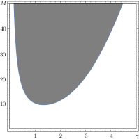
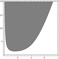
   Figure 9: The sign of the coefficient $\gamma_{2}$ as a function of $M$ and $\gamma$ for the Langevin magnetisation law (50) for rolls (left) and rectangles (right) in a ferrofluid of great depth. The shaded and white areas show the regions in which the bifurcation is respectively super- and subcritical.

This paper has no additional data. M.D.G. and J.H. collaborated equally on each aspect of this work. We declare we have no competing interests. No external funding was involved in this work.

References

[1]
Cowley MD, Rosensweig RE. 1967 The interfacial stability of a ferromagnetic
fluid. J. Fluid Mech.30, 671–688.
[2]
Twombly EE, Thomas JW. 1983 Bifurcating instability of the free surface of a
ferrofluid. SIAM J. Math. Anal.14, 736–766.
[3]
Craig W, Nicholls DP. 2000 Traveling two and three dimensional capillary
gravity water waves. SIAM J. Math. Anal.32, 323–359.
[4]
Buffoni B, Toland JF. 2003 Analytic Theory of Global Bifurcation.
Princeton, N. J.: Princeton University Press.
[5]
Sattinger DH. 1978 Group representation theory, bifurcation theory and pattern
formation. J. Func. Anal.28, 58–101.
[6]
Silber M, Knobloch E. 1988 Pattern selection in ferrofluids. Physica D30, 83–98.
[7]
Lloyd DJB, Gollwitzer C, Rehberg I, Richter R. 2015 Homoclinc snaking near the
surface instability of a polarisable fluid. J. Fluid Mech.783, 283–305.
[8]
Groves MD, Lloyd DJB, Stylianou A. 2017 Pattern formation on the free surface
of a ferrofluid: spatial dynamics and homoclinic bifurcation. Physica D350, 1–12.
[9]
Rosensweig RE. 1997 Ferrohydrodynamics.
New York: Dover.
[10]
Nicholls DP, Reitich F. 2001 A new approach to analyticity of
Dirichlet-Neumann operators. Proc. Roy. Soc. Edin. A131, 1411–1433.