Scattering of electromagnetic waves from a cone with conformal mapping: application to scanning near-field optical microscope

Abstract

We study the response of a conical metallic surface to an external electromagnetic (EM) field by representing the fields in basis functions containing integrable singularities at the tip of the cone. A fast analytical solution is obtained by the conformal mapping between the cone and a round disk. We apply our calculation to the scattering- based scanning near-field optical microscope (s-SNOM) and successfully quantify the elastic light scattering from a vibrating metallic tip over a uniform sample. We find that the field-induced charge distribution consists of localized terms at the tip and the base and an extended bulk term along the body of the cone far away from the tip. In recent s-SNOM experiments at the visible-IR range (600nm - 1$\mu m$) the fundamental is found to be much larger than the higher harmonics whereas at THz range ($100\mu m-3mm$) the fundamental becomes comparable to the higher harmonics. We find that the localized tip charge dominates the contribution to the higher harmonics and becomes bigger for the THz experiments, thus providing an intuitive understanding of the origin of the near-field signals. We demonstrate the application of our method by extracting a two-dimensional effective dielectric constant map from the s-SNOM image of a finite metallic disk, where the variation comes from the charge density induced by the EM field.

Scattering-type near-field optical microscope (s-SNOM) has made great advances over the past decade by combining the well-developed atomic force microscope (AFM) techniques with a wide range of tunable and broadband light sources. By gathering the scattered light from an AFM tip (see Fig. 1a), s-SNOM effectively probes the near-field interactions between the nanometer-sized tip apex and the sample surface, providing a spatial resolution of  10 nm, far beyond the diffraction limit of traditional opticsnov ; liu . It has shown to be extremely useful in probing phase inhomogeneities in strongly correlated electron materials1 ; 2 ; 3 ; 4 ; 5 ; 6 , polaritonic waves in 2D materials7 ; 8 ; 9 , charge concentrations in semiconductor nanostructures10 ; 11 ; 12 and molecular nano-fingerprints in organic and soft materials13 ; 14 ; 15 . The central task of quantitatively understanding the near-field signals comes down to solving a nontrivial scattering problem, of which light of frequency $\omega$ elastically scatters from a cone-shaped AFM tip oscillating vertically on the sample surface at the mechanical resonance frequency $\Omega<<\omega$ of the cantilever. Approaches from simple models such as the point dipolepd and rp modelsrp to state-of-the-art finite element calculationscst have been applied to this problem. Because of the singularity at the tip, current approaches have not been able to consistently predict the phase of the signal accurately (See Fig. 3 below). We find that the inverse extraction of the physical properties of the sample from the scattering data with current numerical approaches does not always produce unique results. It is also extremely time consuming to solve the problem without simplifying approximation and this has limited the reliable real time interpretation of the experimental data.

Here we overcame the difficulty of the singularity at the apex by using our recently developed techniquebook ; disk ; tri of representing the fields in basis functions containing integrable singularities at the tip obtained by conformal mapping between the cone and a round disk and successfully quantify the elastic light scattering from a vibrating metallic tip. We found the field-induced charge distribution to consist of a bulk term along the body of the cone far away from the tip and localized terms at the tip apex and the base. The scattering at the fundamental frequency $\omega+\Omega$ comes from both the bulk and the localized charges. The near field higher harmonics at frequencies $\omega+n\Omega$ experimentally observed is dominated by contributions from the localized charge at the tip. In recent s-SNOM experiments at the optical to mid infrared rangeliu and in the THz range ($>1mm$) the fundamental is much larger than and comparable to the higher harmonics respectively. Our calculation is in agreement with the empirical measurements where we found that the tip charge at THz frequencies is much larger than that at IR frequencies. To mimic the conical AFM tip, there have been work with different less singular tip geometries such as the sphericalpd , the spheroidal17 ; 18 ; 19 and the pear-shapedXXX . These calculations implied different induced charge distributions. Our approach provides a more systematic way to calculate the charge distributions for different experimental conditions.

Our calculation is also orders of magnitude faster than current approaches and makes this study suitable for efficiently calculating the near-field signals and tip-sample interactions over a wide range of frequencies all the way from visible to terahertz with a fast and effective theoretical treatment. We demonstrate the back-extraction of a two-dimensional map from the s-SNOM image of a finite metallic disk which effectively quantify the charge density of a finite metallic surface induced by an EM field. We now described our results in detail.

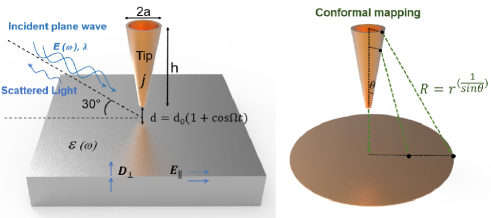
Figure 1: (a) Schematic representation of the scattering near-field setup. (b) Schematics of the conformal mapping of the cone shaped tip to a round disk.

We are interested in the current flow on a finite film caused by an external electromagnetic (EM) wave. We assume that the film is thin enough that there is no current in the direction perpendicular to it. The current density ${\bf j}$ in the presence of an external electric field ${\bf E}_{ext}$ is governed by the equation

$$\rho{\bf j+E_{em}=E}_{ext}.$$ (1)

where $\rho$ is the resistivity, ${\bf E}_{em}$ is the electromagnetic field generated by the current.We impose the boundary condition of no current flow perpendicular to the boundary of the film with a large boundary resistivity $\rho_{s}$ which we take to approach infinitybook ; disk ; tri . The total resistivity $\rho$ is a sum of this boundary term and a metal resistivity $\rho_{0}$.

Because of the singularity at the tip, it is difficult to treat the problem. Here we represent the currents and the fields not in terms of finite elements on a mesh but in terms of a complete set of orthonormal basis functions with the integrable singularity of the system built in. This rigorous approach was shown to be very efficientbook ; disk ; tri . For the simple case of an annnulus of radii $R_{1}$, $R_{2}$, the basis functions are the well known vector cylindrical functionsdisk ; tri ${\bf M}_{m}$ ${\bf N}_{m}$of angular momentum $m$ and with components $X_{r}$ and $X_{\Phi}$ (X=M, N) in the radial and the angular directions. Here we are interested in a conical film of height $h$, base radius $a$ with the cone angle $\theta=\tan^{-1}a/h$, thickness $t$ and a small flat tip of radius $b$. This geometry is closest to the experimental setup among all the theoretical models. A point on the conical surface and a point inside the annulus are characterized by the cylindrical coordinates $r$ and $\phi$ and $R$ and $\Phi$ respectively. As is illustrated in Fig. 1b, these can be mapped into each other via a conformal harmonic mapmap

$$R=r^{1/\sin\theta},\ \Phi=\phi.$$

The Jacobian of the transformation is $J=R^{2\sin\theta-2}$. We construct the basis function for this surface from the basis function of a circular annulus as

$${\bf cX}(r)=\alpha\left\{X_{r}[{\bf R}({\bf r})]{\bf e}_{1}+X_{\Phi}{\bf e}_{2}\right\}$$ (2)

where $X=M,\ N$, $\alpha=1/J^{1/2}=R/r.$ The tangent vectors on the surface of the cone are in the cylindrical basis $(r,\phi,z)$: ${\bf e}_{1}=1/(1+h^{2})^{1/2}{\bf e}_{r}-h/(1+h^{2})^{1/2}{\bf e}_{z},$ ${\bf e}_{2}={\bf e}_{\phi}$ With this choice, the new basis functions are orthonormal with the corresponding measure: $\int d^{2}r{\bf(cX_{n})^{*}\cdot cY_{m}}=\int d^{2}RJ|\alpha|^{2}{\bf X_{n}\cdot Y_{m}}=\delta_{X,Y}.$

The electromagnetic field ${\bf E}_{em}$ can be represented as ${\bf E}_{em}={\bf Z^{0}j}$ where the ”impedance” matrix $\textbf{Z}^{0}$ is just the representation of the Green’s function in this basisbook ; disk ; tri . Just as in our previous studies, when the basis functions are orthonormal, the off-diagonal elements of the impedance matrix is much less than the diagonal elements. Furthermore the magnitude of the impedance increases rapidly. These greatly facilitate the convergence of the solution and provide for a much better understanding of the physics.

In this notation, the circuit equation becomes

$${\bf Zj=E}_{ext}+{\bf E}_{s}$$ (3)

where $Z=Z^{0}+\rho_{0}$. The boundary electric field ${\bf E}_{s}$ is the product of the normal component of the current at the boundary $j_{s}$ and $\rho_{s}$, i.e. ${\bf E}_{s}={\bf j}_{s}\rho_{s}$ . They behave like Lagrange multipliers. Their values are determined from the condition that the normal boundary currents become zero. Physically, as the external field is applied, the current is stopped at the boundary and charges of surface density $\sigma_{s}$ are getting accumulated. A boundary field is generated until it reaches a value to oppose further current arriving there.

In the experiment, there is an additional sample surface of dielectric constant $\epsilon$ underneath the cone. The EM field induced charges of density $n$ on the surafce. In the presence of the plane at a distance $d=d_{0}(1-\cos\Omega t)+d_{m}$ from the tip, there will be image charges of density $n_{i}({\bf r}-2d{\bf e}_{z})=-\beta n({\bf r}),$ $\beta=(\epsilon-1)/(\epsilon+1).$ Because $d$ is much less than the wavelength the method of images is a good approximation. The total EM field now has additional contributions from the image charges. The effective impedance ${\bf Z}$ is modified. We have calculated the additional image circuit parameters and included them in the circuit equations.

Because of the image charge, the tip surface field $E_{s2}=E_{sa}+E_{sb}$ is now a sum of a field $E_{sa}$ from a surface charge of density $\sigma_{s}$ at the tip and a field $E_{sb}$ from the image charge density $-\beta\sigma_{s}$ at a distance $-d$ below the surface. From Gauss’s law $E_{sa}=\sigma_{s}/2\epsilon_{0},$ $E_{sb}\approx-\beta\sigma_{s}/\epsilon_{0}I(2d)$ where $I(x)=<E_{cz}>$ is the z Coulomb electric field from the image charge density on the tip averaged over the tip. From these equations, we get

$$\sigma_{s}=2\epsilon_{0}E_{s2}/[1-2\beta I(2d)].$$ (4)

We have calculated $I(x)$ numerically and tabulated it for a mesh of 4000 points in the region $0<x/d_{0}<2$.

Recent experiments have been carried out at IR frequency with $\lambda=10\mu m$, $h=20\mu m,$ $a=5\mu m,$ $b=10nm,$ $d_{0}=60nm,$ $t=20nm,$ $d_{m}=0.6nm$ and at THz frequency with $\lambda$ centered at $300\mu m$, $h=70\mu m,$ $a=20\mu m,$ $b=50nm,$, $d_{0}=150nm$, $d_{m}=0.6nm$. In the latter case, the tip is solid; the effective thickness of the film is thus the skin depth $\xi$. For this case $t/a\approx 0.01$ whereas for the IR case, $t/a=4\times 10^{-3}.$ We have carried out calculations for these parameters. The incoming field is at an angle of 60 degrees with respect to the surface normal. This field is nearly uniform across the tip. The coupling is thus dominated by the m=0 mode which we focus on.

We have calculated the circuit parameters ${\bf Z}$ for the m=0 modes with the basis functions $cX_{m=0}(k_{i}r)$ for up to 16 wave vectors $k_{i}$. As usual, the magnitude of $Z$ increases as $k_{i}$ is increased. This makes the problem rapidly convergent in our approach. The expansion coefficients for the current density in the basis $c{\bf N}_{0}(k_{i}r)$ are shown in Fig. (2) (right panel) where the nature of convergence of our expansion is illustrated. The current density $j=j^{c}j_{u}$ is in units of $j_{u}=E_{ext}/\rho_{u}$ where the resistivity unit is $\rho_{u}=Z_{0}\omega at/c,$ $Z_{0}$ is the resistance of the vaccum. The IR experiments were carried out at a higher normalized wave vector and thus have more intermediate components. The magnitude of the current densities as a function of the normalized position on the cone for both the IR and the THz experiments are shown in Fig. 2 (left panel).

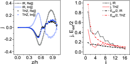
Figure 2: The magnitude of the expansion coefficient for the bulk current density $j^{c}$ (right panel) in terms of the normal modes wave vectors index $i$ and (left panel) as a function of its normalized distance from the tip for parameters for two sets of experiments in the IR and THz regime. (right panel) The magnitude of the expansion coefficient for the external field $E_{i,ext}$ in terms of $i$.

The charge density contains a bulk contribution from currents inside the cone given by $n=-i\nabla\cdot j/\omega$. Because the current density is nearly zero around the tip at $z/h\approx 0$, its spatial derivative and hence this bulk charge density is only nonzero away from the tip at a distance much larger than $d$ since $d/h<<1$. Thus this bulk charge will not contribute to near field results. The total ”bulk” charges in units of $Q_{u}=\epsilon_{0}E_{ext}a^{2}$ for the THz case [ (-0.07+0.04i) ] and the IR case [ (-0.16+0.007i) ] are comparable in magnitude.

There are additional contributions to the charge from the surface charge densities localized at the tip ($\sigma_{s2}$) and the base ($\sigma_{s1}$). $\sigma_{si}=E_{si}\sigma_{u}$ where $\sigma_{u}=2\epsilon_{0}E_{ext},$ For the IR vase, $E_{s1}/E_{ext}=0.163-0.0168i,$ $E_{s2}/E_{ext}=4.374+6.23i$. For the THz case $E_{s1}/E_{ext}=0.142+0.188i,$ $E_{s2}/E_{ext}=-28.52-14.70i.$ The magnitude of the surface charge at the tip in the THZ case is five times bigger than that for the IR experiments. This comes about because the wavelength of the external field is much closer to the size of the cone for the THZ experiments, $E_{i,ext}$ is dominated by the component with i=1, as is illustrated in Fig. 2.

We next look at the scattered field $S_{n}$ at the modulated frequencies $\omega+n\Omega$ from the moving bulk and surface charges. The scattered fields at a distance r from the tip are proportional to the vector potential given byJackson ${\bf A}(r)=i\omega\mu_{0}e^{ikr}\int d{\bf r^{\prime}}{\bf j}(r^{\prime})/r.$ The total current density of the vibrating tip is a sum of a current induced by the incoming field and a current $j_{d}=n\partial_{t}d$ from the induced charge $n$ and the vibration of the tip $\partial_{t}d$. $n$ contains both bulk and boundary charge contributions. The ”bulk” charges contribute mainly to the fundamental with n=1. The contributions to the higher harmonics with $n>1$ is dominated by near field contributions when the tip is close to the surface and comes mainly from the localized charge at the tip. The radiation electric field $S_{n}$ is proportional to the Fourier transform at frequency $\omega+n\Omega$ of the contributions $j_{dl}$ to $j_{d}$ from the localized charges at the tip. From Eq. (4) we get

$$E\propto e^{i\omega t}(1+\beta)\cos(\Omega t)/[1-2\beta I(d)].$$ (5)

As a test, we have calculated the amplitude $S_{2}$ and its phase as a function of frequency using as input dielectric constants corresponding to a uniform surface of $SiO_{2}$. The experimental result together with ours are shown in the left panel Fig. (3). The overall magnitude of the amplitudes and the baseline for the phase depend on the experimental geometry and thus are the two adjustable parameters. The agreement is very good. For comparison, results obtained with commonly used simple tip modelling as well as CST simulation with a similar tip geometry are shown in the right panel. The agreement with the experimental phase is not as accurate.

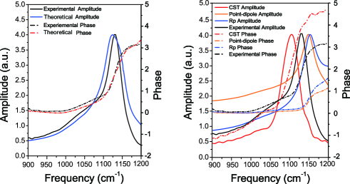
Figure 3: Left Panel: Our theoretical and experimental results for the amplitude $S_{2}$ and the phase $\phi_{2}$ of uniform $SiO_{2}$ as a function of frequency. Right Panel: $S_{2}$ and $\phi_{2}$ calculated with the Rp model, the point-dipole model, and with the CST numerical solver, together with the experimental result.

The fundamental is comparable and much larger than the higher harmonics respectively in recent experiments carried out at the THz and the IR frequencies. The localized tip charge dominates the contribution to the higher harmonics and becomes much bigger for the THz experiments, providing an intuitive understanding of the origin of the near-field signals.

We close with an example of the inverse problem of extracting the physical properties from the measuredexpt higher harmonics response for a gold disk of diameter approximately 1.3 $\mu m$ and thickness $\approx 50nm$. We calculated a table of $S_{3}$ and $\phi_{3}$ as functions of $-0.1<Re[\beta]<1.4,$ $-0.5<Im[\beta]<0.5$ from eq. (5) for a mesh of 6400 grid points .This takes 2.7 sec with a conventional Intel processor. For a pixel at position ${\bf r}$, we go through the entries in our table and identify $\beta({\bf r})$ as the one such that $|S_{3}(\beta({\bf r}))-S_{3}^{expt}({\bf r})|+|\phi_{3}(\beta({\bf r}))-\phi_{3}^{expt}({\bf r})|$ is minimized. This calculation takes 0.77 s for a data set of $128\times 128$ pixels.

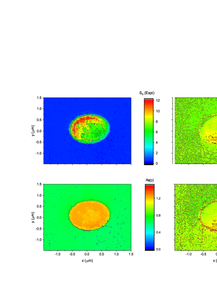
Figure 4: Top Panels: The experimental amplitude and phase of the third harmonics as a function of position on the disk. Bottom Panels: The extracted values of $\beta$.

Two dimensional plots of $\beta$, $S_{3}$ and $\phi_{3}$ are shown in Fig. 4. Even though the material exhibits the same intrinsic $\epsilon$ independent of position, there is a variation in the extracted $\beta$ from the average value. We believe that is due to charge densities on the disk induced by the EM field . More precisely, $\beta$ is determined from the condition that the change of the perpendicular component of the displacement field $D_{\perp}$ at the disk-air interface is equal to the surface charge denisty $\sigma_{disk}$: $\Delta D_{\perp}=\sigma_{disk}.$ Our study of the EM scattering on disksdisk suggests that there is an edge electric field and its associated charge at the perimeter of the disk. The variation of the physical quantities is indeed dominated by changes at the perimeter, in agreement with our expectation.

To get a more quantitative picture of our results, we plot the physical quantities as a function of the position across a diameter of the disk along the direction of the EM field are shown in Fig. 5. The experimental amplitude and phase of the third harmonics (top panels) are well reproduced. This substantiates the calculation reported in this paper. The extracted $\beta$ are shown in the bottom panels. We found that $Re[\beta]\approx 1.2$ (0), $Im[\beta]\approx 0.07$ (0) inside (outside) the disk. This technique may also be a new tool for mapping of the changes induced by external fields. The detailed analysis of this will be discussed in a separate paper.

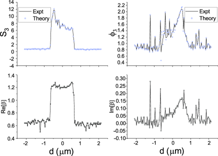
Figure 5: Top Panels: The experimental amplitude and phase of the third harmonics together with the theoretical result for a metallic disk.Bottom Panels: The extracted values of $\beta.$ These are as a function of position across a diameter of the disk.

In conclusion, we study the elastic scattering of an EM wave by a conical metallic surface via representing the fields on the surface in basis functions containing the integrable singularities at the tip. We apply our calculation to s-SNOM and found good agreement with experimental results from a vibrating metallic tip over a uniform sample. We found the field-induced charge distribution consists of a bulk term along the body of the cone and localized terms at the tip apex and the base. The bulk charge is far away from the tip and contributes little to the near-field higher harmonics in the scattered field. The localized boundary charges at the tip apex contribute to the near-field signal and correspond to the charge accumulation effects previously discussed in pn junctions and on the surface of capacitor plates in AC experimentskittel ; ac ; hebard . In these treatments, the additional physics of the diffusion of the electrons are included and a finite width in the localized charge distribution of the order of the screening length is found. This localized boundary charge provides new insight into the physics of the scattering problem, which can be related to the distinct $S_{1}/S_{2}$ ratio found in recent experiments at IR and THz frequencies. In addition, we also demonstrate the application of our technique by extracting a two-dimensional effective dielectric constant map of a finite plasmonic metallic disk from experimental data, which is non-uniform due to the induced charge density distribution under the illumination of EM field. Our calculations of the scattering signal and the back-extraction process are more realistic and much faster compared to the prevailing analytical and numerical approaches. Future studies will include the calculation of near-field scattering signal of nonuniform samples.

References

- (1) Novotny, L. Prog. Opt. 2008, 50, 137–184.
- (2) Liu, M.; Sternbach, A. J.; Basov, D. N. Reports Prog. Phys. 2017, 80, 14501.
- (3) M. M. Qazilbash, M. Brehm, B.-G. Chae, P.-C. Ho, G. O. Andreev, B.-J. Kim, S. J. Yun, A. V Balatsky, M. B. Maple, F. Keilmann, H.-T. Kim, and D. N. Basov, Science 318, 1750 (2007)
- (4) S. A. Dönges, O. Khatib, B. T. O’Callahan, J. M. Atkin, J. H. Park, D. Cobden, and M. B. Raschke, Nano Lett. 16, 3029 (2016).
- (5) M. A. Huber, M. Plankl, M. Eisele, R. E. Marvel, F. Sandner, T. Korn, C. Schüller, R. F. Haglund, R. Huber, and T. L. Cocker, Nano Lett. 16, 1421 (2016).
- (6) M. K. Liu, M. Wagner, E. Abreu, S. Kittiwatanakul, A. McLeod, Z. Fei, M. Goldflam, S. Dai, M. M. Fogler, J. Lu, S. A. Wolf, R. D. Averitt, and D. N. Basov, Phys. Rev. Lett. 111, 96602 (2013).
- (7) M. Liu, A. J. Sternbach, and D. N. Basov, Reports Prog. Phys. 80, 14501 (2017).
- (8) A. S. McLeod, E. van Heumen, J. G. Ramirez, S. Wang, T. Saerbeck, S. Guenon, M. Goldflam, L. Anderegg, P. Kelly, A. Mueller, M. K. Liu, I. K. Schuller, and D. N. Basov, Nat. Phys. 13, 80 (2017).
- (9) Z. Fei, A. S. Rodin, G. O. Andreev, W. Bao, A. S. McLeod, M. Wagner, L. M. Zhang, Z. Zhao, M. Thiemens, G. Dominguez, M. M. Fogler, A. H. Castro Neto, C. N. Lau, F. Keilmann, and D. N. Basov, Nature 487, 82 (2012).
- (10) J. Chen, M. Badioli, P. Alonso-González, S. Thongrattanasiri, F. Huth, J. Osmond, M. Spasenović, A. Centeno, A. Pesquera, P. Godignon, A. Zurutuza Elorza, N. Camara, F. J. G. de Abajo, R. Hillenbrand, and F. H. L. Koppens, Nature 487, 77 (2012).
- (11) S. Dai, Q. Ma, M. K. Liu, T. Andersen, Z. Fei, M. D. Goldflam, M. Wagner, K. Watanabe, T. Taniguchi, M. Thiemens, F. Keilmann, G. C. a. M. Janssen, S.-E. Zhu, P. Jarillo-Herrero, M. M. Fogler, and D. N. Basov, Nat. Nanotechnol. 1 (2015).
- (12) F. Buersgens, R. Kersting, and H. T. Chen, Appl. Phys. Lett. 88, 88 (2006).
- (13) K. Moon, H. Park, J. Kim, Y. Do, S. Lee, G. Lee, H. Kang, and H. Han, Nano Lett. 15, 549 (2015).
- (14) A. J. Huber, F. Keilmann, J. Wittborn, J. Aizpurua, and R. Hillenbrand, Nano Lett. 8, 3766 (2008).
- (15) H. A. Bechtel, E. A. Muller, R. L. Olmon, M. C. Martin, and M. B. Raschke, Proc. Natl. Acad. Sci. U. S. A. 111, 7191 (2014).
- (16) I. Amenabar, S. Poly, M. Goikoetxea, W. Nuansing, P. Lasch, and R. Hillenbrand, Nat. Commun. 8, 14402 (2017).
- (17) N. Qin, S. Zhang, J. Jiang, S. G. Corder, Z. Qian, Z. Zhou, W. Lee, K. Liu, X. Wang, X. Li, Z. Shi, Y. Mao, H. A. Bechtel, M. C. Martin, X. Xia, B. Marelli, D. L. Kaplan, F. G. Omenetto, M. Liu, and T. H. Tao, Nat. Commun. 7, 13079 (2016).
- (18) F. Keilmann and R. Hillenbrand, Philos. Trans. A. Math. Phys. Eng. Sci. 362, 787 (2004).
- (19) S. Dai, Z. Fei, Q. Ma, A. S. Rodin, M. Wagner, A. S. McLeod, M. K. Liu, W. Gannett, W. Regan, K. Watanabe, T. Taniguchi, M. Thiemens, G. Dominguez, A. H. C. Neto, A. Zettl, F. Keilmann, P. Jarillo-Herrero, M. M. Fogler, and D. N. Basov, Science (80-. ). 343, 1125 (2014).
- (20) Numerical calculations with the commerical software ”COMSOL” was reported by many authors but we could not find any published result for the phase. We have carried out calculations with a comparable commerical oftware ”CST Studio” and the amplitude and the phase is reported below.
- (21) A. Cvitkovic, N. Ocelic, and R. Hillenbrand, Opt. Express 15, 8550 (2007).
- (22) A. S. McLeod, P. Kelly, M. D. Goldflam, Z. Gainsforth, A. J. Westphal, G. Dominguez, M. H. Thiemens, M. M. Fogler, and D. N. Basov, Phys. Rev. B - Condens. Matter Mater. Phys. 90, 085136 (2014).
- (23) B. Hauer, A. P. Engelhardt, and T. Taubner, Opt. Express 20, 13173 (2012).
- (24) B.-Y. Jiang, L. M. Zhang, A. H. Castro Neto, D. N. Basov and M. M. Fogler JOURNAL OF APPLIED PHYSICS 119, 054305 (2016).
- (25) S. T. Chui and Lei Zhou, ” Electromagnetic behaviour of metallic wire structures”, Springer, (2013).
- (26) S. T. Chui, J. J. Du and S. T. Yau, Phys. Rev. E 90, 053202 (2014).
- (27) Chui, S. T.; Wang, Shubo; Chan, C. T. PHYSICAL REVIEW E93, 033302 (2016).
- (28) Lambert, Johann Heinrich (1772) ”Notes and Comments on the Composition of Terrestrial and Celestial Maps” (Translated and Introduced by W. R. Tobler, 1972. ESRI Press. ISBN 978-1-58948-281-4); S.T. Chui, unpublished.
- (29) J. D. Jackson, Eq. 9.13 in ”Classical Electrodynamics”, Wiley.
- (30) X. Chen and M. Liu, unpublished.
- (31) C. KIttel, Chap. 8, ”Introduction to Solid State Physics”
- (32) S. T. Chui and L. Hu, Appl. Phys. Lett. 80, 273 (2002).
- (33) A. F. Hebard, S. A. Ajuria, and R. H. Eick, Appl. Phys. Lett. 51, 1349 (1987͒).