Dual Free Adaptive Minibatch SDCA
for Empirical Risk Minimization

Abstract

In this paper we develop an adaptive dual free Stochastic Dual Coordinate Ascent (adfSDCA) algorithm for regularized empirical risk minimization problems. This is motivated by the recent work on dual free SDCA of Shalev-Shwartz (2016). The novelty of our approach is that the coordinates to update at each iteration are selected non-uniformly from an adaptive probability distribution, and this extends the previously mentioned work which only allowed for a uniform selection of “dual” coordinates from a fixed probability distribution.

We describe an efficient iterative procedure for generating the non-uniform samples, where the scheme selects the coordinate with the greatest potential to decrease the sub-optimality of the current iterate. We also propose a heuristic variant of adfSDCA that is more aggressive than the standard approach. Furthermore, in order to utilize multi-core machines we consider a mini-batch adfSDCA algorithm and develop complexity results that guarantee the algorithm’s convergence. The work is concluded with several numerical experiments to demonstrate the practical benefits of the proposed approach.

1 Keywords:

SDCA, Importance Sampling, Non-uniform Sampling, Mini-batch, Adaptive

2 Introduction

In this work we study the $\ell_{2}$-regularized Empirical Risk Minimization (ERM) problem, which is widely used in the field of machine learning. The problem can be stated as follows. Given training examples $(x_{1},y_{1}),\dots,(x_{n},y_{n})\in\mathbb{R}^{d}\times\mathbb{R}$, loss functions $\phi_{1},\dots,\phi_{n}:\mathbb{R}\rightarrow\mathbb{R}$ and a regularization parameter $\lambda>0$, $\ell_{2}$-regularized ERM is an optimization problem of the form

$$\min_{w\in\mathbb{R}^{d}}P(w):=\frac{1}{n}\sum_{i=1}^{n}\phi_{i}(w^{T}x_{i})+\frac{\lambda}{2}\|w\|^{2},$$ (P)

where the first term in the objective function is a data fitting term and the second is a regularization term that prevents over-fitting.

Many algorithms have been proposed to solve problem (P) over the past few years, including SGD, Shalev-Shwartz et al. (2011), SVRG and S2GD, Johnson and Zhang (2013); Nitanda (2014); Konečný et al. (2016) and SAG/SAGA, Schmidt et al. (2017); Defazio et al. (2014); Roux et al. (2012). However, another very popular approach to solving $\ell_{2}$-regularized ERM problems is to consider the following dual formulation

$$\max_{\alpha\in\mathbb{R}^{n}}D(\alpha):=-\frac{1}{n}\sum_{i=1}^{n}\phi^{*}_{i}(-\alpha_{i})-\frac{\lambda}{2}\|\frac{1}{\lambda n}X^{T}\alpha\|^{2},$$ (D)

where $X^{T}=[x_{1},\dots,x_{n}]\in\mathbb{R}^{d\times n}$ is the data matrix and $\phi_{i}^{*}$ denotes the convex conjugate of $\phi_{i}$. The structure of the dual formulation (D) makes it well suited to a multicore or distributed computational setting, and several algorithms have been developed to take advantage of this including Hsieh et al. (2008) Takáč et al. (2013); Jaggi et al. (2014); Ma et al. (2015); Takáč et al. (2015); Qu et al. (2015); Csiba et al. (2015); Zhang and Xiao (2015).

One of the most popular methods for solving (D) is Stochastic Dual Coordinate Ascent (SDCA). The algorithm proceeds as follows. At iteration $t$ of SDCA a coordinate $i\in\{1,\dots,n\}$ is chosen uniformly at random and the current iterate $\alpha^{(t)}$ is updated to $\alpha^{(t+1)}:=\alpha^{(t)}+\delta^{*}e_{i}$, where $\delta^{*}=\arg\max_{\delta\in\mathbb{R}}D(\alpha^{(t)}+\delta e_{i})$. Much research has focused on analysing the theoretical complexity of SDCA under various assumptions imposed on the functions $\phi_{i}^{*}$, including the pioneering work of Nesterov in Nesterov (2012) and others including Richtárik and Takáč (2014); Tappenden et al. (2017); Necoara and Clipici (2013, 2016); Liu and Wright (2015); Takáč et al. (2015, 2013).

A modification that has led to improvements in the practical performance of SDCA is the use of importance sampling when selecting the coordinate to update. That is, rather than using uniform probabilities, instead coordinate $i$ is sampled with an arbitrary probability $p_{i}$, see for example Zhao and Zhang (2015); Csiba et al. (2015).

In many cases algorithms that employ non-uniform coordinate sampling outperform naïve uniform selection, and in some cases help to decrease the number of iterations needed to achieve a desired accuracy by several fold.

Notation and Assumptions. In this work we use the notation $[n]\stackrel{{\scriptstyle\text{def}}}{{=}}\{1,\dots,n\}$, as well as the following assumption. For all $i\in[n]$, the loss function $\phi_{i}$ is $\tilde{L}_{i}$-smooth with $\tilde{L}_{i}>0$, i.e., for any given $\beta,\delta\in\mathbb{R}$, we have

$$|\phi_{i}^{\prime}(\beta)-\phi_{i}^{\prime}(\beta+\delta)|\leq\tilde{L}_{i}|\delta|.$$ (1)

In addition, it is simple to observe that the function $\phi_{i}(x_{i}^{T}\cdot):\mathbb{R}^{d}\to\mathbb{R}$ is $L_{i}$ smooth, i.e., $\forall w,\bar{w}\in\mathbb{R}^{d}$ and for all $i\in[n]$ there exists a constant $L_{i}\leq\|x_{i}\|^{2}\tilde{L}_{i}$ such that

$$\|\nabla\phi_{i}(x_{i}^{T}w)-\nabla\phi_{i}(x_{i}^{T}\bar{w})\|\leq L_{i}\|w-\bar{w}\|.$$ (2)

We will use the notation

$$L=\max_{1\leq i\leq n}L_{i},\qquad\text{and}\qquad\tilde{L}=\max_{1\leq i\leq n}\tilde{L}_{i}.$$ (3)

Throughout this work we let $\mathbb{R}_{+}$ denote the set of nonnegative real numbers and we let $\mathbb{R}_{+}^{n}$ denote the set of $n$-dimensional vectors with all components being real and nonnegative.

2.1 Contributions

In this section the main contributions of this paper are summarized (not in order of significance).

Adaptive SDCA. We modify the dual free SDCA algorithm proposed in Shalev-Shwartz (2015) to allow for the adaptive adjustment of probabilities and a non-uniform selection of coordinates. Note that the method is dual free, and hence in contrast to classical SDCA, where the update is defined by maximizing the dual objective (D), here we define the update slightly differently (see Section 3 for details).

Allowing non-uniform selection of coordinates from an adaptive probability distribution leads to improvements in practical performance and the algorithm achieves a better complexity bound than in Shalev-Shwartz (2015). We show that the error after $T$ iterations is decreased by factor of $\prod_{t=1}^{T}(1-\theta^{(t)})\geq(1-\theta^{*})^{T}$ on average, where $\theta^{*}$ is an uniformly lower bound for all $\theta^{(t)}$. Here $1-\theta^{(t)}\in(0,1)$ is a parameter that depends on the current iterate $\alpha^{(t)}$ and the nonuniform probability distribution. By changing the coordinate selection strategy from uniform selection to adaptive, each $1-\theta^{(t)}$ becomes smaller, which leads to an improvement in the convergence rate.

Non-uniform sampling procedure. Rather than using a uniform sampling of coordinates, which is the commonly used approach, here we propose the use of non-uniform sampling from an adaptive probability distribution. With this novel sampling strategy, we are able to generate non-uniform non-overlapping and proper (see Section 6) samplings for arbitrary marginal distributions under only one mild assumptions. Indeed, we show that without the assumption, there is no such non-uniform sampling strategy. We also extend our sampling strategy to allow the selection of mini-batches.

Better convergence and complexity results. By utilizing an adaptive probabilities strategy, we can derive complexity results for our new algorithm that, for the case when every loss function is convex, depend only on the average of the Lipschitz constants $L_{i}$. This improves upon the complexity theory developed in Shalev-Shwartz (2015) (which uses a uniform sampling) and Csiba and Richtárik (2015) (which uses an arbitrary but fixed probability distribution), because the results in those works depend on the maximum Lipschitz constant. Furthermore, even though adaptive probabilities are used here, we are still able to retain the very nice feature of the work in Shalev-Shwartz (2015), and show that the variance of the update naturally goes to zero as the iterates converge to the optimum without any additional computational effort or storage costs. Our adaptive probabilities SDCA method also comes with an improved bound on the variance of the update in terms of the sub-optimality of the current iterate.

Practical aggressive variant. Following from the work of Csiba et al. (2015), we propose an efficient heuristic variant of adfSDCA. For adfSDCA the adaptive probabilities must be computed at every iteration (i.e., once a single coordinate has been selected), which can be computationally expensive. However, for our heuristic adfSDCA variant the (exact/true) adaptive probabilities are only computed once at the beginning of each epoch (where an epoch is one pass over the data/$n$ coordinate updates), and during that epoch, once a coordinate has been selected we simply reduce the probability associated with that coordinate so it is not selected again during that epoch. Intuitively this is reasonable because, after a coordinate has been updated the dual residue associated with that coordinate decreases and thus the probability of choosing this coordinate should also reduce. We show that in practice this heuristic adfSDCA variant converges and the computational effort required by this algorithm is lower than adfSDCA (see Sections 5 and 7).

Mini-batch variant. We extend the (serial) adfSDCA algorithm to incorporate a mini-batch scheme. The motivation for this approach is that there is a computational cost associated with generating the adaptive probabilities, so it is important to utilize them effectively. We develop a non-uniform mini-batch strategy that allows us to update multiple coordinates in one iteration, and the coordinates that are selected have high potential to decrease the sub-optimality of the current iterate. Further, we make use of ESO framework (Expected Separable Overapproximation) (see for example Richtárik and Takáč (2012), Qu et al. (2015)) and present theoretical complexity results for mini-batch adfSDCA. In particular, for mini-batch adfSDCA used with batchsize $b$, we derive the optimal probabilities to use at each iteration, as well as the best step-size to use to guarantee speedup.

2.2 Outline

This paper is organized as follows. In Section 3 we introduce our new Adaptive Dual Free SDCA algorithm (adfSDCA), and highlight its connection with a reduced variance SGD method. In Section 4 we provide theoretical convergence guarantees for adfSDCA in the case when all loss functions $\phi_{i}(\cdot)$ are convex, and also in the case when individual loss functions are allowed to be nonconvex but the average loss functions $\sum_{i=1}^{n}\phi_{i}(\cdot)$ is convex. Section 5 introduces a practical heuristic version of adfSDCA, and in Section 6 we present a mini-batch adfSDCA algorithm and provide convergence guarantees for that method. Finally, we present the results of our numerical experiments in Section 7. Note that the proofs for all the theoretical results developed in this work are left to the appendix.

3 The Adaptive Dual Free SDCA Algorithm

In this section we describe the Adaptive Dual Free SDCA (adfSDCA) algorithm, which is motivated by the dual free SDCA algorithm proposed by Shalev-Shwartz (2015). Note that in dual free SDCA two sequences of primal and dual iterates, $\{w^{(t)}\}_{t=0}^{\infty}$ and $\{\alpha^{(t)}\}_{t=0}^{\infty}$ respectively, are maintained. At every iteration of that algorithm, the variable updates are computed in such a way that the well known primal-dual relational mapping holds; for every iteration $t$:

$$w^{(t)}=\frac{1}{\lambda n}{\sum}_{i=1}^{n}\alpha_{i}^{(t)}x_{i}.$$ (4)

The dual residue is defined as follows.

Definition 1 (Dual residue, Csiba et al. (2015)).

The dual residue $\kappa^{(t)}=(\kappa^{(t)}_{1},\dots,\kappa^{(t)}_{n})^{T}\in\mathbb{R}^{n}$ associated with $(w^{(t)},\alpha^{(t)})$ is given by:

$$\kappa_{i}^{(t)}\stackrel{{\scriptstyle\text{def}}}{{=}}\alpha_{i}^{(t)}+\phi^{\prime}_{i}(x_{i}^{T}w^{(t)}).$$ (5)

The Adaptive Dual Free SDCA algorithm is outlined in Algorithm 1 and is described briefly now; a more detailed description (including a discussion of coordinate selection and how to generate appropriate selection rules) will follow. An initial solution $\alpha^{(0)}$ is chosen, and then $w^{(0)}$ is defined via (4). In each iteration of Algorithm 1 the dual residue $\kappa^{(t)}$ is computed via (5), and this is used to generate a probability distribution $p^{(t)}$. Next, a coordinate $i\in[n]$ is selected (sampled) according to the generated probability distribution and a step is taken by updating the $i$th coordinate of $\alpha$ via

$$\alpha_{i}^{(t+1)}=\alpha_{i}^{(t)}-\theta^{(t)}(p_{i}^{(t)})^{-1}\kappa^{(t)}_{i}.$$ (6)

Finally, the vector $w$ is also updated

$$w^{(t+1)}=w^{(t)}-\theta^{(t)}(n\lambda p_{i}^{(t)})^{-1}\kappa^{(t)}_{i}x_{i},$$ (7)

and the process is repeated. Note that the updates to $\alpha$ and $w$ using the formulas (6) and (7) ensure that the equality (4) is preserved.

Also note that the updates in (6) and (7) involve a step size parameter $\theta^{(t)}$, which will play an important role in our complexity results. The step size $\theta^{(t)}$ should be large so that good progress can be made, but it must also be small enough to ensure that the algorithm is guaranteed to converge. Indeed, in Section 4.1 we will see that the choice of $\theta^{(t)}$ depends on the choice of probabilities used at iteration $t$, which in turn depend upon a particular function that is related to the suboptimality at iteration $t$.

Algorithm 1 Adaptive Dual Free SDCA (adfSDCA)

1:  Input: Data: $\{x_{i},\phi_{i}\}_{i=1}^{n}$

2:  Initialization: Choose $\alpha^{(0)}\in\mathbb{R}^{n}$

3:  Set $w^{(0)}=\tfrac{1}{\lambda n}\sum_{i=1}^{n}\alpha_{i}^{(0)}x_{i}$

4:  for $t=0,1,2,\dots$ do

5:     Calculate dual residual $\kappa^{(t)}_{i}=\phi^{\prime}_{i}(x_{i}^{T}w^{(t)})+\alpha^{(t)}_{i}$, for all $i\in[n]$

6:     Generate adaptive probability distribution $p^{(t)}\sim\kappa^{(t)}$

7:     Sample coordinate $i$ according to $p^{(t)}$

8:     Set step-size $\theta^{(t)}\in(0,1)$ as in (18)

9:     Update: $\alpha_{i}^{(t+1)}=\alpha_{i}^{(t)}-\theta^{(t)}(p_{i}^{(t)})^{-1}\kappa^{(t)}_{i}$

10:     Update: $w^{(t+1)}=w^{(t)}-\theta^{(t)}(n\lambda p_{i}^{(t)})^{-1}\kappa^{(t)}_{i}x_{i}$

11:  end for

The dual residue $\kappa^{(t)}$ is informative and provides a useful way of monitoring suboptimality of the current solution $(w^{(t)},\alpha^{(t)})$. In particular, note that if $\kappa_{i}=0$ for some coordinate $i$, then by (5) $\alpha_{i}=-\phi^{\prime}_{i}(w^{T}x_{i})$, and substituting $\kappa_{i}$ into (6) and (7) shows that $\alpha_{i}^{(t+1)}\leftarrow\alpha_{i}^{(t)}$ and $w_{i}^{(t+1)}\leftarrow w^{(t)}$, i.e., $\alpha$ and $w$ remain unchanged in that iteration. On the other hand, a large value of $|\kappa_{i}|$ (at some iteration $t$) indicates that a large step will be taken, which is anticipated to lead to good progress in terms of improvement in sub-optimality of current solution.

The probability distributions used in Algorithm 1 adhere to the following definition.

Definition 2.

(Coherence, Csiba et al. (2015)) Probability vector $p\in\mathbb{R}^{n}$ is coherent with dual residue $\kappa\in\mathbb{R}^{n}$ if for any index $i$ in the support set of $\kappa$, denoted by $I_{\kappa}:=\{i\in[n]:\kappa_{i}\neq 0\}$, we have $p_{i}>0$. When $i\notin I_{\kappa}$ then $p_{i}=0$. We use $p\sim\kappa$ to represent this coherent relation.

3.1 Adaptive dual free SDCA as a reduced variance SGD method.

Reduced variance SGD methods have became very popular in the past few years, see for example Konečný and Richtárik (2017); Johnson and Zhang (2013); Roux et al. (2012); Defazio et al. (2014). It is show in Shalev-Shwartz (2015) that uniform dual free SDCA is an instance of a reduced variance SGD algorithm (the variance of the stochastic gradient can be bounded by some measure of sub-optimality of the current iterate) and a similar result applies to adfSDCA in Algorithm 1. In particular, note that conditioned on $w^{(t-1)}$, we have

$$\mathbf{E}[w^{(t)}|\alpha^{(t-1)}] \overset{\eqref{wupdate}}{=}w^{(t-1)}-\frac{\theta^{(t-1)}}{\lambda}\sum_{i=1}^{n}\frac{p_{i}}{np_{i}}\left(\big{(}\nabla\phi_{i}(x_{i}^{T}w^{(t-1)})+\alpha_{i}^{(t-1)}\big{)}x_{i}\right)$$

$$\overset{\eqref{eq:walphaPDmap}}{=}w^{(t-1)}-\frac{\theta^{(t-1)}}{\lambda}\Big{(}\nabla\Big{(}\frac{1}{n}\sum_{i=1}^{n}\phi_{i}(x_{i}^{T}w^{(t-1)})\Big{)}+\lambda w^{(t-1)}\Big{)}$$

$$\overset{\eqref{Prob: L2EMR}}{=}w^{(t-1)}-\frac{\theta^{(t-1)}}{\lambda}\nabla P(w^{(t-1)}).$$ (8)

Combining (7) and (8) gives

$$\mathbf{E}\left[\frac{1}{np_{i}}\kappa_{i}^{(t)}x_{i}|\alpha^{(t-1)}\right]=\nabla P(w^{(t)}),$$ (9)

which implies that $\displaystyle\tfrac{1}{np_{i}}\kappa_{i}^{(t)}x_{i}$ is an unbiased estimator of $\nabla P(w^{(t)})$. Therefore, Algorithm 1 is eventually a variant of the Stochastic Gradient Descent method. However, we can prove (see later) that the variance of the update goes to zero as the iterates converge to an optimum, which is not true for vanilla Stochastic Gradient Descent.

4 Convergence Analysis

In this section we state the main convergence results for adfSDCA (Algorithm 1). The analysis is broken into two cases. In the first case it is assumed that each of the loss functions $\phi_{i}$ is convex. In the second case this assumption is relaxed slightly and it is only assumed that the average of the $\phi_{i}$’s is convex, i.e., individual functions $\phi_{i}(\cdot)$ for some (several) $i\in[n]$ are allowed to be nonconvex, as long as $\frac{1}{n}\sum_{j=1}^{n}\phi_{j}(\cdot)$ is convex. The proofs for all the results in this section can be found in the Appendix.

4.1 Case I: All loss functions are convex

Here we assume that $\phi_{i}$ is convex for all $i\in[n]$. Define the following parameter

$$\gamma\stackrel{{\scriptstyle\text{def}}}{{=}}\lambda\tilde{L},$$ (10)

where $\tilde{L}$ is given in (3). It will also be convenient to define the following potential function. For all iterations $t\geq 0$,

$$D^{(t)}\stackrel{{\scriptstyle\text{def}}}{{=}}\tfrac{1}{n}\|\alpha^{(t)}-\alpha^{*}\|^{2}+\gamma\|w^{(t)}-w^{*}\|^{2}.$$ (11)

The potential function (11) plays a central role in the convergence theory presented in this work. It measures the distance from the optimum in both the primal and (pseudo) dual variables. Thus, our algorithm will generate iterates that reduce this suboptimality and therefore push the potential function toward zero.

Also define

$$v_{i}\stackrel{{\scriptstyle\text{def}}}{{=}}\|x_{i}\|^{2}\text{ for all }i\in[n].$$ (12)

We have the following result.

Lemma 1.

Let $\tilde{L}$, $\kappa_{i}^{(t)}$, $\gamma$, $D^{(t)}$, and $v_{i}$ be as defined in (3), (5), (10), (11) and (12), respectively. Suppose that $\phi_{i}$ is $\tilde{L}$-smooth and convex for all $i\in[n]$ and let $\theta\in(0,1)$. Then at every iteration $t\geq 0$ of Algorithm 1, a probability distribution $p^{(t)}$ that satisfies Definition 2 is generated and

$$\mathbf{E}\big{[}D^{(t+1)}|\alpha^{(t)}\big{]}-(1-\theta)D^{(t)}\leq\sum_{i=1}^{n}\left(-\frac{\theta}{n}\bigg{(}1-\frac{\theta}{p_{i}^{(t)}}\bigg{)}+\frac{\theta^{2}v_{i}\gamma}{n^{2}\lambda^{2}p_{i}^{(t)}}\right)(\kappa_{i}^{(t)})^{2}.$$ (13)

Note that if the right hand side of (13) is negative, then the potential function decreases (in expectation) in iteration $t$:

$$\mathbf{E}\big{[}D^{(t+1)}|\alpha^{(t)}\big{]}\leq(1-\theta)D^{(t)}.$$ (14)

The purpose of Algorithm 1 is to generate iterates $(w^{(t)},\alpha^{(t)})$ such that the above holds. To guarantee negativity of the right hand term in (13), or equivalently, to ensure that (14) holds, consider the parameter $\theta$. Specifically, any $\theta$ that is less than the function $\Theta(\cdot,\cdot):\mathbb{R}_{+}^{n}\times\mathbb{R}_{+}^{n}\rightarrow\mathbb{R}$ defined as

$$\Theta(\kappa,p)\stackrel{{\scriptstyle\text{def}}}{{=}}\frac{n\lambda^{2}\sum_{i\in I_{\kappa}}\kappa_{i}^{2}}{\sum_{i\in I_{\kappa}}(n\lambda^{2}+v_{i}\gamma)p_{i}^{-1}\kappa_{i}^{2}},$$ (15)

will ensure negativity of (13). Moreover, the larger the value of $\theta$, the better progress Algorithm 1 will make in terms of the reduction in $D^{(t)}$. The function $\Theta$ depends on the dual residue $\kappa$ and the probability distribution $p$. Maximizing this function w.r.t. $p$ will ensure that the largest possible value of $\theta$ can be used in Algorithm 1. Thus, we consider the following optimization problem:

$$\max_{p\in\mathbb{R}^{n}_{+},\sum_{i\in I_{\kappa}}p_{i}=1}\quad \Theta(\kappa,p).$$ (16)

One may naturally be wary of the additional computational cost incurred by solving the optimization problem in (16) at every iteration. Fortunately, it turns out that there is an (inexpensive) closed form solution, as shown by the following Lemma.

Lemma 2.

Let $\Theta(\kappa,p)$ be defined in (15). The optimal solution $p^{*}(\kappa)$ of (16) is

$$p^{*}_{i}(\kappa)=\frac{\sqrt{v_{i}\gamma+n\lambda^{2}}|\kappa_{i}|}{\sum_{j\in I_{\kappa}}\sqrt{v_{j}\gamma+n\lambda^{2}}|\kappa_{j}|},\qquad\text{for all }\;i=1,\dots,n.$$ (17)

The corresponding $\theta$ by using the optimal solution $p^{*}$ is

$$\theta=\Theta(\kappa,p^{*})=\frac{n\lambda^{2}\sum_{i\in I_{\kappa}}\kappa_{i}^{2}}{(\sum_{i\in I_{\kappa}}\sqrt{v_{i}\gamma+n\lambda^{2}}|\kappa_{i}|)^{2}}.$$ (18)

Proof.

This can be verified by deriving the KKT conditions of the optimization problem in (16). The details are moved to Appendix for brevity. ∎

The results in Csiba and Richtárik (2015) are weaker because they require a fixed sampling distribution $p$ throughout all iterations. Here we allow adaptive sampling probabilities as in (17), which enables the algorithm to utilize the data information more effectively, and hence we have a better convergence rate. Furthermore, the optimal probabilities found in Csiba et al. (2015) can be only applied to a quadratic loss function, whereas our results are more general because the optimal probabilities in (17) can used whenever the loss functions are convex, or when individual loss functions are non-convex but the average of the loss functions is convex.

Before proceeding with the convergence theory we define several constants. Let

$$C_{0}\stackrel{{\scriptstyle\text{def}}}{{=}}\tfrac{1}{n}\|\alpha^{(0)}-\alpha^{*}\|^{2}+\gamma\|w^{(0)}-w^{*}\|^{2},$$ (19)

where $\gamma$ is defined in (10). Note that $C_{0}$ in (19) is equivalent to the value of the potential function (11) at iteration $t=0$, i.e., $C_{0}\equiv D^{(0)}$. Moreover, let

$$M\stackrel{{\scriptstyle\text{def}}}{{=}}Q\Big{(}1+\frac{\gamma Q}{\lambda^{2}n}\Big{)}\quad\mbox{ where }\quad Q\stackrel{{\scriptstyle\text{def}}}{{=}}\frac{1}{n}\sum_{i=1}^{n}{\|x_{i}\|^{2}}\overset{\eqref{eq:viQ}}{=}\frac{1}{n}\sum_{i=1}^{n}v_{i}.$$ (20)

Now we have the following theorem.

Theorem 1.

Let $\tilde{L}$, $\kappa_{i}^{(t)}$, $\gamma$, $D^{(t)}$, $v_{i}$, $C_{0}$ and $Q$ be as defined in (3), (5), (10), (11), (12), (19) and (20), respectively. Suppose that $\phi_{i}$ is $\tilde{L}$-smooth and convex for all $i\in[n]$, let $\theta^{(t)}\in(0,1)$ be decided by (18) for all $t\geq 0$ and let $p^{*}$ be defined via (17). Then, setting $p^{(t)}=p^{*}$ at every iteration $t\geq 0$ of Algorithm 1, gives

$$\mathbf{E}[D^{(t+1)}|\alpha^{(t)}]\leq(1-\theta^{*})D^{(t)},$$ (21)

where

$$\theta^{*}\stackrel{{\scriptstyle\text{def}}}{{=}}\frac{n\lambda^{2}}{\sum_{i=1}^{n}(v_{i}\gamma+n\lambda^{2})}\leq\theta^{(t)}.$$ (22)

Moreover, for $\epsilon>0$, if

$$T\geq\bigg{(}n+\frac{\tilde{L}Q}{\lambda}\bigg{)}\log\left(\frac{(\lambda+L)C_{0}}{2\lambda\tilde{L}\epsilon}\right),$$ (23)

then $\mathbf{E}[P(w^{(T)})-P(w^{*})]\leq\epsilon$.

Similar to Shalev-Shwartz (2015), we have the following corollary which bounds the quantity $\mathbf{E}[\|\tfrac{1}{np_{i}}\kappa_{i}^{(t)}x_{i}\|^{2}]$ in terms of the sub-optimality of the points $\alpha^{(t)}$ and $w^{(t)}$ by using optimal probabilities.

Corollary 1.

Let the conditions of Theorem 1 hold. Then at every iteration $t\geq 0$ of Algorithm 1,

$$\mathbf{E}\left[\left\|\frac{\kappa_{i}^{(t)}x_{i}}{np_{i}}\right\|^{2}|\alpha^{(t-1)}\right]\leq 2M(\mathbf{E}[\|\alpha^{(t)}-\alpha^{*}\|^{2}|\alpha^{(t-1)}]+L\mathbf{E}[\|w^{(t)}-w^{*}\|^{2}|\alpha^{(t-1)}]).$$

Note that Theorem 1 can be used to show that both $\mathbf{E}[\|\alpha^{(t)}-\alpha^{*}\|^{2}]$ and $\mathbf{E}[\|w^{(t)}-w^{*}\|^{2}]$ go to zero as $e^{-\theta^{*}t}$. We can then show that $\mathbf{E}[\|\tfrac{1}{np_{i}}\kappa_{i}^{(t)}x_{i}\|^{2}]\leq\epsilon$ as long as $t\geq\tilde{O}(\tfrac{1}{\theta^{*}}\log(\tfrac{1}{\epsilon}))$. Furthermore, we achieve the same variance reduction rate as shown in Shalev-Shwartz (2015), i.e., $\mathbf{E}[\|\frac{1}{np_{i}}\kappa_{i}^{(t)}x_{i}\|^{2}]\sim\tilde{O}(\|\kappa^{(t)}\|^{2})$.

For the dual free SDCA algorithm in Shalev-Shwartz (2015) where uniform sampling is adopted, the parameter $\theta$ should be set to at most $\min\tfrac{\lambda}{\lambda n+\tilde{L}}$, where $\tilde{L}\geq\max_{i}v_{i}\cdot L$. However, from Corollary 1, we know that this $\theta$ is smaller than $\theta^{*}$, so dual free SDCA will have a slower convergence rate than our algorithm. In Csiba and Richtárik (2015), where they use a fixed probability distribution $p_{i}$ for sampling of coordinates, they must choose $\theta$ less than or equal to $\min_{i}\tfrac{p_{i}n\lambda}{L_{i}v_{i}+n\lambda}$. This is consistent with Shalev-Shwartz (2015) where $p_{i}=1/n$ for all $i\in[n]$. With respect to our adfSDCA Algorithm 1, at any iteration $t$, we have that $\theta^{(t)}$ is greater than or equal to $\theta^{*}$, which again implies that our convergence results are better.

4.2 Case II: The average of the loss functions is convex

Here we follow the analysis in Shalev-Shwartz (2015) and consider the case where individual loss functions $\phi_{i}(\cdot)$ for $i\in[n]$ are allowed to be nonconvex as long as the average $\frac{1}{n}\sum_{j=1}^{n}\phi_{j}(\cdot)$ is convex. First we define several parameters that are analogous to the ones used in Section 4.1. Let

$$\bar{\gamma}\stackrel{{\scriptstyle\text{def}}}{{=}}\frac{1}{n}\sum_{i=1}^{n}L_{i}^{2},$$ (24)

where $L_{i}$ is given in (2), and define the following potential function. For all iterations $t\geq 0$, let

$$\bar{D}^{(t)}\stackrel{{\scriptstyle\text{def}}}{{=}}\frac{1}{n}\|\alpha^{(t)}-\alpha^{*}\|^{2}+\bar{\gamma}\|w^{(t)}-w^{*}\|^{2}.$$ (25)

We also define the following constants

$$\bar{C}_{0}\stackrel{{\scriptstyle\text{def}}}{{=}}\frac{1}{n}\|\alpha^{(0)}-\alpha^{*}\|^{2}+\bar{\gamma}\|w^{(0)}-w^{*}\|^{2},$$ (26)

and

$$\bar{M}\stackrel{{\scriptstyle\text{def}}}{{=}}Q\left(1+\frac{\bar{\gamma}Q}{\lambda^{2}n}\right).$$ (27)

Then we have the following theoretical results.

Lemma 3.

Let $L_{i}$, $\kappa_{i}^{(t)}$, $\bar{\gamma}$, $\bar{D}^{(t)}$, and $v_{i}$ be as defined in (2), (5), (24), (25) and (12), respectively. Suppose that every $\phi_{i},i\in[n]$ is $L_{i}$-smooth and that the average of the $n$ loss functions $\tfrac{1}{n}\sum_{i=1}^{n}\phi_{i}(w^{T}x_{i})$ is convex. Let $\theta\in(0,1)$. Then at every iteration $t\geq 0$ of Algorithm 1, a probability distribution $p^{(t)}$ that satisfies Definition 2 is generated and

$$\mathbf{E}[\bar{D}^{(t+1)}|\alpha^{(t)}]-(1-\theta)\bar{D}^{(t)}\leq\sum_{i=1}^{n}\left(-\frac{\theta}{n}\bigg{(}1-\frac{\theta}{p_{i}^{(t)}}\bigg{)}+\frac{\theta^{2}v_{i}\bar{\gamma}}{n^{2}\lambda^{2}p_{i}^{(t)}}\right)(\kappa_{i}^{(t)})^{2}.$$ (28)

Theorem 2.

Let $L$, $\kappa_{i}^{(t)}$, $\bar{\gamma}$ $\bar{D}^{(t)}$, $v_{i}$, and $\bar{C}_{0}$ be as defined in (3), (5), (24), (25), (12), and (26) respectively. Suppose that every $\phi_{i},i\in[n]$ is $L_{i}$-smooth and that the average of the $n$ loss functions $\tfrac{1}{n}\sum_{i=1}^{n}\phi_{i}(w^{T}x_{i})$ is convex. Let $\theta^{(t)}\in(0,1)$ using (18) for all $t\geq 0$ and let $p^{*}$ be defined via (17). Then, setting $p^{(t)}=p^{*}$ at every iteration $t\geq 0$ of Algorithm 1, gives

$$\mathbf{E}\big{[}\bar{D}^{(t+1)}|\alpha^{(t)}\big{]}\leq(1-\theta^{*})\bar{D}^{(t)},$$ (29)

where

$$\theta^{*}=\frac{n\lambda^{2}}{\sum_{i=1}^{n}(v_{i}\bar{\gamma}+n\lambda^{2})}\leq\theta^{(t)}.$$

Furthermore, for $\epsilon>0$, if

$$T\geq\bigg{(}n+\frac{\bar{\gamma}Q}{\lambda^{2}}\bigg{)}\log\left(\frac{(\lambda+L)\bar{C}_{0}}{2\bar{\gamma}\epsilon}\right),$$ (30)

then $\mathbf{E}[P(w^{(T)})-P(w^{*})]\leq\epsilon$.

We remark that, $L_{i}\leq L$ for all $i\in[n]$, so $\bar{\gamma}\leq L^{2}$, which means that a conservative complexity bound is

$$T\geq\left(n+\frac{L^{2}Q}{\lambda^{2}}\right)\log\left(\frac{(\lambda+L)\bar{C}_{0}}{2\bar{\gamma}\epsilon}\right).$$

We conclude this section with the following corollary.

Corollary 2.

Let the conditions of Theorem 2 hold and let $\bar{M}$ be defined in (27). Then at every iteration $t\geq 0$ of Algorithm 1,

$$\mathbf{E}\left[\Big{\|}\frac{\kappa_{i}^{(t)}x_{i}}{np_{i}}\Big{\|}^{2}|\alpha^{(t-1)}\right]\leq 2\bar{M}(\mathbf{E}[\|\alpha^{(t)}-\alpha^{*}\|^{2}|\alpha^{(t-1)}]+L\mathbf{E}[\|w^{(t)}-w^{*}\|^{2}|\alpha^{(t-1)}]).$$

5 Heuristic adfSDCA

One of the disadvantages of Algorithm 1 is that it is necessary to update the entire probability distribution $p\sim\kappa$ at each iteration, i.e., every time a single coordinate is updated the probability distribution is also updated. Note that if the data are sparse and coordinate $i$ is sampled during iteration $t$, then, one need only update probabilities $p_{j}$ for which $x_{j}^{T}x_{i}\neq 0$; unfortunately for some datasets this can still be expensive. In order to overcome this shortfall we follow the recent work in Csiba et al. (2015) and present a heuristic algorithm that allows the probabilities to be updated less frequently and in a computationally inexpensive way. The process works as follows. At the beginning of each epoch the (full/exact) nonuniform probability distribution is computed, and this remains fixed for the next $n$ coordinate updates, i.e., it is fixed for the rest of that epoch. During that same epoch, if coordinate $i$ is sampled (and thus updated) the probability $p_{i}$ associated with that coordinate is reduced (it is shrunk by $p_{i}\leftarrow p_{i}/s$). The intuition behind this procedure is that, if coordinate $i$ is updated then the dual residue $|\kappa_{i}|$ associated with that coordinate will decrease. Thus, there will be little benefit (in terms of reducing the sub-optimality of the current iterate) in sampling and updating that same coordinate $i$ again. To avoid choosing coordinate $i$ in the next iteration, we shrink the probability $p_{i}$ associated with it, i.e., we reduce the probability by a factor of $1/s$. Moreover, shrinking the coordinate is less computationally expensive than recomputing the full adaptive probability distribution from scratch, and so we anticipate a decrease in the overall running time if we use this heuristic strategy, compared with the standard adfSDCA algorithm. This procedure is stated formally in Algorithm 2. Note that Algorithm 2 does not fit the theory established in Section 4. Nonetheless, we have observed convergence in practice and a good numerical performance when using this strategy (see the numerical experiments in Section 7).

Algorithm 2 Heuristic Adaptive Dual Free SDCA (adfSDCA+)

1:  Input: Data: $\{x_{i},\phi_{i}\}_{i=1}^{n}$, probability shrink parameter $s$

2:  Initialization: Choose $\alpha^{(0)}\in\mathbb{R}^{n}$

3:  Set $w^{(0)}=\tfrac{1}{\lambda n}\sum_{i=1}^{n}\alpha_{i}^{(0)}x_{i}$

4:  for $t=0,1,2,\dots$ do

5:     if $\mod(t,n)==0$ then

6:        Calculate dual residue $\kappa^{(t)}_{i}=\phi^{\prime}_{i}(x_{i}^{T}w^{(t)})+\alpha^{(t)}_{i}$, for all $i\in[n]$

7:        Generating adapted probabilities distribution $p^{(t)}\sim\kappa^{(t)}$

8:     end if

9:     Select coordinate $i$ from $[n]$ according to $p^{(t)}$

10:     Set step-size $\theta^{(t)}\in(0,1)$ as in (18)

11:     Update: $\alpha_{i}^{(t+1)}=\alpha_{i}^{(t)}-\theta^{(t)}(p_{i}^{(t)})^{-1}\kappa^{(t)}_{i}$

12:     Update: $w^{(t+1)}=w^{(t)}-\theta^{(t)}(n\lambda p_{i}^{(t)})^{-1}\kappa^{(t)}_{i}x_{i}$

13:     Update: $p^{(t+1)}_{i}=p^{(t)}_{i}/s$

14:  end for

6 Mini-batch adfSDCA

In this section we propose a mini-batch variant of Algorithm 1. Before doing so, we stress that sampling a mini-batch non-uniformly is not easy. We first focus on the task of generating non-uniform random samples and then we will present our minibatch algorithm.

6.1 Efficient single coordinate sampling

Before considering mini-batch sampling, we first show how to sample a single coordinate from a non-uniform distribution. Note that only discrete distributions are considered here.

There are multiple approaches that can be taken in this case. One naïve approach is to consider the Cumulative Distribution Function (CDF) of $p$, because a CDF can be computing in $O(n)$ time complexity and it also takes $O(n)$ time complexity to make a decision. One can also use a better data structure (e.g. a binary search tree) to reduce the decision cost to $O(\log n)$ time complexity, although the cost to set up the tree is $O(n\log n)$. Some more advanced approaches like the so-called alias method of Kronmal and Peterson Jr (1979) can be used to sample a single coordinate in only $O(1)$, i.e., sampling a single coordinate can be done in constant time but with a cost of $O(n)$ setup time. The alias method works based on the fact that any $n$-valued distribution can be written as a mixture of $n$ Bernoulli distributions.

In this paper we choose two sampling update strategies, one each for Algorithms 1 and 2. For adfSDCA in Algorithm 1 the probability distribution must be recalculated at every iteration, so we use the alias method, which is highly efficient. The heuristic approach in Algorithm 2 is a strategy that only alters the probability of a single coordinate (e.g. $p_{i}=p_{i}/s$) in each iteration. In this second case it is relatively expensive to use the alias method due to the linear time cost to update the alias structure, so instead we build a binary tree when the algorithm is initialized so that the update complexity reduces to $O(\log(n))$.

6.2 Nonuniform Mini-batch Sampling

Many randomized coordinate descent type algorithms utilize a sampling scheme that assigns every subset of $[n]$ a probability $p_{S}$, where $S\in 2^{[n]}$. In this section, we consider a particular type of sampling called a mini-batch sampling that is defined as follows.

Definition 3.

A sampling $\hat{S}$ is called a mini-batch sampling, with batchsize $b$, consistent with the given marginal distribution $q:=(q_{1},\dots,q_{n})^{T}$, if the following conditions hold:

1. $|S|=b$; and

2. $q_{i}\stackrel{{\scriptstyle\text{def}}}{{=}}\sum_{i\in S,S\in\hat{S}}P(S)=bp_{i}$.

Note that we study samplings $\hat{S}$ that are non-uniform since we allow $q_{i}$ to vary with $i$. The motivation to design such samplings arises from the fact that we wish to make use of the optimal probabilities that were studied in Section 4.

We make several remarks about non-uniform mini-batch samplings below.

1. For a given probability distribution $p$, one can derive a corresponding mini-batch sampling only if we have $p_{i}\leq\tfrac{1}{b}$ for all $i\in[n]$. This is obvious in the sense that $q_{i}=bp_{i}=\sum_{i\in S,S\in\hat{S}}P(S)\leq\sum_{S\in\hat{S}}P(S)=1$.

2. For a given probability distribution $p$ and a batch size $b$, the mini-batch sampling may not be unique and it may not be proper, see for example Richtárik and Takáč (2012). (A proper sampling is a sampling for which any subset of size $b$ must have a positive probability of being sampled.)

In Algorithm 3 we describe an approach that we used to generate a non-uniform mini-batch sampling of batchsize $b$ from a given marginal distribution $q$. Without loss of generality, we assume that the $q_{i}\in(0,1)$ for $i\in[n]$ are sorted from largest to smallest.

Algorithm 3 Non-uniform mini-batch sampling

1:  Input: Marginal distribution $q\in\mathbb{R}^{n}$ with $q_{i}\in(0,1)$ $\forall i\in[n]$ and batchsize $b$ such that $\sum_{i=1}^{n}q_{i}=b$. Define $q_{n+1}=0$

2:  Output: A mini-batch sampling $S$ (Definition 3)

3:  Initialization: Index set $i,j\in\mathbb{N}^{n}$, and set $k=1$.

4:  for $k=1,\dots,n$ do

5:     $i^{k}=\min_{i}\{i:p_{i}=q_{b}\},j^{k}=\max_{i}\{i:p_{i}=q_{b}\}$

6:     Obtain $r_{k}$:

$$r_{k}=\begin{cases}\min\Big{\{}\tfrac{j^{k}-i^{k}+1}{j^{k}-b}(q_{i^{k}-1}-q_{b}),\tfrac{j^{k}-i^{k}+1}{b-i^{k}+1}(q_{b}-q_{j^{k}+1})\Big{\}},&i^{k}>1\\ \tfrac{j}{b}(q_{b}-q_{j^{k}+1}),&i^{k}=1\end{cases}$$ (31)

7:     Update $q_{i}$:

$$q_{i}=\begin{cases}q_{i}-r_{k},&i\in[0,i^{k}-1],\\ q_{i}-\tfrac{b-i^{k}+1}{j^{k}-i^{k}+1}r_{k},&i\in[i^{k},j^{k}]\end{cases}$$ (32)

8:     Terminate if $q=0$, and set $m=k$

9:  end for

10:  Select $K\in[m]$ randomly with discrete distribution $(r_{1},\dots,r_{m})$

11:  Choose $b-i^{K}+1$ coordinates uniformly at random from $i^{K}$ to $j^{K}$, denote it by $W$

12:  $S=\{1,\dots,i^{K}-1\}\cup W$

We now state several facts about Algorithm 3.

1. Algorithm 3 will terminate in at most $n$ iterations. This is because the update rules for $q_{i}$ (which depend on $r_{k}$ at each iteration), ensure that at least one $q_{i}$ will reduce to become equal to some $q_{j}<q_{i}$ (i.e., either $q_{i^{k+1}-1}=q_{b}$ or $q_{j^{k+1}+1}=q_{b}$) and since there are $n$ coordinates in total, after at most $n$ iteration it must hold that $q_{i}=q_{j}$ for all $i,j\in[n]$. Note that if the algorithm begins with $q_{i}=q_{j}$ for all $i,j\in[n]$, which implies a uniform marginal distribution, the algorithm will terminated in a single step.

2. For Algorithm 3 we must have $\sum_{i=1}^{m}r_{i}=1$, where we assume that the algorithm terminates at iteration $m\in[1,n]$, since overall we have $\sum_{i=1}^{m}br_{i}=\sum_{i=1}^{n}q_{i}=b$.

3. Algorithm 3 will always generate a proper sampling because when it terminates, the situation $p_{i}=p_{j}>0$, for all $i\neq j$, will always hold. Thus, any subset of size $b$ has a positive probability of being sampled.

4. It can be shown that this algorithm works on an arbitrary given marginal probabilities as long as $q_{i}\in(0,1)$, for all $i\in[n]$.

Figure 1 is a sample illustration of Algorithm 3, where we have a marginal distribution for $4$ coordinates given by $(0.8,0.6,0.4,0.2)^{T}$ and we set the batchsize to be $b=2$. Then, the algorithm is run and finds $r$ to be $(0.2,0.4,0.4)^{T}$. Afterwards, with probability $r_{1}=0.2$, we will sample $2$-coordinates from $(1,2)$. With probability $r_{2}=0.4$, we will sample $2$-coordinates which has $(1)$ for sure and the other coordinate is chosen from $(2,3)$ uniformly at random and with probability $r_{3}=0.4$, we will sample $2$-coordinates from $(1,2,3,4)$ uniformly at random.

Note that, here we only need to perform two kinds of operations. The first one is to sample a single coordinate from distribution $d$ (see Section 6.1), and the second is to sample batches from a uniform distribution (see for example Richtárik and Takáč (2012)).

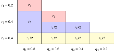
Figure 1: Toy demo illustrating how to obtain a non-uniform mini-batch sampling with batch size $b=2$ from $n=4$ coordinates.

6.3 Mini-batch adfSDCA algorithm

Here we describe a new adfSDCA algorithm that uses a mini-batch scheme. The algorithm is called mini-batch adfSDCA and is presented below as Algorithm 4.

Algorithm 4 Mini-Batch adfSDCA

1:  Input: Data: $\{x_{i},\phi_{i}\}_{i=1}^{n}$

2:  Initialization: Choose $\alpha^{(0)}\in\mathbb{R}^{n}$ and set batchsize $b$

3:  for $t=0,1,2,\dots$ do

4:     Calculate dual residue $\kappa^{(t)}_{i}=\phi^{\prime}_{i}(x_{i}^{T}w^{(t)})+\alpha^{(t)}_{i}$, for all $i\in[n]$

5:     Generate the adaptive probability distribution $p^{(t)}\sim\kappa^{(t)}$

6:     Choose mini-batch $S\subset[n]$ of size $b$ according to probabilities distribution $p^{(t)}$

7:     Set step-size $\theta^{(t)}\in(0,1)$ as in (75)

8:     for $i\in S$ do

9:        Update: $\alpha_{i}^{(t+1)}=\alpha_{i}^{(t)}-\theta^{(t)}(bp_{i}^{(t)})^{-1}\kappa^{(t)}_{i}$

10:     end for

11:     Update: $w^{(t+1)}=w^{(t)}-\sum_{i\in S}\theta^{(t)}(n\lambda bp_{i}^{(t)})^{-1}\kappa^{(t)}_{i}x_{i}$

12:  end for

Briefly, Algorithm 4 works as follows. At iteration $t$, adaptive probabilities are generated in the same way as for Algorithm 1. Then, instead of updating only one coordinate, a mini-batch $S$ of size $b\geq 1$ is chosen that is consistent with the adaptive probabilities. Next, the dual variables $\alpha_{i}^{(t)},i\in S$ are updated, and finally the primal variable $w$ is updated according to the primal-dual relation (4).

In the next section we will provide a convergence guarantee for Algorithm 4. As was discussed in Section 4, theoretical results are detailed under two different assumptions on the type of loss function: (i) all loss function are convex; and (ii) individual loss functions may be non-convex but the average over all loss functions is convex.

6.4 Expected Separable Overapproximation

Here we make use of the Expected Separable Overapproximation (ESO) theory introduced in Richtárik and Takáč (2012) and further extended, for example, in Qu and Richtárik (2016). The ESO definition is stated below.

Definition 4 (Expected Separable Overapproximation, Qu and Richtárik (2016)).

Let $\hat{S}$ be a sampling with marginal distribution $q=(q_{1},\cdots,q_{n})^{T}$. Then we say that the function $f$ admits a $v$-ESO with respect to the sampling $\hat{S}$ if $\forall x,h\in\mathbb{R}^{n}$, we have $v_{1},\dots,v_{n}>0$, such that the following inequality holds $\mathbf{E}[f(x+h_{[\hat{S}]})]\leq f(x)+\sum_{i=1}^{n}q_{i}(\nabla_{i}f(x)h_{i}+\tfrac{1}{2}v_{i}h_{i}^{2}).$

Remark 1.

Note that, here we do not assume that $\hat{S}$ is a uniform sampling, i.e., we do not assume that $q_{i}=q_{j}$ for all $i,j\in[n]$.

The ESO inequality is useful in this work because the parameter $v$ plays an important role when setting a suitable stepsize $\theta$ in our algorithm. Consequently, this also influences our complexity result, which depends on the sampling $\hat{S}$. For the proof of Theorem 4 (which will be stated in next subsection), the following is useful. Let $f(x)=\tfrac{1}{2}\|Ax\|^{2}$, where $A=(x_{1},\dots,x_{n})$. We say that $f(x)$ admits a $v$-ESO if the following inequality holds

$$\mathbf{E}[\|Ah_{\hat{S}}\|^{2}]\leq\sum_{i=1}^{n}v_{i}q_{i}h_{i}^{2}.$$ (33)

To derive the parameter $v$ we will make use of the following theorem.

Theorem 3 (Qu and Richtárik (2016)).

Let $f$ satisfy the following assumption $f(x+h)\leq f(x)+\langle\nabla f(x),h\rangle+\tfrac{1}{2}h^{T}A^{T}Ah^{T},$ where $A$ is some matrix. Then, for a given sampling $\hat{S}$, $f$ admits a $v$-ESO, where $v$ is defined by $v_{i}=\min\{\lambda^{\prime}(\mathbf{P}(\hat{S})),\lambda^{\prime}(A^{T}A)\}\sum_{j=1}^{m}A_{ji}^{2},i\in[n].$

Here $\mathbf{P}(\hat{S})$ is called a sampling matrix (see Richtárik and Takáč (2012)) where element $p_{ij}$ is defined to be $p_{ij}=\textstyle{\sum}_{\{i,j\}\in S,S\in\hat{S}}P(S).$ For any matrix $M$, $\lambda^{\prime}(M)$ denotes the maximal regularized eigenvalue of $M$, i.e., $\lambda^{\prime}(M)=\max_{\|h\|=1}\{h^{T}Mh:\textstyle{\sum}_{i=1}^{n}M_{ii}h_{i}^{2}\leq 1\}.$ We may now apply Theorem 3 because $f(x)=\tfrac{1}{2}\|Ax\|^{2}$ satisfies its assumption. Note that in our mini-batch setting, we have $P_{S\in\hat{S}}(|S|=b)=1$, so we obtain $\lambda^{\prime}(\mathbf{P}(\hat{S}))\leq b$ (Theorem 4.1 in Qu and Richtárik (2016)). In terms of $\lambda^{\prime}(A^{T}A)$, note that $\lambda^{\prime}(A^{T}A)=\lambda^{\prime}(\sum_{j=1}^{m}x_{j}x_{j}^{T})\leq\max_{j}\lambda^{\prime}(x_{j}x_{j}^{T})=\max_{j}|J_{j}|,$ where $|J_{j}|$ is number of non-zero elements of $x_{j}$ for each $j$. Then, a conservative choice from Theorem 3 that satisfies (33) is

$$v_{i}^{\prime}=\min\{b,\max_{j}|J_{j}|\}\|x_{i}\|^{2},\qquad i\in[n].$$ (34)

Now we are ready to give our complexity result for mini-batch adfSDCA (Algorithm 4). Note that we use the same notation as that established in Section 4 and we also define

$$Q^{\prime}\stackrel{{\scriptstyle\text{def}}}{{=}}\frac{1}{n}\sum_{i=1}^{n}v_{i}^{\prime}.$$ (35)

Theorem 4.

Let $\tilde{L}$, $\kappa_{i}^{(t)}$, $\gamma$ $D^{(t)}$, $v_{i}^{\prime}$, $C_{0}$ and $Q^{\prime}$ be as defined in (3), (5), (10), (11), (34), (19) and (35), respectively. Suppose that $\phi_{i}$ is $L$-smooth and convex for all $i\in[n]$. Then, at every iteration $t\geq 0$ of Algorithm 4, run with batchsize $b$ we have

$$\mathbf{E}[D^{(t+1)}|\alpha^{(t)}]\leq(1-\theta^{*})D^{(t)},$$ (36)

where $\theta^{*}=\tfrac{n\lambda^{2}b}{\sum_{i=1}^{n}(v_{i}^{\prime}\gamma+n\lambda^{2})}$. Moreover, it follows that whenever

$$T\geq\bigg{(}\frac{n}{b}+\frac{\tilde{L}Q^{\prime}}{b\lambda}\bigg{)}\log\bigg{(}\frac{(\lambda+\tilde{L})C_{0}}{\lambda\tilde{L}\epsilon}\bigg{)},$$ (37)

we have that $\mathbf{E}[P(w^{(T)}-P(w^{*}))]\leq\epsilon$.

It is also possible to derive a complexity result in the case when the average of the $n$ loss functions is convex. The theorem is stated now.

Theorem 5.

Let $L$, $\kappa_{i}^{(t)}$, $\bar{\gamma}$ $\bar{D}^{(t)}$, $v_{i}^{\prime}$, $\bar{C}_{0}$ and $Q^{\prime}$ be as defined in (3), (5), (24), (25), (34), (26) and (35) respectively. Suppose that every $\phi_{i},i\in[n]$ is $L_{i}$-smooth and that the average of the $n$ loss functions $\tfrac{1}{n}\sum_{i=1}^{n}\phi_{i}(w^{T}x_{i})$ is convex. Then, at every iteration $t\geq 0$ of Algorithm 4, run with batchsize $b$, we have

$$\mathbf{E}[\bar{D}^{(t+1)}|\alpha^{(t)}]\leq(1-\theta^{*})\bar{D}^{(t)},$$ (38)

where $\theta^{*}=\tfrac{n\lambda^{2}b}{\sum_{i=1}^{n}(v_{i}^{\prime}\bar{\gamma}+n\lambda^{2})}$. Moreover, it follows that whenever

$$T\geq\bigg{(}\frac{n}{b}+\frac{Q^{\prime}\frac{1}{n}\textstyle{\sum}_{i=1}^{n}L_{i}^{2}}{b\lambda}\bigg{)}\log\bigg{(}\frac{(\lambda+\tilde{L})\bar{C}_{0}}{\bar{\gamma}\epsilon}\bigg{)},$$ (39)

we have that $\mathbf{E}[P(w^{(T)}-P(w^{*})]\leq\epsilon$.

These theorems show that in worst case (by setting $b=1$), this mini-batch scheme shares the same complexity performance as the serial adfSDCA approach (recall Section 3). However, when the batch-size $b$ is larger, Algorithm 4 converges in fewer iterations. This behaviour will be confirmed computationally in the numerical results given in Section 7.

7 Numerical experiments

Here we present numerical experiments to demonstrate the practical performance of the adfSDCA algorithm. Throughout these experiments we used two loss functions, quadratic loss $\phi_{i}(w^{T}x_{i})=\tfrac{1}{2}(w^{T}x_{i}-y_{i})^{2}$ and logistic loss $\phi_{i}(w^{T}x_{i})=\log(1+\exp(-y_{i}w^{T}x_{i}))$. The experiments were run using datasets from the standard library of test problems (see Chang and Lin (2011) and http://www.csie.ntu.edu.tw/~cjlin/libsvm), as summarized in Table 1.

Dataset	#samples	#features	#classes	sparsity
w8a	$49,749$	$300$	$2$	$3.91\%$
mushrooms	$8,124$	$112$	$2$	$18.8\%$
ijcnn1	$49,990$	$22$	$2$	$59.1\%$
rcv1	$20,242$	$47,237$	$2$	$0.16\%$
news20	$19,996$	$1,355,191$	$2$	$0.034\%$

Table 1: The datasets used in the numerical experiments Chang and Lin (2011).

7.1 Comparison for a variety of dfSDCA approaches

In this section we compare the adfSDCA algorithm (Algorithm 1) with both dfSCDA, which is a uniform variant of adfSDCA described in Shalev-Shwartz (2015), and also with Prox-SDCA from Shalev-Shwartz and Zhang (2014). We also report results using Algorithm 2, which is a heuristic version of adfSDCA, used with several different shrinking parameters.

Figures 2 and 3 compare the evolution of the duality gap for the standard and heuristic variant of our adfSDCA algorithm with the two state-of-the-art algorithms dfSDCA and Prox-SDCA. For these problems both our algorithm variants out-perform the dfSDCA and Prox-SDCA algorithms. Note that this is consistent with our convergence analysis (recall Section 4). Now consider the adfSDCA+ algorithm, which was tested using the parameter values $s=1,10,20$. It is clear that adfSDCA+ with $s=1$ shows the worst performance, which is reasonable because in this case the algorithm only updates the sampling probabilities after each epoch; it is still better than dfSDCA since it utilizes the sub-optimality at the beginning of each epoch. On the other hand, there does not appear to be an obvious difference between adfSDCA+ used with $s=10$ or $s=20$ with both variants performing similarly. We see that adfSDCA performs the best overall in terms of the number of passes through the data. However, in practice, even though adfSDCA+ may need more passes through the data to obtain the same sub-optimality as adfSDCA, it requires less computational effort than adfSDCA.

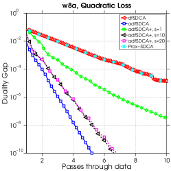
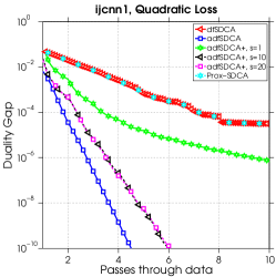
Figure 2: A comparison of the number of epochs versus the duality gap for the various algorithms.

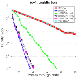
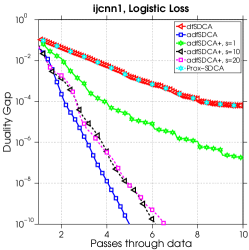
Figure 3: A comparison of the number of epochs versus the duality gap for the various algorithms.

Figure 4 shows the estimated density function of the dual residue $|\kappa^{(t)}|$ after $1,2,3,4$ and $5$ epochs for both uniform dfSDCA and our adaptive adfSDCA. One observes that the adaptive scheme is pushing the large residuals towards zero much faster than uniform dfSDCA. For example, notice that after $2$ epochs, almost all residuals are below $0.03$ for adfSDCA, whereas for uniform dfSDCA there are still many residuals larger than $0.06$. This is evidence that, by using adaptive probabilities we are able to update the coordinate with a high dual residue more often and therefore reduce the sub-optimality much more efficiently.

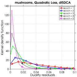
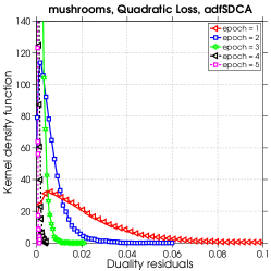
Figure 4: Comparing absolute value of dual residuals at each epoch between dfSDCA and adfSDCA.

7.2 Mini-batch SDCA

Here we investigate the behaviour of the mini-batch adfSDCA algorithm (Algorithm 4). In particular, we compare the practical performance of mini-batch adfSDCA using different mini-batch sizes $b$ varying from $1$ to $32$. Note that if $b=1$, then Algorithm 4 is equivalent to the adfSDCA algorithm (Algorithm 1). Figures 5 and 6 show that, with respect to the different batch sizes, the mini-batch algorithm with each batch size needs roughly the same number of passes through the data to achieve the same sub-optimality. However, when considering the computational time, the larger the batch size is, the faster the convergence will be. Recall that the results in Section 6 show that the number of iterations needed by Algorithm 4 used with a batch size of $b$ is roughly $1/b$ times the number of iterations needed by adfSDCA. Here we compute the adaptive probabilities every $b$ samples, which leads to roughly the same number of passes through the data to achieve the same sub-optimality.

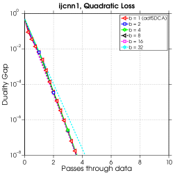
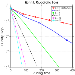
Figure 5: Comparing the number of iterations of various batch size on a quadratic loss.

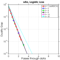
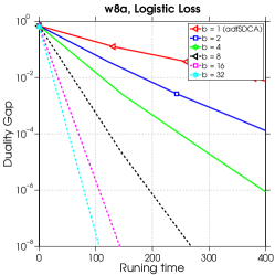
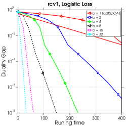
Figure 6: Comparing number of iterations among various batch size on logistic loss.

Appendix A Appendix

A.1 Preliminaries and Technical Results

Recall that $w^{*}$ denotes an optimum of (P) and define $\alpha_{i}^{*}=-\phi^{\prime}_{i}(x_{i}^{T}w^{*})$. To simplify the proofs we introduce the following variables

$$A^{(t)}=\tfrac{1}{n}\|\alpha^{(t)}-\alpha^{*}\|^{2}~{}\mbox{and}~{}B^{(t)}=\|w^{(t)}-w^{*}\|^{2}.$$ (40)

At the optimum $w^{*}$, it holds that $0=\nabla P(w^{*})=\frac{1}{n}\sum_{i=1}^{n}\phi^{\prime}_{i}(x_{i}^{T}w^{*})x_{i}+\lambda w^{*}$, so $w^{*}=\frac{1}{\lambda n}\sum_{i=1}^{n}\alpha_{i}^{*}x_{i}$. Define $u_{i}^{(t)}\stackrel{{\scriptstyle\text{def}}}{{=}}-\phi^{\prime}_{i}(x_{i}^{T}w^{(t)})$, and therefore we have $\kappa_{i}^{(t)}=\alpha_{i}^{(t)}-u_{i}^{(t)}$ and $u_{i}^{*}=\alpha_{i}^{*}$.

The following two lemmas will be useful when proving our main results.

Lemma 4.

Let $A^{(t)}$ and $B^{(t)}$ be defined in (40), and let $v_{i}=\|x_{i}\|^{2}$ for all $i\in[n]$. Then, conditioning on $\alpha^{(t)}$, the following hold for given $\theta$:

$$\mathbf{E}[A^{(t+1)}|\alpha^{(t)}]-A^{(t)} =-\theta A^{(t)}+\frac{\theta}{n}\sum_{i=1}^{n}\Big{(}(u_{i}^{(t)}-\alpha_{i}^{*})^{2}-\big{(}1-\tfrac{\theta}{p_{i}}\big{)}(\kappa_{i}^{(t)})^{2}\Big{)},$$ (41)

$$\mathbf{E}[B^{(t+1)}|\alpha^{(t)}]-B^{(t)} =-\tfrac{2\theta}{\lambda}(w^{(t)}-w^{*})^{T}\nabla P(w^{(t)})+\sum_{i=1}^{n}\frac{\theta^{2}v_{i}}{n^{2}\lambda^{2}p_{i}}\big{(}\kappa^{(t)}_{i}\big{)}^{2}.$$ (42)

Proof.

Note that at iteration $t$, only coordinate $i$ (of $\alpha$) is updated, so

$$A^{(t+1)}=\tfrac{1}{n}\|\alpha^{(t+1)}-\alpha^{*}\|^{2}\equiv\frac{1}{n}\sum_{j\neq i}(\alpha_{j}^{(t)}-\alpha_{j}^{*})^{2}+\frac{1}{n}(\alpha_{i}^{(t+1)}-\alpha_{i}^{*})^{2}.$$ (43)

Thus,

$$A^{(t+1)}-A^{(t)}\overset{\eqref{eq:intA}}{=} \tfrac{1}{n}(\alpha_{i}^{(t+1)}-\alpha_{i}^{*})^{2}-\tfrac{1}{n}(\alpha_{i}^{(t)}-\alpha_{i}^{*})^{2}$$

$$= \tfrac{1}{n}\Big{(}\alpha_{i}^{(t)}-\tfrac{\theta}{p_{i}}\kappa_{i}^{(t)}-\alpha_{i}^{*}\Big{)}^{2}-\tfrac{1}{n}(\alpha_{i}^{(t)}-\alpha_{i}^{*})^{2}$$

$$= \tfrac{1}{n}\left(\big{(}1-\tfrac{\theta}{p_{i}}\big{)}(\alpha_{i}^{(t)}-\alpha_{i}^{*})-\tfrac{\theta}{p_{i}}(\kappa_{i}^{(t)}-\alpha_{i}^{*})\right)^{2}-\tfrac{1}{n}(\alpha_{i}^{(t)}-\alpha_{i}^{*})^{2}$$

$$= \tfrac{1}{n}\left(1-\tfrac{\theta}{p_{i}}\right)(\alpha_{i}^{(t)}-\alpha_{i}^{*})^{2}+\tfrac{\theta}{np_{i}}(u_{i}^{(t)}-\alpha_{i}^{*})^{2}-\left(1-\tfrac{\theta}{p_{i}}\right)\tfrac{\theta}{np_{i}}(\kappa_{i}^{(t)})^{2}-\tfrac{1}{n}(\alpha_{i}^{(t)}-\alpha_{i}^{*})^{2}$$

$$= -\tfrac{\theta}{np_{i}}(\alpha_{i}^{(t)}-\alpha_{i}^{*})^{2}+\tfrac{\theta}{np_{i}}\left((u_{i}^{(t)}-\alpha_{i}^{*})^{2}-\left(1-\tfrac{\theta}{p_{i}}\right)(\kappa_{i}^{(t)})^{2}\right).$$ (44)

Taking expectation over $i\in[n]$, conditioned on $\alpha^{(t)}$, gives the first result.

To obtain the second result consider

$$B^{(t+1)}-B^{(t)} \overset{\eqref{eq:AB}}{=} \|w^{(t+1)}-w^{*}\|^{2}-\|w^{(t)}-w^{*}\|^{2}$$

$$\overset{\eqref{wupdate}}{=} \|w^{(t)}-\tfrac{\theta}{n\lambda p_{i}}\kappa_{i}^{(t)}x_{i}-w^{*}\|^{2}-\|w^{(t)}-w^{*}\|^{2}$$

$$= -\tfrac{2\theta}{n\lambda p_{i}}\kappa_{i}^{(t)}x_{i}^{T}(w^{(t)}-w^{*})+\tfrac{\theta^{2}v_{i}}{n^{2}\lambda^{2}p_{i}^{2}}(\kappa_{i}^{(t)})^{2}.$$

Recall that $\mathbf{E}[\frac{1}{np_{i}}\kappa_{i}^{(t)}x_{i}]=\nabla P(w^{(t)})$ by (9). Thus, taking expectation over $i\in[n]$, conditioned on $w^{(t)}$, gives (42).∎∎

The following Lemma and proof are similar to (Csiba and Richtárik, 2015, Lemma 4) and (Shalev-Shwartz and Zhang, 2013, Lemma 1).

Lemma 5.

Assume that each $\phi_{i}$ is $\tilde{L}_{i}$-smooth and convex. Then, for every $w$

$$\frac{1}{\tilde{L}}\Big{(}\frac{1}{n}\sum_{i=1}^{n}\|\phi^{\prime}_{i}(x_{i}^{T}w)-\phi^{\prime}_{i}(x_{i}^{T}w^{*})\|^{2}\Big{)} \leq\frac{1}{n}\sum_{i=1}^{n}\frac{1}{\tilde{L}_{i}}\|\phi^{\prime}_{i}(w^{T}x_{i})-\phi^{\prime}_{i}(x_{i}^{T}w^{*})\|^{2}$$

$$\leq 2\left(P(w)-P(w^{*})-\tfrac{\lambda}{2}\|w-w^{*}\|^{2}\right).$$ (45)

Proof.

Let $z,z^{*}\in\mathbb{R}$. Define

$$g_{i}(z)\stackrel{{\scriptstyle\text{def}}}{{=}}\phi_{i}(z)-\phi_{i}(z^{*})-\phi^{\prime}_{i}(z^{*})(z-z^{*}).$$ (46)

Because $\phi_{i}$ is $\tilde{L}_{i}$-smooth, so too is $g_{i}$, which implies that for all $z,\hat{z}\in\mathbb{R}$,

$$g_{i}(z)\leq g_{i}(\hat{z})+g^{\prime}_{i}(\hat{z})(z-\hat{z})+\tfrac{\tilde{L}_{i}}{2}(z-\hat{z})^{2}.$$ (47)

By convexity of $\phi_{i}$, $g_{i}$ is nonnegative, i.e., $g_{i}(z)\geq 0$ for all $z$. Hence, by non-negativity and smoothness $g_{i}$ is self-bounded (see Section 12.1.3 in Shalev-Shwartz and Ben-David (2014) or set $z=\hat{z}-\frac{1}{\tilde{L}_{i}}g^{\prime}_{i}(\hat{z})$ in (47) and rearrange):

$$\|g^{\prime}_{i}(z)\|^{2}\leq 2\tilde{L}_{i}g_{i}(z),\qquad\forall z.$$ (48)

Differentiating (46) w.r.t. $z$ and combining the result with (48), used with $z=x_{i}^{T}w$ and $z^{*}=x_{i}^{T}w^{*}$, gives

$$\|\phi^{\prime}_{i}(x_{i}^{T}w)-\phi^{\prime}_{i}(x_{i}^{T}w^{*})\|^{2}=\|g^{\prime}_{i}(x_{i}^{T}w)\|^{2}\leq 2\tilde{L}_{i}g_{i}(x_{i}^{T}w).$$ (49)

Multiplying (49) through by $1/(n\tilde{L}_{i})$ and summing over $i\in[n]$ shows that

$$\frac{1}{n}\sum_{i=1}^{n}\frac{1}{\tilde{L}_{i}}\|\phi^{\prime}_{i}(x_{i}^{T}w)-\phi^{\prime}_{i}(x_{i}^{T}w^{*})\|^{2}\leq\frac{2}{n}\sum_{i=1}^{n}g_{i}(x_{i}^{T}w)$$

$$=~{} \frac{2}{n}\sum_{i=1}^{n}\phi_{i}(x_{i}^{T}w)-\phi_{i}(x_{i}^{T}w^{*})-\phi^{\prime}_{i}(x_{i}^{T}w^{*})(x_{i}^{T}w-x_{i}^{T}w^{*})$$

$$=~{} 2\left(P(w)-\tfrac{\lambda}{2}\|w\|^{2}-P(w^{*})+\tfrac{\lambda}{2}\|w^{*}\|^{2}-\lambda(w^{*})^{T}(w-w^{*})\right)$$

$$=~{} 2\left(P(w)-P(w^{*})-\tfrac{\lambda}{2}\|w-w^{*}\|^{2}\right),$$

where we have used the fact that $\mathbf{E}[\nabla P(w^{*})]=\mathbf{E}[\phi^{\prime}(x_{i}^{T}w^{*})x_{i}+\lambda w^{*}]=0.$ The first inequality follows because $\tilde{L}=\max_{i}\tilde{L}_{i}$.∎∎

A.2 Proof of Lemmas 1 and 3

Proof of Lemma 1.

In this case it is assumed that every loss function is convex and we set $\gamma=\lambda\tilde{L}$ (10). For convenience, define the following quantities:

$$\mathbf{C_{1}}\stackrel{{\scriptstyle\text{def}}}{{=}}\frac{\theta}{n}\sum_{i=1}^{n}(u_{i}^{(t)}-\alpha_{i}^{*})^{2}-\tfrac{2\gamma\theta}{\lambda}\nabla P(w^{(t)})^{T}(w^{(t)}-w^{*})$$ (50)

$$\mathbf{C_{2}}\stackrel{{\scriptstyle\text{def}}}{{=}}\sum_{i=1}^{n}\Big{(}-\tfrac{\theta}{n}(1-\tfrac{\theta}{p_{i}})+\tfrac{\theta^{2}v_{i}\gamma}{n^{2}\lambda^{2}p_{i}}\Big{)}(\kappa_{i}^{(t)})^{2}$$ (51)

Recall that $A^{(t)}$, $B^{(t)}$ and $D^{(t)}$ are defined in (40) and (11), respectively, and $\gamma$ is defined in (10). Then,

$$\mathbf{E}[D^{(t+1)}|\alpha^{(t)}]-D^{(t)}=~{}~{} \mathbf{E}[A^{(t+1)}-A^{(t)}|\alpha^{(t)}]+\gamma\mathbf{E}[B^{(t+1)}-B^{(t)}|\alpha^{(t)}]$$

$$\overset{\mathclap{\eqref{eq: E[A]},\eqref{eq: E[B]}}}{=}~{}~{} -\theta A^{(t)}+\tfrac{\theta}{n}\sum_{i=1}^{n}\left((u_{i}^{(t)}-\alpha_{i}^{*})^{2}-\Big{(}1-\tfrac{\theta}{p_{i}}\Big{)}(\kappa_{i}^{(t)})^{2}\right)$$

$$+\gamma\bigg{(}-\tfrac{2\theta}{\lambda}\nabla P(w^{(t)})^{T}(w^{(t)}-w^{*})+\sum_{i=1}^{n}\frac{\theta^{2}v_{i}}{n^{2}\lambda^{2}p_{i}}(\kappa^{(t)}_{i})^{2}\bigg{)}$$

$$\overset{\mathclap{\eqref{eq:C1},\eqref{eq:C2}}}{\leq}~{}~{} -\theta A^{(t)}+\mathbf{C_{1}}+\mathbf{C_{2}}.$$ (52)

Now,

$$\mathbf{C_{1}} \overset{\eqref{eq:C1}}{=} \frac{\theta}{n}\sum_{i=1}^{n}(u_{i}^{(t)}-\alpha_{i}^{*})^{2}-\tfrac{2\gamma\theta}{\lambda}\nabla P(w^{(t)})^{T}(w^{(t)}-w^{*})$$ (53)

$$\overset{\mathclap{(\ref{eq: strong ineq})}}{\leq} 2\theta\tilde{L}\left(P(w^{(t)})-P(w^{*})-\tfrac{\lambda}{2}\|w^{(t)}-w^{*}\|^{2}\right)-\tfrac{2\gamma\theta}{\lambda}\nabla P(w^{(t)})^{T}(w^{(t)}-w^{*})$$

$$\overset{\mathclap{\gamma=\lambda\tilde{L}}}{=} -\gamma\theta\|w^{(t)}-w^{*}\|^{2}+2\theta\tilde{L}\left(P(w^{(t)})-P(w^{*})-\nabla P(w^{(t)})^{T}(w^{(t)}-w^{*})\right)$$

$$\leq -\gamma\theta\|w^{(t)}-w^{*}\|^{2},$$

where the last inequality follows from convexity of $P(w)$, i.e., $P(w^{(t)})-P(w^{*})\leq\nabla P(w^{(t)})^{T}(w^{(t)}-w^{*})$. Combining (A.2) and (53) gives

$$\mathbf{E}[D^{(t+1)}|\alpha^{(t)}]-D^{(t)}\leq-\theta A^{(t)}-\gamma\theta\|w^{(t)}-w^{*}\|^{2}+\mathbf{C_{2}}=-\theta D^{(t)}+\mathbf{C_{2}}.$$

Rearranging gives the result.∎∎

Proof of Lemma 3.

For this result we assume that the average of the loss functions $\frac{1}{n}\sum\phi_{i}(\cdot)$ is convex. Note that one can define parameters $\mathbf{\bar{C}_{1}}$ and $\mathbf{\bar{C}_{2}}$ that are analogous to $\mathbf{C_{1}}$ and $\mathbf{C_{2}}$ in (50) and (51) but with $\gamma$ replaced by $\bar{\gamma}$. Then, the same arguments as those used in (A.2) can be used to show that

$$\mathbf{E}[\bar{D}^{(t+1)}|\alpha^{(t)}]-\bar{D}^{(t)}\leq-\theta A^{(t)}+\mathbf{\bar{C}_{1}}+\mathbf{\bar{C}_{2}}.$$ (54)

Now, note that by Lipschitz continuity of $\phi^{\prime}(\cdot)$ one has

$$(u_{i}^{(t)}-\alpha_{i}^{*})^{2}=\left(\phi^{\prime}_{i}(x_{i}^{T}w)-\phi^{\prime}_{i}(x_{i}^{T}w^{(t)})\right)^{2}\leq L_{i}^{2}\|w^{*}-w^{(t)}\|^{2}.$$ (55)

Further, since the average of the losses is convex, $P(w)$ is strongly convex, so

$$P(w^{*})-P(w^{(t)})\geq\nabla P(w^{(t)})^{T}(w^{*}-w^{(t)})+\tfrac{\lambda}{2}\|w^{*}-w^{(t)}\|^{2}$$ (56)

and since $w^{*}$ is the minimizer

$$P(w^{t})-P(w^{*})\geq\tfrac{\lambda}{2}\|w^{(t)}-w^{*}\|^{2}.$$ (57)

Now, adding (56) and (57) gives

$$\nabla P(w^{(t)})^{T}(w^{(t)}-w^{*})\geq\lambda\|w^{(t)}-w^{*}\|^{2}.$$ (58)

Therefore,

$$\mathbf{\bar{C}_{1}}=~{}~{} \frac{\theta}{n}\sum_{i=1}^{n}(u_{i}^{(t)}-\alpha_{i}^{*})^{2}-\frac{2\bar{\gamma}\theta}{\lambda}\nabla P(w^{(t)})^{T}(w^{(t)}-w^{*})$$

$$\overset{\eqref{eq:Lipschitz},\eqref{eq:gradPnormw}}{\leq}~{}~{} \frac{\theta}{n}\sum_{i=1}^{n}L_{i}^{2}\|w^{(t)}-w^{*}\|^{2}-2\bar{\gamma}\theta\|w^{(t)}-w^{*}\|^{2}$$

$$\overset{\eqref{eq:bargamma}}{\leq}~{}~{} -\bar{\gamma}\theta\|w^{(t)}-w^{*}\|^{2}.$$ (59)

Thus, from (54) and (A.2) we have that $\mathbf{E}[D^{(t+1)}|\alpha^{(t)}]-D^{(t)}\leq-\theta D^{(t)}+{\mathbf{\bar{C}_{2}}}$, which is the desired result.∎∎

A.3 Proof of Lemma 2

Proof.

This is easy to verify by derive KKT conditions of optimization problem (16), which is

$$\begin{cases}-(n\lambda^{2}\sum_{i\in I_{\kappa}}\kappa_{i}^{2})(\sum_{i\in I_{\kappa}}(n\lambda^{2}+v_{i}\gamma)p_{i}^{-1}\kappa_{i}^{2})^{-2}(-(n\lambda^{2}+v_{i}\gamma)p_{i}^{-2}\kappa_{i}^{2})+\mu&=0\\ \sum_{i\in I_{k}}p_{i}&=1\\ \end{cases}$$

where $\mu$ is the Lagrange multiplier.

Therefore, we have

$$\frac{p_{i}}{p_{j}}=\frac{\sqrt{n\lambda^{2}+v_{i}\gamma}|\kappa_{i}|}{\sqrt{n\lambda^{2}+v_{j}\gamma}|\kappa_{j}|},\mbox{ for all }i,j\in I_{\kappa}.$$ (60)

Considering $\sum_{i\in I_{\kappa}}p_{i}=1$, we show that the optimal probabilities (17). (18) can be further derived by combine (17) and (16). ∎

A.4 Proof of Theorems 1 and 2

Proof of Theorem 1.

Note that substituting $p^{*}$ (where $p^{*}$ is defined in Lemma 2) into $\Theta(\kappa,p^{*})$ in (15) and using the Cauchy-Schwartz inequality, gives

$$\Theta(\kappa,p^{*})=\frac{n\lambda^{2}\sum_{i\in I_{\kappa}}\kappa_{i}^{2}}{(\sum_{i\in I_{\kappa}}\sqrt{v_{i}\gamma+n\lambda^{2}}|\kappa_{i}|)^{2}}=\frac{n\lambda^{2}\sum_{i=1}^{n}\kappa_{i}^{2}}{(\sum_{i=1}^{n}\sqrt{v_{i}\gamma+n\lambda^{2}}|\kappa_{i}|)^{2}}\geq\frac{n\lambda^{2}}{\sum_{i=1}^{n}(v_{i}\gamma+n\lambda^{2})}\overset{\eqref{eq:thetastar}}{=}\theta^{*}.$$ (61)

The above confirms that $\theta^{*}$ in (15) is a (constant) global lower bound of $\Theta(\kappa,p^{*})$ at every iteration. Thus, using the arguments following Lemma 1, setting $p^{(t)}=p^{*}$ (as computed in Lemma 2) at each iteration gives

$$\mathbf{E}\left[D^{(t+1)}|\alpha^{(t)}\right]\leq(1-\theta^{*})D^{(t)}.$$ (62)

That is, (14) used with $\theta\equiv\theta^{*}$ holds. Because (62) holds at every iteration of Algorithm 1, one can show that

$$\mathbf{E}\left[D^{(t)}\right]\leq(1-\theta^{*})^{t}C_{0}\leq e^{-\theta^{*}t}C_{0},$$ (63)

where $C_{0}$ is defined in (19). Now, note that $P(w)$ is $(L+\lambda)$-smooth, i.e., $P(w)-P(w^{*})\leq\tfrac{\lambda+L}{2}\|w-w^{*}\|^{2}$, so

$$D^{(t)}=\tfrac{1}{n}\|\alpha^{(t)}-\alpha^{*}\|^{2}+\gamma\|w^{(t)}-w^{*}\|^{2}\geq\gamma\|w^{(t)}-w^{*}\|^{2}\geq\tfrac{2\gamma}{\lambda+L}(P(w^{(t)})-P(w^{*})).$$

This means that we must find $T$ for which

$$\mathbf{E}[P(w^{(T)})-P(w^{*})]\leq\tfrac{\lambda+L}{2\gamma}e^{-\theta^{*}T}C_{0}\leq\epsilon.$$ (64)

Subsequently, the expression for $T$ in (23) is obtained by multiplying through by $e^{\theta^{*}T}/\epsilon$, taking natural logs, rearranging and noting that

$$\frac{1}{\theta^{*}}=\frac{\sum_{i=1}^{n}(v_{i}\gamma+n\lambda^{2})}{n\lambda^{2}}=n+\frac{\gamma}{n\lambda^{2}}\sum_{i=1}^{n}v_{i}\overset{\eqref{eq:gamma}}{=}n+\frac{\tilde{L}}{n\lambda}\sum_{i=1}^{n}v_{i}\overset{\eqref{eq:MQ}}{=}n+\frac{\tilde{L}Q}{\lambda}.$$

∎

Proof of Theorem 2.

Here we assume that the average loss $\frac{1}{n}\sum_{i=1}^{n}\phi_{i}(\cdot)$ is convex, but that individual loss functions $\phi_{i}(\cdot)$ may not be. The proof of this result is almost identical to the proof of Theorem 1, but with the parameters defined in Section 4.2. Similarly to (64) we must find $T$ for which

$$\mathbf{E}[P(w^{(T)})-P(w^{*})]\leq\tfrac{\lambda+L}{2\bar{\gamma}}e^{-\theta^{*}T}\bar{C}_{0}\leq\epsilon,$$ (65)

where $\bar{\gamma}=\frac{1}{n}\sum_{i=1}^{n}L_{i}^{2}$ is defined in (24) and $\bar{C}_{0}$ is defined in (26). The expression $T$ in (30) is obtained by multiplying through by $e^{\theta^{*}T}/\epsilon$, taking natural logs, rearranging and noting that

$$\frac{1}{\theta^{*}}=\frac{\sum_{i=1}^{n}(v_{i}\bar{\gamma}+n\lambda^{2})}{n\lambda^{2}}=n+\frac{\bar{\gamma}}{\lambda^{2}}\Big{(}\frac{1}{n}\sum_{i=1}^{n}v_{i}\Big{)}\overset{\eqref{eq:MQ}}{=}n+\frac{\bar{\gamma}Q}{\lambda^{2}}.$$

∎∎

A.5 Proof of Corollary 1

Proof.

Recall that $w^{*}$ denotes the minimizer of (P) and $\alpha_{i}^{*}=-\phi^{\prime}(x_{i}^{T}w^{*})$. Let Assumption 2 hold. Then

$$\Big{\|}\frac{1}{np_{i}}\kappa_{i}^{(t)}x_{i}\Big{\|}^{2} \overset{\eqref{eq:viQ}}{=} \frac{1}{n^{2}p_{i}^{2}}(\kappa_{i}^{(t)})^{2}v_{i}$$ (66)

$$\overset{\mathclap{\eqref{eq: optimal probabilities}}}{=} \frac{1}{n^{2}}\left(\frac{\sum_{j\in I_{\kappa}}\sqrt{n\lambda^{2}+v_{j}\gamma}|\kappa_{j}^{(t)}|}{\sqrt{n\lambda^{2}+v_{i}\gamma}|\kappa_{i}^{(t)}|}\right)^{2}(\kappa_{i}^{(t)})^{2}v_{i}$$

$$\overset{\rm(CS)}{\leq} \frac{1}{n^{2}}\frac{\sum_{j=1}^{n}(n\lambda^{2}+v_{j}\gamma)\sum_{j=1}^{n}(\kappa_{j}^{(t)})^{2}}{(n\lambda^{2}+v_{i}\gamma)(\kappa_{i}^{(t)})^{2}}(\kappa_{i}^{(t)})^{2}v_{i}$$

$$= \frac{\sum_{j=1}^{n}(n\lambda^{2}+v_{j}\gamma)}{n^{2}(n\lambda^{2}+v_{i}\gamma)}\|\kappa^{(t)}\|^{2}v_{i}$$

$$\overset{\eqref{eq:MQ}}{=} \frac{n^{2}\lambda^{2}+\gamma nQ}{n^{2}(n\lambda^{2}+v_{i}\gamma)}\|\kappa^{(t)}\|^{2}v_{i}.$$

Taking the (conditional) expectation of (66) gives

$$\mathbf{E}\left[\Big{\|}\frac{1}{np_{i}}\kappa_{i}^{(t)}x_{i}\Big{\|}^{2}\,\Big{|}\alpha^{(t-1)}\right] = \sum_{i=1}^{n}p_{i}\left(\frac{n^{2}\lambda^{2}+\gamma nQ}{n^{2}(n\lambda^{2}+v_{i}\gamma)}\|\kappa^{(t)}\|^{2}v_{i}\right)$$ (67)

$$\leq \sum_{i=1}^{n}\left(\frac{n^{2}\lambda^{2}+\gamma nQ}{n^{2}(n\lambda^{2}+v_{i}\gamma)}\|\kappa^{(t)}\|^{2}v_{i}\right)$$

$$\leq \sum_{i=1}^{n}\left(\frac{n^{2}\lambda^{2}+\gamma nQ}{n^{3}\lambda^{2}}\|\kappa^{(t)}\|^{2}v_{i}\right)$$

$$= \left(\frac{n^{2}\lambda^{2}+\gamma nQ}{n^{2}\lambda^{2}}\|\kappa^{(t)}\|^{2}\right)\left(\frac{1}{n}\sum_{i=1}^{n}v_{i}\right)$$

$$\overset{\eqref{eq:MQ}}{=} Q\left(1+\frac{\gamma Q}{n\lambda^{2}}\right)\|\kappa^{(t)}\|^{2}.$$

Finally

$$\|\kappa^{(t)}\|^{2}=\mathbf{E}\left[\|\kappa^{(t)}\|^{2}|\alpha^{(t-1)}\right]=~{}~{} \mathbf{E}\Big{[}\sum_{i=1}^{n}\Big{(}\alpha^{(t)}_{i}+\phi^{\prime}_{i}(x_{i}^{T}w^{(t)})\Big{)}^{2}|\alpha^{(t-1)}\Big{]}$$

$$=~{}~{} \mathbf{E}\Big{[}\sum_{i=1}^{n}\Big{(}\alpha^{(t)}_{i}-\alpha^{*}-\phi^{\prime}_{i}(x_{i}^{T}w^{*})+\phi^{\prime}_{i}(x_{i}^{T}w^{(t)})\Big{)}^{2}|\alpha^{(t-1)}\Big{]}$$

$$\leq~{}~{} 2\mathbf{E}[\|\alpha^{(t)}-\alpha^{*}\|^{2}|\alpha^{(t-1)}]+2L\mathbf{E}[\|w^{(t)}-w^{*}\|^{2}|\alpha^{(t-1)}].$$

Combining the last step with (67) gives the result. ∎∎

The proof of Corollary 2 is essentially identical, but with the notation established in Section 4.2, so we omit it for brevity.

A.6 Proof of Theorems 4 and 5

Recall that $A^{(t)}$ and $B^{(t)}$ are defined in (40). To prove Theorem 4 we need the following two conditions to hold,

$$\mathbf{E}_{\hat{S}}\left[A^{(t+1)}-A^{(t)}|\alpha^{(t)}\right]= -\theta A^{(t)}+\frac{\theta}{n}\sum_{i=1}^{n}\left((u_{i}^{(t)}-\alpha_{i}^{*})^{2}-\left(1-\tfrac{\theta}{bp_{i}}\right)(\kappa^{(t)}_{i})^{2}\right),$$ (68)

$$\mathbf{E}_{\hat{S}}\left[B^{(t+1)}-B^{(t)}|\alpha^{(t)}\right]\leq -\frac{2\theta}{\lambda}\nabla P(w^{(t)})^{T}(w^{(t)}-w^{*})+\sum_{i=1}^{n}\frac{\theta^{2}v_{i}(\kappa^{(t)}_{i})^{2}}{n^{2}\lambda^{2}bp_{i}}.$$ (69)

Note that $\mathbf{E}_{\hat{S}}\left[A^{(t+1)}-A^{(t)}|\alpha^{(t)}\right]=\sum_{i=1}^{n}bp_{i}(A^{(t+1)}-A^{(t)})$, and so (68) is obtained by using arguments similar to those used in the proof of (41). To show (69), first we have

$$B^{(t+1)}-B^{(t)} =\|w^{(t+1)}-w^{*}\|^{2}-\|w^{(t)}-w^{*}\|^{2}$$

$$=\|w^{(t)}-\sum_{i\in S}\frac{\theta}{n\lambda bp_{i}}\kappa_{i}^{(t)}x_{i}^{T}-w^{*}\|^{2}-\|w^{(t)}-w^{*}\|^{2}$$

$$=-\frac{2\theta}{n\lambda}\sum_{i\in S}\frac{\kappa^{(t)}_{i}}{bp_{i}}x_{i}^{T}(w^{(t)}-w^{*})+\frac{\theta^{2}}{n^{2}\lambda^{2}}\|\sum_{i\in S}\frac{\kappa_{i}^{(t)}}{bp_{i}}x_{i}\|^{2}.$$ (70)

Therefore, we have

$$\mathbf{E}_{\hat{S}}\left[B^{(t+1)}-B^{(t)}|\alpha^{(t)}\right] =\mathbf{E}_{\hat{S}}\bigg{[}-\frac{2\theta}{n\lambda}\sum_{i\in S}\frac{\kappa^{(t)}_{i}}{bp_{i}}x_{i}^{T}(w^{(t)}-w^{*})+\frac{\theta^{2}}{n^{2}\lambda^{2}}\|\sum_{i\in S}\frac{\kappa_{i}^{(t)}}{bp_{i}}x_{i}\|^{2}|\alpha^{(t)}\bigg{]}$$

$$=-\frac{2\theta}{n\lambda}\sum_{i=1}^{n}\kappa_{i}^{(t)}x_{i}^{T}(w^{(t)}-w^{*})+\frac{\theta^{2}}{n^{2}\lambda^{2}}\mathbf{E}_{\hat{S}}\|\sum_{i\in S}\frac{\kappa_{i}^{(t)}}{bp_{i}}x_{i}\|^{2}.$$ (71)

Note that from Section 6.4 we have

$$\mathbf{E}_{\hat{S}}\|\sum_{i\in S}\frac{\kappa_{i}^{(t)}}{bp_{i}}x_{i}\|^{2}\leq\sum_{i=1}^{n}bp_{i}v_{i}^{\prime}\bigg{(}\frac{\kappa_{i}^{(i)}}{bp_{i}}\bigg{)}^{2}=\sum_{i=1}^{n}\frac{v_{i}^{\prime}(\kappa_{i}^{(t)})^{2}}{bp_{i}},$$ (72)

where $v_{i}^{\prime}$ is defined in (34). We can then derive (69) by using (72) and $\nabla P(w^{(t)})=\frac{1}{n}\sum_{i=1}^{n}\kappa_{i}^{(t)}x_{i}$.

Proof of Theorem 4.

Define

$$\mathbf{C}(\theta,p^{(t)},\kappa^{(t)})\stackrel{{\scriptstyle\text{def}}}{{=}}\sum_{i=1}^{n}\left(-\frac{\theta}{n}\Big{(}1-\frac{\theta}{bp_{i}}\Big{)}+\frac{\theta^{2}v_{i}^{\prime}\gamma}{n^{2}\lambda^{2}bp_{i}}\right)(\kappa_{i}^{(t)})^{2}.$$ (73)

Then

$$\mathbf{E}_{\hat{S}}[D^{(t+1)}-D^{(t)}|\alpha^{(t)}] = \mathbf{E}_{\hat{S}}[A^{(t+1)}-A^{(t)}|\alpha^{(t)}]+\gamma\mathbf{E}_{\hat{S}}[B^{(t+1)}-B^{(t)}|\alpha^{(t)}]$$ (74)

$$\overset{\mathclap{\eqref{eq: ES[A]},\eqref{eq: ES[B]}}}{\leq}~{}~{} -\theta A^{(t)}+\frac{\theta}{n}\sum_{i=1}^{n}\left(\Big{(}u_{i}^{(t)}-\alpha_{i}^{*})^{2}-(1-\frac{\theta}{bp_{i}}\Big{)}(\kappa^{(t)}_{i})^{2}\right)$$

$$\qquad+\gamma\bigg{(}-\frac{2\theta}{\lambda}\nabla P(w^{(t)})^{T}(w^{(t)}-w^{*})+\sum_{i=1}^{n}\frac{\theta^{2}v_{i}^{\prime}(\kappa^{(t)}_{i})^{2}}{n^{2}\lambda^{2}bp_{i}}\bigg{)}$$

$$\overset{\mathclap{\eqref{eq:intresult}}}{\leq} -\theta A^{(t)}-\theta\gamma\|w^{(t)}-w^{*}\|^{2})+\mathbf{C}(\theta,p^{(t)},\kappa^{(t)})$$

$$= -\theta D^{(t)}+\mathbf{C}(\theta,p^{(t)},\kappa^{(t)}).$$

We can then derive the optimal probabilities to ensure that $\mathbf{C}(\theta,p^{(t)},\kappa^{(t)})\leq 0$, i.e.,

$$\theta\leq\Theta(p^{(t)},\kappa^{(t)}):=\frac{n\lambda^{2}b\sum_{i\in I_{(}\kappa^{(t)})}(\kappa_{i}^{(t)})^{2}}{\sum_{i\in I_{\kappa^{(t)}}}(n\lambda^{2}+v_{i}\gamma)(p_{i}^{(t)})^{-1}(\kappa_{i}^{(t)})^{2}}$$ (75)

and then making $\theta$ as large as possible. Indeed, to have largest $\theta$ we arrive at the same optimal probabilities as in Lemma 2. Using these optimal probabilities we find a fixed $\theta^{*}$ such that

$$\theta^{*}\stackrel{{\scriptstyle\text{def}}}{{=}}\frac{n\lambda^{2}b}{\sum_{i=1}^{n}(n\lambda^{2}+v_{i}\gamma)}.$$ (76)

Furthermore, the complexity result in this mini-batch setting follows: $\mathbf{E}[P(w^{t})-P(w^{*})]\leq\epsilon$ holds if

$$T\geq\bigg{(}\frac{n}{b}+\frac{\tilde{L}Q^{\prime}}{b\lambda}\bigg{)}\log\bigg{(}\frac{(\lambda+L)C_{0}}{\lambda\tilde{L}\epsilon}\bigg{)}.$$ (77)

∎

Proof of Theorem 5.

Define

$$\mathbf{\bar{C}}(\theta,p^{(t)},\kappa^{(t)})\stackrel{{\scriptstyle\text{def}}}{{=}}\sum_{i=1}^{n}\left(-\frac{\theta}{n}\Big{(}1-\frac{\theta}{bp_{i}}\Big{)}+\frac{\theta^{2}v_{i}^{\prime}\bar{\gamma}}{n^{2}\lambda^{2}bp_{i}}\right)(\kappa_{i}^{(t)})^{2}.$$ (78)

Now

$$\mathbf{E}_{\hat{S}}[\bar{D}^{(t+1)}-\bar{D}^{(t)}|\alpha^{(t)}] = \mathbf{E}_{\hat{S}}[A^{(t+1)}-A^{(t)}|\alpha^{(t)}]+\bar{\gamma}\mathbf{E}_{\hat{S}}[B^{(t+1)}-B^{(t)}|\alpha^{(t)}]$$ (79)

$$\overset{\mathclap{\eqref{eq: ES[A]},\eqref{eq: ES[B]}}}{\leq}~{}~{} -\theta A^{(t)}+\frac{\theta}{n}\sum_{i=1}^{n}\left(\Big{(}u_{i}^{(t)}-\alpha_{i}^{*})^{2}-(1-\frac{\theta}{bp_{i}}\Big{)}(\kappa^{(t)}_{i})^{2}\right)$$

$$\qquad+\bar{\gamma}\bigg{(}-\frac{2\theta}{\lambda}\nabla P(w^{(t)})^{T}(w^{(t)}-w^{*})+\sum_{i=1}^{n}\frac{\theta^{2}v_{i}^{\prime}(\kappa^{(t)}_{i})^{2}}{n^{2}\lambda^{2}bp_{i}}\bigg{)}$$

$$\overset{\mathclap{\eqref{eq:barC1vsw}}}{\leq} -\theta A^{(t)}-\theta\bar{\gamma}\|w^{(t)}-w^{*}\|^{2})+\mathbf{\bar{C}}(\theta,p^{(t)},\kappa^{(t)})$$

$$= -\theta D^{(t)}+\mathbf{\bar{C}}(\theta,p^{(t)},\kappa^{(t)}).$$

Similar arguments to those made in the final stages of the proof of Theorem 5 can be used to show that if $T$ is given by the expression in (39) then $\mathbf{E}[P(w^{t})-P(w^{*})]\leq\epsilon$. ∎∎

References

• Chang and Lin (2011) Chang, C.-C. and Lin, C.-J. (2011). Libsvm : a library for support vector machines. ACM Transactions on Intelligent Systems and Technology 2, 1–27
• Csiba et al. (2015) Csiba, D., Qu, Z., and Richtárik, P. (2015). Stochastic dual coordinate ascent with adaptive probabilities. Proceedings of the 32nd International Conference on Machine Learning (ICML-15) , 674–683
• Csiba and Richtárik (2015) Csiba, D. and Richtárik, P. (2015). Primal method for ERM with flexible mini-batching schemes and non-convex losses. arXiv preprint arXiv:1506.02227
• Defazio et al. (2014) Defazio, A., Bach, F., and Lacoste-Julien, S. (2014). Saga: A fast incremental gradient method with support for non-strongly convex composite objectives. In Advances in Neural Information Processing Systems. 1646–1654
• Hsieh et al. (2008) Hsieh, C.-J., Chang, K.-W., Lin, C.-J., Keerthi, S. S., and Sundararajan, S. (2008). A dual coordinate descent method for large-scale linear svm. In Proceedings of the 25th international conference on Machine learning (ACM), 408–415
• Jaggi et al. (2014) Jaggi, M., Smith, V., Takáč, M., Terhorst, J., Krishnan, S., Hofmann, T., et al. (2014). Communication-efficient distributed dual coordinate ascent. In Advances in Neural Information Processing Systems. 3068–3076
• Johnson and Zhang (2013) Johnson, R. and Zhang, T. (2013). Accelerating stochastic gradient descent using predictive variance reduction. In Advances in Neural Information Processing Systems. 315–323
• Konečný et al. (2016) Konečný, J., Liu, J., Richtárik, P., and Takáč, M. (2016). Mini-batch semi-stochastic gradient descent in the proximal setting. IEEE Journal of Selected Topics in Signal Processing 10, 242–255
• Konečný and Richtárik (2017) Konečný, J. and Richtárik, P. (2017). Semi-stochastic gradient descent methods. Frontiers in Applied Mathematics and Statistics 3
• Kronmal and Peterson Jr (1979) Kronmal, R. A. and Peterson Jr, A. V. (1979). On the alias method for generating random variables from a discrete distribution. The American Statistician 33, 214–218
• Liu and Wright (2015) Liu, J. and Wright, S. J. (2015). Asynchronous stochastic coordinate descent: Parallelism and convergence properties. SIAM Journal on Optimization 25, 351–376
• Ma et al. (2015) Ma, C., Smith, V., Jaggi, M., Jordan, M. I., Richtárik, P., and Takáč, M. (2015). Adding vs. averaging in distributed primal-dual optimization. In 32th International Conference on Machine Learning, ICML 2015
• Necoara and Clipici (2013) Necoara, I. and Clipici, D. (2013). Efficient parallel coordinate descent algorithm for convex optimization problems with separable constraints: application to distributed mpc. Journal of Process Control 23, 243–253
• Necoara and Clipici (2016) Necoara, I. and Clipici, D. (2016). Parallel random coordinate descent method for composite minimization. SIAM Journal on Optimization 26, 197–226
• Nesterov (2012) Nesterov, Y. (2012). Efficiency of coordinate descent methods on huge-scale optimization problems. SIAM Journal on Optimization 22, 341–362
• Nitanda (2014) Nitanda, A. (2014). Stochastic proximal gradient descent with acceleration techniques. In Advances in Neural Information Processing Systems. 1574–1582
• Qu and Richtárik (2016) Qu, Z. and Richtárik, P. (2016). Coordinate descent with arbitrary sampling II: Expected separable overapproximation. Optimization Methods and Software 31, 858–884
• Qu et al. (2015) Qu, Z., Richtárik, P., and Zhang, T. (2015). Quartz: Randomized dual coordinate ascent with arbitrary sampling. In Advances in Neural Information Processing Systems. 865–873
• Richtárik and Takáč (2012) Richtárik, P. and Takáč, M. (2012). Parallel coordinate descent methods for big data optimization. Mathematical Programming , 1–52
• Richtárik and Takáč (2014) Richtárik, P. and Takáč, M. (2014). Iteration complexity of randomized block-coordinate descent methods for minimizing a composite function. Mathematical Programming 144, 1–38
• Roux et al. (2012) Roux, N. L., Schmidt, M., and Bach, F. R. (2012). A stochastic gradient method with an exponential convergence rate for finite training sets. In Advances in Neural Information Processing Systems. 2663–2671
• Schmidt et al. (2017) Schmidt, M., Roux, N. L., and Bach, F. (2017). Minimizing finite sums with the stochastic average gradient. Mathematical Programming 162, 83–112
• Shalev-Shwartz (2015) Shalev-Shwartz, S. (2015). SDCA without duality. arXiv preprint arXiv:1502.06177
• Shalev-Shwartz (2016) Shalev-Shwartz, S. (2016). Sdca without duality, regularization, and individual convexity. 747–754
• Shalev-Shwartz and Ben-David (2014) Shalev-Shwartz, S. and Ben-David, S. (2014). Understanding Machine Learning: From Theory to Algorithms (New York, USA: Cambridge University Press)
• Shalev-Shwartz et al. (2011) Shalev-Shwartz, S., Singer, Y., Srebro, N., and Cotter, A. (2011). Pegasos: Primal estimated sub-gradient solver for svm. Mathematical programming 127, 3–30
• Shalev-Shwartz and Zhang (2013) Shalev-Shwartz, S. and Zhang, T. (2013). Stochastic dual coordinate ascent methods for regularized loss. The Journal of Machine Learning Research 14, 567–599
• Shalev-Shwartz and Zhang (2014) Shalev-Shwartz, S. and Zhang, T. (2014). Accelerated proximal stochastic dual coordinate ascent for regularized loss minimization. Mathematical Programming , 1–41
• Takáč et al. (2013) Takáč, M., Bijral, A., Richtárik, P., and Srebro, N. (2013). Mini-batch primal and dual methods for svms. Proceedings of the 30th International Conference on Machine Learning
• Takáč et al. (2015) Takáč, M., Richtárik, P., and Srebro, N. (2015). Distributed mini-batch SDCA. arXiv preprint arXiv:1507.08322
• Tappenden et al. (2017) Tappenden, R., Takáč, M., and Richtárik, P. (2017). On the complexity of parallel coordinate descent. Optimization Methods and Software , 1–24
• Zhang and Xiao (2015) Zhang, Y. and Xiao, L. (2015). Disco: distributed optimization for self-concordant empirical loss. Proceedings of the 32nd International Conference on International Conference on Machine Learning (ICML-15) , 362–370
• Zhao and Zhang (2015) Zhao, P. and Zhang, T. (2015). Stochastic optimization with importance sampling for regularized loss minimization. Proceedings of the 32nd International Conference on Machine Learning (ICML-15) , 1–9