A smaller cover for closed unit curves

Abstract

Forty years ago Schaer and Wetzel showed that a $\frac{1}{\pi}\times\frac{1}{2\pi}\sqrt{\pi^{2}-4}$ rectangle, whose area is about $0.122\,74,$ is the smallest rectangle that is a cover for the family of all closed unit arcs.  More recently Füredi and Wetzel showed that one corner of this rectangle can be clipped to form a pentagonal cover having area $0.11224$ for this family of curves.  Here we show that then the opposite corner can be clipped to form a hexagonal cover of area less than $0.11023$ for this same family.  This irregular hexagon is the smallest cover currently known for this family of arcs.

keywords: covering of unit arcs, covering by convex sets, worm problem

MSC code: 52A38

1 Introduction

Forty years ago Schaer and Wetzel [8] (and independently Chakarian and Klamkin [4]) showed that the smallest rectangular region $\mathcal{R}$ that is a cover for the family $\mathcal{F}_{0}$ of all closed unit arcs in the Euclidean plane, that is to say, contains a congruent (i.e., an isometric) copy of each closed unit arc, is $l=\frac{1}{\pi}$ by $w=\sqrt{\frac{1}{4}-\frac{1}{\pi^{2}}}$ (Figure 1a.)  This rectangle has area about $0.12274.$

The underlying problem here is a variant for closed unit arcs of a well-known unsolved problem posed in 1966 by Leo Moser (see [7, pp. 211, 218-219]):  find the area of the smallest (convex) region in the plane that contains a congruent (i.e., isometric) copy of every arc of unit length.  The existence of a convex cover of least area $\alpha_{2}$ for the family $\mathcal{F}_{0}$ of all closed unit arcs follows from standard compactness arguments, but its uniqueness is not known.  Problems of these kinds are closely related to the well-known Lebesgue Universal Cover problem (see [5, §D15]), and they seem equally intractable.

Both [8] and [4] made the elementary observation that the least area $\alpha_{2}$ must be greater than the smallest convex hull of a circle of unit circumference and a unit line segment, a set having area $0.09632.$  Using geometric methods Füredi and Wetzel [6] recently raised the lower bound to $0.09670,$ and they showed that the pentagonal region formed by suitably clipping one corner of $\mathcal{R}$ (Figure 1b) is a cover for $\mathcal{F}_{0}$ with area less than $0.11222.$

a.  Cover $\mathcal{R}$.		b.  Clipped $\mathcal{R}$.
Area $<$ $0.12274.$		Area $<$ $0.11222.$

Figure 1: Two covers for $\mathcal{F}_{0}$.

They achieved a further slight reduction in the upper bound by replacing a portion of the clipping line segment by a short elliptic arc, forming a curvilinear convex hexagonal cover having area less than $0.11213.$  These are the best published bounds for $\alpha_{2}$ at present:

$$0.09670<\alpha_{2}<0.11213.$$

2 A smaller cover

In recent years computational methods have increasingly been employed to attack geometric questions.  For example, Brass and his student Sharifi [3] used a grid search numerical method to improve the known lower bound for the Lebesgue Universal Cover problem.  In this article we employ numerical convex optimization to reduce the known upper bound for $\alpha_{2}$ by nearly $1.7$ per cent.  More precisely, we establish the following theorem.

Theorem 1.

Let $s=0.142\,0171,$ $t=0.148\,1552,$ and $s_{2}=0.061\,7141,$ and using these data, let $\mathfrak{X}$ be the rectangular region $\mathcal{R}$ clipped by two parallel line segments as pictured in Figure 2.  Then $\mathfrak{X}$ is a cover for the family $\mathcal{F}_{0}$ of all closed curves of unit length, and its area is about $0.110\,2299.$

The cover $\mathfrak{X}.$

Area $<$ $0.11023.$

Figure 2: A smaller cover for $\mathcal{F}_{0}$.

The area of $\mathfrak{X}$ is $lw-\frac{1}{2}st\left(1+(s_{2}/s)^{2}\right)\approx 0.110\,2299.$  Showing that $\mathfrak{X}$ is a cover for $\mathcal{F}_{0}$ is the objective of this article. The value of $s_{2}$ is chosen so that every closed arc that cannot be covered by $\mathfrak{X}$ must be longer than 1.00001 numerically.

3 Placing a closed arc in the rectangle

From [9], it suffices for $\mathfrak{X}$ to cover all simple closed unit arcs. From [1], every closed unit arc is contained in the convex hull of another convex closed unit arc. Since $\mathfrak{X}$ is convex, we may assume that we are dealing with convex closed unit arcs. Since every convex closed unit arc has diameter at least $1/\pi$, we may place such arc in the rectangle $\mathcal{R}$ so that it touches the upper and lower boundaries [8]

Figure 3: All touched points $p_{1},p_{2},...,p_{8}$.

For convenient, let $\theta=\arctan m$ where $m=t/s$. Let $p_{1},p_{2},...,p_{8}$ be the (chosen) lower left, bottom, lower right, right, upper right, top, upper left, left points touched by support lines (coming) from angles $-90^{o}-\theta,-90^{o},...,180^{o}$ (with slopes $-m,0,m,\infty,-m,0,m,\infty$). The points $p_{i}$ appear in counter clockwise order since the closed arc is simple. Note that 2 consecutive points, including $p_{1}$ and $p_{8}$, may coincide (see Figure 3). For $i=1,...,8$, let $(x_{i},y_{i})$ be the coordinate of $p_{i}$. Let $x_{L}$ and $x_{R}$ be the left and right x-coordinate of a concerned rectangle, called box. As we move the box to the right, we end up with $x_{L}=x_{8}$. For the opposite direction, we have $x_{R}=x_{4}$.

When the box is moving to the right (the arc is relatively moving to the left), the situation that $p_{5}$ is in the big corner is called OUTL5

Figure 4: The situation OUTL5.

Figure 5: The situation outL7.

Figure 6: The situation outR5.

Figure 7: The situation OUTR7.

Figure 8: The situation that $p_{5}$ is on the border of the small corner and the arc leaves the box.

(see Figure 4), and the situation that $p_{7}$ is in the small corner is called outL7 (see Figure 5). When the box is moving to the left (the arc is relatively moving to the right), the situation that $p_{7}$ is in the big corner is called OUTR7 (see Figure 7), and the situation that $p_{5}$ is in the small corner is called outR5 (see Figure 6). When the box is moving to the situation that $p_{5}$ is on the border of the small corner, the arc may leave the box (see Figure 8).

4 The main theorem

To prove Theorem 1, we start by suppose that a convex closed unit arc $\gamma$ cannot be covered. We will finally find a contradiction, mostly by that $\gamma$ is longer than 1.00001, using numerical optimization.

When we translate the box horizontally, consider a big corner and the opposite small corner, the arc is either passing through the big one or the small one. When the arc is placed to the left, the points $p_{3}$ and $p_{5}$ may visit the big corners. Similarly for the right justification, the point $p_{1}$ and $p_{7}$ may visit the big corners. We then divide into cases as follows (see Figure 9).

Figure 9: All cases.

Case 1: OUTL3 and OUTL5.

Case 2: OUTL5 and (not OUTL3, then) outL7.

Case 3: (not OUTL3 nor OUTL5, then) outL1 and outL7.

Now we are going into each big case where we will encounter many subcases.

Case 1: OUTL3 and OUTL5. Now consider the right justification. Due to the symmetry of case 1, we have the following subcases.

Subcase 1.1: OUTR7 and OUTR1. From [6], $l(\gamma)\geq l(p_{1}p_{2}...p_{8})>1$.

Figure 10: Translations in subcases ending with .2u and .3u.

Subcase 1.2u: (2up) OUTR7 and (not OUTR1, then) outR5. Now we translate the box so that $p_{5}$ is on the border of the small corner (see Figure 10). Consequently $x_{R}=\frac{w-t_{2}-y_{5}}{-m}+x_{5}$, called $\bf x_{R5}$. Then the arc leaves these covers on the left side. Suppose the arc leave the box on the left side, i.e. $x_{8}<x_{L}$, from numerical work 1.2uL, its length is at least 1.001. Hence the arc does not leave the box and then it leaves the cover from corners. Thus it is OUT7 and OUT1. Note that we may regard OUTL5 as OUT5 with $x_{L}=x_{8}$ and regard OUTR7 as OUT7 with $x_{R}=x_{4}$. Here OUT7 and OUT1 are with specific $x_{R}$ above. From numerical work 1.2uC, the length is at least 1.02231.

Subcase 1.3: (not OUTR7 nor OUTR1, then) outR3 and outR5. Now we translate the box so that $p_{5}$ is on the border of the small corner and (without of loss of generality) $p_{3}$ does not visit the small corner. Suppose the arc does not leave the box, it leaves the cover through corners. Now it is OUTL7 and OUTL1 with this $x_{R}$. Now translate the box so that $p_{3}$ is on the border of the small corner where $x_{R}=\frac{t_{2}-y_{3}}{m}+x_{3}$, called $\bf x_{R3}$. Here $p_{5}$ visits the small corner and the arc does not leave the left of the box. Hence it is OUT7 with this $x_{R}$. From numerical work 1.3C, the length is at least 1.00852. Now suppose the arc leaves the box when $x_{R}=x_{R5}$. We translate the box so that $p_{3}$ is on the border of the small corner. If the arc does not leave the box, from numerical work 1.3LC, the length is at least 1.00994. If the arc leaves the box, from numerical work 1.3LL, the length is at least 1.04008.

Case 2: OUTL5 and (not OUTL3, then) outL7. We start by translating so that $p_{7}$ is on the border of the left corner. Here $x_{L}=\frac{w-t_{2}-y_{7}}{m}+x_{7}$, called $\bf x_{L7}$. Subcases are according to right justification.

Subcase 2.2u: (2up) OUTR7 and (not OUTR1, then) outR5. Now we translate so that $x_{R}=x_{R5}$. If both translations keep the arc in side the boxes, we have OUT3 and OUT5 when $x_{L}=x_{L7}$ and have OUT1 and OUT7 when $x_{R}=x_{R5}$. From numerical work 2C.2uC, the length is at least 1.0093. If the arc leaves the box when $x_{R}=x_{R5}$, we have OUT1 and OUT7. (2C.2uL) The length is at least 1.01069. If the arc leaves the box when $x_{L}=x_{L7}$ and when $x_{R}=x_{R5}$, (2R.2uL) the length is at least 1.03344.

Subcase 2.2d: (2down) OUTR1 and (not OUTR7, then) outR3. From 2.2d, the length is at least 1.00584.

Subcase 2.3: (not OUTR7 nor OUTR1, then) outR3 and outR5. When we translate so that $x_{R}=x_{R5}$. Now we consider whether $p_{3}$ is in the small corner.

Subsubcase 2.3u: $p_{3}$ is not in the small corner (see Figure 10). We will translate so that $x_{L}=x_{L7}$ and so that $x_{R}=x_{R5}$. If the arc are in both boxes, we have OUT3 and OUT5 when $x_{L}=x_{L7}$. (2C.3uC) The length is at least 1.00596. If the arc leaves the box when $x_{R}=x_{R5}$, (2.3uL) the length is at least 1.00318. If the arc leaves the box when $x_{L}=x_{L7}$, (2R.3u) the length is at least 1.00392.

Subsubcase 2.3d: $p_{3}$ is in the small corner. So we may think that when we translate so that $x_{R}=x_{R3}$, we have $p_{5}$ not in the small corner. Similarly to the previous subsubcase, from 2C.3dC, 2.3dL and 2R.3d, we have the length is at least 1.00854, 1.00504 and 1.00392 respectively.

Case 3: (not OUTL3 nor OUTL5, then) outL1 and outL7. We now have to consider only when the right justification causes (not OUTR7 nor OUTR1, then) outR3 and outR5. We will divide into subcase similar to the subcase 2.3 but with fewer subcases due to symmetry.

Subcase 3.3u: From 3C.3uC (OUT3 and OUT5 when $x_{L}$=$x_{L7}$, OUT1 and OUT7 when $x_{R}=x_{R5}$) and 3.3uL ($x_{8}<x_{4}-l$ when $x_{R}=x_{R5}$), the length is at least 1.00001 and 1.05382 respectively.

Subcase 3.3d: From 3C.3dC and 3.3dL, the length is at least 1.00001 and 1.05367 respectively.

In every case, the length is greater than 1 (or numerically greater than 1.00001). This is a contradiction. Therefore $\mathfrak{X}$ is a cover for closed unit arcs. The theorem is proved completely.

5 Further improvements

Repeating all the numerical process with threshold smaller than 1.00001 would yield a smaller cover.

We tried to make a significant improvement by subdividing the subsubcases according to numerical works 3C.3uC and 3C.3dC using the same method in subcase 1.3. The result is negative.

As the cover has to accommodate the straight back-and-forth segment of length $\frac{1}{2}$, it is clearly that there is no way to improve to another smaller cover by cutting the third corner (clipping 3 corners).

6 Acknowledgement

We are grateful to John E. Wetzel for providing the introductory material and the associated references. We also appreciate the help from Banyat Sroysang. This study is partially supported by the 90th Anniversary of Chu- lalongkorn University Fund (Ratchadaphiseksomphot Endowment Fund).

7 Appendix: the numerical work

Each numerical minimization used here is called a convex programming where we minimize a convex function over a convex domain. It is theoritically confirmed that the minimum may be obtained numerically with high accuracy.

We numerically compute those minimums using Wolfram Mathematica. The Mathematica notebook file can be found at

www.math.sc.chula.ac.th/~wacharin/optimization/closed%20arcs

The remaining of this section is the mathematica code and its explation.

Here are the Mathematica notebook for this work. The input cells are in bold-face font while the output cells are in normal font. Note that some graphics outputs are omitted.

$\boldsymbol{d[\text{xys$\_$}]\text{:=}}\\ \boldsymbol{\text{If}\left[\text{Length}[\text{xys}]\geq 2,\surd\left((\text{xys}[[1,1]]-\text{xys}[[2,1]])^{2}+(\text{xys}[[1,2]]-\text{xys}[[2,2]])^{2}\right)+d[\text{Rest}[\text{xys}]],\right.}\\ \boldsymbol{0]}\\ \boldsymbol{w=\frac{1}{\pi};}\\ \boldsymbol{l=\sqrt{\frac{1}{4}-\frac{1}{\pi^{2}}};}\\ \boldsymbol{s=0.1420171;}\\ \boldsymbol{t=0.1481552;}\\ \boldsymbol{m=\frac{t}{s};}\\ \boldsymbol{\text{s2}=0.0617141;}\\ \boldsymbol{\text{t2}=m\text{s2};}\\ \boldsymbol{\theta=\text{ArcTan}[m];}\\ \boldsymbol{\text{area}=wl-\frac{1}{2}(st+\text{s2}\text{t2});}\\ \boldsymbol{\text{y2}=0;}\\ \boldsymbol{\text{y6}=w;}\\ \boldsymbol{\text{x8}=0;}\\ \boldsymbol{\text{p1}=\{\text{x1},\text{y1}\};}\\ \boldsymbol{\text{p2}=\{\text{x2},\text{y2}\};}\\ \boldsymbol{\text{p3}=\{\text{x3},\text{y3}\};}\\ \boldsymbol{\text{p4}=\{\text{x4},\text{y4}\};}\\ \boldsymbol{\text{p5}=\{\text{x5},\text{y5}\};}\\ \boldsymbol{\text{p6}=\{\text{x6},\text{y6}\};}\\ \boldsymbol{\text{p7}=\{\text{x7},\text{y7}\};}\\ \boldsymbol{\text{p8}=\{\text{x8},\text{y8}\};}\\ \boldsymbol{\text{arc}=\{\text{p1},\text{p2},\text{p3},\text{p4},\text{p5},\text{p6},\text{p7},\text{p8},\text{p1}\};}\\ \boldsymbol{\text{vars}=\text{Complement}[\text{Flatten}[\text{arc}],\{\text{y2},\text{y6},\text{x8}\}];}\\ \boldsymbol{u[\alpha\_]=\{\text{Cos}[\alpha],\text{Sin}[\alpha]\};}\\ \boldsymbol{\text{u1}=u\left[-\frac{\pi}{2}-\theta\right];\text{u3}=u\left[-\frac{\pi}{2}+\theta\right];\text{u5}=u\left[\frac{\pi}{2}-\theta\right];\text{u7}=u\left[\frac{\pi}{2}+\theta\right];}\\ \boldsymbol{\text{dist}=\{l,w-t\}.\text{u5};}\\ \boldsymbol{\text{dist2}=\{l,w-\text{t2}\}.\text{u5};}\\ \boldsymbol{\text{out1R}[\text{xR$\_$},\text{dis$\_$}]=(\text{p1}-\{\text{xR},w\}).\text{u1}>\text{dis};}\\ \boldsymbol{\text{out1L}[\text{xL$\_$},\text{dis$\_$}]=\text{out1R}[\text{xL}+l,\text{dis}];}\\ \boldsymbol{\text{out3L}[\text{xL$\_$},\text{dis$\_$}]=(\text{p3}-\{\text{xL},w\}).\text{u3}>\text{dis};}\\ \boldsymbol{\text{out3R}[\text{xR$\_$},\text{dis$\_$}]=\text{out3L}[\text{xR}-l,\text{dis}];}\\ \boldsymbol{\text{out5L}[\text{xL$\_$},\text{dis$\_$}]=(\text{p5}-\{\text{xL},0\}).\text{u5}>\text{dis};}\\ \boldsymbol{\text{out5R}[\text{xR$\_$},\text{dis$\_$}]=\text{out5L}[\text{xR}-l,\text{dis}];}\\ \boldsymbol{\text{out7R}[\text{xR$\_$},\text{dis$\_$}]=(\text{p7}-\{\text{xR},0\}).\text{u7}>\text{dis};}\\ \boldsymbol{\text{out7L}[\text{xL$\_$},\text{dis$\_$}]=\text{out7R}[\text{xL}+l,\text{dis}];}\\ \boldsymbol{\text{bigout1L}[\text{xL$\_$}]=\text{out1L}[\text{xL},\text{dist}];\text{bigout1R}[\text{xR$\_$}]=\text{out1R}[\text{xR},\text{dist}];}\\ \boldsymbol{\text{bigout3L}[\text{xL$\_$}]=\text{out3L}[\text{xL},\text{dist}];\text{bigout3R}[\text{xR$\_$}]=\text{out3R}[\text{xR},\text{dist}];}\\ \boldsymbol{\text{bigout5L}[\text{xL$\_$}]=\text{out5L}[\text{xL},\text{dist}];\text{bigout5R}[\text{xR$\_$}]=\text{out5R}[\text{xR},\text{dist}];}\\ \boldsymbol{\text{bigout7L}[\text{xL$\_$}]=\text{out7L}[\text{xL},\text{dist}];\text{bigout7R}[\text{xR$\_$}]=\text{out7R}[\text{xR},\text{dist}];}\\ \boldsymbol{\text{smallout1L}[\text{xL$\_$}]=\text{out1L}[\text{xL},\text{dist2}];\text{smallout1R}[\text{xR$\_$}]=\text{out1R}[\text{xR},\text{dist2}];}\\ \boldsymbol{\text{smallout3L}[\text{xL$\_$}]=\text{out3L}[\text{xL},\text{dist2}];\text{smallout3R}[\text{xR$\_$}]=\text{out3R}[\text{xR},\text{dist2}];}\\ \boldsymbol{\text{smallout5L}[\text{xL$\_$}]=\text{out5L}[\text{xL},\text{dist2}];\text{smallout5R}[\text{xR$\_$}]=\text{out5R}[\text{xR},\text{dist2}];}\\ \boldsymbol{\text{smallout7L}[\text{xL$\_$}]=\text{out7L}[\text{xL},\text{dist2}];\text{smallout7R}[\text{xR$\_$}]=\text{out7R}[\text{xR},\text{dist2}];}\\ \boldsymbol{\text{big1L}=\text{bigout1L}[0];\text{big1R}=\text{bigout1R}[\text{x4}];}\\ \boldsymbol{\text{big3L}=\text{bigout3L}[0];\text{big3R}=\text{bigout3R}[\text{x4}];}\\ \boldsymbol{\text{big5L}=\text{bigout5L}[0];\text{big5R}=\text{bigout5R}[\text{x4}];}\\ \boldsymbol{\text{big7L}=\text{bigout7L}[0];\text{big7R}=\text{bigout7R}[\text{x4}];}\\ \boldsymbol{\text{small1L}=\text{smallout1L}[0];\text{small1R}=\text{smallout1R}[\text{x4}];}\\ \boldsymbol{\text{small3L}=\text{smallout3L}[0];\text{small3R}=\text{smallout3R}[\text{x4}];}\\ \boldsymbol{\text{small5L}=\text{smallout5L}[0];\text{small5R}=\text{smallout5R}[\text{x4}];}\\ \boldsymbol{\text{small7L}=\text{smallout7L}[0];\text{small7R}=\text{smallout7R}[\text{x4}];}\\ \boldsymbol{\text{cond1L}=\text{big3L}\&\&\text{big5L};}\\ \boldsymbol{\text{cond2L}=\text{big5L}\&\&\text{small7L};}\\ \boldsymbol{\text{cond3L}=\text{small1L}\&\&\text{small7L};}\\ \boldsymbol{\text{cond1R}=\text{big1R}\&\&\text{big7R};}\\ \boldsymbol{\text{cond2uR}=\text{big7R}\&\&\text{small5R};}\\ \boldsymbol{\text{cond2dR}=\text{big1R}\&\&\text{small3R};}\\ \boldsymbol{\text{cond3R}=\text{small3R}\&\&\text{small5R};}\\ \boldsymbol{\text{xL1}=\frac{\text{t2}-\text{y1}}{-m}+\text{x1};}\\ \boldsymbol{\text{xL7}=\frac{w-\text{t2}-\text{y7}}{m}+\text{x7};}\\ \boldsymbol{\text{xR5}=\frac{w-\text{t2}-\text{y5}}{-m}+\text{x5};}\\ \boldsymbol{\text{xR3}=\frac{\text{t2}-\text{y3}}{m}+\text{x3};}\\ \boldsymbol{\text{big1t3}=\text{bigout1R}[\text{xR3}];}\\ \boldsymbol{\text{big1t5}=\text{bigout1R}[\text{xR5}];}\\ \boldsymbol{\text{big3t1}=\text{bigout3L}[\text{xL1}];}\\ \boldsymbol{\text{big3t7}=\text{bigout3L}[\text{xL7}];}\\ \boldsymbol{\text{big5t1}=\text{bigout5L}[\text{xL1}];}\\ \boldsymbol{\text{big5t7}=\text{bigout5L}[\text{xL7}];}\\ \boldsymbol{\text{big7t3}=\text{bigout7R}[\text{xR3}];}\\ \boldsymbol{\text{big7t5}=\text{bigout7R}[\text{xR5}];}\\ \boldsymbol{\text{leftovert5}=\text{x8}<\text{xR5}-l;}\\ \boldsymbol{\text{leftovert3}=\text{x8}<\text{xR3}-l;}\\ \boldsymbol{\text{rightovert7}=\text{x4}>\text{xL7}+l;}\\ \boldsymbol{\text{rightovert1}=\text{x4}>\text{xL1}+l;}\\ \boldsymbol{\text{bigframeL}[\text{dx$\_$}]=}\\ \boldsymbol{\text{Line}[\{\{s+\text{dx},0\},\{l-s+\text{dx},0\},\{l+\text{dx},t\},\{l+\text{dx},w-t\},\{l+\text{dx}-s,w\},\{s+\text{dx},w\},}\\ \boldsymbol{\{0+\text{dx},w-t\},\{0+\text{dx},t\},\{s+\text{dx},0\}\}];}\\ \boldsymbol{\text{bigframeR}[\text{dx$\_$}]=\text{bigframeL}[\text{dx}-l];}\\ \boldsymbol{\text{smallframeL}[\text{dx$\_$}]=}\\ \boldsymbol{\text{Line}[\{\{\text{s2}+\text{dx},0\},\{l-\text{s2}+\text{dx},0\},\{l+\text{dx},\text{t2}\},\{l+\text{dx},w-\text{t2}\},\{l+\text{dx}-\text{s2},w\},}\\ \boldsymbol{\{\text{s2}+\text{dx},w\},\{0+\text{dx},w-\text{t2}\},\{0+\text{dx},\text{t2}\},\{\text{s2}+\text{dx},0\}\}];}\\ \boldsymbol{\text{smallframeR}[\text{dx$\_$}]=\text{smallframeL}[\text{dx}-l];}\\ \boldsymbol{\text{leftbigframe}=\text{bigframeL}[0];\text{rightbigframe}=\text{bigframeR}[\text{x4}];}\\ \boldsymbol{\text{leftsmallframe}=\text{smallframeL}[0];\text{rightsmallframe}=\text{smallframeR}[\text{x4}];}$

$\boldsymbol{\text{(*}\text{area}\text{of}\text{this}\text{cover}\text{**}\text{**}\text{**}*\text{**}\text{**}\text{**}\text{**}\text{**}\text{**}\text{**}\text{**}\text{**}\text{**}\text{**}\text{**}\text{**}\text{**}\text{**}\text{**}\text{**}\text{**}\text{**}\text{**}\text{**}\text{**}\text{**}\text{**}\text{******)}}\\ \boldsymbol{\text{area}}$

$0.11023$

===========================================================

$\boldsymbol{\text{(*}1.2\text{uC}\text{**}\text{**}\text{**}*\text{**}\text{**}\text{**}\text{**}\text{**}\text{**}\text{**}\text{**}\text{**}\text{**}\text{**}\text{**}\text{**}\text{**}\text{**}\text{**}\text{**}\text{**}\text{**}\text{**}\text{**}\text{**}\text{**}\text{**}\text{******)}}\\ \boldsymbol{\text{nm}=\text{NMinimize}[\{d[\text{arc}],\text{cond1L},\text{cond2uR},\text{big1t5}\text{(*}\text{big7t5}\text{*)}\},\text{vars}]}\\ \boldsymbol{\text{Print}[\text{Graphics}[\{\{\text{Red},\text{Line}[\text{arc}]\},\text{leftbigframe}\}]\text{/.}\text{nm}[[2]],}\\ \boldsymbol{\text{Graphics}[\{\{\text{Red},\text{Line}[\text{arc}]\},\text{rightbigframe},\text{rightsmallframe}\}]\text{/.}\text{nm}[[2]],}\\ \boldsymbol{\text{Graphics}[\{\{\text{Red},\text{Line}[\text{arc}]\},\text{bigframeR}[\text{xR5}],\text{smallframeR}[\text{xR5}]\}]\text{/.}\text{nm}[[2]]]}$

$\{1.02231,\{\text{x1}\to 0.050003,\text{x2}\to 0.190579,\text{x3}\to 0.273266,\text{x4}\to 0.333895,\text{x5}\to 0.309459,\text{x6}\to 0.234306,\text{x7}\to 0.00932146,\text{y1}\to 0.0527391,\text{y3}\to 0.0309776,\text{y4}\to 0.215671,\text{y5}\to 0.290097,\text{y7}\to 0.233807,\text{y8}\to 0.205315\}\}$

$\boldsymbol{\text{(*}1.2\text{uL}\text{**}\text{**}\text{**}*\text{**}\text{**}\text{**}\text{**}\text{**}\text{**}\text{**}\text{**}\text{**}\text{**}\text{**}\text{**}\text{**}\text{**}\text{**}\text{**}\text{**}\text{**}\text{**}\text{**}\text{**}\text{**}\text{**}\text{**}\text{******)}}\\ \boldsymbol{\text{nm}=\text{NMinimize}[\{d[\text{arc}],\text{cond1L},\text{cond2uR},\text{leftovert5}\},\text{vars}]}\\ \boldsymbol{\text{Print}[\text{Graphics}[\{\{\text{Red},\text{Line}[\text{arc}]\},\text{leftbigframe}\}]\text{/.}\text{nm}[[2]],}\\ \boldsymbol{\text{Graphics}[\{\{\text{Red},\text{Line}[\text{arc}]\},\text{rightbigframe},\text{rightsmallframe}\}]\text{/.}\text{nm}[[2]],}\\ \boldsymbol{\text{Graphics}[\{\{\text{Red},\text{Line}[\text{arc}]\},\text{bigframeR}[\text{xR5}],\text{smallframeR}[\text{xR5}]\}]\text{/.}\text{nm}[[2]]]}$

$\{1.001,\{\text{x1}\to 0.159818,\text{x2}\to 0.243572,\text{x3}\to 0.243572,\text{x4}\to 0.325581,\text{x5}\to 0.325579,\text{x6}\to 0.316228,\text{x7}\to-\text{1.2852242374679175$\grave{}$*${}^{\wedge}$-8},\text{y1}\to 0.0790096,\text{y3}\to-\text{1.713486227141648$\grave{}$*${}^{\wedge}$-8},\text{y4}\to 0.316522,\text{y5}\to 0.316533,\text{y7}\to 0.232756,\text{y8}\to 0.232756\}\}$

========================================================

$\boldsymbol{\text{(*}1.3C\text{**}\text{**}\text{**}*\text{**}\text{**}\text{**}\text{**}\text{**}\text{**}\text{**}\text{**}\text{**}\text{**}\text{**}\text{**}\text{**}\text{**}\text{**}\text{**}\text{**}\text{**}\text{**}\text{**}\text{**}\text{**}\text{**}\text{**}\text{******)}}\\ \boldsymbol{\text{nm}=\text{NMinimize}[\{d[\text{arc}],\text{cond1L},\text{cond3R},\text{big1t5},\text{big7t5},\text{smallout5R}[\text{xR3}],\text{big7t3}\},\text{vars}]}\\ \boldsymbol{\text{Print}[\text{Graphics}[\{\{\text{Red},\text{Line}[\text{arc}]\},\text{leftbigframe}\}]\text{/.}\text{nm}[[2]],}\\ \boldsymbol{\text{Graphics}[\{\{\text{Red},\text{Line}[\text{arc}]\},\text{rightsmallframe}\}]\text{/.}\text{nm}[[2]],}\\ \boldsymbol{\text{Graphics}[\{\{\text{Red},\text{Line}[\text{arc}]\},\text{bigframeR}[\text{xR5}],\text{smallframeR}[\text{xR5}]\}]\text{/.}\text{nm}[[2]],}\\ \boldsymbol{\text{Graphics}[\{\{\text{Red},\text{Line}[\text{arc}]\},\text{bigframeR}[\text{xR3}],\text{smallframeR}[\text{xR3}]\}]\text{/.}\text{nm}[[2]]]}$

$\{1.00852,\{\text{x1}\to 0.0188778,\text{x2}\to 0.243563,\text{x3}\to 0.243572,\text{x4}\to 0.243544,\text{x5}\to 0.243573,\text{x6}\to 0.243573,\text{x7}\to 0.0171495,\text{y1}\to 0.0446889,\text{y3}\to-\text{3.931211032843245$\grave{}$*${}^{\wedge}$-8},\text{y4}\to 0.17721,\text{y5}\to 0.31831,\text{y7}\to 0.271819,\text{y8}\to 0.165333\}\}$

$\boldsymbol{\text{(*}1.3\text{LC}\text{**}\text{**}\text{**}*\text{**}\text{**}\text{**}\text{**}\text{**}\text{**}\text{**}\text{**}\text{**}\text{**}\text{**}\text{**}\text{**}\text{**}\text{**}\text{**}\text{**}\text{**}\text{**}\text{**}\text{**}\text{**}\text{**}\text{**}\text{******)}}\\ \boldsymbol{\text{nm}=\text{NMinimize}[\{d[\text{arc}],\text{cond1L},\text{cond3R},\text{leftovert5},\text{smallout5R}[\text{xR3}],\text{big7t3}\},\text{vars}]}\\ \boldsymbol{\text{Print}[\text{Graphics}[\{\{\text{Red},\text{Line}[\text{arc}]\},\text{leftbigframe}\}]\text{/.}\text{nm}[[2]],}\\ \boldsymbol{\text{Graphics}[\{\{\text{Red},\text{Line}[\text{arc}]\},\text{rightsmallframe}\}]\text{/.}\text{nm}[[2]],}\\ \boldsymbol{\text{Graphics}[\{\{\text{Red},\text{Line}[\text{arc}]\},\text{bigframeR}[\text{xR5}],\text{smallframeR}[\text{xR5}]\}]\text{/.}\text{nm}[[2]],}\\ \boldsymbol{\text{Graphics}[\{\{\text{Red},\text{Line}[\text{arc}]\},\text{bigframeR}[\text{xR3}],\text{smallframeR}[\text{xR3}]\}]\text{/.}\text{nm}[[2]]]}$

$\{1.00994,\{\text{x1}\to 0.0926624,\text{x2}\to 0.252064,\text{x3}\to 0.252064,\text{x4}\to 0.294873,\text{x5}\to 0.323609,\text{x6}\to 0.322395,\text{x7}\to-\text{2.582780802772688$\grave{}$*${}^{\wedge}$-8},\text{y1}\to 0.154586,\text{y3}\to-\text{2.3090433358166587$\grave{}$*${}^{\wedge}$-8},\text{y4}\to 0.194448,\text{y5}\to 0.318587,\text{y7}\to 0.245069,\text{y8}\to 0.245069\}\}$

$\boldsymbol{\text{(*}1.3\text{LL}\text{**}\text{**}\text{**}*\text{**}\text{**}\text{**}\text{**}\text{**}\text{**}\text{**}\text{**}\text{**}\text{**}\text{**}\text{**}\text{**}\text{**}\text{**}\text{**}\text{**}\text{**}\text{**}\text{**}\text{**}\text{**}\text{**}\text{**}\text{******)}}\\ \boldsymbol{\text{nm}=\text{NMinimize}[\{d[\text{arc}],\text{cond1L},\text{cond3R},\text{leftovert5},\text{smallout5R}[\text{xR3}],\text{leftovert3}\},\text{vars}]}\\ \boldsymbol{\text{Print}[\text{Graphics}[\{\{\text{Red},\text{Line}[\text{arc}]\},\text{leftbigframe}\}]\text{/.}\text{nm}[[2]],}\\ \boldsymbol{\text{Graphics}[\{\{\text{Red},\text{Line}[\text{arc}]\},\text{rightsmallframe}\}]\text{/.}\text{nm}[[2]],}\\ \boldsymbol{\text{Graphics}[\{\{\text{Red},\text{Line}[\text{arc}]\},\text{bigframeR}[\text{xR5}],\text{smallframeR}[\text{xR5}]\}]\text{/.}\text{nm}[[2]],}\\ \boldsymbol{\text{Graphics}[\{\{\text{Red},\text{Line}[\text{arc}]\},\text{bigframeR}[\text{xR3}],\text{smallframeR}[\text{xR3}]\}]\text{/.}\text{nm}[[2]]]}$

$\{1.04008,\{\text{x1}\to 0.187222,\text{x2}\to 0.323874,\text{x3}\to 0.323875,\text{x4}\to 0.321918,\text{x5}\to 0.323875,\text{x6}\to 0.323875,\text{x7}\to 0.226897,\text{y1}\to 0.0663409,\text{y3}\to-\text{1.1434568252162222$\grave{}$*${}^{\wedge}$-7},\text{y4}\to 0.17472,\text{y5}\to 0.31831,\text{y7}\to 0.271759,\text{y8}\to 0.159304\}\}$

===========================================================

$\boldsymbol{\text{(*}2C.2\text{uC}\text{**}\text{**}\text{**}*\text{**}\text{**}\text{**}\text{**}\text{**}\text{**}\text{**}\text{**}\text{**}\text{**}\text{**}\text{**}\text{**}\text{**}\text{**}\text{**}\text{**}\text{**}\text{**}\text{**}\text{**}\text{**}\text{**}\text{**}\text{******)}}\\ \boldsymbol{\text{nm}=\text{NMinimize}[\{d[\text{arc}],\text{cond2L},\text{cond2uR},\text{big3t7}\text{(*}\text{big5t7}\text{*)},\text{big1t5}\text{(*}\text{big7t5}\text{*)}\},\text{vars}]}\\ \boldsymbol{\text{Print}[\text{Graphics}[\{\{\text{Red},\text{Line}[\text{arc}]\},\text{leftbigframe},\text{leftsmallframe}\}]\text{/.}\text{nm}[[2]],}\\ \boldsymbol{\text{Graphics}[\{\{\text{Red},\text{Line}[\text{arc}]\},\text{rightbigframe},\text{rightsmallframe}\}]\text{/.}\text{nm}[[2]],}\\ \boldsymbol{\text{Graphics}[\{\{\text{Red},\text{Line}[\text{arc}]\},\text{bigframeL}[\text{xL7}],\text{smallframeL}[\text{xL7}]\}]\text{/.}\text{nm}[[2]],}\\ \boldsymbol{\text{Graphics}[\{\{\text{Red},\text{Line}[\text{arc}]\},\text{bigframeR}[\text{xR5}],\text{smallframeR}[\text{xR5}]\}]\text{/.}\text{nm}[[2]]]}$

$\{1.0093,\{\text{x1}\to 0.0473402,\text{x2}\to 0.122243,\text{x3}\to 0.198457,\text{x4}\to 0.245602,\text{x5}\to 0.245602,\text{x6}\to 0.102025,\text{x7}\to-\text{4.596229860767697$\grave{}$*${}^{\wedge}$-8},\text{y1}\to 0.0149951,\text{y3}\to 0.0151983,\text{y4}\to 0.316179,\text{y5}\to 0.316192,\text{y7}\to 0.316192,\text{y8}\to 0.316191\}\}$

$\boldsymbol{\text{(*}2C.2\text{uL}\text{**}\text{**}\text{**}*\text{**}\text{**}\text{**}\text{**}\text{**}\text{**}\text{**}\text{**}\text{**}\text{**}\text{**}\text{**}\text{**}\text{**}\text{**}\text{**}\text{**}\text{**}\text{**}\text{**}\text{**}\text{**}\text{**}\text{**}\text{******)}}\\ \boldsymbol{\text{nm}=\text{NMinimize}[\{d[\text{arc}],\text{cond2L},\text{cond2uR},\text{big3t7}\text{(*}\text{big5t7}\text{*)},\text{leftovert5}\},\text{vars}]}\\ \boldsymbol{\text{Print}[\text{Graphics}[\{\{\text{Red},\text{Line}[\text{arc}]\},\text{leftbigframe},\text{leftsmallframe}\}]\text{/.}\text{nm}[[2]],}\\ \boldsymbol{\text{Graphics}[\{\{\text{Red},\text{Line}[\text{arc}]\},\text{rightbigframe},\text{rightsmallframe}\}]\text{/.}\text{nm}[[2]],}\\ \boldsymbol{\text{Graphics}[\{\{\text{Red},\text{Line}[\text{arc}]\},\text{bigframeL}[\text{xL7}],\text{smallframeL}[\text{xL7}]\}]\text{/.}\text{nm}[[2]],}\\ \boldsymbol{\text{Graphics}[\{\{\text{Red},\text{Line}[\text{arc}]\},\text{bigframeR}[\text{xR5}],\text{smallframeR}[\text{xR5}]\}]\text{/.}\text{nm}[[2]]]}$

$\{1.01069,\{\text{x1}\to 0.0410888,\text{x2}\to 0.242837,\text{x3}\to 0.242837,\text{x4}\to 0.312801,\text{x5}\to 0.315407,\text{x6}\to 0.266864,\text{x7}\to-\text{3.634189465709122$\grave{}$*${}^{\wedge}$-8},\text{y1}\to 0.2109,\text{y3}\to-\text{3.138234567372148$\grave{}$*${}^{\wedge}$-8},\text{y4}\to 0.315837,\text{y5}\to 0.327144,\text{y7}\to 0.254695,\text{y8}\to 0.254695\}\}$

$\boldsymbol{\text{(*}2R.2\text{uL}\text{**}\text{**}\text{**}*\text{**}\text{**}\text{**}\text{**}\text{**}\text{**}\text{**}\text{**}\text{**}\text{**}\text{**}\text{**}\text{**}\text{**}\text{**}\text{**}\text{**}\text{**}\text{**}\text{**}\text{**}\text{**}\text{**}\text{**}\text{******)}}\\ \boldsymbol{\text{nm}=\text{NMinimize}[\{d[\text{arc}],\text{cond2L},\text{cond2uR},\text{rightovert7},\text{leftovert5}\},\text{vars}]}\\ \boldsymbol{\text{Print}[\text{Graphics}[\{\{\text{Red},\text{Line}[\text{arc}]\},\text{leftbigframe},\text{leftsmallframe}\}]\text{/.}\text{nm}[[2]],}\\ \boldsymbol{\text{Graphics}[\{\{\text{Red},\text{Line}[\text{arc}]\},\text{rightbigframe},\text{rightsmallframe}\}]\text{/.}\text{nm}[[2]],}\\ \boldsymbol{\text{Graphics}[\{\{\text{Red},\text{Line}[\text{arc}]\},\text{bigframeL}[\text{xL7}],\text{smallframeL}[\text{xL7}]\}]\text{/.}\text{nm}[[2]],}\\ \boldsymbol{\text{Graphics}[\{\{\text{Red},\text{Line}[\text{arc}]\},\text{bigframeR}[\text{xR5}],\text{smallframeR}[\text{xR5}]\}]\text{/.}\text{nm}[[2]]]}$

$\{1.03344,\{\text{x1}\to 0.0351126,\text{x2}\to 0.173417,\text{x3}\to 0.242828,\text{x4}\to 0.34657,\text{x5}\to 0.34657,\text{x6}\to 0.159403,\text{x7}\to-\text{5.617573323650674$\grave{}$*${}^{\wedge}$-8},\text{y1}\to 0.234658,\text{y3}\to 0.118697,\text{y4}\to 0.294634,\text{y5}\to 0.294634,\text{y7}\to 0.294634,\text{y8}\to 0.294634\}\}$

===========================================================

$\boldsymbol{\text{(*}2.2d\text{**}\text{**}\text{**}*\text{**}\text{**}\text{**}\text{**}\text{**}\text{**}\text{**}\text{**}\text{**}\text{**}\text{**}\text{**}\text{**}\text{**}\text{**}\text{**}\text{**}\text{**}\text{**}\text{**}\text{**}\text{**}\text{**}\text{**}\text{******)}}\\ \boldsymbol{\text{nm}=\text{NMinimize}[\{d[\text{arc}],\text{cond2L},\text{cond2dR}\},\text{vars}]}\\ \boldsymbol{\text{Print}[\text{Graphics}[\{\{\text{Red},\text{Line}[\text{arc}]\},\text{leftbigframe},\text{leftsmallframe}\}]\text{/.}\text{nm}[[2]],}\\ \boldsymbol{\text{Graphics}[\{\{\text{Red},\text{Line}[\text{arc}]\},\text{rightbigframe},\text{rightsmallframe}\}]\text{/.}\text{nm}[[2]]]}$

$\{1.00584,\{\text{x1}\to-\text{2.3136767549496994$\grave{}$*${}^{\wedge}$-6},\text{x2}\to-\text{1.7910053485531854$\grave{}$*${}^{\wedge}$-6},\text{x3}\to 0.21252,\text{x4}\to 0.243569,\text{x5}\to 0.243572,\text{x6}\to 0.243122,\text{x7}\to 0.0313227,\text{y1}\to-\text{7.002475819513364$\grave{}$*${}^{\wedge}$-8},\text{y3}\to 0.0319897,\text{y4}\to 0.318271,\text{y5}\to 0.31831,\text{y7}\to 0.286605,\text{y8}\to 0.000087863\}\}$

===========================================================

$\boldsymbol{\text{(*}2C.3\text{uC}\text{**}\text{**}\text{**}*\text{**}\text{**}\text{**}\text{**}\text{**}\text{**}\text{**}\text{**}\text{**}\text{**}\text{**}\text{**}\text{**}\text{**}\text{**}\text{**}\text{**}\text{**}\text{**}\text{**}\text{**}\text{**}\text{**}\text{**}\text{******)}}\\ \boldsymbol{\text{nm}=\text{NMinimize}[\{d[\text{arc}],\text{cond2L},\text{cond3R},\text{big3t7}\text{(*}\text{big5t7}\text{*)},\text{big1t5},\text{big7t5}\},\text{vars}]}\\ \boldsymbol{\text{Print}[\text{Graphics}[\{\{\text{Red},\text{Line}[\text{arc}]\},\text{leftbigframe},\text{leftsmallframe}\}]\text{/.}\text{nm}[[2]],}\\ \boldsymbol{\text{Graphics}[\{\{\text{Red},\text{Line}[\text{arc}]\},\text{rightbigframe},\text{rightsmallframe}\}]\text{/.}\text{nm}[[2]],}\\ \boldsymbol{\text{Graphics}[\{\{\text{Red},\text{Line}[\text{arc}]\},\text{bigframeL}[\text{xL7}],\text{smallframeL}[\text{xL7}]\}]\text{/.}\text{nm}[[2]],}\\ \boldsymbol{\text{Graphics}[\{\{\text{Red},\text{Line}[\text{arc}]\},\text{bigframeR}[\text{xR5}],\text{smallframeR}[\text{xR5}]\}]\text{/.}\text{nm}[[2]]]}$

$\{1.00596,\{\text{x1}\to 0.0321129,\text{x2}\to 0.21358,\text{x3}\to 0.213724,\text{x4}\to 0.217391,\text{x5}\to 0.243572,\text{x6}\to 0.243571,\text{x7}\to 0.0000588819,\text{y1}\to 0.0308805,\text{y3}\to 0.0000181782,\text{y4}\to 0.0404414,\text{y5}\to 0.31831,\text{y7}\to 0.285145,\text{y8}\to 0.284457\}\}$

$\boldsymbol{\text{(*}2.3\text{uL}\text{**}\text{**}\text{**}*\text{**}\text{**}\text{**}\text{**}\text{**}\text{**}\text{**}\text{**}\text{**}\text{**}\text{**}\text{**}\text{**}\text{**}\text{**}\text{**}\text{**}\text{**}\text{**}\text{**}\text{**}\text{**}\text{**}\text{**}\text{******)}}\\ \boldsymbol{\text{nm}=\text{NMinimize}[\{d[\text{arc}],\text{cond2L},\text{cond3R},\text{leftovert5},\text{x5}\leq\text{x4}\},\text{vars}]}\\ \boldsymbol{\text{Print}[\text{Graphics}[\{\{\text{Red},\text{Line}[\text{arc}]\},\text{leftbigframe},\text{leftsmallframe}\}]\text{/.}\text{nm}[[2]],}\\ \boldsymbol{\text{Graphics}[\{\{\text{Red},\text{Line}[\text{arc}]\},\text{rightbigframe},\text{rightsmallframe}\}]\text{/.}\text{nm}[[2]],}\\ \boldsymbol{\text{Graphics}[\{\{\text{Red},\text{Line}[\text{arc}]\},\text{bigframeR}[\text{xR5}],\text{smallframeR}[\text{xR5}]\}]\text{/.}\text{nm}[[2]]]}$

$\{1.00318,\{\text{x1}\to 0.138809,\text{x2}\to 0.197367,\text{x3}\to 0.197367,\text{x4}\to 0.259081,\text{x5}\to 0.259081,\text{x6}\to 0.126285,\text{x7}\to-\text{2.7060825018296567$\grave{}$*${}^{\wedge}$-8},\text{y1}\to 0.0743581,\text{y3}\to\text{6.517086758888646$\grave{}$*${}^{\wedge}$-9},\text{y4}\to 0.385583,\text{y5}\to 0.385904,\text{y7}\to 0.253928,\text{y8}\to 0.253928\}\}$

$\boldsymbol{\text{(*}2R.3u\text{**}\text{**}\text{**}*\text{**}\text{**}\text{**}\text{**}\text{**}\text{**}\text{**}\text{**}\text{**}\text{**}\text{**}\text{**}\text{**}\text{**}\text{**}\text{**}\text{**}\text{**}\text{**}\text{**}\text{**}\text{**}\text{**}\text{**}\text{******)}}\\ \boldsymbol{\text{nm}=\text{NMinimize}[\{d[\text{arc}],\text{cond2L},\text{cond3R},\text{rightovert7},\text{y7}\leq\text{y6}\},\text{vars}]}\\ \boldsymbol{\text{Print}[\text{Graphics}[\{\{\text{Red},\text{Line}[\text{arc}]\},\text{leftbigframe},\text{leftsmallframe}\}]\text{/.}\text{nm}[[2]],}\\ \boldsymbol{\text{Graphics}[\{\{\text{Red},\text{Line}[\text{arc}]\},\text{rightbigframe},\text{rightsmallframe}\}]\text{/.}\text{nm}[[2]],}\\ \boldsymbol{\text{Graphics}[\{\{\text{Red},\text{Line}[\text{arc}]\},\text{bigframeL}[\text{xL7}],\text{smallframeL}[\text{xL7}]\}]\text{/.}\text{nm}[[2]]]}$

$\{1.00392,\{\text{x1}\to 0.178549,\text{x2}\to 0.253095,\text{x3}\to 0.253095,\text{x4}\to 0.314809,\text{x5}\to 0.314801,\text{x6}\to-0.00830716,\text{x7}\to-0.00906586,\text{y1}\to 0.0904813,\text{y3}\to-\text{1.1828094866898152$\grave{}$*${}^{\wedge}$-8},\text{y4}\to 0.253814,\text{y5}\to 0.253937,\text{y7}\to 0.31831,\text{y8}\to 0.307586\}\}$

===========================================================

$\boldsymbol{\text{(*}2C.3\text{dC}\text{**}\text{**}\text{**}*\text{**}\text{**}\text{**}\text{**}\text{**}\text{**}\text{**}\text{**}\text{**}\text{**}\text{**}\text{**}\text{**}\text{**}\text{**}\text{**}\text{**}\text{**}\text{**}\text{**}\text{**}\text{**}\text{**}\text{**}\text{******)}}\\ \boldsymbol{\text{nm}=\text{NMinimize}[\{d[\text{arc}],\text{cond2L},\text{cond3R},\text{big3t7}\text{(*}\text{big5t7}\text{*)},\text{big1t3},\text{big7t3}\},\text{vars}]}\\ \boldsymbol{\text{Print}[\text{Graphics}[\{\{\text{Red},\text{Line}[\text{arc}]\},\text{leftbigframe},\text{leftsmallframe}\}]\text{/.}\text{nm}[[2]],}\\ \boldsymbol{\text{Graphics}[\{\{\text{Red},\text{Line}[\text{arc}]\},\text{rightbigframe},\text{rightsmallframe}\}]\text{/.}\text{nm}[[2]],}\\ \boldsymbol{\text{Graphics}[\{\{\text{Red},\text{Line}[\text{arc}]\},\text{bigframeL}[\text{xL7}],\text{smallframeL}[\text{xL7}]\}]\text{/.}\text{nm}[[2]],}\\ \boldsymbol{\text{Graphics}[\{\{\text{Red},\text{Line}[\text{arc}]\},\text{bigframeR}[\text{xR3}],\text{smallframeR}[\text{xR3}]\}]\text{/.}\text{nm}[[2]]]}$

$\{1.00854,\{\text{x1}\to 0.0196674,\text{x2}\to 0.243574,\text{x3}\to 0.243574,\text{x4}\to 0.24364,\text{x5}\to 0.243572,\text{x6}\to 0.243564,\text{x7}\to 0.0155361,\text{y1}\to 0.0438665,\text{y3}\to-\text{1.0641765711192708$\grave{}$*${}^{\wedge}$-8},\text{y4}\to 0.0810013,\text{y5}\to 0.31831,\text{y7}\to 0.270136,\text{y8}\to 0.175562\}\}$

$\boldsymbol{\text{(*}2.3\text{dL}\text{**}\text{**}\text{**}*\text{**}\text{**}\text{**}\text{**}\text{**}\text{**}\text{**}\text{**}\text{**}\text{**}\text{**}\text{**}\text{**}\text{**}\text{**}\text{**}\text{**}\text{**}\text{**}\text{**}\text{**}\text{**}\text{**}\text{**}\text{******)}}\\ \boldsymbol{\text{nm}=\text{NMinimize}[\{d[\text{arc}],\text{cond2L},\text{cond3R},\text{leftovert3},\text{x3}\leq\text{x4}\},\text{vars}]}\\ \boldsymbol{\text{Print}[\text{Graphics}[\{\{\text{Red},\text{Line}[\text{arc}]\},\text{leftbigframe},\text{leftsmallframe}\}]\text{/.}\text{nm}[[2]],}\\ \boldsymbol{\text{Graphics}[\{\{\text{Red},\text{Line}[\text{arc}]\},\text{rightbigframe},\text{rightsmallframe}\}]\text{/.}\text{nm}[[2]],}\\ \boldsymbol{\text{Graphics}[\{\{\text{Red},\text{Line}[\text{arc}]\},\text{bigframeR}[\text{xR3}],\text{smallframeR}[\text{xR3}]\}]\text{/.}\text{nm}[[2]]]}$

$\{1.00504,\{\text{x1}\to 0.0662786,\text{x2}\to 0.294492,\text{x3}\to 0.310332,\text{x4}\to 0.310332,\text{x5}\to 0.248714,\text{x6}\to 0.248098,\text{x7}\to-\text{5.7530756332999174$\grave{}$*${}^{\wedge}$-8},\text{y1}\to 0.198461,\text{y3}\to-0.0141285,\text{y4}\to-0.013705,\text{y5}\to 0.318209,\text{y7}\to 0.253928,\text{y8}\to 0.253928\}\}$

$\boldsymbol{\text{(*}2R.3d\text{**}\text{**}\text{**}*\text{**}\text{**}\text{**}\text{**}\text{**}\text{**}\text{**}\text{**}\text{**}\text{**}\text{**}\text{**}\text{**}\text{**}\text{**}\text{**}\text{**}\text{**}\text{**}\text{**}\text{**}\text{**}\text{**}\text{**}\text{******)}}\\ \boldsymbol{\text{nm}=\text{NMinimize}[\{d[\text{arc}],\text{cond2L},\text{cond3R},\text{rightovert7},\text{y7}\leq\text{y6}\},\text{vars}]}\\ \boldsymbol{\text{Print}[\text{Graphics}[\{\{\text{Red},\text{Line}[\text{arc}]\},\text{leftbigframe},\text{leftsmallframe}\}]\text{/.}\text{nm}[[2]],}\\ \boldsymbol{\text{Graphics}[\{\{\text{Red},\text{Line}[\text{arc}]\},\text{rightbigframe},\text{rightsmallframe}\}]\text{/.}\text{nm}[[2]],}\\ \boldsymbol{\text{Graphics}[\{\{\text{Red},\text{Line}[\text{arc}]\},\text{bigframeL}[\text{xL7}],\text{smallframeL}[\text{xL7}]\}]\text{/.}\text{nm}[[2]]]}$

$\{1.00392,\{\text{x1}\to 0.178549,\text{x2}\to 0.253095,\text{x3}\to 0.253095,\text{x4}\to 0.314809,\text{x5}\to 0.314801,\text{x6}\to-0.00830716,\text{x7}\to-0.00906586,\text{y1}\to 0.0904813,\text{y3}\to-\text{1.1828094866898152$\grave{}$*${}^{\wedge}$-8},\text{y4}\to 0.253814,\text{y5}\to 0.253937,\text{y7}\to 0.31831,\text{y8}\to 0.307586\}\}$

===========================================================

$\boldsymbol{\text{(*}3C.3\text{uC}\text{**}\text{**}\text{**}*\text{**}\text{**}\text{**}\text{**}\text{**}\text{**}\text{**}\text{**}\text{**}\text{**}\text{**}\text{**}\text{**}\text{**}\text{**}\text{**}\text{**}\text{**}\text{**}\text{**}\text{**}\text{**}\text{**}\text{**}\text{******)}}\\ \boldsymbol{\text{nm}=\text{NMinimize}[\{d[\text{arc}],\text{cond3L},\text{cond3R},\text{big3t7},\text{big5t7},\text{big1t5},\text{big7t5}\},\text{vars}]}\\ \boldsymbol{\text{Print}[\text{Graphics}[\{\{\text{Red},\text{Line}[\text{arc}]\},\text{leftbigframe},\text{leftsmallframe}\}]\text{/.}\text{nm}[[2]],}\\ \boldsymbol{\text{Graphics}[\{\{\text{Red},\text{Line}[\text{arc}]\},\text{rightbigframe},\text{rightsmallframe}\}]\text{/.}\text{nm}[[2]],}\\ \boldsymbol{\text{Graphics}[\{\{\text{Red},\text{Line}[\text{arc}]\},\text{bigframeL}[\text{xL1}],\text{smallframeL}[\text{xL1}]\}]\text{/.}\text{nm}[[2]],}\\ \boldsymbol{\text{Graphics}[\{\{\text{Red},\text{Line}[\text{arc}]\},\text{bigframeR}[\text{xR5}],\text{smallframeR}[\text{xR5}]\}]\text{/.}\text{nm}[[2]]]}$

$\{1.00001,\{\text{x1}\to-0.000154244,\text{x2}\to 0.067712,\text{x3}\to 0.189222,\text{x4}\to 0.189243,\text{x5}\to 0.189379,\text{x6}\to 0.0629569,\text{x7}\to-0.0000795552,\text{y1}\to 0.00278395,\text{y3}\to 0.00510414,\text{y4}\to 0.0891912,\text{y5}\to 0.313087,\text{y7}\to 0.315649,\text{y8}\to 0.114689\}\}$

“1.00001”

$\boldsymbol{\text{(*}3.3\text{uL}\text{**}\text{**}\text{**}*\text{**}\text{**}\text{**}\text{**}\text{**}\text{**}\text{**}\text{**}\text{**}\text{**}\text{**}\text{**}\text{**}\text{**}\text{**}\text{**}\text{**}\text{**}\text{**}\text{**}\text{**}\text{**}\text{**}\text{**}\text{******)}}\\ \boldsymbol{\text{nm}=\text{NMinimize}[\{d[\text{arc}],\text{cond3L},\text{cond3R},\text{leftovert5},\text{x5}\leq\text{x4}\},\text{vars}]}\\ \boldsymbol{\text{Print}[\text{Graphics}[\{\{\text{Red},\text{Line}[\text{arc}]\},\text{leftbigframe},\text{leftsmallframe}\}]\text{/.}\text{nm}[[2]],}\\ \boldsymbol{\text{Graphics}[\{\{\text{Red},\text{Line}[\text{arc}]\},\text{rightbigframe},\text{rightsmallframe}\}]\text{/.}\text{nm}[[2]],}\\ \boldsymbol{\text{Graphics}[\{\{\text{Red},\text{Line}[\text{arc}]\},\text{bigframeR}[\text{xR5}],\text{smallframeR}[\text{xR5}]\}]\text{/.}\text{nm}[[2]]]}$

$\{1.05382,\{\text{x1}\to 0.0245756,\text{x2}\to 0.142258,\text{x3}\to 0.142265,\text{x4}\to 0.203978,\text{x5}\to 0.203978,\text{x6}\to 0.0617142,\text{x7}\to 0.061714,\text{y1}\to 0.0387436,\text{y3}\to\text{1.329925959155903$\grave{}$*${}^{\wedge}$-6},\text{y4}\to 0.41927,\text{y5}\to 0.443389,\text{y7}\to 0.31831,\text{y8}\to 0.120877\}\}$

===========================================================

$\boldsymbol{\text{(*}3C.3\text{dC}\text{**}\text{**}\text{**}*\text{**}\text{**}\text{**}\text{**}\text{**}\text{**}\text{**}\text{**}\text{**}\text{**}\text{**}\text{**}\text{**}\text{**}\text{**}\text{**}\text{**}\text{**}\text{**}\text{**}\text{**}\text{**}\text{**}\text{**}\text{******)}}\\ \boldsymbol{\text{nm}=\text{NMinimize}[\{d[\text{arc}],\text{cond3L},\text{cond3R},\text{big3t7},\text{big5t7},\text{big1t3},\text{big7t3}\},\text{vars}]}\\ \boldsymbol{\text{Print}[\text{Graphics}[\{\{\text{Red},\text{Line}[\text{arc}]\},\text{leftbigframe},\text{leftsmallframe}\}]\text{/.}\text{nm}[[2]],}\\ \boldsymbol{\text{Graphics}[\{\{\text{Red},\text{Line}[\text{arc}]\},\text{rightbigframe},\text{rightsmallframe}\}]\text{/.}\text{nm}[[2]],}\\ \boldsymbol{\text{Graphics}[\{\{\text{Red},\text{Line}[\text{arc}]\},\text{bigframeL}[\text{xL1}],\text{smallframeL}[\text{xL1}]\}]\text{/.}\text{nm}[[2]],}\\ \boldsymbol{\text{Graphics}[\{\{\text{Red},\text{Line}[\text{arc}]\},\text{bigframeR}[\text{xR3}],\text{smallframeR}[\text{xR3}]\}]\text{/.}\text{nm}[[2]]]}$

$\{1.00001,\{\text{x1}\to-0.0000710035,\text{x2}\to 0.18117,\text{x3}\to 0.18934,\text{x4}\to 0.189314,\text{x5}\to 0.189344,\text{x6}\to 0.000754577,\text{x7}\to-0.000152621,\text{y1}\to 0.00754623,\text{y3}\to 0.000333404,\text{y4}\to 0.163008,\text{y5}\to 0.310378,\text{y7}\to 0.318273,\text{y8}\to 0.101918\}\}$

“1.00001”

$\boldsymbol{\text{(*}3.3\text{dL}\text{**}\text{**}\text{**}*\text{**}\text{**}\text{**}\text{**}\text{**}\text{**}\text{**}\text{**}\text{**}\text{**}\text{**}\text{**}\text{**}\text{**}\text{**}\text{**}\text{**}\text{**}\text{**}\text{**}\text{**}\text{**}\text{**}\text{**}\text{******)}}\\ \boldsymbol{\text{nm}=\text{NMinimize}[\{d[\text{arc}],\text{cond3L},\text{cond3R},\text{leftovert3},\text{x3}\leq\text{x4}\},\text{vars}]}\\ \boldsymbol{\text{Print}[\text{Graphics}[\{\{\text{Red},\text{Line}[\text{arc}]\},\text{leftbigframe},\text{leftsmallframe}\}]\text{/.}\text{nm}[[2]],}\\ \boldsymbol{\text{Graphics}[\{\{\text{Red},\text{Line}[\text{arc}]\},\text{rightbigframe},\text{rightsmallframe}\}]\text{/.}\text{nm}[[2]],}\\ \boldsymbol{\text{Graphics}[\{\{\text{Red},\text{Line}[\text{arc}]\},\text{bigframeR}[\text{xR3}],\text{smallframeR}[\text{xR3}]\}]\text{/.}\text{nm}[[2]]]}$

$\{1.05367,\{\text{x1}\to 0.0617141,\text{x2}\to 0.0617142,\text{x3}\to 0.20732,\text{x4}\to 0.20732,\text{x5}\to 0.14561,\text{x6}\to 0.145571,\text{x7}\to 0.0221245,\text{y1}\to-\text{1.0022566385933313$\grave{}$*${}^{\wedge}$-8},\text{y3}\to-0.121592,\text{y4}\to-0.108602,\text{y5}\to 0.318306,\text{y7}\to 0.277009,\text{y8}\to 0.200147\}\}$

The following is the explanation of the mathematica code.

d is the length function of any polygonal arc

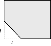
w and l are the dimension of the cover by Schaer and Wetzel (fig. 1)

s and t are the side lengths by Furedi and Wetzel (fig. 1)

m is the slope t/s

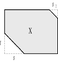
s2 is the side length in this work (fig. 2)

t2 is the side length in this work with the slope t2/s2=m

$\theta$ is the angle from slope m to X-axis

area is the area of this new cover

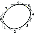
p1,p2,…,p8 are points with coordinates (xi,yi) (fig. 3) we set y2=0, y6=w, x8=0

arc is the polygonal closed arc

u[$\alpha$] is the unit vector of angle $\alpha$ (to X-axis)

Let s1,s2,…,s8 be the support lines of points p1,p2,…,p8 respectively. Their slopes are -m,0,m,$\infty$,-m,0,m,$\infty$ respectively.

u1,u3,u5,u7 are unit vectors pointing outward and perpendicular to s1,s3,s5,s7 respectively (fig. 3)

dist is the distant from (l,w) to the lower-left side of the new cover in fig. 3 (we can see this as the length of vector (l,w-t) in direction of u5)

dist2 is the distance from (0,0) to the upper-right side of the new cover in fig. 3 (we can see this as the length of vector (l,w-t2) in direction of -u1

out1R[xR,dis] is the condition that the length of vector p1-(xR,w) in direction of u1 is greater than dis (will be use to describe that p1 is going to escape the lower-left corner when the arc is justified right at x=xR)

out1L[xL,dis] is the condition that the length of vector p1-(xL+l,w) in direction of u1 is greater than dis (will be use to describe that p1 is going to escape the lower-left corner when the arc is justified left at x=xL)

out3L[xL,dis] is the condition that the length of vector p3-(xL,w) in direction of u3 is greater than dis

out3R[xR,dis] is the condition that the length of vector p3-(xR-l,w) in direction of u3 is greater than dis

out5L[xL,dis] is the condition that the length of vector p5-(xL,0) in direction of u5 is greater than dis

out5R[xR,dis] is the condition that the length of vector p5-(xR-l,0) in direction of u5 is greater than dis

out7R[xR,dis] is the condition that the length of vector p7-(xR,0) in direction of u7 is greater than dis

out7L[xL,dis] is the condition that the length of vector p7-(xL+l,0) in direction of u7 is greater than dis

bigout1L[xL] is the condition out1L[xL,dist] (equivalent to that p1 escapes the lower-left big corner when the arc is justified left at x=xL)

bigout1R[xR] is the condition out1R[xR,dist] (equivalent to that p1 escapes the lower-left big corner when the arc is justified right at x=xR)

Similarly for other bigoutkL/bigoutkR conditions.

smallout1L[xL] is the condition out1L[xL,dist2] (equivalent to that p1 escapes the lower-left small corner when the arc is justified left at x=xL)

smallout1R[xR] is equivalent to that p1 escapes the lower-left small corner when the arc is justified right at x=xR

Similarly for smalloutkL/smalloutkR conditions.

big1L is the condition that p1 escapes the big corner when justified left at x=0

big1R is the condition that p1 escapes the big corner when justified right at x=x4

Similarly for bigkL/bigkR conditions.

small1L is the condition that p1 escapes the small corner when justified left at x=0

small1R is the condition that p1 escapes the small corner when justified right at x=x4

Similarly, for smallkL/smallkR conditions.

Now wer mention the main conditions used in the article.

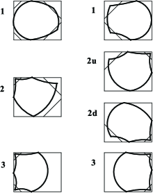
cond1L is big3L and big5L (upper left of fig. 9)
cond2L is big5L and small7L (middle left of fig. 9)
cond3L is small1L and small7L (lower left of fig. 9)
cond1R is big1R and big7R (upper right of fig. 9)
cond2uR is big7R and small5R (2u of fig. 9)
cond2dR is big1R and small3R (2d of fig. 9)
cond3R is small3R and small5R (lower right of fig. 9)

xL1 = (t2 - y1)/-m + x1 is the minimum x of the arc when justified to the lower-left small corner

xL7 = (w - t2 - y7)/m + x7 is the minimum x of the arc when justified to the upper-left small corner

xR5 = (w - t2 - y5)/-m + x5 is the maximum x of the arc when justified to the upper-right small corner

xR3 = (t2 - y3)/m + x3 is the maximum x of the arc when justified to the lower-right small corner

big1t3 is bigout1R[xR3]
big1t5 is bigout1R[xR5]
big3t1 is bigout3L[xL1]
big3t7 is bigout3L[xL7]
big5t1 is bigout5L[xL1]
big5t7 is bigout5L[xL7]
big7t3 is bigout7R[xR3]
big7t5 is bigout7R[xR5]

leftovert5 is that x8 $<$ xR5 - l
leftovert3 is that x8 $<$ xR3 - l
rightovert7 is that x4 $>$ xL7 + l
rightovert1 is that x4 $>$ xL1 + l

bigframeL[dx] is the drawing of 8-sided frame with big corners removed at x=dx on the left

bigframeR[dx] is the drawing of 8-sided frame with big corners removed at x=dx on the right

smallframk is the one with small corners removed

leftbigframe is bigframeL[0], justified left at x=0

rightbigframe is bigframeR[x4], justified right at x=x4

leftsmallframe is smallframeL[0]

rightsmallframe is smallframeR[x4]

From the article, we translate conditions as follows

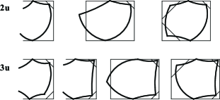
For additional conditions in fig. 10,

In the upper row, .2u: xR=xR5, .2uL: x8¡xL, .2uC: OUT1 and OUT7
In the bottom row, .3u: xR=xR3, .3uL: x8¡xL, .3uC: OUT7

Hence we have a similar additional conditions as follows.

.2d: xR=xR3, .2dL: x8¡xL, .2dC: OUT1 and OUT7
.3d: xR=xR5, .3dL: x8¡xL, .3dC: OUT1

Thus the conditions are as follows

1.: cond1L
2.: cond2L
2C.: cond2L, big3t7, big5t7
2R.: cond2L, rightovert7
3.: cond3L
3C. : cond3L, big3t7, big5t7
.2uC : cond2uR, big1t5, big7t5
.2uL : cond2uR, leftovert5
.2d : cond2dR
.3C : cond3R, big1t5, big7t5, smallout5R[xR3], big7t3
.3LC : cond3R, leftovert5, smallout5R[xR3], big7t3
.3LL : cond3R, leftovert5, smallout5R[xR3], leftovert3
.3u : cond3R, rightovert7
.3uC : cond3R, big7t3
.3uL : cond3R, leftovert3
.3d : cond3R, rightovert7
.3dC : cond3R, big1t5
.3dL : cond3R, leftovert5

Now we get into each case and subcase with some redundant conditions omitted in ().

1.2uC: cond1L, cond2uR, big1t5 (big7t5)
1.2uL: cond1L, cond2uR, leftovert5
1.3C: cond1L, cond3R, big1t5, big7t5, smallout5R[xR3], big7t3
1.3LC: cond1L, cond3R, leftovert5, smallout5R[xR3], big7t3
1.3LL: cond1L, cond3R, leftovert5, smallout5R[xR3], leftovert3
2C.2uC: cond2L, cond2uR, big3t7 (big5t7), big1t5 (big7t5)
2C.2uL: cond2L, cond2uR, big3t7 (big5t7), leftovert5
2R.2uL: cond2L, cond2uR, rightovert7, leftovert5
2.2d: cond2L, cond2dR
2C.3uC: cond2L, cond3R, big3t7 (big5t7), big1t5, big7t5
2.3uL: cond2L, cond3R, leftovert5, x5 $\leq$ x4
2R.3u: cond2L, cond3R, rightovert7, y7 $\leq$ y6
2C.3dC: cond2L, cond3R, big3t7 (big5t7), big1t3, big7t3
2.3dL: cond2L, cond3R, leftovert3, x3 $\leq$ x4
2R.3d: cond2L, cond3R, rightovert7, y7 $\leq$ y6
3C.3uC: cond3L, cond3R, big3t7, big5t7, big1t5, big7t5
3.3uL: cond3L, cond3R, leftovert5, x5 $\leq$ x4
3C.3dC: cond3L, cond3R, big3t7, big5t7, big1t3, big7t3
3.3dL: cond3L, cond3R, leftovert3, x3 $\leq$ x4

Note that some necessary condtions on xi and yi are used. When we omit some conditions, the minimum is even smaller (but still greater than 1.00001). The optimization is of the type called convex programming.

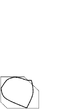
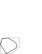
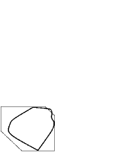
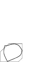
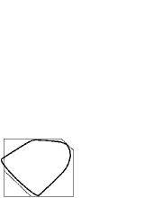
In each case, the output is the minimum length of the critical arc and drawing of the arc when justified to sides of the new cover. The minimum values are as follows (by Mathematica 7.0 and for later versions the result are just a bit different).

1.2uC: 1.02231
1.2uL: 1.001
1.3C: 1.00852
1.3LC: 1.00994
1.3LL: 1.04008
2C.2uC: 1.0093
2C.2uL: 1.01069
2R.2uL: 1.03344
2.2d: 1.00584
2C.3uC: 1.00596
2.3uL: 1.00318
2R.3u: 1.00392
2C.3dC: 1.00854
2.3dL: 1.00504
2R.3d: 1.00392
3C.3uC: 1.00001 (also ¿1.00001 by Mathematica version 11)
3.3uL: 1.05382
3C.3dC: 1.00001 (also ¿1.00001 by Mathematica version 11)
3.3dL: 1.05367