On the origin of two X-class flares in active region NOAA 12673

Flare-prolific active region NOAA 12673 produced consecutive X2.2 and X9.3 flares on 6 September 2017. To scrutinize the morphological, magnetic, and horizontal flow properties associated with these flares, a 7-hour time-series was used consisting of continuum images, line-of-sight/vector magnetograms, and 1600 Å UV images. These data were acquired with the Helioseismic and Magnetic Imager (HMI) and the Atmospheric Imaging Assembly (AIA). The white-light flare emission differed for both flares, while the X2.2 flare displayed localized, confined flare kernels, the X9.3 flare exhibited a two-ribbon structure. In contrast, the excess UV emission exhibited a similar structure for both flares, but with larger areal extent for the X9.3 flare. These two flares represented a scenario, where the first confined flare acted as precursor, setting up the stage for the more extended flare. Difference maps for continuum and magnetograms revealed locations of significant changes, i.e., penumbral decay and umbral strengthening. The curved magnetic polarity inversion line in the $\delta$-spot was the fulcrum of most changes. Horizontal proper motions were computed using the differential affine velocity estimator for vector magnetograms (DAVE4VM). Persistent flow features included (1) strong shear flows along the polarity inversion line, where the negative, parasitic polarity tried to bypass the majority, positive-polarity part of the $\delta$-spot in the north, (2) a group of positive-polarity spots, which moved around the $\delta$-spot in the south, moving away from the $\delta$-spot with significant horizontal flow speeds, and (3) intense moat flows partially surrounding the penumbra of several sunspots, which became weaker in regions with penumbral decay. The enhanced flare activity has its origin in the head-on collision of newly emerging flux with an already existing regular, $\alpha$-spot. Umbral cores of emerging bipoles were incorporated in its penumbra, creating a $\delta$-configuration with an extended polarity inversion line, as the parasitic umbral cores were stretched while circumventing the majority polarity.

1 Introduction

The relationship between sunspot numbers and flare occurrence as a function of the solar cycle was extensively examined, revealing a surge of renewed solar activity occurs a few years after the cycle maximum (Fritzová-Švestková & Švestka, 1973; Švestka, 1995). Temmer et al. (2003) noticed, in a correlation analysis of flare occurrence and sunspot number, that the flare occurrence lags behind the sunspot number. For solar cycle 23, Bai (2006) found high flare activity in the late declining phase of the cycle. Not only an increased flare activity was noted but many low-latitude coronal holes were repeatedly observed during the declining and minimum phases of solar cycle 23 (Abramenko et al., 2010). In addition, Gopalswamy et al. (2003) determined that the occurrence rate of coronal mass ejections (CMEs) peaked two years after the cycle maximum, and in the analysis of Kilcik et al. (2011), the maximum speeds of CMEs also peaked approximately at that time. Recently, Lee et al. (2016) reported that the occurrence rates of major flares and front-side halo CMEs are higher during the descending phase of solar cycle 23 as compared to other phases of the cycle. The recent rejuvenation in the Sun’s large-scale magnetic field during solar cycle 24 starting in the second half of 2014, was pointed out by Sheeley & Wang (2015). They concluded that this was the result of systematic flux emergence in active regions, whose longitudinal distribution greatly increased the Sun’s dipole moment.

The role of horizontal shear flows in building up magnetic stress in flare-productive active regions was already noticed by Harvey & Harvey (1976). Horizontal shear flows are not only responsible for magnetic stress but are also drivers for magnetic reconnection (Yurchyshyn et al., 2006). Yang et al. (2004) measured the horizontal flows in active region NOAA 10486 before an X10 flare and found shear flows with local correlation tracking (LCT, November & Simon, 1988) of up to 1.6 km s^-1 along the polarity inversion line (PIL). These strong shear flows were correlated with white-light flare kernels in the optical range. Strong horizontal shear flows, which decrease with height in the atmosphere, were also observed by Deng et al. (2006) in the same active region. Based on photospheric flows and the flux around the PIL, Welsch et al. (2009) derived indicators for the occurrence of flares. Many case studies established crucial links between photospheric shear flows, build-up of free-energy in a stressed magnetic field topology, and major flares (e.g., Tan et al., 2009; Liu et al., 2010). More recently, Beauregard et al. (2012) and Wang et al. (2014) analyzed the horizontal flows in active region NOAA 11158 in relation to an X2.2 flare. The photospheric signatures produced by this major flare were rather diminutive. On the other hand, during the impulsive phase shear flows around the PIL showed a sudden decrease and a change in the intrinsic rotation of the two main sunspots. Recently, Wang & Liu (2015) reviewed shear motions, sunspot rotation, and flux emergence regarding their role in triggering solar eruptive events.

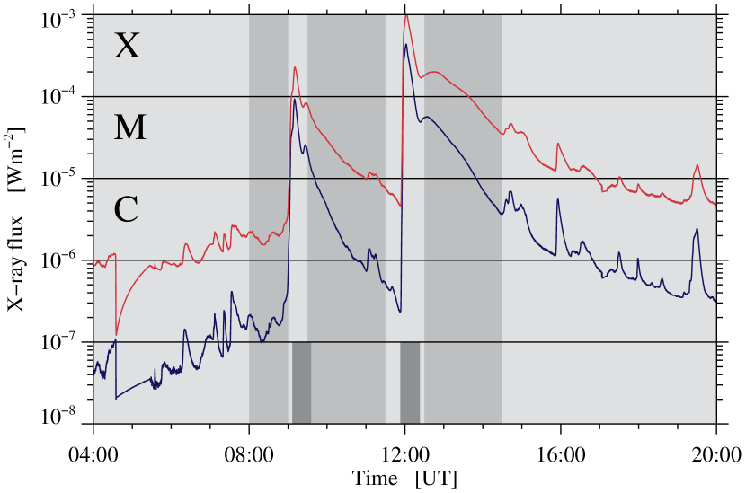
Figure 1: GOES 13 X-ray flux on 6 September 2017 in the 0.1– 0.8 nm (top) and 0.05 – 0.4 nm (bottom) energy channels. The three light gray regions indicate the pre-flare, interim, and post-flare phases, which were used to compute horizontal proper motions (Fig. 4). The two narrow, dark gray regions refer to the time intervals for computing the white-light flare kernels (Fig. 2).

2 Observations and data reduction

Active region NOAA 12673 appeared on the South-East limb of the solar disk on 29 August 2017 as a simple $\alpha$-spot. Over the next few days, it maintained its single-spot configuration. On 3 September 2017, new flux emerged as bipolar regions following the $\alpha$-spot, and by the next day, the region had acquired a complex $\beta\gamma$-configuration, when the positive polarity of the bipoles merged with the main spot. The complexity of the region increased, and a $\delta$-configuration appeared by 5 September 2017, when the negative polarity of the bipoles collided head-on with the main spot. A unique aspect of this flare-prolific active region was the short period of just three hours between two major flares. The X2.2 flare occurred at 08:57 UT followed by an X9.3 flare at 11:53 UT on 6 September (Fig. 1). The latter was the strongest flare in solar cycle 24. A detailed description of the magnetic evolution is given by Yang et al. (2017), Sun & Norton (2017) call attention to an overall extremely high flux emergence rate and non-potential magnetic field topology, and Wang et al. (2018) report extremely strong transverse magnetic fields near the PIL of more than 5500 G.

The present work is based on HMI continuum images and magnetograms (Scherrer et al., 2012) and UV images obtained by AIA (Lemen et al., 2012), both on board the Solar Dynamics Observatory (SDO, Pesnell et al., 2012). These time-series cover a 7-hour period from 08:00 –15:00 UT. The data were divided in three sets: “pre-flare” one hour before the X2.2 flare (08:00 – 09:00 UT), “interim” two hours between the two X-class flares (9:30 –11:30 UT), and “post-flare” two hours after the X9.3 flare (12:00 –14:00 UT). The goal was to capture differences in the flow fields before, in between, and after the two major flares. The HMI and AIA data had a cadence of 45 s and 48 s, respectively, and the former were adapted to the AIA image scale of 0.6″ pixel^-1. Images and magnetograms were then compensated for differential rotation and rotated to the position, when the active region crossed the central meridian at 19:00 UT on 3 September 2017. The continuum and UV images were corrected for the center-to-limb variation and divided by a 2D limb-darkening function based on the average quiet-Sun intensity.

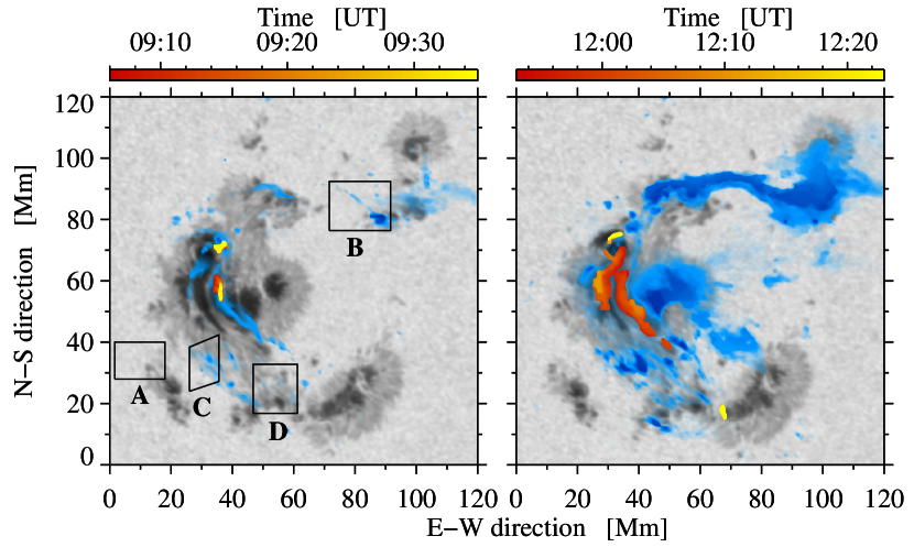
Figure 2: Continuum images at 08:57 UT (left) and 11:53 UT (right) superimposed with the white-light flare kernels derived from 30-minute time-series of continuum images covering the X2.2 and X9.3 flares (see scale bar for the temporal evolution). The blue-colored overlays represent the 2D frequency distribution of pixels exhibiting strong UV excess brightenings with respect to the pre-flare phase. The boxes mark the locations of penumbral decay (A – C) and umbral strengthening (D).

For tracking the plasma flows we used the Space-weather HMI Active Region Patches (SHARP) vector magnetogram data product with 12-minute cadence (Bobra et al., 2014). The SHARP maps were generated from polarization measurements at six wavelengths along the Fe i 6173 Å spectral line (Hoeksema et al., 2014). The data were inverted using the Very Fast Inversion of the Stokes Vector (VFISV) algorithm (Borrero et al., 2011) based on the Milne-Eddington approximation, and the 180^∘ ambiguity in azimuth was resolved using the minimum-energy code (Metcalf, 1994; Leka et al., 2009). The inversion provided several physical parameters, including maps of continuum intensity, magnetic field, azimuth, inclination, and line-of-sight (LOS) velocity (see online movie). Since only six wavelength points are used in the inversion of HMI vector magnetograms the errors are usually large in the derived magnetic field parameters. In addition, an upper limit of 5000 G is set for the magnetic field strength. The total magnetic field strength and transverse magnetic field in all 36 maps combined exceed 4000 G only for about 2100 and 250 pixels, respectively. Thus, extremely strong magnetic fields, as reported by Wang et al. (2018), were not observed. From the two types of available SHARP data products (Bobra et al., 2014), definitive maps were only available for the interim and post-flare phases because of a semiannual spacecraft eclipse period. Thus, five near-real-time maps were used for the pre-flare phase.

In the next step, images and magnetic field maps were corrected for geometrical foreshortening (Verma & Denker, 2011), which resulted in maps, where one pixel corresponds to 400 km $\times$ 400 km. Horizontal proper motions were derived with DAVE4VM (Schuck, 2008) using convolution with the Scharr operator and a five-point-stencil with a time difference of 12 min between neighboring magnetograms for the spatial and temporal derivatives of the magnetic field, respectively. The horizontal velocities were averaged over one hour for the pre-flare period, and two hours for the interim and post-flare periods.

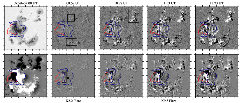
Figure 3: One-hour averaged continuum image (top-left) and magnetogram (bottom-left) of active region NOAA 12673. The next four panels (top and bottom) covering an area of 120 Mm $\times$ 120 Mm show difference maps scaled between $\pm 0.2$ $I_{0}$ (continuum images) and $\pm 500$ G (magnetograms). The red and blue contours mark the boundaries of negative and positive polarities comprising the $\delta$-spot. The intersection of these two colored lines demarcates the PIL. The boxes labeled ‘a’, ‘b’, ‘c’, and ‘d’ mark locations of persistent changes.

3 Results

Active region NOAA 12673 produced many C-, 27 M-, and four X-class flares in one week (4 –10 September 2017). The two X-class flares on 6 September 2017 were separated in time by only about three hours (Fig. 1). The immediate succession of two major flares motivated this case study. The flare kernels for both flares were identified in continuum and UV images. To extract the photospheric continuum emission, average maps were created using 40 continuum images before 09:06 UT and 11:53 UT for the X2.2 and X9.3 flares, respectively. These background maps were subtracted from individual images covering the next 30 min starting at the flare initiation time. Choosing a threshold of $+0.1\,I_{0}$, where $I_{0}$ is the quiet-Sun intensity, for the excess intensity was sufficient to unveil the continuum flare emission and its location. To obtain the areal extent with sub-pixel accuracy, the images were magnified by a factor of 2.5 using Fourier interpolation. Small-scale features were discarded and smooth boundaries were ensured using morphological opening. The temporal evolution of regions with continuum flare emission is given by the scale bars in Fig. 2, where red shows the beginning and yellow the end of the white-light flare.

An average map based on 50 images taken between 07:30 –08:10 UT was used to compute the excess UV emission after both flares. This background map was then subtracted from all individual images over a two-hour period in both the interim and the post-flare phases. The flare ribbons and kernels are characterized by very strong UV emission. Thus, a threshold of 3.5 times the background emission was used to label the flaring regions. A 2D frequency distribution of areas displaying significant UV excess brightenings was superimposed in blue colors on the gray-scale continuum image in both panels of Fig. 2. Therefore, a strong saturation of the color blue indicates regions, which exhibit the strongest UV flare emissions.

During the X2.2 flare, the white-light flare kernels were confined and limited to two small patches near the PIL in the positive polarity of the $\delta$-spot. These kernels appeared almost 10-min after the flare peak time. In contrast, the white-light kernels for the X9.3 flare appeared 3 min after the X-ray emission peaked. They were more extended and formed a two-ribbon configuration on both sides of the PIL. These two ribbons migrated away from the PIL as indicated by the color gradient from dark red to light orange in the right panel of Fig. 2. Two remote brightenings (yellow) appeared at the periphery of two umbral cores away from the PIL towards the end of the 30-minute interval. The excess UV emission for the X2.2 flare was mainly limited to the $\delta$-spot and was sparsely seen in neighboring sunspots. However, for the X9.3 flare, the flaring area was much larger, and the excess emission stretched to all sunspots in the active region. Even though both X-class flares can be categorized as homologous flares, significant differences in their morphology and temporal evolution are apparent, both for the white-light flare kernels and the excess UV brightenings. The X2.2 flare likely weakened the magnetic topology facilitating the next eruptive flare. Following the evolution in time-lapse movies of the Large-Angle Spectrometric Coronagraph (LASCO, Brueckner et al., 1995), a CME erupted only for the X9.3 flare, whereas the X2.2 flare stayed confined.

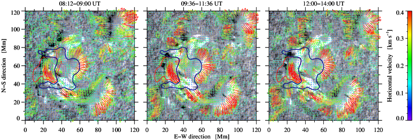
Figure 4: Time-averaged horizontal proper motions in active region NOAA 12673 computed with DAVE4VM for the pre-flare, interim, and post-flare phases (left-to-right). Color-coded vectors indicate magnitude and direction of the horizontal flows. The background images are LOS velocity maps based on spectral inversions at 08:36 UT, 10:36 UT, and 11:00 UT scaled between $\pm 1.4$ km s^-1 (black/white corresponds to blue/redshifts).

Active region NOAA 12673 contained four major sunspots. The large, central $\delta$-spot was the fulcrum of all flare activity. This spot differed from typical $\delta$-spots and was formed by the head-on collision of newly emerging bipolar regions with pre-existing flux in the form of a simple $\alpha$-spot. This created a complex active region (Yang et al., 2017) with the main spot containing the $\delta$-configuration and three neighboring spots, i.e., two on top (‘c’ and ‘d’ in Fig. 2) and spot ‘b’ at the bottom, which also exhibited peculiar proper motions. Within the $\delta$-spot a curved light-bridge ‘a’ coincides with the PIL. The umbral cores on both sides of the light-bridge are elongated and curved, which already provides a first indication of shear flows and twist within the flux system. This magnetically “stressed” configuration motivated this study, and difference maps were computed for both continuum images and magnetograms (Fig. 3) to clearly identify, where the major changes occurred during and after the major flares.

The difference maps were computed by subtracting time-averaged maps from individual continuum images and magnetograms. Before the X2.2 flare only minute changes occurred in both continuum intensity and magnetic field, with some strengthening of the magnetic field in the upper part of the PIL. Starting with the X2.2 flare, these changes became more apparent in this location, where the reduced/strengthened magnetic fields in positive/negative polarities across the PIL appeared as an X-shaped feature. One and a half hours after the X2.2 flare, considerable changes took place in the vicinity of the PIL. A small dark localized region at coordinates (25 Mm, 50 Mm) appeared in both types of difference maps in the negative polarity of the $\delta$-spot. This is caused by the parasitic polarity trying to bypass the dominant positive polarity of the $\delta$-spot, which leads to flux cancellation. The top of the PIL retained the reduced magnetic field. At this time, prominent changes in intensity and magnetic field became evident in the neighboring sunspots ‘b’, ‘c’, and ‘d’ as well. In the positive-polarity spot ‘b’ and negative-polarity spots ‘c’ and ‘d’, the decay of the penumbra on the side facing the $\delta$-spot was evident in both difference maps. Umbral strengthening in the immediate vicinity of penumbral decay was seen in spots ‘b’ and ‘d’. During and after the X9.3 flare, the changes in all marked locations remained, which indicates that the magnetic topology of the active region reached a new equilibrium.

The regions A – C and D (as marked in Fig. 2) were chosen as examples for the regions exhibiting penumbral decay and umbral strengthening, respectively (Fig. 5). Aligned and geometrical corrected continuum images and total magnetic flux maps from the inverted vector magnetograms were used to compute the photometric and magnetic flux evolution in these regions. The penumbra and umbra were selected using the intensity threshold of $I_{\mathrm{pen}}<0.9\,I_{0}$ and $I_{\mathrm{umb}}<0.65\,I_{0}$, respectively, where $I_{0}$ refers to the normalized quiet-Sun intensity (see column two in the online movie). In region B, area and flux decayed after the X2.2 flare, whereas these values declined in region A only after the X9.3 flare. The penumbra decayed at first in region C after the X2.2 flare but in the interim phase, the penumbra replenished and later decayed after the second flare. In contrast, area and flux increased in umbral region D after both flares.

To quantify proper motions in and around the $\delta$-spot, we applied DAVE4VM to vector magnetograms (see Fig. 3). The time-series was divided into the three aforementioned flare phases. Only some of the flow features were persistent. Nonetheless, also these region were not static but continuously exhibited dynamic features in all phases: (1) The moat flows around negative polarity spot ‘d’, positive polarity spot ‘b’, and the western side of the $\delta$-spot – the moat flows in sunspot ‘d’ and the $\delta$-spot weakened from pre- to post-flare phase. (2) The pronounced flow pattern that leads to the separation of the negative polarity of the $\delta$-spot and the positive-polarity spot ‘b’ – the flow vectors in northward direction in the $\delta$-spot were well aligned with the PIL. In the interim phase, these flows appeared to form an inverted S tracing the shape of the PIL. These flows had almost identical values in the pre- and post-flare phases ($\bar{v}_{\mathrm{pre}}=0.49$ km s^-1 and $\bar{v}_{\mathrm{post}}=0.50$ km s^-1). The opposing southward flows in the southern sunspot became more curved with increased areal coverage from pre-flare to interim phase. These flows became somewhat stronger in the interim phase ($\bar{v}_{\mathrm{pre}}=0.35$ km s^-1 to $\bar{v}_{\mathrm{post}}=0.37$ km s^-1) and traced the circumventing motion of spot ‘b’ around the positive polarity of the $\delta$-spot. In general, the velocities along the PIL remained high during all three phases with some patches of velocities reaching 0.5 – 0.7 km s^-1. (3) The velocities in the positive part of the $\delta$-spot remained low. Weak curling flows exhibited counter-streaming along the upper part of the PIL with respect to the northward motion seen in the negative polarity of the $\delta$-spot. These flow vectors were seen prominently in the pre-flare and interim phases ($\bar{v}_{\mathrm{pre}}=0.21$ km s^-1 to $\bar{v}_{\mathrm{int}}=0.26$ km s^-1). However, uniform converging motions to the center replaced the curling motions in the post-flare phase.

The LOS velocity maps based on inversions provided the missing information to study flows around the $\delta$-spot in 3D. Only some of the flow features were persistent. The Evershed flow appears in the upper/lower sunspots and the positive polarity of the $\delta$-spot. Although, only two blueshifted patches can be seen in the negative-polarity $\delta$-spot. The flows parallel to the PIL displayed successive red/blue/redshifts. This alternating flow pattern remained persistent before, between, and after both flares.

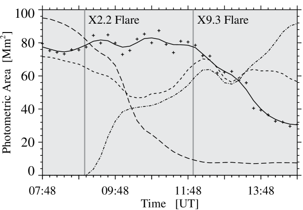
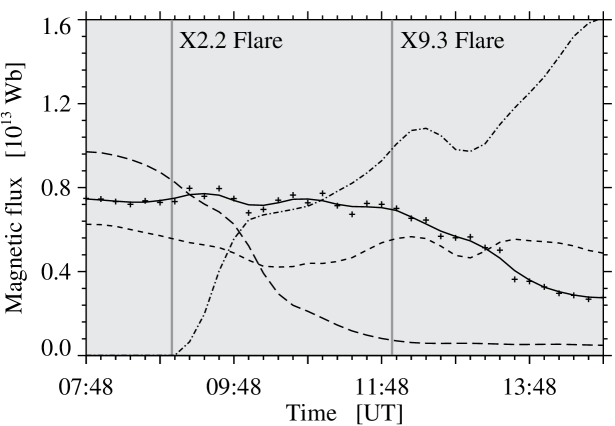
Figure 5: Evolution of photometric area and magnetic flux for the four regions A (solid), B (long-dashed), C (dashed), and D (dashed-dotted) over an 8-hour period on 6 September 2017. Regions A – C indicate penumbral decay, whereas D is a site of umbral strengthening. The time profiles were significantly smoothed to avoid clutter. The original data points are shown as plus signs for region A to give an impression of the scatter.

4 Discussion and conclusions

Peculiar horizontal proper motions are at the center of the present work, which were responsible for creating shear and twisting motions powering two X-class flares in declining phase of solar cycle 24. Zirin & Wang (1993) observed a large active region with convoluted magnetic fields along the PIL and with a large curl of the horizontal magnetic field. The field lines along the PIL reconnected with the expanding and stretched-out opposite-polarity regions. Similarly, the extended and curved PIL of the present $\delta$-spot was the site of many flares, specifically two major X-class flares, because of strong magnetic field gradients between drawn out umbral cores of opposite polarity in close proximity. Sudol & Harvey (2005) showed that abrupt, significant, and permanent changes of the photospheric longitudinal magnetic field are ubiquitous features of X-class flares, which were observed for the two X-class flares, too.

Persistent flow patterns along PIL contributed to sheared magnetic field structures: (1) Strong shear flows affected the negative, parasitic polarity, which was sliding along the PIL northward. (2) A group of positive-polarity spots bypassed the main spot to the south, and the separation speed increased after the two X-class flares. (3) Rapid penumbral decay weakened the moat flow associated with several sunspots surrounding the main spot.

Yang et al. (2017) proposed a “block-induced” eruption model for the X9.3 flare. Newly emerging flux is blocked by already existing flux, which leads to increased flare-productivity. In addition, they conclude that the X9.3 flare was triggered by an erupting filament due to kink instability. However, this flare scenario is not new. A similar flare-prolific active region NOAA 5395 was observed by Wang et al. (1991), which exhibited a complex structure, an extended PIL, coalescence of spots creating a $\delta$-configuration, expulsion of smaller spots in curved trajectories, and strong shear motions. Furthermore, Denker & Wang (1998) noticed a similar phenomenon on much smaller scales, i.e., the head-on collision of flux systems forming a small $\delta$-spot, which produced many C- and M-class flares. Tanaka (1991) studied a similar $\delta$-spot with complex structure and consecutive flares along the PIL. The $\delta$-spot was formed by compressing and compacting opposite polarities. In addition, a light-bridge coincided with the PIL with strong horizontal motions. The author proposed that flares in evolving $\delta$-spots are caused by the emergence of twisted magnetic flux ropes. The magnetic topology of such regions is governed by tightly twisted (sheet-like) magnetic knots within emerging flux ropes. The elevated flare productivity of such regions is likely the result of internal magnetic structure and formation of anomalous magnetic ropes.

Active region NOAA 12673 started out as a simple $\alpha$-spot. The emergence of multiple bipolar regions to the north and south created a complex active region, when first the leading spots of the same polarity as the $\alpha$-spot were incorporated in the already existing flux system. The $\delta$-configuration was created when the trailing polarity piled up behind the main spot. This $\delta$-spot is different than usual $\delta$-configurations because the PIL is established within the remnants of the compacted bipolar regions. The parasitic polarity is surrounded on three sides by the majority polarity, and it is the northern side, where the extended and curved umbral cores circumnavigate the pre-existing flux system that initiates the flare. This location is also the site of white-light flare emission in both flares. The observed photospheric shear motions created a highly non-potential field configuration, which provided the energy that powered these, in many aspects homologous, X-class flares (e.g., Harvey & Harvey, 1976; Yang et al., 2004). However, differences exist, with the former flare being more confined and the later being related to a filament eruption and major CME. The emergence of new flux plays a role in the onset of flares. Wang et al. (1994) studied five X-class flares and noticed that the magnetic shear along the PIL increased after all flares. According to authors, the emergence of new flux at the onset of each flare had sufficient energy to power flares and left the photosphere in a more sheared configuration.

The white-light brightenings associated with two X-class flares are similar to those in a case study of Wang et al. (2017), who found low-atmospheric small-scale precursors, i.e., brightenings along the PIL before an M6.5 flare. These brightenings moved along the PIL instead of away and were confined, while the main flare was much more extended, as in the flare model proposed by Kusano et al. (2012). In this model, the pre-flare brightenings can be ascribed to heating of the current sheet between the pre-existing large-scale field and small-scale intrusions of parasitic polarity forming barb-like structures along the PIL. This interaction aided the reconnection of the ambient legs of large-scale sheared loops rooted in major flux concentration, thus producing precursor brightenings. The X2.2 and X9.3 flares may not completely follow this scenario, but the similarity arises from small-scale brigthenings appearing along the PIL during the confined X2.2 flare, followed by more extended flare emission in the X9.3 flare, which was associated with a filament eruption and a CME.

Appendix A Online material

Online movie 1: Results of the spectral inversions for the photospheric Fe i 6173 Å line. This snapshot shows physical maps of active region NOAA 12673 at 11:48 UT on 6 September 2017 just before the X9.3 flare. The whole time-series consists of 35 maps at a 12-minute cadence starting at 07:48 UT: normalized intensity $I/I_{0}$, masks of penumbra (gray) and umbra (black), horizontal component of the magnetic flux density $B_{\mathrm{hor}}$, LOS velocity $v_{\mathrm{LOS}}$, vertical component of the magnetic flux density $B_{\mathrm{z}}$, and total flux density (top-left to bottom-right).