Modeling ringdown II. Aligned-spin binary black holes, implications for data analysis and fundamental theory

Abstract

The aftermath of binary black hole coalescence is a perturbed remnant whose gravitational radiation rings down, encoding information about the new black hole’s recent history and current state. It is expected that this ringdown radiation will be composed primarily of Kerr quasinormal modes, and thereby enable tests of general relativity. Here, the first complete ringdown signal model for nonprecessing binary black hole systems is presented: multipole amplitudes and phases are modeled as functions of initial binary parameters. It is found that using the peak time of the dominant merger multipole as a reference results in the dominant mode’s excitation being a remarkably simple linear function of system parameters, strongly suggesting that an analytic treatment may be within reach. In particular, for initially nonspinning black holes, the dominant quadrupole is excited as $-4$ times the system’s symmetric mass ratio. Application of the model to parameter estimation allows general relativity predictions for mode amplitudes independently of signal strength. Treatment of GW150914 indicates some mode amplitudes and relative phases are intrinsically difficult to constrain.

I Introduction

Direct detections of gravitational waves by LIGO and Virgo bring the possibility of testing general relativity’s (GR’s) detailed predictions Abbott et al. (2017a, b, 2016a); Yunes et al. (2016); Abbott et al. (2016b). With prospective detectors such as LIGO-India Unnikrishnan (2013), KAGRA Kanda et al. (2017), Einstein Telescope (ET) Maselli et al. (2017) and LISA Tang et al. (2018), it is likely that there will be many high signal-to-noise ratio (SNR) detections, allowing for increasingly stringent tests of GR Bhagwat et al. (2016); Baibhav et al. (2018); Berti et al. (2016); Yang et al. (2017); Cabero et al. (2018). To this end, the final moments of binary black hole coalescence are of particular interest. Shortly after two black holes (BHs) merge, the remnant is expected to be a perturbed BH whose gravitational radiation rings down with frequencies predicted by Teukolsky’s equations Leaver and Chandrasekhar (1985); Teukolsky (1972). In particular, classical linear perturbations of the Kerr spacetime induce transient radiative quasinormal modes (QNMs) that are exponentially damped and oscillatoryNollert and Price (1999); Kokkotas and Schmidt (1999); Berti et al. (2009). The damped ringing of these modes is colloquially named ringdown Nollert and Price (1999).

It is expected that the spatiotemporal dependence of each QNM is determined by the remnant’s mass and spin, which in turn determine the matter-free background metric (e.g. Gürlebeck (2015)). Consequently, direct observation of two or more QNMs has been linked to testing the no-hair hypothesis Gossan et al. (2012); Meidam et al. (2014); Berti et al. (2006).

However, significant challenges must first be overcome. Accurate and physically parametrized signal models are needed to interface theory with experiment. Despite the development of post-Newtonian (PN) theory to map initial binary parameters to gravitational waves for the early inspiral, there is no equivalent analytic theory developed for BH ringdown Berti et al. (2009). As a result, numerical relativity (NR) simulations have been used to provide QNM amplitudes and their relative phases where BH perturbation theory only provides the QNM’s spatiotemporal functions Kamaretsos et al. (2012a); Buonanno et al. (2007); Berti et al. (2007); London et al. (2014); McWilliams (2019). Concurrently, signal models for binary black hole (BBH) inspiral, merger and ringdown, are often limited by their subdominant harmonic content London et al. (2018); Cotesta et al. (2018), or are not readily parametrizable for deviations from BH perturbation theory’s predictions Varma et al. (2019).

Figure 1: The choice of time origin, $\hat{t}_{\mathrm{ref}}$, affects ringdown amplitude values independently of ringdown’s beginning at $t=T_{\mathrm{start}}$. Top panel: Result of NR simulation of 1.2:1 mass ratio BBH with nonspinning progenitors. The gravitational wave strain is shown at an orientation of $(\theta,\phi)=(14\pi/5,0)$. Thick grey curves show its envelope, and vertical dotted lines mark two choices for reference time. Bottom panel: the effect of reference time on the dominant QNM amplitude, $\mathcal{A}_{220}$, as a function of symmetric mass ratio, $\eta=M_{1}M_{2}/M^{2}$. Dashed grey curves show the effect of varying $\hat{t}_{\mathrm{ref}}$ between $-25\leavevmode\nobreak\ M$ and $25\leavevmode\nobreak\ M$ in steps of $5\leavevmode\nobreak\ M$ relative to peak strain. Curves shown are approximately linear. The use of $\hat{t}_{\mathrm{ref}}^{(a)}$ yields the red curve as used in e.g. Ref. Gossan et al. (2012). Use of $\hat{t}_{\mathrm{ref}}^{(b)}$ (blue) has the particular effect of normalizing the QNM amplitude to unity when $\eta=0.25$ (i.e. an equal mass binary ).

In this work, the first detailed signal model for QNM excitations (amplitudes and phases) of spinning but nonprecessing BH binaries is presented. This work is the sequel to, Ref. London et al. (2014), which only explores BBHs with nonspinning progenitors. Because this signal model presented here outputs the expected ringdown radiation of nonprecessing BBH systems, we will refer to it as RDNP. RDNP’s construction and output shed new light on the potential development of a PN-like theory for BH ringdown. For the first time, RDNP shows that non-monotonic excitations and abrupt transitions in relative phase are robust features of the nonprecessing BBH parameter space. Its primary use is expected to be in testing GR during and after LIGO’s third observing run (O3) Meidam et al. (2014); Gossan et al. (2012); Cabero et al. (2018); Yang et al. (2017); Carullo et al. (2018, 2019). While there is a focus here on ground based detectors, the primary results of this work apply to proposed space based detectors such as LISA Berti et al. (2006).

Figure 2: Construction and validation of RDNP: (Left) 2D surface plot comparing calibration points (colored circles) to model fit (smooth gradient) for $|A_{2220}|$. Values of calibration points differ from model fit if adjacent colors differ. BAM validation waveforms are marked with x. (Center) 2D surface plot for the intrinsic phase $\arg(A_{3230})$. Here, $\delta$ is explicitly considered to be a function of $\eta$. (Right) Average matches as a function of source inclination for select noncalibration simulations including all multipoles with $\ell\leq 5$. Each case has a total system mass of $100\leavevmode\nobreak\ M_{\odot}$. A sample precessing system (red circles, label “q1.2_p”) having $(\chi^{(1)}_{x},\chi^{(1)}_{y},\chi^{(1)}_{z})=(0.3844,-0.1346,-0.1189)$ and $(\chi^{(2)}_{x},\chi^{(2)}_{y},\chi^{(2)}_{z})=(-0.3536,0.2181,0.0861)$ is shown in addition to 4 nonprecessing cases.

II Numerical Relativity Simulations

Using 101 nonprecessing simulations from the Georgia Tech catalog, strain QNM amplitudes are calculated and then modeled in geometric units ($M=G=c=1$) Jani et al. (2016). Among the simulations used, 42 are nonspinning, 31 have different dimensionless spins on each BH, and 28 have equal spin on each BH. Mass ratios vary between 1:1 and 1:15, and component spins vary between -0.8 and 0.8. Seven simulations (six nonprecessing and one precessing) from the BAM code are used for model validation Brügmann et al. (2008a); Husa et al. (2008).

III Ringdown Start

This section reviews the data processing choices used to define ringdown within simulations of merging BBHs. Briefly, the connection between observable gravitational wave strain, and the output of NR simulations is discussed. More importantly, the impact of the extrinsically chosen ringdown start time on ringdown amplitudes is reviewed. A choice that simplifies the behavior of the dominant quadrupole amplitude is presented.

Given the gravitational wave strain, $h=h_{+}-ih_{\times}$, where $h_{+}$ and $h_{\times}$ are the observable gravitational wave polarizations, a multipolar representation convenient for NR uses the spherical harmonics of spin weight $-2$  Ruiz et al. (2008)

$$r\,h_{\bar{\ell}\bar{m}}(t) ={\int_{\Omega}}{{}_{-2}}Y_{\bar{\ell}\bar{m}}^{*}(\theta,\phi)h(t,\theta,\phi)\,\mathrm{d}\Omega\;.$$ (1)

Concurrently, BH perturbation theory confers that strain is naturally represented as a sum over the physical system’s eigenmodes

$$r\,h(t,\theta,\phi)\approx\sum_{\ell mn}\,{{}_{-2}}S_{\ell mn}(\theta,\phi)\,\mathcal{A}_{\ell mn}e^{i\tilde{\omega}_{\ell\bar{m}n}t}\;,$$ (2)

where $\ell\geq 2$, $|m|\leq\ell$, and $n\geq 0$. In Equation (1), $r$ is the source’s luminosity distance and $*$ denotes complex conjugation. In Equation (2), ${{}_{-2}}S_{\ell mn}(\theta,\phi)$ is a spheroidal harmonic function, $\tilde{\omega}_{\ell\bar{m}n}=\omega_{\ell\bar{m}n}+i/\tau_{\ell\bar{m}n}$ is the QNM’s complex ringdown frequency, $n$ is an overtone index, and $\mathcal{A}_{\ell mn}$ is the QNM excitation amplitude Leaver and Chandrasekhar (1985); Berti et al. (2009). In principle, Equation (2) is approximate as other possible contributions to the radiation, such as power-law tails, are not included. However, this work focuses on the regime in which QNM decay dominates Teukolsky (1972); London et al. (2014). Thus, in practice, the QNM representation is considered to be exact when the start of ringdown is appropriately chosen, and the self-consistency of this picture well established London et al. (2014); Kelly and Baker (2013).

The combination of Eqs. (1)-(2) yields that Equation (1)’s spherical harmonic multipole moments are sums over Equation (2)’s eigenmodes Press and Teukolsky (1973); London et al. (2014)

$$r\,h_{\bar{\ell}\bar{m}}=\sum_{\ell n}A_{\bar{\ell}\bar{m}\ell n}e^{i\tilde{\omega}_{\ell\bar{m}n}t}\;.$$ (3)

In Equation (3), we have used Eqs. (1)-(2) along with the orthogonality of spherical and spheroidal harmonics in $m$. Moreover, an effective QNM amplitude $A_{\bar{\ell}\bar{m}\ell n}$, and a time coordinate, $t$, are defined as

$$A_{\bar{\ell}\bar{m}\ell n}=\sigma_{\bar{\ell}\bar{m}\ell\bar{m}n}\,\mathcal{A}_{\ell\bar{m}n}\text{, and }\;t=\hat{t}-\hat{t}_{\mathrm{ref}}\,,$$ (4)

where in Equation (4), $\sigma_{\bar{\ell}\bar{m}\ell\bar{m}n}$ are the mixing coefficients between spherical and spheroidal harmonics Berti and Klein (2014); London and Fauchon-Jones (2019), and $\hat{t}$ is an observer’s time coordinate.

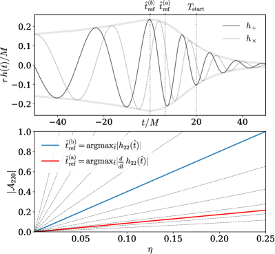
Three conventions are used to practically define the ringdown region and assist model construction. First, we note that different choices of reference time, $\hat{t}_{\mathrm{ref}}$, result in different values of $A_{\bar{\ell}\bar{m}\ell n}$ for different BBH configurations. That is, when comparing two such conventions, for example, $\hat{t}_{\mathrm{ref}}^{(a)}$, defined at the peak of $|\frac{d}{dt}{h}_{22}|$ (as in Refs. Kamaretsos et al. (2012b); Gossan et al. (2012)), and $\hat{t}_{\mathrm{ref}}^{(b)}$ defined at the peak of $h_{22}$ (as is used here), the resulting values of $A_{\bar{\ell}\bar{m}\ell n}$ differ according to

$$A_{\bar{\ell}\bar{m}\ell n}^{(a)}/A_{\bar{\ell}\bar{m}\ell n}^{(b)}\;\;\propto\;\;e^{\,i\tilde{\omega}_{\ell\bar{m}n}(\;\hat{t}_{\mathrm{ref}}^{(b)}\,-\,\hat{t}_{\mathrm{ref}}^{(a)}\;)\,}.$$ (5)

As the QNM frequencies and decay times depend nontrivially on the initial BH masses and spins, Equation (5) communicates that different conventions for $\hat{t}_{\mathrm{ref}}$ generally result in different pictures of QNM excitation. Figure 1 illustrates the effect for the dominant QNM amplitude, $\mathcal{A}_{220}$, on the space of initially nonspinning BBHs with masses $M_{1}$ and $M_{2}$, with a symmetric mass ratio, $\eta=M_{1}M_{2}/(M_{1}+M_{2})^{2}$. Note that $\sigma_{22220}\approx 1$ for all remnant BH spins, thus $\mathcal{A}_{220}\approx A_{2220}$ Berti and Klein (2014); London and Fauchon-Jones (2019). Here, not only does the choice of $\hat{t}_{\mathrm{ref}}$ affect $\mathcal{A}_{220}$’s functional form, but $\hat{t}_{\mathrm{ref}}^{(b)}$ (at peak $h_{22}$) is revealed to be a remarkably simple choice, one resulting in $|\mathcal{A}_{220}|\approx 4\eta$. For this reason, $\hat{t}_{\mathrm{ref}}=\hat{t}_{\mathrm{ref}}^{(b)}$ is used here.

Second, we note that throughout the nonspinning BBH parameter space, system mass and angular momentum typically continue to evolve prior to $t\approx 16\leavevmode\nobreak\ M$, and are constant thereafter Buonanno et al. (2007); Husa et al. (2016); London et al. (2014). Thus, initial work considered the start of ringdown to effectively being $16\leavevmode\nobreak\ M$ after $\hat{t}_{\mathrm{ref}}^{(b)}$ Kamaretsos et al. (2012b); Gossan et al. (2012). To accommodate progenitor BHs with high spins, this work considers the start of ringdown to be at $T_{\mathrm{start}}=20\leavevmode\nobreak\ M$ to the right of $\hat{t}_{\mathrm{ref}}^{(b)}$. Ringdown is held to end when the simulation is dominated by numerical noise London et al. (2014).

While both $T_{\mathrm{start}}$ and $\hat{t}_{\mathrm{ref}}$ relate to the start of ringdown, $\hat{t}_{\mathrm{ref}}$ refers to the intrinsic start of the perturbation, while $T_{\mathrm{start}}$ relates to the extrinsic choice of which segment in time contains QNM ringdown. Both quantities are relevant in that ringdown is considered to start within the data at $t=T_{\mathrm{start}}$. However, Eqs. (2)-(4) communicate that the dependence of each QNM amplitude on initial parameters is only affected by $\hat{t}_{\mathrm{ref}}$.

Lastly, we note that the orbital phase between simulations follows no a priori convention near ringdown. This is overcome by rotating the decomposition frame about the $z$ axis such that $A_{2220}$ is real.

IV Model Construction

The ringdown of each $b$th NR simulation corresponds to an initial parameter list ${{\bm{\lambda}}_{b}=\{M_{1},M_{2},\chi_{s},\chi_{a}\}}$, where $M_{1}>M_{2}$, $M=M_{1}+M_{2}$ and

$$\eta=M_{1}M_{2}/M^{2},\;\;\delta=\sqrt{1-4\eta},$$ (6)

$$\chi_{s}=(M_{1}\chi^{(z)}_{1}+M_{2}\chi^{(z)}_{2})/M,$$

$$\chi_{a}=(M_{1}\chi^{(z)}_{1}-M_{2}\chi^{(z)}_{2})/M\;.$$

Here, the dimensionless spin, $\chi_{j}^{(z)}$, is the $j^{\mathrm{th}}$ BH spin’s z component divided by $M_{j}^{2}$. As in Ref. London et al. (2014), each simulation’s $A_{\bar{\ell}\bar{m}\ell n}{}$ is determined numerically using least-squares regression in the frequency domain. The system’s initial parameters are related to its remnant’s mass and spin via phenomenological fitting formulas Frauendiener (2011); Healy and Lousto (2017); Jiménez-Forteza et al. (2017). Given the resulting QNM content, the fit is reapplied over validating fitting regions with ${T_{\mathrm{start}}}\rightarrow{T_{\mathrm{start}}}^{\prime}$ on $[T_{\mathrm{start}},T_{\mathrm{start}}+10\leavevmode\nobreak\ M]$. This enables the identification of incidental QNMs which do not satisfy time translational symmetry (i.e. $A_{\bar{\ell}\bar{m}\ell n}{}$ varies significantly with ${T_{\mathrm{start}}}^{\prime}$, when it should be constant). While not physical, these incidental QNMs capture information that can be attributed either to the pre-QNM regime, or to time dependent numerical noise not of interest for modeling.

In particular, it is found that the QNMs with $n>0$, while inconsistent with noise, do not display time translational symmetry over the nonprecessing parameter space. Thus, the median over the validation regions of only the nonincidental $A_{\bar{\ell}\bar{m}\ell n}$ is stored for modeling.

The desired QNM amplitude model, $A_{\bar{\ell}\bar{m}\ell n}({\bm{\lambda}})$, interpolates over $\{{\bm{\lambda}}{}\rightarrow A_{\bar{\ell}\bar{m}\ell n}{}\}_{b}$. Each $A_{\bar{\ell}\bar{m}\ell n}({\bm{\lambda}})$ is found to be well represented by a post-Newtonian-like expansion: $A_{k}({\bm{\lambda}})=\eta\sum_{u}a_{uk}C_{u}({\bm{\lambda}})$, where each $C_{u}({\bm{\lambda}})$ represents a unique product of ${\bm{\lambda}}$’s elements to some power (e.g. $C_{u}\in\{1,\eta,\chi_{s},\eta\chi_{s},\eta^{2},...\}_{u}$), and $k$ encodes $(\bar{\ell},\bar{m},\ell,n)$ Blanchet (2014); London et al. (2014). From this perspective, determining each $A_{k}({\bm{\lambda}})$ is equivalent to finding each $a_{uk}$. As this problem is linear in $C_{u}({\bm{\lambda}}_{b})$, $a_{uk}$ are determined using least-squares multinomial regression London and Fauchon-Jones (2019).

V Results

Each $A_{\bar{\ell}\bar{m}\ell n}(\eta,\delta,\chi_{s},\chi_{a})$ is shown in Eqs. (8)-(15). Residuals for each fit are found to be approximately Gaussian, zero centered, with an average standard deviation of 4.66% in both real and imaginary parts. These results enable the evaluation of RDNP according to

$$h(r,t,\iota,\phi)=\frac{GM}{rc^{2}}\,\sum_{\bar{\ell},|\bar{m}|\leq\bar{\ell}}\sum_{\ell n}\,A_{\bar{\ell}\bar{m}\ell n}\,e^{i\tilde{\omega}_{\ell\bar{m}n}t}\,{{}_{-2}}Y_{\bar{\ell}\bar{m}}(\iota,\phi){}\;.$$ (7)

Equation (7) is limited to the indices present in Eqs. (8)-(15) with the exception that nonprecessing symmetry yields $\bar{m}<0$ terms from $h_{\bar{\ell},-\bar{m}}=(-1)^{\bar{\ell}}h^{*}_{\bar{\ell},\bar{m}}$ Blanchet (2014). As in previous studies, additional mode amplitudes, such as those with $\bar{m}=0$, are not modeled as they are known to not significantly contribute to the overall gravitational wave emission Kamaretsos et al. (2012a); London et al. (2018, 2014).

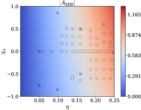
Figure 2 displays select QNM amplitudes, phases, as well as model validation. The left panel of Fig. 2 compares calibration points (colored circles) with the model for $|A_{2220}|$ over the $(\eta,\chi_{s})$ parameter space. Color differences between calibration points and the model’s smooth gradient correspond to noise within the calibration set.

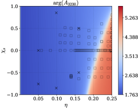
As in Ref. London et al. (2014), $A_{3230}$ and $A_{4440}$ are found to have nonmonotonic amplitudes which correspond to rapid and localized changes in relative phase, $\arg(A_{\bar{\ell}\bar{m}\ell n})$. Due to nonprecessing symmetry, these are the strongest subdominant QNMs for equal-mass BBHs Blanchet (2014); Cotesta et al. (2018). In the central panel of Fig 2, we see for the first time that these abrupt transitions in phase are a robust feature of the nonprecessing parameter space.

VI Model Validation

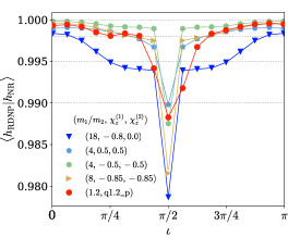
The right panel of Fig. 2 shows validation of RDNP against 5 select non-calibration NR waveforms from the BAM code Brügmann et al. (2008b); Husa et al. (2008).

Figure 3: Posterior sample postprocessing for GW150914: All panels show normalized posterior distributions, with related medians and $90\%$ credible intervals in legends. Median values are shown with dotted lines. Left: Signal to noise ratio (SNR) attributed to each QNM with indices $(\ell,\bar{m},n)$ within a spherical multipole with indices $(\bar{\ell},\bar{m})$ formatted as $(\bar{\ell},\bar{m},\ell,n)$. The attributed SNR for the two most significant QNMs are shown. The optimal SNR, which is the GR prediction for the total ringdown SNR, is shown for reference. Right: GR predictions for absolute QNM amplitudes via Eqs. (8)-(15). Here medians and credible intervals are scaled by $10^{21}$.

Here, NR ringdown plays the role of a hypothetical signal at inclination $\iota$, and RDNP plays the role of a template at the same inclination, with independent polarization and orbital phase. The normalized inner product, or match, $(h_{\mathrm{RDNP}}|h_{\mathrm{NR}})$, is weighted by the anticipated advanced LIGO (Adv. LIGO) zero-detuned noise power spectrum at design sensitivity  Shoemaker et al. (2010) and calculated following Eq. (46) of Ref. Harry et al. (2016), with a starting frequency $f_{\mathrm{min}}=30$ Hz for the integral. RDNP is evaluated at the same intrinsic parameters as the NR waveform such that there are no spin components within the orbital plane. RDNP matches extremely well with NR cases in and out of the calibration region, often having matches above 0.998. This is the case even for a precessing waveform, “q1.2_p”, similar to GW150914 Abbott et al. (2016c). Not shown is the high spin aligned validation case $(M_{1}/M_{2}=8,\chi_{s}=0.85)$. The nonlinear regime for this system extends to approximately $40\leavevmode\nobreak\ M$. When taking this into account, RDNP matches as low as 0.97 for $\iota\approx\pi/2$, but 0.99 and well above for $|\iota-\pi/2|>\pi/6$.

VII Discussion

RDNP has been presented to model the ringdown of nonprecessing BBH systems. While RDNP matches well with NR simulations, there are multiple avenues for improvement. RDNP does not model precession. RDNP also does not model the apparent nonlinear QNMs reported in Ref. London et al. (2014). This may be most important for systems with high aligned spins, where the nonlinear regime is extended.

RDNP provides redundant mode information. For example, via Equation (4), $A_{32320}$ and $A_{32220}$ differ only by factors of $\sigma_{\bar{\ell}\bar{m}\ell\bar{m}n}$. This allows RDNP’s consistency with perturbation theory to be quantified by comparing modeled ratios of $\sigma_{\bar{\ell}\bar{m}\ell\bar{m}n}$ to perturbation theory predictions Kelly and Baker (2013); London et al. (2014). For RDNP, ratios of $\sigma_{\bar{\ell}\bar{m}\ell\bar{m}n}$ agree with perturbation theory within $5\%$ in amplitude and $15\%$ in phase. This agreement could be improved in future treatments.

Future ringdown models should be calibrated to a larger set of more accurate NR simulations. Like Ref. Baibhav et al. (2018), the current work is limited by quality concerns between simulations of different numerical codes. RDNP and related techniques may of be of use in constructing NR-tuned full signal models with accurate mergers. In particular, RDNP may be interfaced directly with the analytic merger-ringdown ansatz proposed in Ref. McWilliams (2019). Primarily, it is expected that RDNP may be of use aiding tests of GR during LIGO’s third observing run. In that setting, many practical questions regarding ringdown are pertinent.

VII.1 Data analysis example

The following questions are briefly considered: How much SNR is in ringdown? How much SNR can be attributed to subdominant QNMs? Can the QNM amplitudes be constrained, and can their relative phases? To proceed, RDNP is applied to inferred posteriors of GW150914’s parameters via a higher-multipole inspiral-merger-ringdown model, PhenomHM London et al. (2018). Here, PhenomHM is applied to the Bayesian inference of GW150914 Vallisneri et al. (2015), according to Ref. Abbott et al. (2016c), and then posterior samples are input to RDNP to yield GR predictions for quantities reported in Figure 3. This approach yields GR predictions independently of individual mode signal-to-noise ratio (SNR) Berti et al. (2006).

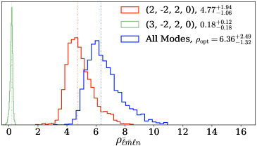
The top panel of Fig. 3 shows the posterior distribution for $\rho_{\mathrm{opt}}$, the estimated total ringdown SNR (red) for GW150914 Usman et al. (2016); Finn (2001). Note that the approximately face-off nature of GW150914 means that $m<0$ QNMs are prevalent Abbott et al. (2016c). Additional posteriors are shown for the SNR contributed by a single QNM

$$\rho_{\bar{\ell}\bar{m}\ell n}=\rho_{\mathrm{opt}}-\rho_{\mathrm{opt|\bar{\ell}\bar{m}\ell n}}\;,$$

where the single interferometer $\rho_{\mathrm{opt|\bar{\ell}\bar{m}\ell n}}^{2}$ is the inner product between a RDNP evaluation with all QNMs, and without the $(\bar{\ell},\bar{m},\ell,n)$ mode. Not surprisingly, the majority of the ringdown SNR can be attributed to the dominant quadrupole, $A_{2-220}$.

Intriguingly, Figure 3’s suggests that the total amount of SNR attributed to subdominant modes is of order 1. It is found that the distribution of SNR attributed to the subdominant modes indeed yields

$$\rho_{\mathrm{opt}}-\rho_{2-220}=1.63^{+0.86}_{-0.72}\;.$$

This order 1 contributed SNR is explained by $\rho_{\mathrm{opt}}^{2}$ having cross terms that are proportional to $\rho_{2-220}\,\rho_{\bar{\ell}\bar{m}\ell n}$, meaning that the larger $\rho_{2-220}$, the larger the effect of $\rho_{\bar{\ell}\bar{m}\ell n}$ on $\rho_{\mathrm{opt}}$.

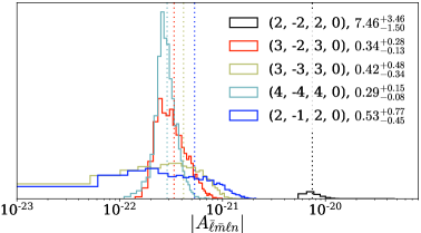
The right panel of Fig. 3 shows GR predictions for QNM amplitudes. For the first time it can be seen that QNMs with odd $m$ have amplitudes which are difficult to constrain. Equations (8)-(15), along with well known difficulty measuring component spins (e.g. Pürrer et al. (2016)), yield a straightforward explanation: uncertainty in $A_{\bar{\ell}\bar{m}\ell n}$ with odd $m$ is dominated by uncertainty in the component spins. Detector networks with greater sensitivity and more interferometers may overcome this limitation Pürrer et al. (2016).

The amount of SNR attributed to higher QNMs and the possibility of using the QNM amplitudes and the relative phase of Eqs. (8)-(15) to test GR illuminates a need to further development of analysis pipelines. Much work has been done in this regard (e.g. Gossan et al. (2012); Bhagwat et al. (2016)), and the interface of RDNP with existing pipelines is ongoing  LAL .

VII.2 Informing analytic ringdown

While this work develops a numerical representation for ringdown, an analytic theory linking ringdown excitations to the initial binary is at present nonexistent.

It may be postulated that such a theory requires physical choices about an observer’s time coordinate relative to features in the full gravitational wave signal. The work presented here strongly suggests that the natural reference time for ringdown is near the peak strain. This result is observationally convenient, given the amount of signal power in that regime. However, it is also counterintuitive, as the peak strain resides in a nonperturbative regime, where the remnant BH is not Kerr Bhagwat et al. (2016).

It is also apparent in this work that any potential analytic theory of ringdown excitation must reproduce the abrupt transitions in phase seen in Figure 2. These transitions have no counterpart in the treatment of inspiral, despite the fact that, the lowest order scaling of PN and QNM amplitudes appears to be identical London et al. (2014).

In total, the results presented here may not only aid tests of GR, but they may also help motivate and constrain an analytic (PN-like) theory of ringdown, one in which ringdown amplitudes are linked to the nonperturbative regime, yet manifestly consistent with linear BH perturbation theory.

$$A_{2220}\; =\;\eta\,(\,-0.6537\,\chi_{s}\;+\;-4.0071\;)$$ (8)

$$A_{2120}\; =\;\eta\,(\,2.3488\,e^{2.6631i}\,\delta\;+\;(0.8011\,e^{5.7070i})\,\chi_{a}+\;(3.5828\,e^{5.5223i})\,\eta\,\delta\;+\;(1.1774\,e^{0.4254i})\,\chi_{s}\,\delta$$ (9)

$$\quad\;+\;(0.6260\,e^{5.3457i})\,\chi_{s}\,\chi_{a}\;)$$

$$A_{3330}\; =\;\eta\,(\,2.6412\,e^{2.9880i}\,\delta\;+\;(1.6030\,e^{0.6655i})\,{\delta}^{2}+\;(1.0354\,e^{3.6096i})\,\chi_{s}\,\delta\;+\;(0.4911\,e^{4.7347i})\,{\chi_{a}}^{2}\;)$$ (10)

$$A_{3230}\; =\;\eta\,(\,2.5707\,e^{4.1427i}\,\eta\;+\;(9.4216\,e^{0.8076i})\,{\eta}^{2}+\;(0.5973\,e^{2.1816i})\,\eta\,\chi_{s}\;+\;(0.2104\,e^{4.9043i})\,{\chi_{a}}^{2}$$ (11)

$$\quad\;+\;(0.4417\,e^{5.4544i})\,\chi_{a}\,\delta\;+\;(0.9439\,e^{1.7614i})\,{\delta}^{2}\;)$$

$$A_{3220}\; =\;\eta\,(\,1.3407\,e^{2.9466i}\,\eta\;+\;(0.0717\,e^{5.5304i})+\;(0.1061\,e^{2.6432i})\,{\chi_{s}}^{2}\;+\;(0.9894\,e^{2.9294i})\,\eta\,\chi_{s}+\;(0.3735\,e^{3.3290i})\,\chi_{a}\,\delta\;)$$ (12)

$$A_{4440}\; =\;\eta\,(\,1.3284\,e^{2.6831i}\,{\delta}^{2}\;+\;(1.1619\,e^{0.4142i})\,{\delta}^{3}+\;(1.2790\,e^{4.7226i})\,\chi_{s}\,{\chi_{a}}^{2}\,\delta\;+\;(1.2387\,e^{4.5616i})\,\chi_{s}\,{\chi_{a}}^{3}$$ (13)

$$\quad\;+\;(1.2909\,e^{2.8120i})\,\chi_{s}\,{\delta}^{3}\;+\;(42.3575\,e^{6.1418i})\,{\eta}^{4}\;)$$

$$A_{4330}\; =\;\eta\,(\,0.0411\,e^{2.6441i}\,\chi_{a}\;+\;(0.0486\,e^{3.2085i})\,{\chi_{s}}^{2}+\;(0.8078\,e^{2.7461i})\,\eta\,\delta\;+\;(0.1940\,e^{3.0292i})\,\chi_{s}\,\delta$$ (14)

$$\quad\;+\;(0.0529\,e^{3.5830i})\,{\chi_{a}}^{2}\;+\;(0.0358\,e^{0.1731i})\,{\delta}^{2}\;)$$

$$A_{4340}\; =\;\eta\,(\,0.5665\,e^{3.3992i}\,\delta\;+\;(0.1457\,e^{4.7476i})\,\chi_{a}+\;(0.8239\,e^{1.8174i})\,\eta\,\chi_{a}\;+\;(0.0507\,e^{4.7495i})\,\chi_{s}\,\chi_{a}$$ (15)

$$\quad\;+\;(0.9806\,e^{0.6029i})\,{\delta}^{3}\;+\;(10.1678\,e^{6.2185i})\,{\eta}^{2}\,\delta\;)$$

VIII Acknowledgements

The author thanks Mark Hannam, Sascha Husa and Scott Hughes for useful discussions and access to their numerical waveforms. Additional thanks are extended to the LIGO-Virgo collaboration for their comments and review. This research has made use of data, software and/or web tools obtained from the LIGO Open Science Center, a service of LIGO Laboratory, the LIGO Scientific Collaboration and the Virgo Collaboration. LIGO is funded by the U.S. National Science Foundation. Virgo is funded by the French Centre National de Recherche Scientifique (CNRS), the Italian Istituto Nazionale della Fisica Nucleare (INFN) and the Dutch Nikhef, with contributions by Polish and Hungarian institutes. The work presented in this paper was supported by Science and Technology Facilities Council (STFC) Grant No. ST/L000962/1, European Research Council Consolidator Grant No. 647839, Spanish Ministry of Economy and Competitiveness Grants No. CSD2009-00064, No. FPA2013-41042-P and No. FPA2016-76821-P, the Spanish Agencia Estatal de Investigación, European Union FEDER funds, Vicepresidència i Conselleria d’Innovació, Recerca i Turisme, Conselleria d’Educació, i Universitats del Govern de les Illes Balears, and the Fons Social Europeu. BAM simulations were carried out at Advanced Research Computing (ARCCA) at Cardiff, as part of the European PRACE petascale computing initiative on the clusters Hermit, Curie and SuperMUC, on the U.K. DiRAC Datacentric cluster and on the BSC MareNostrum computer under PRACE and RES (Red Española de Supercomputación) allocations.

References

- Abbott et al. (2017a) B. P. Abbott et al. (Virgo and LIGO Scientific), Phys. Rev. Lett. 119, 141101 (2017a).
- Abbott et al. (2017b) B. P. Abbott et al. (VIRGO and LIGO Scientific), Phys. Rev. Lett. 118, 221101 (2017b).
- Abbott et al. (2016a) B. P. Abbott et al. (Virgo and LIGO Scientific), Phys. Rev. Lett. 116, 221101 (2016a).
- Yunes et al. (2016) N. Yunes, K. Yagi, and F. Pretorius, Phys. Rev. D 94, 084002 (2016).
- Abbott et al. (2016b) B. P. Abbott et al. (Virgo and LIGO Scientific), Phys. Rev. X 6, 041015 (2016b).
- Unnikrishnan (2013) C. S. Unnikrishnan, Int. J. Mod. Phys. D 22, 1341010 (2013).
- Kanda et al. (2017) N. Kanda et al. (KAGRA), in 14th Marcel Grossmann Meeting on Recent Developments in Theoretical and Experimental General Relativity, Astrophysics, and Relativistic Field Theories, Vol. 3 (2017) pp. 3159–3163.
- Maselli et al. (2017) A. Maselli, K. Kokkotas, and P. Laguna, Phys. Rev. D 95, 104026 (2017), arXiv:1702.01110 [gr-qc] .
- Tang et al. (2018) Y. Tang, Z. Haiman, and A. Macfadyen, Mon. Not. R. Astron. Soc. 476, 2249 (2018).
- Bhagwat et al. (2016) S. Bhagwat, D. A. Brown, and S. W. Ballmer, Phys. Rev. D 94, 084024 (2016).
- Baibhav et al. (2018) V. Baibhav, E. Berti, V. Cardoso, and G. Khanna, Phys. Rev. D 97, 044048 (2018).
- Berti et al. (2016) E. Berti, A. Sesana, E. Barausse, V. Cardoso, and K. Belczynski, Phys. Rev. Lett. 117, 101102 (2016).
- Yang et al. (2017) H. Yang, K. Yagi, J. Blackman, L. Lehner, V. Paschalidis, F. Pretorius, and N. Yunes, Phys. Rev. Lett. 118, 161101 (2017).
- Cabero et al. (2018) M. Cabero, C. D. Capano, O. Fischer-Birnholtz, B. Krishnan, A. B. Nielsen, A. H. Nitz, and C. M. Biwer, Phys. Rev. D 97, 124069 (2018).
- Leaver and Chandrasekhar (1985) E. W. Leaver and S. Chandrasekhar, Proc. R. Soc. A 402, 285 (1985).
- Teukolsky (1972) S. A. Teukolsky, Phys. Rev. Lett. 29, 1114 (1972).
- Nollert and Price (1999) H.-P. Nollert and R. H. Price, J. Math. Phys. (N.Y.) 40, 980 (1999).
- Kokkotas and Schmidt (1999) K. D. Kokkotas and B. G. Schmidt, Living Rev. Relativity 2 (1999).
- Berti et al. (2009) E. Berti, V. Cardoso, and A. O. Starinets, Classical Quantum Gravity 26, 163001 (2009).
- Gürlebeck (2015) N. Gürlebeck, Phys. Rev. Lett. 114, 151102 (2015).
- Gossan et al. (2012) S. Gossan, J. Veitch, and B. Sathyaprakash, Phys.Rev. D 85, 124056 (2012).
- Meidam et al. (2014) J. Meidam, M. Agathos, C. Van Den Broeck, J. Veitch, and B. S. Sathyaprakash, Phys. Rev. D 90, 064009 (2014).
- Berti et al. (2006) E. Berti, V. Cardoso, and C. M. Will, Phys. Rev. D 73, 064030 (2006).
- Kamaretsos et al. (2012a) I. Kamaretsos, M. Hannam, S. Husa, and B. Sathyaprakash, Phys.Rev. D 85, 024018 (2012a).
- Buonanno et al. (2007) A. Buonanno, G. B. Cook, and F. Pretorius, Phys.Rev. D 75, 124018 (2007).
- Berti et al. (2007) E. Berti, V. Cardoso, J. A. Gonzalez, U. Sperhake, M. Hannam, S. Husa, and B. Brügmann, Phys. Rev. D 76, 064034 (2007).
- London et al. (2014) L. London, D. Shoemaker, and J. Healy, Phys. Rev. D 90, 124032 (2014).
- McWilliams (2019) S. T. McWilliams, Phys. Rev. Lett. 122, 191102 (2019).
- London et al. (2018) L. London, S. Khan, E. Fauchon-Jones, C. García, M. Hannam, S. Husa, X. Jiménez-Forteza, C. Kalaghatgi, F. Ohme, and F. Pannarale, Phys. Rev. Lett. 120, 161102 (2018).
- Cotesta et al. (2018) R. Cotesta, A. Buonanno, A. Bohé, A. Taracchini, I. Hinder, and S. Ossokine, Phys. Rev. D 98, 084028 (2018).
- Varma et al. (2019) V. Varma, S. E. Field, M. A. Scheel, J. Blackman, L. E. Kidder, and H. P. Pfeiffer, Phys. Rev. D 99, 064045 (2019), arXiv:1812.07865 [gr-qc] .
- Carullo et al. (2018) G. Carullo et al., Phys. Rev. D 98, 104020 (2018), arXiv:1805.04760 [gr-qc] .
- Carullo et al. (2019) G. Carullo, W. Del Pozzo, and J. Veitch, Phys. Rev. D 99, 123029 (2019), [Erratum: Phys.Rev.D 100, 089903 (2019)], arXiv:1902.07527 [gr-qc] .
- Jani et al. (2016) K. Jani, J. Healy, J. A. Clark, L. London, P. Laguna, and D. Shoemaker, Classical Quantum Gravity 33, 204001 (2016).
- Brügmann et al. (2008a) B. Brügmann, J. A. Gonzalez, M. Hannam, S. Husa, U. Sperhake, and W. Tichy, Phys. Rev. D 77, 024027 (2008a).
- Husa et al. (2008) S. Husa, J. A. González, M. Hannam, B. Brügmann, and U. Sperhake, Classical Quantum Gravity 25, 105006 (2008).
- Ruiz et al. (2008) M. Ruiz, M. Alcubierre, D. Núñez, and R. Takahashi, General Relativ. and Gravit. 40, 1705 (2008).
- Kelly and Baker (2013) B. J. Kelly and J. G. Baker, Phys.Rev. D 87, 084004 (2013).
- Press and Teukolsky (1973) W. H. Press and S. A. Teukolsky, Astrophys. J. 185, 649 (1973).
- Berti and Klein (2014) E. Berti and A. Klein, Phys. Rev. D 90, 064012 (2014).
- London and Fauchon-Jones (2019) L. London and E. Fauchon-Jones, Classical Quantum Gravity 36, 235015 (2019), arXiv:1810.03550 [gr-qc] .
- Kamaretsos et al. (2012b) I. Kamaretsos, M. Hannam, and B. Sathyaprakash, Phys.Rev.Lett. 109, 141102 (2012b).
- Husa et al. (2016) S. Husa, S. Khan, M. Hannam, M. Pürrer, F. Ohme, X. Jiménez Forteza, and A. Bohé, Phys. Rev. D 93, 044006 (2016).
- Frauendiener (2011) J. Frauendiener, Gen. Relativ. Gravit. 43, 2931 (2011).
- Healy and Lousto (2017) J. Healy and C. O. Lousto, Phys. Rev. D 95, 024037 (2017).
- Jiménez-Forteza et al. (2017) X. Jiménez-Forteza, D. Keitel, S. Husa, M. Hannam, S. Khan, and M. Pürrer, Phys. Rev. D 95, 064024 (2017).
- Blanchet (2014) L. Blanchet, Living Rev. Rel. 17, 2 (2014).
- Brügmann et al. (2008b) B. Brügmann, J. A. González, M. Hannam, S. Husa, U. Sperhake, and W. Tichy, Phys. Rev. D 77, 024027 (2008b).
- Shoemaker et al. (2010) D. Shoemaker et al. (LIGO Scientific Collaboration), LIGO-T0900288, https://dcc.ligo.org/ (2010).
- Harry et al. (2016) I. Harry, S. Privitera, A. Bohé, and A. Buonanno, Phys. Rev. D 94, 024012 (2016).
- Abbott et al. (2016c) B. P. Abbott et al. (Virgo and LIGO Scientific Collaboration), Phys. Rev. Lett. 116, 241102 (2016c).
- Vallisneri et al. (2015) M. Vallisneri, J. Kanner, R. Williams, A. Weinstein, and B. Stephens, J. Phys. Conf. Ser. 610, 012021 (2015).
- Usman et al. (2016) S. A. Usman et al., Classical Quantum Gravity 33, 215004 (2016).
- Finn (2001) L. S. Finn, Phys. Rev. D 63, 102001 (2001).
- Pürrer et al. (2016) M. Pürrer, M. Hannam, and F. Ohme, Phys. Rev. D 93, 084042 (2016).
- (56) “https://losc.ligo.org/,” .