Incremental Eigenpair Computation for Graph Laplacian Matrices: Theory and Applications

Abstract

The smallest eigenvalues and the associated eigenvectors (i.e., eigenpairs) of a graph Laplacian matrix have been widely used in spectral clustering and community detection. However, in real-life applications the number of clusters or communities (say, $K$) is generally unknown a-priori. Consequently, the majority of the existing methods either choose $K$ heuristically or they repeat the clustering method with different choices of $K$ and accept the best clustering result. The first option, more often, yields suboptimal result, while the second option is computationally expensive. In this work, we propose an incremental method for constructing the eigenspectrum of the graph Laplacian matrix. This method leverages the eigenstructure of graph Laplacian matrix to obtain the $K$-th smallest eigenpair of the Laplacian matrix given a collection of all previously computed $K-1$ smallest eigenpairs. Our proposed method adapts the Laplacian matrix such that the batch eigenvalue decomposition problem transforms into an efficient sequential leading eigenpair computation problem. As a practical application, we consider user-guided spectral clustering. Specifically, we demonstrate that users can utilize the proposed incremental method for effective eigenpair computation and for determining the desired number of clusters based on multiple clustering metrics.

1 Introduction

Over the past two decades, the graph Laplacian matrix and its variants have been widely adopted for solving various research tasks, including graph partitioning pothen1990partitioning , data clustering Luxburg07 ; wu2016revisiting ; chen2016efficient , community detection White05 ; CPY14spectral ; chen2017revisiting , consensus in networks Olfati-Saber07 ; wu2009empirical , accelerated distributed optimization liu2017accelerated , dimensionality reduction belkin2003laplacian ; wu2016estimating , entity disambiguation ZhangSaha14 ; Zhang.Dundar.ea:16 ; Zhang.Hasan.3 ; tkde_online ; Zhang.Noman.ea:17 ; Zhang.Hasan.ea:15 , link prediction Hasan06linkprediction ; Hasan2011 ; Zhang.Hasan.ea:16 ; icde-sutanay , graph signal processing Shuman13 ; chen2017bias , centrality measures for graph connectivity CPY14deep , multi-layer network analysis chen_tsipn ; weiyi , interconnected physical systems Radicchi13 , network vulnerability assessment CPY14ComMag , image segmentation Shi00 ; icmla-dundar , gene expression zifan1 ; zifan2 ; liu2017genome , among others. The fundamental task is to represent the data of interest as a graph for analysis, where a node represents an entity (e.g., a pixel in an image or a user in an online social network) and an edge represents similarity between two multivariate data samples or actual relation (e.g., friendship) between nodes Luxburg07 . More often the $K$ eigenvectors associated with the $K$ smallest eigenvalues of the graph Laplacian matrix are used to cluster the entities into $K$ clusters of high similarity. For brevity, throughout this paper we will call these eigenvectors as the $K$ smallest eigenvectors.

The success of graph Laplacian matrix based methods for graph partitioning and spectral clustering can be explained by the fact that acquiring $K$ smallest eigenvectors is equivalent to solving a relaxed graph cut minimization problem, which partitions a graph into $K$ clusters by minimizing various objective functions including min cut, ratio cut or normalized cut Luxburg07 . Generally, in clustering the value $K$ is selected to be much smaller than $n$ (the number of data points), making full eigen decomposition (such as QR decomposition) unnecessary. An efficient alternative is to use methods that are based on power iteration, such as Arnoldi method or Lanczos method, which computes the leading eigenpairs through repeated matrix vector multiplication wu2015preconditioned ; wu2017primme_svds . ARPACK lehoucq1998arpack library is a popular parallel implementation of different variants of Arnoldi and Lanczos methods, which is used by many commercial software including Matlab.

However, in most situations the best value of $K$ is unknown and a heuristic is used by clustering algorithms to determine the number of clusters, e.g., fixing a maximum number of clusters $K_{\max}$ and detecting a large gap in the values of the $K_{\max}$ largest sorted eigenvalues or normalized cut score Polito01grouping ; ng2002spectral . Alternatively, this value of $K$ can be determined based on domain knowledge basu2004active . For example, a user may require that the largest cluster size be no more than 10% of the total number of nodes or that the total inter-cluster edge weight be no greater than a certain amount. In these cases, the desired choice of $K$ cannot be determined a priori. Over-estimation of the upper bound $K_{\max}$ on the number of clusters is expensive as the cost of finding $K$ eigenpairs using the power iteration method grows rapidly with $K$. On the other hand, choosing an insufficiently large value for $K_{\max}$ runs the risk of severe bias. Setting $K_{\max}$ to the number of data points $n$ is generally computationally infeasible, even for a moderate-sized graph. Therefore, an incremental eigenpair computation method that effectively computes the $K$-th smallest eigenpair of graph Laplacian matrix by utilizing the previously computed $K-1$ smallest eigenpairs is needed. Such an iterative method obviates the need to set an upper bound $K_{\max}$ on $K$, and its efficiency can be explained by the adaptivity to increments in $K$.

By exploiting the special matrix properties and graph characteristics of a graph Laplacian matrix, we propose an efficient method for computing the $(K+1)$-th eigenpair given all of the $K$ smallest eigenpairs, which we call the Incremental method of Increasing Orders (Incremental-IO). For each increment, given the previously computed smallest eigenpairs, we show that computing the next smallest eigenpair is equivalent to computing a leading eigenpair of a particular matrix, which transforms potentially tedious numerical computation (such as the iterative tridiagonalization and eigen-decomposition steps in the Lanczos algorithm lanczos1950iteration ) to simple matrix power iterations of known computational efficiency kuczynski1992estimating . Specifically, we show that Incremental-IO can be implemented via power iterations, and analyze its computational complexity and data storage requirements. We then compare the performance of Incremental-IO with a batch computation method which computes all of the $K$ smallest eigenpairs in a single batch, and an incremental method adapted from the Lanczos algorithm, which we call the Lanczos method of Increasing Orders (Lanczos-IO). For a given number of eigenpairs $K$ iterative matrix-vector multiplication of Lanczos procedure yields a set of Lanczos vectors ($\mathbf{Q}_{\ell}$), and a tridiagonal matrix ($\mathbf{T}_{\ell}$), followed by a full eigen-decomposition of $\mathbf{T}_{\ell}$ ($\ell$ is a value much smaller than the matrix size). Lanczos-IO saves the Lanczos vectors that were obtained while $K$ eigenpairs were computed and used those to generate new Lanczos vectors for computing the $(K+1)$-th eigenpair.

Comparing to the batch method, our experimental results show that for a given order $K$, Incremental-IO provides a significant reduction in computation time. Also, as $K$ increases, the gap between Incremental-IO and the batch approach widens, providing an order of magnitude speed-up. Experiments on real-life datasets show that the performance of Lanczos-IO is overly sensitive to the selection of augmented Lanczos vectors, a parameter that cannot be optimized a priori—for some of our experimental datasets, Lanczos-IO performs even worse than the batch method (see Sec. 6). Moreover, Lanczos-IO consumes significant amount of memory as it has to save the Lanczos vectors ($\mathbf{Q}_{\ell}$) for making the incremental approach realizable. In summary, Lanczos-IO, although an incremental eigenpair computation algorithm, falls short in terms of robustness.

To illustrate the real-life utility of incremental eigenpair computation methods, we design a user-guided spectral clustering algorithm which uses Incremental-IO. The algorithm provides clustering solution for a sequence of $K$ values efficiently, and thus enable a user to compare these clustering solutions for facilitating the selection of the most appropriate clustering.

The contributions of this paper are summarized as follows:

1. We propose an incremental eigenpair computation method (Incremental-IO) for both unnormalized and normalized graph Laplacian matrices, by transforming the original eigenvalue decomposition problem into an efficient sequential leading eigenpair computation problem. Specifically, Incremental-IO can be implemented via power iterations, which possess efficient computational complexity and data storage. Simulation results show that Incremental-IO generates the desired eigenpair accurately and has superior performance over the batch computation method in terms of computation time.

2. We show that Incremental-IO is robust in comparison to Lanczos-IO, which is an incremental eigenpair method that we design by adapting the Lanczos method.

3. We use several real-life datasets to demonstrate the utility of Incremental-IO. Specifically, we show that Incremental-IO is suitable for user-guided spectral clustering which provides a sequence of clustering results for unit increment of the number $K$ of clusters, and updates the associated cluster evaluation metrics for helping a user in decision making.

2 Related Work

2.1 Incremental eigenvalue decomposition

The proposed method (Incremental-IO) aims to incrementally compute the smallest eigenpair of a given graph Laplacian matrix. There are several works that are named as incremental eigenvalue decomposition methods ning2007incremental ; jia2009incremental ; ning2010incremental ; dhanjal2014efficient ; ranjan2014incremental . However, these works focus on updating the eigenstructure of graph Laplacian matrix of dynamic graphs when nodes (data samples) or edges are inserted or deleted from the graph, which are fundamentally different from incremental computation of eigenpairs of increasing orders. Consequently, albeit similarity in research topics, they are two distinct sets of problems and cannot be directly compared.

2.2 Cluster Count Selection for Spectral Clustering

Many spectral clustering algorithms utilize the eigenstructure of graph Laplacian matrix for selecting number of clusters. In Polito01grouping , a value $K$ that maximizes the gap between the $K$-th and the $(K+1)$-th smallest eigenvalue is selected as the number of clusters. In ng2002spectral , a value $K$ that minimizes the sum of cluster-wise Euclidean distance between each data point and the centroid obtained from K-means clustering on $K$ smallest eigenvectors is selected as the number of clusters. In zelnik2004self , the smallest eigenvectors of normalized graph Laplacian matrix are rotated to find the best alignment that reflects the true clusters. A model based method for determining the number of clusters is proposed in Poon2012 . In chen2016phase , a model order selection criterion for identifying the number of clusters is proposed by estimating the interconnectivity of the graph using the eigenpairs of the graph Laplacian matrix. In van2001graph , the clusters are identified via random walk on graphs. In blondel2008fast , an iterative greedy modularity maximization approach is proposed for clustering. In Krzakala2013 ; Saade2015spectral , the eigenpairs of the nonbacktracking matrix are used to identify clusters. Note that aforementioned methods use only one single clustering metric to determine the number of clusters and often implicitly assume an upper bound on $K$ (namely $K_{\max}$). As demonstrated in Sec. 6, the proposed incremental eigenpair computation method (Incremental-IO) can be used to efficiently provide a sequence of clustering results for unit increment of the number $K$ of clusters and updates the associated (potentially multiple) cluster evaluation metrics.

3 Incremental Eigenpair Computation for Graph Laplacian Matrices

3.1 Background

Throughout this paper bold uppercase letters (e.g., $\mathbf{X}$) denote matrices and $\mathbf{X}_{ij}$ (or $[\mathbf{X}]_{ij}$) denotes the entry in $i$-th row and $j$-th column of $\mathbf{X}$, bold lowercase letters (e.g., $\mathbf{x}$ or $\mathbf{x}_{i}$) denote column vectors, $(\cdot)^{T}$ denotes matrix or vector transpose, italic letters (e.g., $x$ or $x_{i}$) denote scalars, and calligraphic uppercase letters (e.g., $\mathcal{X}$ or $\mathcal{X}_{i}$) denote sets. The $n\times 1$ vector of ones (zeros) is denoted by $\mathbf{1}_{n}$ ($\mathbf{0}_{n}$). The matrix $\mathbf{I}$ denotes an identity matrix and the matrix $\mathbf{O}$ denotes the matrix of zeros.

We use two $n\times n$ symmetric matrices, $\mathbf{A}$ and $\mathbf{W}$, to denote the adjacency and weight matrices of an undirected weighted simple graph $G$ with $n$ nodes and $m$ edges. $\mathbf{A}_{ij}=1$ if there is an edge between nodes $i$ and $j$, and $\mathbf{A}_{ij}=0$ otherwise. $\mathbf{W}$ is a nonnegative symmetric matrix such that $\mathbf{W}_{ij}\geq 0$ if $\mathbf{A}_{ij}=1$ and $\mathbf{W}_{ij}=0$ if $\mathbf{A}_{ij}=0$. Let $s_{i}=\sum_{j=1}^{n}\mathbf{W}_{ij}$ denote the strength of node $i$. Note that when $\mathbf{W}=\mathbf{A}$, the strength of a node is equivalent to its degree. $\mathbf{S}=\textnormal{diag}(s_{1},s_{2},\ldots,s_{n})$ is a diagonal matrix with nodal strength on its main diagonal and the off-diagonal entries being zero.

The (unnormalized) graph Laplacian matrix is defined as

$$\mathbf{L}=\mathbf{S}-\mathbf{W}.$$ (1)

One popular variant of the graph Laplacian matrix is the normalized graph Laplacian matrix defined as

$$\mathbf{L}_{\mathcal{N}}=\mathbf{S}^{-\frac{1}{2}}\mathbf{L}\mathbf{S}^{-\frac{1}{2}}=\mathbf{I}-\mathbf{S}^{-\frac{1}{2}}\mathbf{W}\mathbf{S}^{-\frac{1}{2}},$$ (2)

where $\mathbf{S}^{-\frac{1}{2}}=\textnormal{diag}(\frac{1}{\sqrt{s_{1}}},\frac{1}{\sqrt{s_{2}}},\ldots,\frac{1}{\sqrt{s_{n}}})$. The $i$-th smallest eigenvalue and its associated unit-norm eigenvector of $\mathbf{L}$ are denoted by $\lambda_{i}(\mathbf{L})$ and $\mathbf{v}_{i}(\mathbf{L})$, respectively. That is, the eigenpair $(\lambda_{i},\mathbf{v}_{i})$ of $\mathbf{L}$ has the relation $\mathbf{L}\mathbf{v}_{i}=\lambda_{i}\mathbf{v}_{i}$, and $\lambda_{1}(\mathbf{L})\leq\lambda_{2}(\mathbf{L})\leq\ldots\leq\lambda_{n}(\mathbf{L})$. The eigenvectors have unit Euclidean norm and they are orthogonal to each other such that $\mathbf{v}_{i}^{T}\mathbf{v}_{j}=1$ if $i=j$ and $\mathbf{v}_{i}^{T}\mathbf{v}_{j}=0$ if $i\neq j$. The eigenvalues of $\mathbf{L}$ are said to be distinct if $\lambda_{1}(\mathbf{L})<\lambda_{2}(\mathbf{L})<\ldots<\lambda_{n}(\mathbf{L})$. Similar notations are used for $\mathbf{L}_{\mathcal{N}}$.

Table 1: Utility of the established lemmas, corollaries, and theorems.

Graph Type / Graph Laplacian Matrix	Unnormalized	Normalized
Connected Graphs	Lemma 1, Theorem 3.1	Corollary 1, Corollary 3
Disconnected Graphs	Lemma 2, Theorem 3.2	Corollary 2, Corollary 4

3.2 Theoretical foundations of the proposed method (Incremental-IO)

The following lemmas and corollaries provide the cornerstone for establishing the proposed incremental eigenpair computation method (Incremental-IO). The main idea is that we utilize the eigenspace structure of graph Laplacian matrix to inflate specific eigenpairs via a particular perturbation matrix, without affecting other eigenpairs. Incremental-IO can be viewed as a specialized Hotelling’s deflation method parlett1980symmetric designed for graph Laplacian matrices by exploiting their spectral properties and associated graph characteristics. It works for both connected, and disconnected graphs using either normalized or unnormalized graph Laplacian matrix. For illustration purposes, in Table 1 we group the established lemmas, corollaries, and theorems under different graph types and different graph Laplacian matrices.

Lemma 1

Assume that $G$ is a connected graph and $\mathbf{L}$ is the graph Laplacian with $s_{i}$ denoting the sum of the entries in the $i$-th row of the weight matrix $\mathbf{W}$. Let $s=\sum_{i=1}^{n}s_{i}$ and define $\widetilde{\mathbf{L}}=\mathbf{L}+\frac{s}{n}\mathbf{1}_{n}\mathbf{1}_{n}^{T}.$ Then the eigenpairs of $\widetilde{\mathbf{L}}$ satisfy $(\lambda_{i}(\widetilde{\mathbf{L}}),\mathbf{v}_{i}(\widetilde{\mathbf{L}}))=(\lambda_{i+1}(\mathbf{L}),\mathbf{v}_{i+1}(\mathbf{L}))$ for $1\leq i\leq n-1$ and $(\lambda_{n}(\widetilde{\mathbf{L}}),\mathbf{v}_{n}(\widetilde{\mathbf{L}}))=(s,\frac{\mathbf{1}_{n}}{\sqrt{n}})$.

Proof

Since $\mathbf{L}$ is a positive semidefinite (PSD) matrix Chung97SpectralGraph , $\lambda_{i}(\mathbf{L})\geq 0$ for all $i$. Since $G$ is a connected graph, by (1) $\mathbf{L}\mathbf{1}_{n}=(\mathbf{S}-\mathbf{W})\mathbf{1}_{n}=\mathbf{0}_{n}$. Therefore, by the PSD property we have $(\lambda_{1}(\mathbf{L}),\mathbf{v}_{1}(\mathbf{L}))=(0,\frac{\mathbf{1}_{n}}{\sqrt{n}})$. Moreover, since $\mathbf{L}$ is a symmetric real-valued square matrix, from (1) we have

$$\textnormal{trace}(\mathbf{L}) =\sum_{i=1}^{n}\mathbf{L}_{ii}$$

$$=\sum_{i=1}^{n}\lambda_{i}(\mathbf{L})$$

$$=\sum_{i=1}^{n}s_{i}$$

$$=s.$$ (3)

By the PSD property of $\mathbf{L}$, we have $\lambda_{n}(\mathbf{L})<s$ since $\lambda_{2}(\mathbf{L})>0$ for any connected graph. Therefore, by the orthogonality of eigenvectors of $\mathbf{L}$ (i.e., $\mathbf{1}_{n}^{T}\mathbf{v}_{i}(\mathbf{L})=0$ for all $i\geq 2$) the eigenvalue decomposition of $\widetilde{\mathbf{L}}$ can be represented as

$$\widetilde{\mathbf{L}} =\sum_{i=2}^{n}\lambda_{i}(\mathbf{L})\mathbf{v}_{i}(\mathbf{L})\mathbf{v}_{i}^{T}(\mathbf{L})+\frac{s}{n}\mathbf{1}_{n}\mathbf{1}_{n}^{T}$$

$$=\sum_{i=1}^{n}\lambda_{i}(\widetilde{\mathbf{L}})\mathbf{v}_{i}(\widetilde{\mathbf{L}})\mathbf{v}_{i}^{T}(\widetilde{\mathbf{L}}),$$ (4)

where $(\lambda_{n}(\widetilde{\mathbf{L}}),\mathbf{v}_{n}(\widetilde{\mathbf{L}}))=(s,\frac{\mathbf{1}_{n}}{\sqrt{n}})$ and $(\lambda_{i}(\widetilde{\mathbf{L}}),\mathbf{v}_{i}(\widetilde{\mathbf{L}}))=$ $(\lambda_{i+1}(\mathbf{L}),\mathbf{v}_{i+1}(\mathbf{L}))$ for $1\leq i\leq n-1$.

Corollary 1

For a normalized graph Laplacian matrix $\mathbf{L}_{\mathcal{N}}$, assume $G$ is a connected graph and let $\widetilde{\mathbf{L}}_{\mathcal{N}}=\mathbf{L}_{\mathcal{N}}+\frac{2}{s}\mathbf{S}^{\frac{1}{2}}\mathbf{1}_{n}\mathbf{1}_{n}^{T}\mathbf{S}^{\frac{1}{2}}$. Then $(\lambda_{i}(\widetilde{\mathbf{L}}_{\mathcal{N}}),\mathbf{v}_{i}(\widetilde{\mathbf{L}}_{\mathcal{N}}))=(\lambda_{i+1}(\mathbf{L}_{\mathcal{N}}),\mathbf{v}_{i+1}(\mathbf{L}_{\mathcal{N}}))$ for $1\leq i\leq n-1$ and $(\lambda_{n}(\widetilde{\mathbf{L}}_{\mathcal{N}}),\mathbf{v}_{n}(\widetilde{\mathbf{L}}_{\mathcal{N}}))=(2,\frac{\mathbf{S}^{\frac{1}{2}}\mathbf{1}_{n}}{\sqrt{s}})$.

Proof

Recall from (2) that $\mathbf{L}_{\mathcal{N}}=\mathbf{S}^{-\frac{1}{2}}\mathbf{L}\mathbf{S}^{-\frac{1}{2}}$, and also we have $\mathbf{L}_{\mathcal{N}}\mathbf{S}^{\frac{1}{2}}\mathbf{1}_{n}=\mathbf{S}^{-\frac{1}{2}}\mathbf{L}\mathbf{1}_{n}=\mathbf{0}_{n}$. Moreover, it can be shown that $0\leq\lambda_{1}(\mathbf{L}_{\mathcal{N}})\leq\lambda_{2}(\mathbf{L}_{\mathcal{N}})\leq\ldots\leq\lambda_{n}(\mathbf{L}_{\mathcal{N}})\leq 2$ Merris94 , and $\lambda_{2}(\mathbf{L}_{\mathcal{N}})>0$ if $G$ is connected. Following the same derivation procedure for Lemma 1 we obtain the corollary. Note that $\mathbf{S}^{\frac{1}{2}}=\textnormal{diag}(\sqrt{s_{1}},\sqrt{s_{2}},\ldots,\sqrt{s_{n}})$ and $(\mathbf{S}^{\frac{1}{2}}\mathbf{1}_{n})^{T}\mathbf{S}^{\frac{1}{2}}\mathbf{1}_{n}=\mathbf{1}_{n}^{T}\mathbf{S}\mathbf{1}_{n}=s$.

Lemma 2

Assume that $G$ is a disconnected graph with $\delta\geq 2$ connected components. Let $s=\sum_{i=1}^{n}s_{i}$, let $\mathbf{V}=[\mathbf{v}_{1}(\mathbf{L}),\mathbf{v}_{2}(\mathbf{L}),\ldots,\mathbf{v}_{\delta}(\mathbf{L})]$, and let $\widetilde{\mathbf{L}}=\mathbf{L}+s\mathbf{V}\mathbf{V}^{T}$. Then $(\lambda_{i}(\widetilde{\mathbf{L}}),\mathbf{v}_{i}(\widetilde{\mathbf{L}}))=(\lambda_{i+\delta}(\mathbf{L}),\mathbf{v}_{i+\delta}(\mathbf{L}))$ for $1\leq i\leq n-\delta$, $\lambda_{i}(\widetilde{\mathbf{L}})=s$ for $n-\delta+1\leq i\leq n$, and $[\mathbf{v}_{n-\delta+1}(\widetilde{\mathbf{L}}),\mathbf{v}_{n-\delta+2},(\widetilde{\mathbf{L}}),\ldots,\mathbf{v}_{n}(\widetilde{\mathbf{L}})]=\mathbf{V}$.

Proof

The graph Laplacian matrix of a disconnected graph consisting of $\delta$ connected components can be represented as a matrix with diagonal block structure, where each block in the diagonal corresponds to one connected component in $G$CPY13GlobalSIP , that is,

$$\mathbf{L}=\left[\begin{matrix}\mathbf{L}_{1}&\mathbf{O}&\mathbf{O}&\mathbf{O}\\ \mathbf{O}&\mathbf{L}_{2}&\mathbf{O}&\mathbf{O}\\ \mathbf{O}&\mathbf{O}&\ddots&\mathbf{O}\\ \mathbf{O}&\mathbf{O}&\mathbf{O}&\mathbf{L}_{\delta}\end{matrix}\right],$$ (5)

where $\mathbf{L}_{k}$ is the graph Laplacian matrix of $k$-th connected component in $G$. From the proof of Lemma 1 each connected component contributes to exactly one zero eigenvalue for $\mathbf{L}$, and

$$\lambda_{n}(\mathbf{L}) <\sum_{k=1}^{\delta}\sum_{i\in\text{component}~{}k}\lambda_{i}(\mathbf{L}_{k})$$

$$=\sum_{k=1}^{\delta}\sum_{i\in\text{component}~{}k}s_{i}$$

$$=s.$$ (6)

Therefore, we have the results in Lemma 2.

Lemma 1 applies to the (unnormalized) graph Laplacian matrix of a connected graph, and the corollary below applies to the normalized graph Laplacian matrix of a connected graph.

Corollary 2

For a normalized graph Laplacian matrix $\mathbf{L}_{\mathcal{N}}$, assume $G$ is a disconnected graph with $\delta\geq 2$ connected components. Let $\mathbf{V}_{\delta}=[\mathbf{v}_{1}(\mathbf{L}_{\mathcal{N}}),\mathbf{v}_{2}(\mathbf{L}_{\mathcal{N}}),\\ \ldots,\mathbf{v}_{\delta}(\mathbf{L}_{\mathcal{N}})]$, and let $\widetilde{\mathbf{L}}_{\mathcal{N}}=\mathbf{L}_{\mathcal{N}}+2\mathbf{V}_{\delta}\mathbf{V}_{\delta}^{T}.$ Then $(\lambda_{i}(\widetilde{\mathbf{L}}_{\mathcal{N}}),\mathbf{v}_{i}(\widetilde{\mathbf{L}}_{\mathcal{N}}))=(\lambda_{i+\delta}(\mathbf{L}_{\mathcal{N}}),\\ \mathbf{v}_{i+\delta}(\mathbf{L}_{\mathcal{N}}))$ for $1\leq i\leq n-\delta$, $\lambda_{i}(\widetilde{\mathbf{L}}_{\mathcal{N}})=2$ for $n-\delta+1\leq i\leq n$, and $[\mathbf{v}_{n-\delta+1}(\widetilde{\mathbf{L}}_{\mathcal{N}}),\mathbf{v}_{n-\delta+2},(\widetilde{\mathbf{L}}_{\mathcal{N}}),\ldots,\mathbf{v}_{n}(\widetilde{\mathbf{L}}_{\mathcal{N}})]=\mathbf{V}_{\delta}$.

Proof

The results can be obtained by following the same derivation proof procedure as in Lemma 2 and the fact that $\lambda_{n}(\mathbf{L}_{\mathcal{N}})\leq 2$ Merris94 .

Remark 1

note that the columns of any matrix $\mathbf{V}^{\prime}=\mathbf{V}\mathbf{R}$ with an orthonormal transformation matrix $\mathbf{R}$ (i.e., $\mathbf{R}^{T}\mathbf{R}=\mathbf{I}$) are also the largest $\delta$ eigenvectors of $\widetilde{\mathbf{L}}$ and $\widetilde{\mathbf{L}}_{\mathcal{N}}$ in Lemma 2 and Corollary 2. Without loss of generality we consider the case $\mathbf{R}=\mathbf{I}$.

3.3 Incremental method of increasing orders (Incremental-IO)

Given the $K$ smallest eigenpairs of a graph Laplacian matrix, we prove that computing the $(K+1)$-th smallest eigenpair is equivalent to computing the leading eigenpair (the eigenpair with the largest eigenvalue in absolute value) of a certain perturbed matrix. The advantage of this transformation is that the leading eigenpair can be efficiently computed via matrix power iteration methods lanczos1950iteration ; lehoucq1998arpack .

Let $\mathbf{V}_{K}=[\mathbf{v}_{1}{(\mathbf{L})},\mathbf{v}_{2}{(\mathbf{L})},\ldots,\mathbf{v}_{K}{(\mathbf{L})}]$ be the matrix with columns being the $K$ smallest eigenvectors of $\mathbf{L}$ and let $\mathbf{\Lambda}_{K}=\textnormal{diag}(s-\lambda_{1}(\mathbf{L}),s-\lambda_{2}(\mathbf{L}),\ldots,s-\lambda_{K}(\mathbf{L}))$ be the diagonal matrix with $\{s-\lambda_{i}(\mathbf{L})\}_{i=1}^{K}$ being its main diagonal. The following theorems show that given the $K$ smallest eigenpairs of $\mathbf{L}$, the $(K+1)$-th smallest eigenpair of $\mathbf{L}$ is the leading eigenvector of the original graph Laplacian matrix perturbed by a certain matrix.

Theorem 3.1

(connected graphs) Given $\mathbf{V}_{K}$ and $\mathbf{\Lambda}_{K}$, assume that $G$ is a connected graph. Then the eigenpair $(\lambda_{K+1}(\mathbf{L}),\mathbf{v}_{K+1}(\mathbf{L}))$ is a leading eigenpair of the matrix $\widetilde{\mathbf{L}}=\mathbf{L}+\mathbf{V}_{K}\mathbf{\Lambda}_{K}\mathbf{V}_{K}^{T}+\frac{s}{n}\mathbf{1}_{n}\mathbf{1}_{n}^{T}-s\mathbf{I}$. In particular, if $\mathbf{L}$ has distinct eigenvalues, then $(\lambda_{K+1}(\mathbf{L}),\mathbf{v}_{K+1}(\mathbf{L}))=(\lambda_{1}(\widetilde{\mathbf{L}})+s,\mathbf{v}_{1}(\widetilde{\mathbf{L}}))$, and $\lambda_{1}(\widetilde{\mathbf{L}})$ is the largest eigenvalue of $\widetilde{\mathbf{L}}$ in magnitude.

Proof

From Lemma 1,

$$\mathbf{L}+\frac{s}{n}\mathbf{1}_{n}\mathbf{1}_{n}^{T}+\mathbf{V}_{K}\mathbf{\Lambda}_{K}\mathbf{V}_{K}^{T}$$

$$=\sum_{i=K+1}^{n}\lambda_{i}(\mathbf{L})\mathbf{v}_{i}(\mathbf{L})\mathbf{v}_{i}^{T}(\mathbf{L})+\sum_{i=2}^{K}s\cdot\mathbf{v}_{i}(\mathbf{L})\mathbf{v}_{i}^{T}(\mathbf{L})+\frac{s}{n}\mathbf{1}_{n}\mathbf{1}_{n}^{T},$$ (7)

which is a valid eigenpair decomposition that can be seen by inflating the $K$ smallest eigenvalues of $\mathbf{L}$ to $s$ with the originally paired eigenvectors. Using (3.3) we obtain the eigenvalue decomposition of $\widetilde{\mathbf{L}}$ as

$$\widetilde{\mathbf{L}} =\mathbf{L}+\mathbf{V}_{K}\mathbf{\Lambda}_{K}\mathbf{V}_{K}^{T}+\frac{s}{n}\mathbf{1}_{n}\mathbf{1}_{n}^{T}-s\mathbf{I}$$

$$=\sum_{i=K+1}^{n}(\lambda_{i}(\mathbf{L})-s)\mathbf{v}_{i}(\mathbf{L})\mathbf{v}_{i}^{T}(\mathbf{L}),$$ (8)

where we obtain the eigenvalue relation $\lambda_{i}(\widetilde{\mathbf{L}})=\lambda_{i+K}(\mathbf{L})-s$. Furthermore, since $0\leq\lambda_{K+1}(\mathbf{L})\leq\lambda_{K+2}(\mathbf{L})\leq\ldots\leq\lambda_{n}(\mathbf{L})$, we have $|\lambda_{1}(\widetilde{\mathbf{L}})|=|\lambda_{K+1}(\mathbf{L})-s|\geq|\lambda_{K+2}(\mathbf{L})-s|\geq\ldots\geq|\lambda_{n}(\mathbf{L})-s|=|\lambda_{n-K}(\widetilde{\mathbf{L}})|$. Therefore, the eigenpair $(\lambda_{K+1}(\mathbf{L}),\mathbf{v}_{K+1}(\mathbf{L}))$ can be obtained by computing the leading eigenpair of $\widetilde{\mathbf{L}}$. In particular, if $\mathbf{L}$ has distinct eigenvalues, then the leading eigenpair of $\widetilde{\mathbf{L}}$ is unique. Therefore, by (3.3) we have the relation

$$(\lambda_{K+1}(\mathbf{L}),\mathbf{v}_{K+1}(\mathbf{L}))=(\lambda_{1}(\widetilde{\mathbf{L}})+s,\mathbf{v}_{1}(\widetilde{\mathbf{L}})).$$ (9)

The next theorem describes an incremental eigenpair computation method when the graph $G$ is a disconnected graph with $\delta$ connected components. The columns of the matrix $\mathbf{V}_{\delta}$ are the $\delta$ smallest eigenvectors of $\mathbf{L}$. Note that $\mathbf{V}_{\delta}$ has a canonical representation that the nonzero entries of each column are a constant and their indices indicate the nodes in each connected component Luxburg07 ; CPY13GlobalSIP , and the columns of $\mathbf{V}_{\delta}$ are the $\delta$ smallest eigenvectors of $\mathbf{L}$ with eigenvalue $0$ CPY13GlobalSIP . Since the $\delta$ smallest eigenpairs with the canonical representation are trivial by identifying the connected components in the graph, we only focus on computing the $(K+1)$-th smallest eigenpair given $K$ smallest eigenpairs, where $K\geq\delta$. The columns of the matrix $\mathbf{V}_{K,\delta}=[\mathbf{v}_{\delta+1}{(\mathbf{L})},\mathbf{v}_{\delta+2}{(\mathbf{L})},\ldots,\mathbf{v}_{K}{(\mathbf{L})}]$ are the $(\delta+1)$-th to the $K$-th smallest eigenvectors of $\mathbf{L}$ and the matrix $\mathbf{\Lambda}_{K,\delta}=\textnormal{diag}(s-\lambda_{\delta+1}(\mathbf{L}),s-\lambda_{\delta+2}(\mathbf{L}),\ldots,s-\lambda_{K}(\mathbf{L}))$ is the diagonal matrix with $\{s-\lambda_{i}(\mathbf{L})\}_{i=\delta+1}^{K}$ being its main diagonal. If $K=\delta$, $\mathbf{V}_{K,\delta}$ and $\mathbf{\Lambda}_{K,\delta}$ are defined as the matrix with all entries being zero, i.e., $\mathbf{O}$.

Theorem 3.2

(disconnected graphs) Assume that $G$ is a disconnected graph with $\delta\geq 2$ connected components, given $\mathbf{V}_{K,\delta}$, $\mathbf{\Lambda}_{K,\delta}$ and $K\geq\delta$, the eigenpair $(\lambda_{K+1}(\mathbf{L}),\mathbf{v}_{K+1}(\mathbf{L}))$ is a leading eigenpair of the matrix $\widetilde{\mathbf{L}}=\mathbf{L}+\mathbf{V}_{K,\delta}\mathbf{\Lambda}_{K,\delta}\mathbf{V}_{K,\delta}^{T}\\ +s\mathbf{V}_{\delta}\mathbf{V}_{\delta}^{T}-s\mathbf{I}$. In particular, if $\mathbf{L}$ has distinct nonzero eigenvalues, then
$(\lambda_{K+1}(\mathbf{L}),\mathbf{v}_{K+1}(\mathbf{L}))=(\lambda_{1}(\widetilde{\mathbf{L}})+s,\mathbf{v}_{1}(\widetilde{\mathbf{L}}))$, and $\lambda_{1}(\widetilde{\mathbf{L}})$ is the largest eigenvalue of $\widetilde{\mathbf{L}}$ in magnitude.

Proof

First observe from (5) that $\mathbf{L}$ has $\delta$ zero eigenvalues since each connected component contributes to exactly one zero eigenvalue for $\mathbf{L}$. Following the same derivation procedure in the proof of Theorem 3.1 and using Lemma 2, we have

$$\widetilde{\mathbf{L}} =\mathbf{L}+\mathbf{V}_{K,\delta}\mathbf{\Lambda}_{K,\delta}\mathbf{V}_{K,\delta}^{T}+s\mathbf{V}_{\delta}\mathbf{V}_{\delta}^{T}-s\mathbf{I}$$

$$=\sum_{i=K+1,K\geq\delta}^{n}(\lambda_{i}(\mathbf{L})-s)\mathbf{v}_{i}(\mathbf{L})\mathbf{v}_{i}^{T}(\mathbf{L}).$$ (10)

Therefore, the eigenpair $(\lambda_{K+1}(\mathbf{L}),\mathbf{v}_{K+1}(\mathbf{L}))$ can be obtained by computing the leading eigenpair of $\widetilde{\mathbf{L}}$. If $\mathbf{L}$ has distinct nonzero eigenvalues (i.e, $\lambda_{\delta+1}(\mathbf{L})<\lambda_{\delta+2}(\mathbf{L})<\ldots<\lambda_{n}(\mathbf{L})$), we obtain the relation $(\lambda_{K+1}(\mathbf{L}),\mathbf{v}_{K+1}(\mathbf{L}))=(\lambda_{1}(\widetilde{\mathbf{L}})+s,\mathbf{v}_{1}(\widetilde{\mathbf{L}}))$.

Following the same methodology for proving Theorem 3.1 and using Corollary 1, for normalized graph Laplacian matrices, let $\mathbf{V}_{K}=[\mathbf{v}_{1}{(\mathbf{L}_{\mathcal{N}})},\mathbf{v}_{2}{(\mathbf{L}_{\mathcal{N}})},\\ \ldots,\mathbf{v}_{K}{(\mathbf{L}_{\mathcal{N}})}]$ be the matrix with columns being the $K$ smallest eigenvectors of $\mathbf{L}_{\mathcal{N}}$ and let $\mathbf{\Lambda}_{K}=\textnormal{diag}(2-\lambda_{1}(\mathbf{L}_{\mathcal{N}}),2-\lambda_{2}(\mathbf{L}_{\mathcal{N}}),\ldots,2-\lambda_{K}(\mathbf{L}_{\mathcal{N}}))$. The following corollary provides the basis for incremental eigenpair computation for normalized graph Laplacian matrix of connected graphs.

Corollary 3

For the normalized graph Laplacian matrix $\mathbf{L}_{\mathcal{N}}$ of a connected graph $G$, given $\mathbf{V}_{K}$ and $\mathbf{\Lambda}_{K}$, the eigenpair $(\lambda_{K+1}(\mathbf{L}_{\mathcal{N}}),\mathbf{v}_{K+1}(\mathbf{L}_{\mathcal{N}}))$ is a leading eigenpair of the matrix $\widetilde{\mathbf{L}}_{\mathcal{N}}=\mathbf{L}_{\mathcal{N}}+\mathbf{V}_{K}\mathbf{\Lambda}_{K}\mathbf{V}_{K}^{T}+\frac{2}{s}\mathbf{S}^{\frac{1}{2}}\mathbf{1}_{n}\mathbf{1}_{n}^{T}\mathbf{S}^{\frac{1}{2}}-2\mathbf{I}$. In particular, if $\mathbf{L}_{\mathcal{N}}$ has distinct eigenvalues, then $(\lambda_{K+1}(\mathbf{L}_{\mathcal{N}}),$ $\mathbf{v}_{K+1}(\mathbf{L}_{\mathcal{N}}))=(\lambda_{1}(\widetilde{\mathbf{L}}_{\mathcal{N}})+2,\mathbf{v}_{1}(\widetilde{\mathbf{L}}_{\mathcal{N}}))$, and $\lambda_{1}(\widetilde{\mathbf{L}}_{\mathcal{N}})$ is the largest eigenvalue of $\widetilde{\mathbf{L}}_{\mathcal{N}}$ in magnitude.

Proof

The proof procedure is similar to the proof of Theorem 3.1 by using Corollary 1.

For disconnected graphs with $\delta$ connected components, let $\mathbf{V}_{K,\delta}=[\mathbf{v}_{\delta+1}{(\mathbf{L}_{\mathcal{N}})},\\ \mathbf{v}_{\delta+2}{(\mathbf{L}_{\mathcal{N}})},\ldots,\mathbf{v}_{K}{(\mathbf{L}_{\mathcal{N}})}]$ with columns being the $(\delta+1)$-th to the $K$-th smallest eigenvectors of $\mathbf{L}_{\mathcal{N}}$ and let $\mathbf{\Lambda}_{K,\delta}=\textnormal{diag}(2-\lambda_{\delta+1}(\mathbf{L}_{\mathcal{N}}),2-\lambda_{\delta+2}(\mathbf{L}_{\mathcal{N}}),\ldots,2-\lambda_{K}(\mathbf{L}_{\mathcal{N}}))$. Based on Corollary 2, the following corollary provides an incremental eigenpair computation method for normalized graph Laplacian matrix of disconnected graphs.

Corollary 4

For the normalized graph Laplacian matrix $\mathbf{L}_{\mathcal{N}}$ of a disconnected graph $G$ with $\delta\geq 2$ connected components, given $\mathbf{V}_{K,\delta}$, $\mathbf{\Lambda}_{K,\delta}$ and $K\geq\delta$, the eigenpair $(\lambda_{K+1}(\mathbf{L}_{\mathcal{N}}),\mathbf{v}_{K+1}(\mathbf{L}_{\mathcal{N}}))$ is a leading eigenpair of the matrix $\widetilde{\mathbf{L}}_{\mathcal{N}}=\mathbf{L}_{\mathcal{N}}+\mathbf{V}_{K,\delta}\mathbf{\Lambda}_{K,\delta}\mathbf{V}_{K,\delta}^{T}+\frac{2}{s}\mathbf{S}^{\frac{1}{2}}\mathbf{1}_{n}\mathbf{1}_{n}^{T}\mathbf{S}^{\frac{1}{2}}-2\mathbf{I}$. In particular, if $\mathbf{L}_{\mathcal{N}}$ has distinct eigenvalues, then $(\lambda_{K+1}(\mathbf{L}_{\mathcal{N}}),\mathbf{v}_{K+1}(\mathbf{L}_{\mathcal{N}}))$ $=(\lambda_{1}(\widetilde{\mathbf{L}}_{\mathcal{N}})+2,\mathbf{v}_{1}(\widetilde{\mathbf{L}}_{\mathcal{N}}))$, and $\lambda_{1}(\widetilde{\mathbf{L}}_{\mathcal{N}})$ is the largest eigenvalue of $\widetilde{\mathbf{L}}_{\mathcal{N}}$ in magnitude.

Proof

The proof procedure is similar to the proof of Theorem 3.2 by using Corollary 2.

3.4 Computational complexity analysis

Here we analyze the computational complexity of Incremental-IO and compare it with the batch computation method. Incremental-IO utilizes the existing $K$ smallest eigenpairs to compute the $(K+1)$-th smallest eigenpair as described in Sec. 3.3, whereas the batch computation method recomputes all $K$ smallest eigenpairs for each value of $K$. Both methods can be easily implemented via well-developed numerical computation packages such as ARPACK lehoucq1998arpack .

Following the analysis in kuczynski1992estimating , the average relative error of the leading eigenvalue from the Lanczos algorithm lanczos1950iteration has an upper bound of the order $O\left(\frac{(\ln n)^{2}}{t^{2}}\right)$, where $n$ is the number of nodes in the graph and $t$ is the number of iterations for Lanczos algorithm. Therefore, when one sequentially computes from $k=2$ to $k=K$ smallest eigenpairs, for Incremental-IO the upper bound on the average relative error of $K$ smallest eigenpairs is $O\left(\frac{K(\ln n)^{2}}{t^{2}}\right)$ since in each increment computing the corresponding eigenpair can be transformed to a leading eigenpair computation process as described in Sec. 3.3. On the other hand, for the batch computation method, the upper bound on the average relative error of $K$ smallest eigenpairs is $O\left(\frac{K^{2}(\ln n)^{2}}{t^{2}}\right)$ since for the $k$-th increment ($k\leq K$) it needs to compute all $k$ smallest eigenpairs from scratch. These results also imply that to reach the same average relative error $\epsilon$ for sequential computation of $K$ smallest eigenpairs, Incremental-IO requires $\Omega\left(\sqrt{\frac{K}{\epsilon}}\ln n\right)$ iterations, whereas the batch method requires $\Omega\left(\frac{K\ln n}{\sqrt{{\epsilon}}}\right)$ iterations. It is difficult to analyze the computational complexity of Lanczos-IO, as its convergence results heavily depend on the quality of previously generated Lanczos vectors.

3.5 Incremental-IO via power iterations

Using the theoretical results of Incremental-IO developed in Theorem 3.1 and Corollary 3, we illustrate how Incremental-IO can be implemented via power iterations for connected graphs, which is summarized in Algorithm 1. The case of disconnected graphs can be implemented in a similar way using Theorem 3.2 and Corollary 4.

Algorithm 1 Incremental-IO via power iterations for connected graphs

Input: $K$ smallest eigenpairs $\{\lambda_{k},\mathbf{v}_{k}\}_{k=1}^{K}$ of $\mathbf{L}$ (or $\mathbf{L}_{\mathcal{N}}$), # of power iterations $h$, sum of nodal strength $s$, diagonal nodal strength matrix $\mathbf{S}$

Output: $(K+1)$-th smallest eigenpair $(\lambda_{K+1},\mathbf{v}_{K+1})$

Initialization: a random vector $\mathbf{x}$ in $\mathbb{R}^{n}$ with unit norm $\|\mathbf{x}\|_{2}=1$.

for $i=1$ to $h$ do

     (Unnormalized graph Laplacian matrix $\mathbf{L}$)

     U1. $\mathbf{y}=\mathbf{L}\mathbf{x}+\sum_{k=1}^{K}\lambda_{k}(\mathbf{v}_{k}^{T}\mathbf{x})\mathbf{v}_{k}+\frac{s}{n}(\mathbf{1}_{n}^{T}\mathbf{x})\mathbf{1}_{n}-s\mathbf{x}$.

     U2. $\mathbf{x}=\frac{\mathbf{y}}{\|\mathbf{y}\|_{2}}$.

     (Normalized graph Laplacian matrix $\mathbf{L}_{\mathcal{N}}$)

     N1. $\mathbf{y}=\mathbf{L}_{\mathcal{N}}\mathbf{x}+\sum_{k=1}^{K}\lambda_{k}(\mathbf{v}_{k}^{T}\mathbf{x})\mathbf{v}_{k}+\frac{2}{s}(\mathbf{1}_{n}^{T}\mathbf{S}^{\frac{1}{2}}\mathbf{x})\mathbf{S}^{\frac{1}{2}}\mathbf{1}_{n}-2\mathbf{x}$.

     N2. $\mathbf{x}=\frac{\mathbf{y}}{\|\mathbf{y}\|_{2}}$.

end for

(Unnormalized graph Laplacian matrix $\mathbf{L}$)

U3. $(\lambda_{K+1},\mathbf{v}_{K+1})=(s+\mathbf{x}^{T}\mathbf{y},\mathbf{x})$.

(Normalized graph Laplacian matrix $\mathbf{L}_{\mathcal{N}}$)

N3. $(\lambda_{K+1},\mathbf{v}_{K+1})=(2+\mathbf{x}^{T}\mathbf{y},\mathbf{x})$.

In essence, since in Theorem 3.1 we proved that given the $K$ smallest eigenpairs of $\mathbf{L}$, the leading eigenvector of $\widetilde{\mathbf{L}}$ is the $(K+1)$-th smallest eigenvector of the unnormalized graph Laplacian matrix $\mathbf{L}$, one can apply the Rayleigh quotient iteration method HornMatrixAnalysis to approximate the leading eigenpairs of $\widetilde{\mathbf{L}}$ via power iterations. The same argument applies to normalized graph Laplacian matrix $\mathbf{L}_{\mathcal{N}}$ via Corollary 3. In particular, $\mathbf{L}$ (or $\mathbf{L}_{\mathcal{N}}$) has $m+n$ nonzero entries, where $n$ and $m$ are the number of nodes and edges in the graph respectively. Therefore, in Algorithm 1 the implementation of $h$ power iterations requires $O(h(m+Kn))$ operations, and the data storage requires $O(m+Kn)$ space.

4 Application: User-Guided Spectral Clustering with Incremental-IO

Based on the developed incremental eigenpair computation method (Incremental-IO) in Sec. 3, we propose an incremental algorithm for user-guided spectral clustering as summarized in Algorithm 2. This algorithm sequentially computes the smallest eigenpairs via Incremental-IO (steps 1-3) for spectral clustering and provides a sequence of clusters with the values of user-specified clustering metrics.

The input graph is a connected undirected weighted graph $\mathbf{W}$ and we convert it to the reduced weighted graph $\mathbf{W}_{\mathcal{N}}=\mathbf{S}^{-\frac{1}{2}}\mathbf{W}\mathbf{S}^{-\frac{1}{2}}$ to alleviate the effect of imbalanced edge weights. The entries of $\mathbf{W}_{\mathcal{N}}$ are properly normalized by the nodal strength such that $[\mathbf{W}_{\mathcal{N}}]_{ij}=\frac{[\mathbf{W}]_{ij}}{\sqrt{s_{i}\cdot s_{j}}}$. We then obtain the graph Laplacian matrix $\mathbf{L}$ for $\mathbf{W}_{\mathcal{N}}$ and incrementally compute the eigenpairs of $\mathbf{L}$ via Incremental-IO (steps 1-3) until the user decides to stop further computation.

Starting from $K=2$ clusters, the algorithm incrementally computes the $K$-th smallest eigenpair $(\lambda_{K}(\mathbf{L}),\mathbf{v}_{K}(\mathbf{L}))$ of $\mathbf{L}$ with the knowledge of the previous $K-1$ smallest eigenpairs via Theorem 3.1 and obtains matrix $\mathbf{V}_{K}$ containing $K$ smallest eigenvectors. By viewing each row in $\mathbf{V}_{K}$ as a $K$-dimensional vector, K-means clustering is implemented to separate the rows in $\mathbf{V}_{K}$ into $K$ clusters. For each increment, the identified $K$ clusters are denoted by $\{\widehat{G}_{k}\}_{k=1}^{K}$, where $\widehat{G}_{k}$ is a graph partition with $\widehat{n}_{k}$ nodes and $\widehat{m}_{k}$ edges.

Algorithm 2 Incremental algorithm for user-guided spectral clustering using Incremental-IO (steps 1-3)

Input: connected undirected weighted graph $\mathbf{W}$, user-specified clustering metrics

Output: $K$ clusters $\{\widehat{G}_{k}\}_{k=1}^{K}$

Initialization: $K=2$. $\mathbf{V}_{1}=\mathbf{\Lambda}_{1}=\mathbf{O}$. Flag $=1$. $\mathbf{S}=\textnormal{diag}(\mathbf{W}\mathbf{1}_{n})$. $\mathbf{W}_{\mathcal{N}}=\mathbf{S}^{-\frac{1}{2}}\mathbf{W}\mathbf{S}^{-\frac{1}{2}}$.

                     $\mathbf{L}=\textnormal{diag}(\mathbf{W}_{\mathcal{N}}\mathbf{1}_{n})-\mathbf{W}_{\mathcal{N}}$. $s=\mathbf{1}_{n}^{T}\mathbf{W}_{\mathcal{N}}\mathbf{1}_{n}$.

while Flag$=1$ do

     1. $\widetilde{\mathbf{L}}=\mathbf{L}+\mathbf{V}_{K-1}\mathbf{\Lambda}_{K-1}\mathbf{V}_{K-1}^{T}+\frac{s}{n}\mathbf{1}_{n}\mathbf{1}_{n}^{T}-s\mathbf{I}$.

     2. Compute the leading eigenpair $(\lambda_{1}(\widetilde{\mathbf{L}}),\mathbf{v}_{1}(\widetilde{\mathbf{L}}))$ and set

         $(\lambda_{K}(\mathbf{L}),\mathbf{v}_{K}(\mathbf{L}))=(\lambda_{1}(\widetilde{\mathbf{L}})+s,\mathbf{v}_{1}(\widetilde{\mathbf{L}}))$.

     3. Update $K$ smallest eigenpairs of $\mathbf{L}$ by $\mathbf{V}_{K}=[\mathbf{V}_{K-1}~{}\mathbf{v}_{K}]$

         and $[\mathbf{\Lambda}_{K}]_{KK}=s-\lambda_{K}(\mathbf{L})$.

     4. Perform K-means clustering on the rows of $\mathbf{V}_{K}$ to obtain $K$ clusters $\{\widehat{G}_{k}\}_{k=1}^{K}$.

     5. Compute user-specified clustering metrics.

     if user decides to stop then Flag$=0$

         Output $K$ clusters $\{\widehat{G}_{k}\}_{k=1}^{K}$

     else

         Go back to step 1 with $K=K+1$.

     end if

end while

In addition to incremental computation of smallest eigenpairs, for each increment the algorithm can also be used to update clustering metrics such as normalized cut, modularity, and cluster size distribution, in order to provide users with clustering information to stop the incremental computation process. The incremental computation algorithm allows users to efficiently track the changes in clusters as the number $K$ of hypothesized clusters increases.

Note that Algorithm 2 is proposed for connected graphs and their corresponding unnormalized graph Laplacian matrices. The algorithm can be easily adapted to disconnected graphs or normalized graph Laplacian matrices by modifying steps 1-3 based on the developed results in Theorem 3.2, Corollary 3 and Corollary 4.

5 Implementation

We implement the proposed incremental eigenpair computation method
(Incremental-IO) using Matlab R2015a’s “eigs” function, which is based on ARPACK package lehoucq1998arpack . Note that this function takes a parameter $K$ and returns $K$ leading eigenpairs of the given matrix. The $eigs$ function is implemented in Matlab with a Lanczos algorithm that computes the leading eigenpairs (the implicitly-restarted Lanczos method calvetti1994implicitly ). This Matlab function iteratively generates Lanczos vectors starting from an initial vector (the default setting is a random vector) with restart. Following Theorem 3.1, Incremental-IO works by sequentially perturbing the graph Laplacian matrix $\mathbf{L}$ with a particular matrix and computing the leading eigenpair of the perturbed matrix $\widetilde{\mathbf{L}}$ (see Algorithm 2) by calling $eigs(\widetilde{\mathbf{L}},1)$. For fair comparison to other two methods (Lanczos-IO and the batch computation method), we select the $eigs$ function over the power iteration method for implementing Incremental-IO, as the latter method provides approximate eigenpair computation and its approximation error depends on the number of power iterations, while the former guarantees $\epsilon$-accuracy for each compared method. For the batch computation method, we use $eigs(\mathbf{L},K)$ to compute the desired $K$ eigenpairs from scratch as $K$ increases.

Algorithm 3 Lanczos method of Increasing Orders (Lanczos-IO)

Input: real symmetric matrix $\mathbf{M}$, $\#$ of initial Lanczos vectors $Z_{ini}$, $\#$ of augmented Lanczos vectors $Z_{aug}$

Output: $K$ leading eigenpairs $\{\lambda_{i},\mathbf{v}_{i}\}_{i=1}^{K}$ of $\mathbf{M}$

Initialization: Compute $Z_{ini}$ Lanczos vectors as columns of $\mathbf{Q}$ and the corresponding tridiagonal matrix $\mathbf{T}$ of $\mathbf{M}$. Flag $=1$. $K=1$. $Z=Z_{ini}$.

while Flag$=1$ do

     1. Obtain the $K$ leading eigenpairs $\{t_{i},\mathbf{u}_{i}\}_{i=1}^{K}$ of $\mathbf{T}$. $\mathbf{U}=[\mathbf{u}_{1},\ldots,\mathbf{u}_{K}]$.

     2. Residual error $=|\mathbf{T}(Z-1,Z)\cdot\mathbf{U}(Z,K)|$

     while Residual error $>$ Tolerance do

         2-1. $Z=Z+Z_{aug}$

         2-2. Based on $\mathbf{Q}$ and $\mathbf{T}$, compute the next $Z_{aug}$ Lanczos vectors as columns of

               $\mathbf{Q}_{aug}$ and the augmented tridiagonal matrix $\mathbf{T}_{aug}$

         2-3. $\mathbf{Q}\leftarrow[\mathbf{Q}~{}\mathbf{Q}_{aug}]$ and $\mathbf{T}\leftarrow\begin{bmatrix}\mathbf{T}&\mathbf{O}\\ \mathbf{O}&\mathbf{T}_{aug}\end{bmatrix}$

         2-4. Go back to step 1

     end while

     3. $\{\lambda_{i}\}_{i=1}^{K}=\{t_{i}\}_{i=1}^{K}$.  $[\mathbf{v}_{1},\ldots,\mathbf{v}_{K}]=\mathbf{Q}\mathbf{U}$.

     if user decides to stop then Flag$=0$

         Output $K$ leading eigenpairs $\{\lambda_{i},\mathbf{v}_{i}\}_{i=1}^{K}$

     else

         Go back to step 1 with $K=K+1$.

     end if

end while

For implementing Lanczos-IO, we extend the Lanczos algorithm of fixed order ($K$ is fixed) using the PROPACK package larsen2000computing . As we have stated earlier, Lanczos-IO works by storing all previously generated Lanczos vectors and using them to compute new Lanczos vectors for each increment in $K$. The general procedure of computing $K$ leading eigenpairs of a real symmetric matrix $\mathbf{M}$ using Lanczos-IO is described in Algorithm 3. The operation of Lanczos-IO is similar to the explicitly-restarted Lanczos algorithm wu2000thick , which restarts the computation of Lanczos vectors with a subset of previously computed Lanczos vectors. Note that the Lanczos-IO consumes additional memory for storing all previously computed Lanczos vectors when compared with the proposed incremental method in Algorithm 2, since the $eigs$ function uses the implicitly-restarted Lanczos method that spares the need of storing Lanczos vectors for restart.

To apply Lanczos-IO to spectral clustering of increasing orders, we can set $\mathbf{M}=\mathbf{L}+\frac{s}{n}\mathbf{1}_{n}\mathbf{1}_{n}^{T}-s\mathbf{I}$ to obtain the smallest eigenvectors of $\mathbf{L}$. Throughout the experiments the parameters in Algorithm 3 are set to be $Z_{ini}=20$ and $\textnormal{Tolerence}=\epsilon\cdot\|\mathbf{M}\|$, where $\epsilon$ is the machine precision, $\|\mathbf{M}\|$ is the operator norm of $\mathbf{M}$, and these settings are consistent with the settings used in $eigs$ function lehoucq1998arpack . The number of augmented Lanczos vectors $Z_{aug}$ is set to be $10$, and the effect of $Z_{aug}$ on the computation time is discussed in Sec. 6.2. The Matlab implementation of the aforementioned batch method, Lanczos-IO, and Incremental-IO are available from the first author’s personal website: https://sites.google.com/site/pinyuchenpage/codes

6 Experimental Results

In this section we perform several experiments: first, compare the computation time between Incremental-IO, Lanczos-IO, and the batch method; second, numerically verify the accuracy of Incremental-IO; third, demonstrate the usages of Incremental-IO for user-guided spectral clustering. For the first experiment, we generate synthetic Erdos-Renyi random graphs of various sizes. For the second experiment, we compare the consistency of eigenpairs obtained from Incremental-IO and the batch method. For the third experiment, we use six popular graph datasets as listed in Table 2. The descriptions of these datasets are as follows.

1. Minnesota Road Map dataset is a graphical representation of roads in Minnesota, where nodes represent road intersections and edges represent roads.

2. Power Grid is a graph representing the topology of Western Power Grid of USA, where nodes represent power stations and edges represent power lines.

3. CLUTO is a synthetic dataset of two-dimensional data points for density-based clustering.

4. Swiss Roll is a synthetic dataset designed for manifold learning tasks. The data points lies in a two-dimensional manifold of a three-dimensional space.

5. Youtube is a graph representing social interactions of users on Youtube, where nodes are users and edges are existence of interactions.

6. BlogCatalog is a social friendship graph among bloggers, where nodes represent bloggers and edges represent their social interactions.

Table 2: Statistics of Datasets

Dataset	Nodes	Edges	Density
Minnesota Road Map	2640 intersections	3302 roads	0.095%
Power Grid	4941 power stations	6594 power lines	0.054%
CLUTO	7674 data points	748718 kNN edges	2.54%
Swiss Roll	20000 data points	81668 kNN edges	0.041%
Youtube	13679 users	76741 interactions	0.082%
BlogCatalog	10312 bloggers	333983 interactions	0.63%

Among all six datasets, Minnesota Road Map and Power Grid are unweighted graphs, and the others are weighted graphs. For CLUTO and Swiss Roll we use $k$-nearest neighbor (KNN) algorithm to generate similarity graphs, where the parameter $k$ is the minimal value that makes the graph connected, and the similarity is measured by Gaussian kernel with unity bandwidth Zaki.Jr:14 .

6.1 Comparison of computation time on simulated graphs

To illustrate the advantage of Incremental-IO, we compare its computation time with the other two methods, the batch method and Lanczos-IO, for varying order $K$ and varying graph size $n$. The Erdos-Renyi random graphs that we build are used for this comparison. Fig. 1 (a) shows the computation time of Incremental-IO, Lanczos-IO, and the batch computation method for sequentially computing from $K=2$ to $K=10$ smallest eigenpairs. It is observed that the computation time of Incremental-IO and Lanczos-IO grows linearly as $K$ increases, whereas the computation time of the batch method grows superlinearly with $K$.

Fig. 1 (b) shows the computation time of all three methods with respect to different graph size $n$. It is observed that the difference in computation time between the batch method and the two incremental methods grow polynomially as $n$ increases, which suggests that in this experiment Incremental-IO and Lanczos-IO are more efficient than the batch computation method, especially for large graphs. It is worth noting that although Lanczos-IO has similar performance in computation time as Incremental-IO, it requires additional memory allocation for storing all previously computed Lanczos vectors.

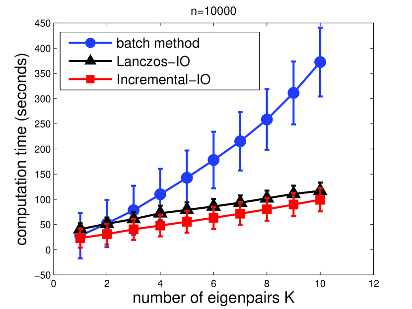
(a)  

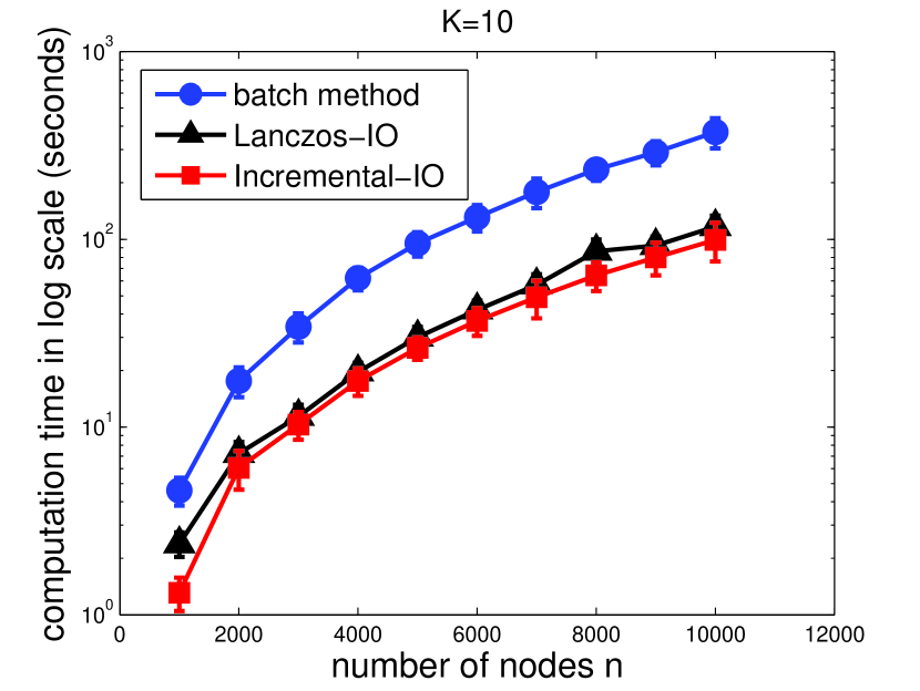
(b)  

Figure 1: Sequential eigenpair computation time on Erdos-Renyi random graphs with edge connection probability $p=0.1$. The marker represents averaged computation time of 50 trials and the error bar represents standard deviation. (a) Computation time with $n=10000$ and different number of eigenpairs $K$. It is observed that the computation time of Incremental-IO and Lanczos-IO grows linearly as $K$ increases, whereas the computation time of the batch method grows superlinearly with $K$. (b) Computation time with $K=10$ and different number of nodes $n$. It is observed that the difference in computation time between the batch method and the two incremental methods grow polynomially as $n$ increases, which suggests that in this experiment Incremental-IO and Lanczos-IO are more efficient than the batch computation method, especially for large graphs.

6.2 Comparison of computation time on real-life datasets

Fig. 2 shows the time improvement of Incremental-IO relative to the batch method for the real-life datasets listed in Table 2, where the difference in computation time is displayed in log scale to accommodate large variance of time improvement across datasets that are of widely varying size. It is observed that the gain in computational time via Incremental-IO is more pronounced as cluster count $K$ increases, which demonstrates the merit of the proposed incremental method.

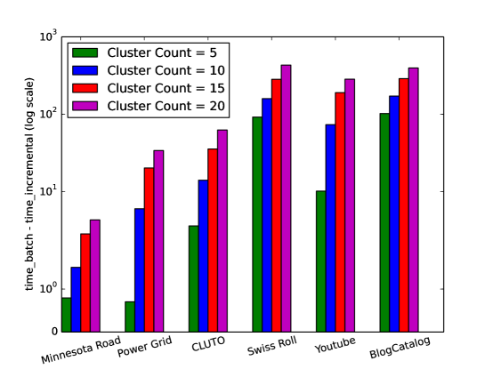
Figure 2: Computation time improvement of Incremental-IO relative to the batch method. Incremental-IO outperforms the batch method for all cases, and has improvement with respect to $K$.

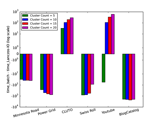
Figure 3: Computation time improvement of Lanczos-IO relative to the batch method. Negative values mean that Lanczos-IO requires more computation time than the batch method. The results suggest that Lanczos-IO is not a robust incremental computation method, as it can perform even worse than the batch method for some cases.

On the other hand, although Lanczos-IO is also an incremental method, in addition to the well-known issue of requiring memory allocation for storing all Lanczos vectors, the experimental results show that it does not provide performance robustness as Incremental-IO does, as it can perform even worse than the batch method for some cases. Fig. 3 shows that Lanczos-IO actually results in excessive computation time compared with the batch method for four out of the six datasets, whereas in Fig. 2 Incremental-IO is superior than the batch method for all these datasets, which demonstrates the robustness of Incremental-IO over Lanczos-IO. The reason of lacking robustness for Lanczos-IO can be explained by the fact that the previously computed Lanczos vectors may not be effective in minimizing the Ritz approximation error of the desired eigenpairs. In contrast, Incremental-IO and the batch method adopt the implicitly-restarted Lanczos method, which restarts the Lanczos algorithm when the generated Lanczos vectors fail to meet the Ritz approximation criterion, and may eventually lead to faster convergence. Furthermore, Fig. 4 shows that Lanczos-IO is overly sensitive to the number of augmented Lanczos vectors $Z_{aug}$, which is a parameter that cannot be optimized a priori.

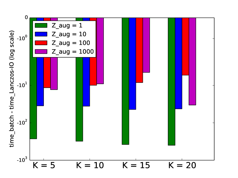
(a) Minnesota Road

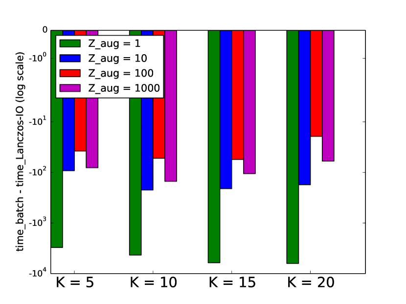
(b) Power Grid

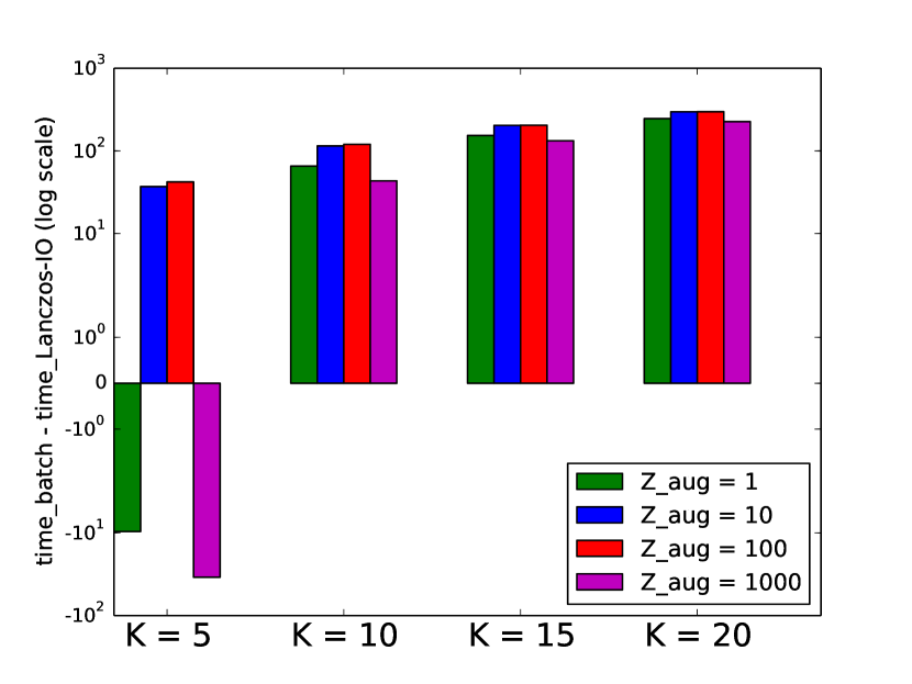
(c) CLUTO

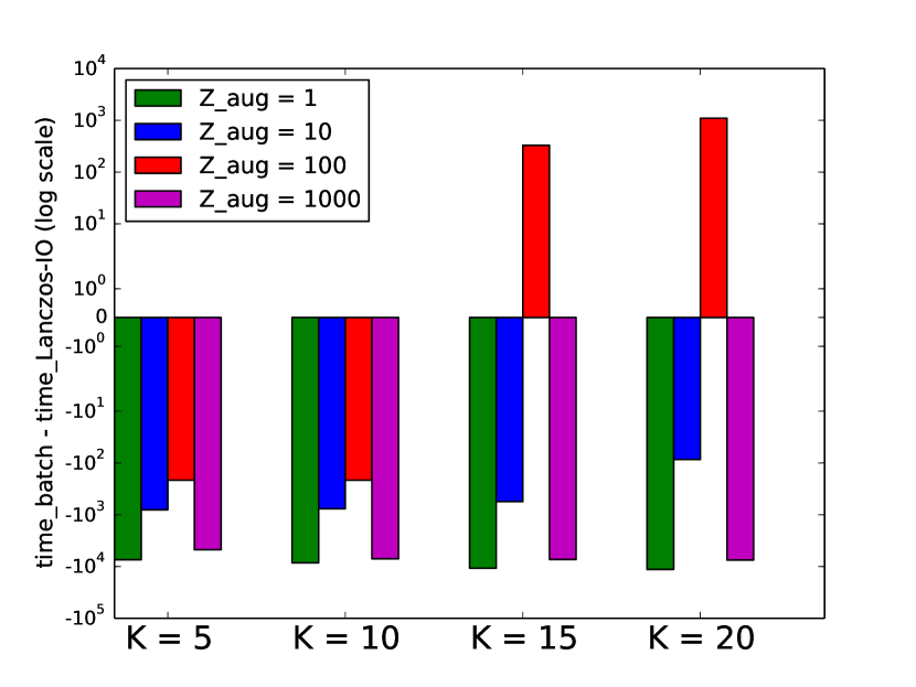
(d) Swiss Roll

(e) Youtube

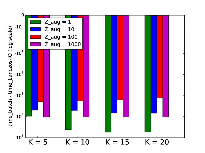
(f) BlogCatalog

Figure 4: The effect of number of augmented Lanczos vectors $Z_{aug}$ of Lanczos-IO in Algorithm 3 on computation time improvement relative to the batch method. Negative values mean that the computation time of Lanczos-IO is larger than that of the batch method. The results show that Lanczos-IO is not a robust incremental eigenpair computation method. Intuitively, small $Z_{aug}$ may incur many iterations in the second step of Algorithm 3, whereas large $Z_{aug}$ may pose computation burden in the first step of Algorithm 3, and therefore both cases lead to the increase in computation time.

Theorem 3.1 establishes that the proposed incremental method (Incremental-IO) exactly computes the $K$-th eigenpair using 1 to $(K-1)$-th eigenpairs, yet for the sake of experiments with real datasets, we have computed the normed eigenvalue difference (in terms of root mean squared error) and the correlations of the $K$ smallest eigenvectors obtained from the batch method and Incremental-IO. As displayed in Fig. 5, the $K$ smallest eigenpairs are identical as expected; to be more specific, using Matlab library, on the Minnesota road dataset for $K=20$, the normed eigenvalue difference is $7\times 10^{-12}$ and the associated eigenvectors are identical up to differences in sign. For all datasets listed in Table 2, the normed eigenvalue difference is negligible and the associated eigenvectors are identical up to the difference in sign, i.e., the eigenvector correlation in magnitude equals to 1 for every pair of corresponding eigenvectors of the two methods, which verifies the correctness of Incremental-IO. Moreover, due to the eigenpair consistency between the batch method and Incremental-IO as demonstrated in Fig. 5, they yield the same clustering results in the considered datasets.

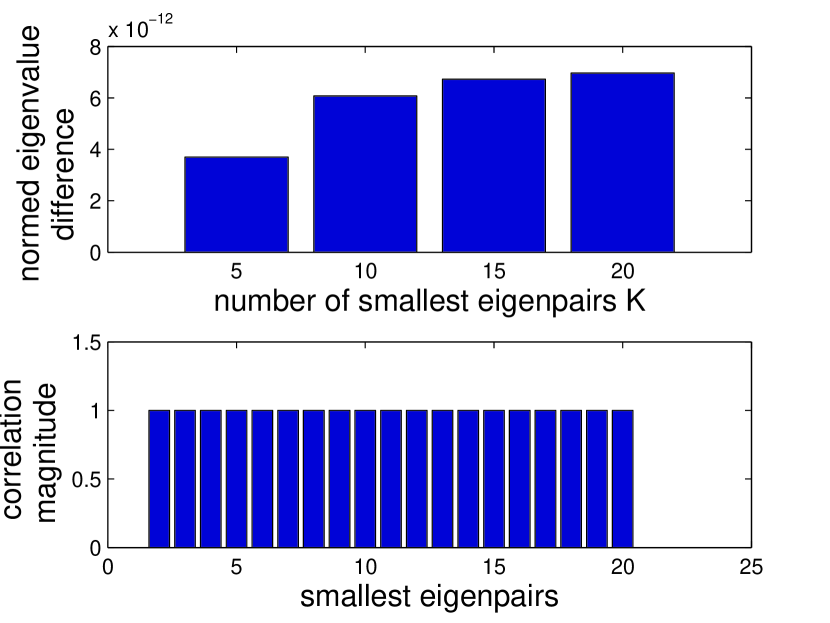
(a) Minnesota Road

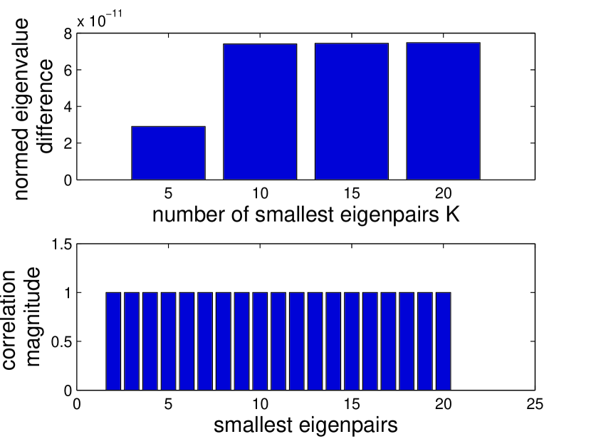
(b) Power Grid

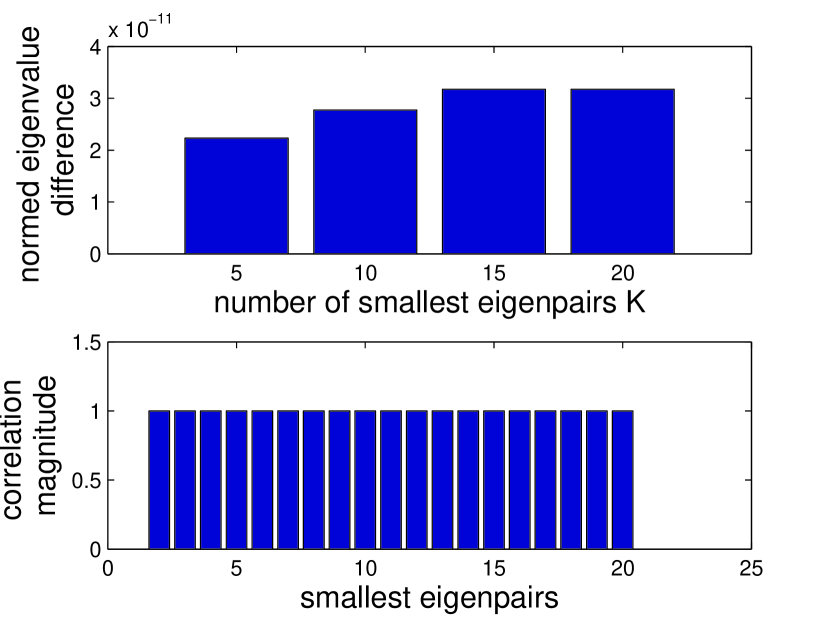
(c) CLUTO

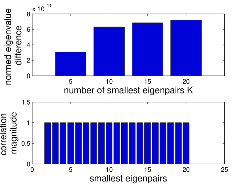
(d) Swiss Roll

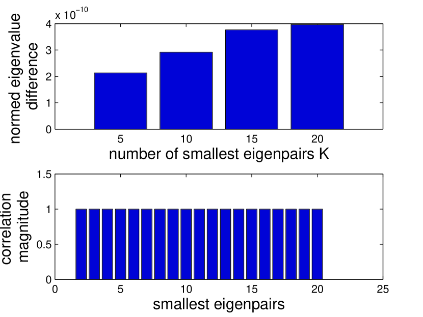
(e) Youtube

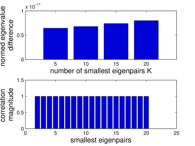
(f) BlogCatalog

Figure 5: Consistency of smallest eigenpairs computed by the batch computation method and Incremental-IO for datasets listed in Table 2. The normed eigenvalue difference is the square root of sum of squared differences between eigenvalues. The correlation magnitude is the absolute value of inner product of eigenvectors, where 1 means perfect alignment.

6.3 Clustering metrics for user-guided spectral clustering

In real-life, an analyst can use Incremental-IO for clustering along with a mechanism for selecting the best choice of $K$ starting from $K=2$. To demonstrate this, in the experiment we use five clustering metrics that can be used for online decision making regarding the value of $K$. These metrics are commonly used in clustering unweighted and weighted graphs and they are summarized as follows.

1. Modularity: modularity is defined as

$$\text{Mod}=\displaystyle\sum_{i=1}^{K}\bigg{(}\frac{W(\mathcal{C}_{i},\mathcal{C}_{i})}{W(\mathcal{V},\mathcal{V})}-\bigg{(}\frac{W(\mathcal{C}_{i},\mathcal{V})}{W(\mathcal{V},\mathcal{V})}\bigg{)}^{2}\bigg{)},$$ (11)

where $\mathcal{V}$ is the set of all nodes in the graph, $\mathcal{C}_{i}$ is the $i$-th cluster, $W(\mathcal{C}_{i},\mathcal{C}_{i})$ ($W(\mathcal{C}_{i},\overline{\mathcal{C}_{i}})$) denotes the sum of weights of all internal (external) edges of the $i$-th cluster, $W(\mathcal{C}_{i},\mathcal{V})=\displaystyle W(\mathcal{C}_{i},\mathcal{C}_{i})+W(\mathcal{C}_{i},\overline{\mathcal{C}_{i}})$, and $W(\mathcal{V},\mathcal{V})=\sum_{j=1}^{n}s_{j}=s$ denotes the total nodal strength.

2. Scaled normalized cut (SNC): NC is defined as Zaki.Jr:14

$$\text{NC}=\displaystyle\sum_{i=1}^{K}\frac{W(\mathcal{C}_{i},\overline{\mathcal{C}_{i}})}{W(\mathcal{C}_{i},\mathcal{V})}.$$ (12)

SNC is NC divided by the number of clusters, i.e., NC/$K$.

3. Scaled median (or maximum) cluster size: Scaled medium (maximum) cluster size is the medium (maximum) cluster size of $K$ clusters divided by the total number of nodes $n$ of a graph.

4. Scaled spectrum energy: scaled spectrum energy is the sum of the $K$ smallest eigenvalues of the graph Laplacian matrix $\mathbf{L}$ divided by the sum of all eigenvalues of $\mathbf{L}$, which can be computed by

$$\text{scaled spectrum energy}=\frac{\sum_{i=1}^{K}\lambda_{i}(\mathbf{L})}{\sum_{j=1}^{n}\mathbf{L}_{jj}},$$ (13)

where $\lambda_{i}(\mathbf{L})$ is the $i$-th smallest eigenvalue of $\mathbf{L}$ and $\sum_{j=1}^{n}\mathbf{L}_{jj}$ $=\sum_{i=1}^{n}\lambda_{i}(\mathbf{L})$ is the sum of diagonal elements of $\mathbf{L}$.

These metrics provide alternatives for gauging the quality of the clustering method. For example, Mod and NC reflect the trade-off between intracluster similarity and intercluster separation. Therefore, the larger the value of Mod, the better the clustering quality, and the smaller the value of NC, the better the clustering quality. Scaled spectrum energy is a typical measure of cluster quality for spectral clustering Polito01grouping ; ng2002spectral ; zelnik2004self , and smaller spectrum energy means better separability of clusters. For Mod and scaled NC, a user might look for a cluster count $K$ such that the increment in the clustering metric is not significant, i.e., the clustering metric is saturated beyond such a $K$. For scaled median and maximum cluster size, a user might require the cluster count $K$ to be such that the clustering metric is below a desired value. For scaled spectrum energy, a user might look for a noticeable increase in the clustering metric between consecutive values of $K$.

6.4 Demonstration

Here we use Minnesota Road data to demonstrate how users can utilize the clustering metrics in Sec. 6.3 to determine the number of clusters. For example, the five metrics evaluated for Minnesota Road clustering with respect to different cluster counts $K$ are displayed in Fig. 6 (a). Starting from $K=2$ clusters, these metrics are updated by the incremental user-guided spectral clustering algorithm (Algorithm 2) as $K$ increases. If the user imposes that the maximum cluster size should be less than $30\%$ of the total number of nodes, then the algorithm returns clustering results with a number of clusters of $K=6$ or greater. Inspecting the modularity one sees it saturates at $K=7$, and the user also observes a noticeable increase in scaled spectrum energy when $K=7$. Therefore, the algorithm can be used to incrementally generate four clustering results for $K=7,8,9$, and $10$. The selected clustering results in Fig. 7 are shown to be consistent with geographic separations of different granularity.

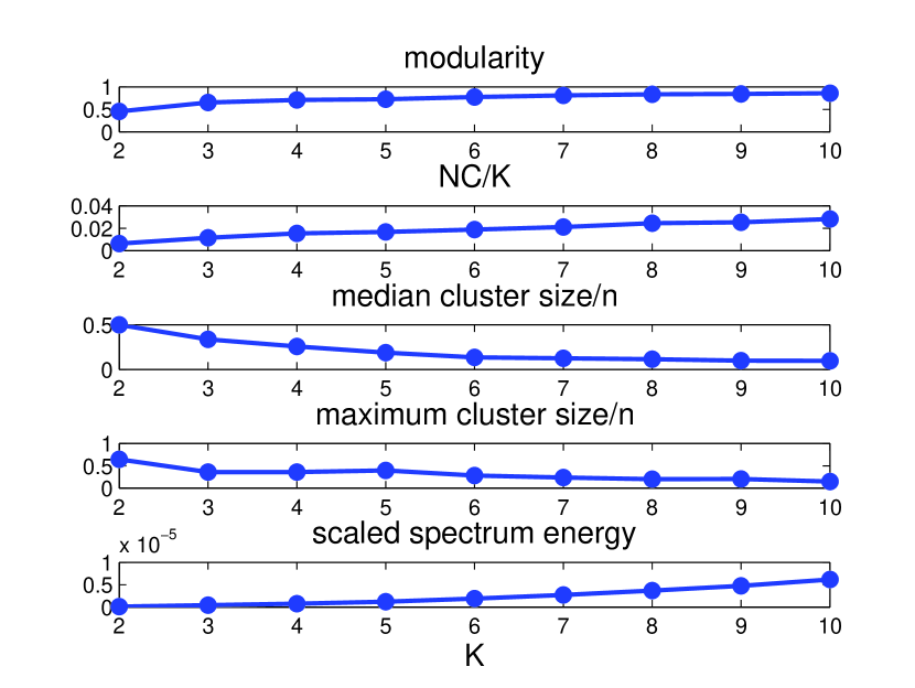
(a) Minnesota Road

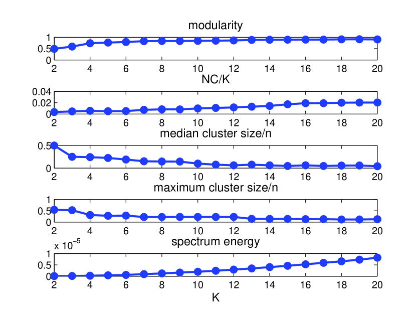
(b) Power Grid

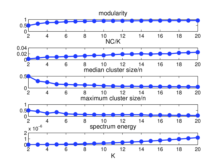
(c) Swiss Roll

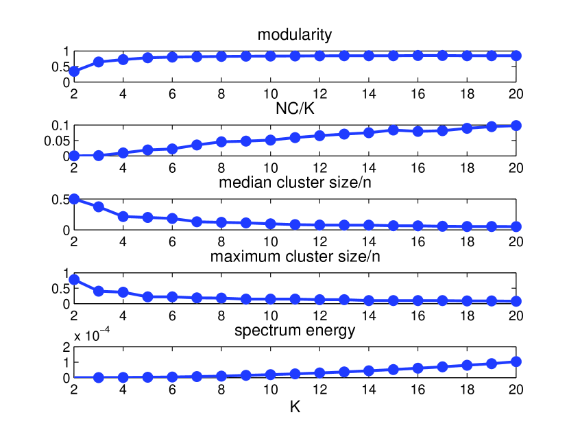
(d) CLUTO

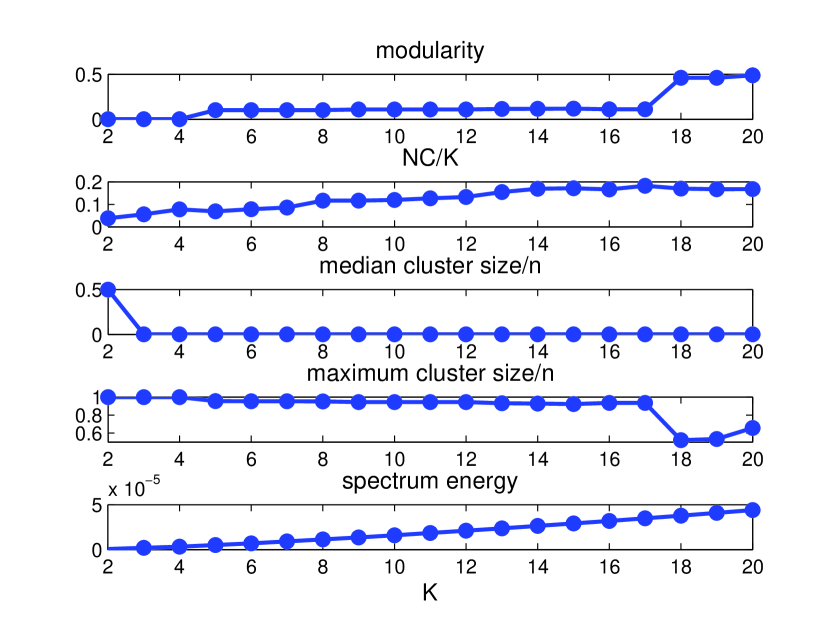
(e) Youtube

(f) BlogCatalog

Figure 6: Five clustering metrics computed incrementally via Algorithm 2 for different datasets listed in Table 2. The metrics are modularity, scaled normalized cut (NC/$K$), scaled median and maximum cluster size, and scaled spectrum energy. These clustering metrics are used to help users determine the number of clusters.

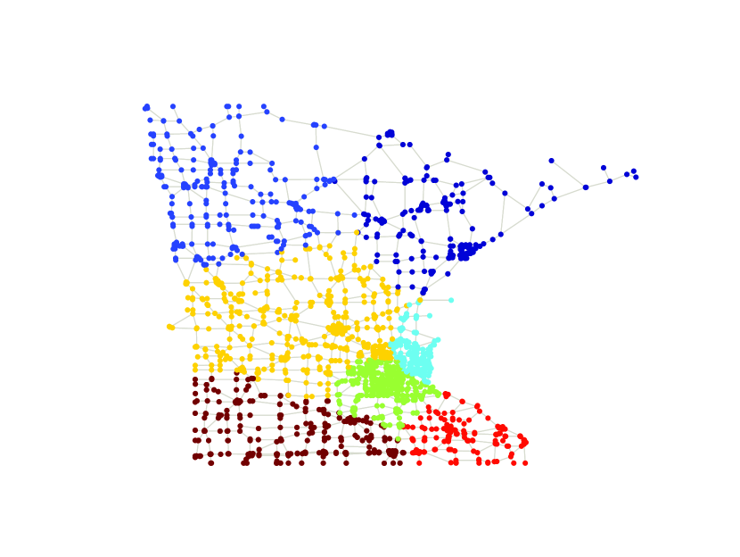
(a) $K=7$

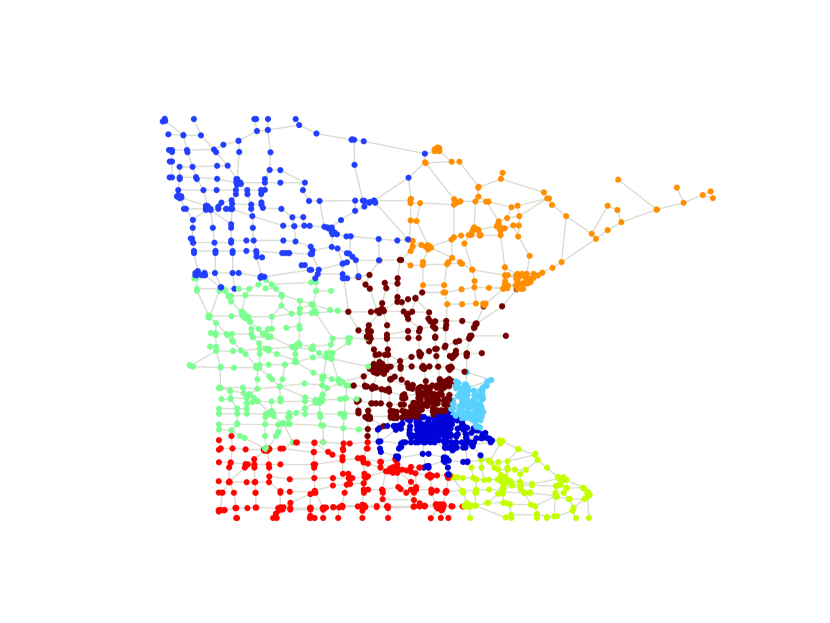
(b) $K=8$

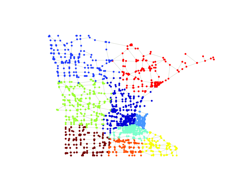
(c) $K=9$

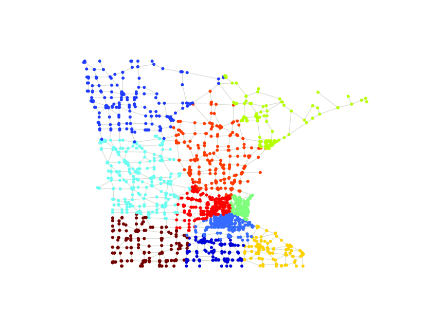
(d) $K=10$

Figure 7: Visualization of user-guided spectral clustering on Minnesota Road with respect to selected cluster count $K$. Colors represent different clusters.

We also apply the proposed incremental user-guided spectral clustering algorithm (Algorithm 2) to Power Grid, CLUTO, Swiss Roll, Youtube, and BlogCatalog. In Fig. 6, we show how the values of clustering metrics change with $K$ for each dataset. The incremental method enables us to efficiently generate all clustering results with $K=2,3,4\ldots$ and so on. It can be observed from Fig. 6 that for each dataset the clustering metric that exhibits the highest variation in $K$ can be different. This suggests that selecting the correct number of clusters is a difficult task and a user might need to use different clustering metrics for a range of $K$ values, and Incremental-IO is an effective tool to support such an endeavor.

7 Conclusion

In this paper we present Incremental-IO, an efficient incremental eigenpair computation method for graph Laplacian matrices which works by transforming a batch eigenvalue decomposition problem into a sequential leading eigenpair computation problem. The method is elegant, robust and easy to implement using a scientific programming language, such as Matlab. We provide analytical proof of its correctness. We also demonstrate that it achieves significant reduction in computation time when compared with the batch computation method. Particularly, it is observed that the difference in computation time of these two methods grows polynomially as the graph size increases.

To demonstrate the effectiveness of Incremental-IO, we also show experimental evidences that obtaining such an incremental method by adapting the existing leading eigenpair solvers (such as, the Lanczos algorithm) is non-trivial and such efforts generally do not lead to a robust solution.

Finally, we demonstrate that the proposed incremental eigenpair computation method (Incremental-IO) is an effective tool for a user-guided spectral clustering task, which effectively updates clustering results and metrics for each increment of the cluster count.

References

- [1] S. Basu, A. Banerjee, and R. J. Mooney. Active semi-supervision for pairwise constrained clustering. In SDM, volume 4, pages 333–344, 2004.
- [2] M. Belkin and P. Niyogi. Laplacian eigenmaps for dimensionality reduction and data representation. Neural computation, 15(6):1373–1396, 2003.
- [3] V. D. Blondel, J.-L. Guillaume, R. Lambiotte, and E. Lefebvre. Fast unfolding of communities in large networks. Journal of Statistical Mechanics: Theory and Experiment, (10), 2008.
- [4] D. Calvetti, L. Reichel, and D. C. Sorensen. An implicitly restarted lanczos method for large symmetric eigenvalue problems. Electronic Transactions on Numerical Analysis, 2(1):21, 1994.
- [5] J. Chen, L. Wu, K. Audhkhasi, B. Kingsbury, and B. Ramabhadrari. Efficient one-vs-one kernel ridge regression for speech recognition. In IEEE International Conference on Acoustics, Speech and Signal Processing (ICASSP), pages 2454–2458, 2016.
- [6] P.-Y. Chen and A. Hero. Deep community detection. 63(21):5706–5719, Nov. 2015.
- [7] P.-Y. Chen and A. Hero. Phase transitions in spectral community detection. 63(16):4339–4347, Aug 2015.
- [8] P.-Y. Chen and A. O. Hero. Node removal vulnerability of the largest component of a network. In GlobalSIP, pages 587–590, 2013.
- [9] P.-Y. Chen and A. O. Hero. Assessing and safeguarding network resilience to nodal attacks. 52(11):138–143, Nov. 2014.
- [10] P.-Y. Chen and A. O. Hero. Phase transitions and a model order selection criterion for spectral graph clustering. arXiv preprint arXiv:1604.03159, 2016.
- [11] P.-Y. Chen and A. O. Hero. Multilayer spectral graph clustering via convex layer aggregation: Theory and algorithms. IEEE Transactions on Signal and Information Processing over Networks, 3(3):553–567, Sept 2017.
- [12] P.-Y. Chen and S. Liu. Bias-variance tradeoff of graph laplacian regularizer. IEEE Signal Processing Letters, 24(8):1118–1122, Aug 2017.
- [13] P.-Y. Chen and L. Wu. Revisiting spectral graph clustering with generative community models. arXiv preprint arXiv:1709.04594, 2017.
- [14] P.-Y. Chen, B. Zhang, M. A. Hasan, and A. O. Hero. Incremental method for spectral clustering of increasing orders. In KDD Workshop on Mining and Learning with Graphs, 2016.
- [15] S. Choudhury, K. Agarwal, S. Purohit, B. Zhang, M. Pirrung, W. Smith, and M. Thomas. NOUS: construction and querying of dynamic knowledge graphs. In Proceedings of 33rd IEEE International Conference on Data Engineering, pages 1563–1565, 2017.
- [16] F. R. K. Chung. Spectral Graph Theory. American Mathematical Society, 1997.
- [17] C. Dhanjal, R. Gaudel, and S. Clémençon. Efficient eigen-updating for spectral graph clustering. Neurocomputing, 131:440–452, 2014.
- [18] M. Dundar, Q. Kou, B. Zhang, Y. He, and B. Rajwa. Simplicity of kmeans versus deepness of deep learning: A case of unsupervised feature learning with limited data. In Proceedings of 14th IEEE International Conference on Machine Learning and Applications, pages 883–888, 2015.
- [19] M. A. Hasan, V. Chaoji, S. Salem, and M. Zaki. Link prediction using supervised learning. In In Proc. of SDM 06 workshop on Link Analysis, Counterterrorism and Security, 2006.
- [20] M. A. Hasan and M. J. Zaki. A Survey of Link Prediction in Social Networks, pages 243–275. Springer US, 2011.
- [21] R. A. Horn and C. R. Johnson. Matrix Analysis. Cambridge University Press, 1990.
- [22] P. Jia, J. Yin, X. Huang, and D. Hu. Incremental laplacian eigenmaps by preserving adjacent information between data points. Pattern Recognition Letters, 30(16):1457–1463, 2009.
- [23] F. Krzakala, C. Moore, E. Mossel, J. Neeman, A. Sly, L. Zdeborova, and P. Zhang. Spectral redemption in clustering sparse networks. Proc. National Academy of Sciences, 110:20935–20940, 2013.
- [24] J. Kuczynski and H. Wozniakowski. Estimating the largest eigenvalue by the power and lanczos algorithms with a random start. SIAM journal on matrix analysis and applications, 13(4):1094–1122, 1992.
- [25] C. Lanczos. An iteration method for the solution of the eigenvalue problem of linear differential and integral operators. Journal of Research of the National Bureau of Standards, 45(4), 1950.
- [26] R. M. Larsen. Computing the svd for large and sparse matrices. SCCM, Stanford University, June, 16, 2000.
- [27] R. B. Lehoucq, D. C. Sorensen, and C. Yang. ARPACK users’ guide: solution of large-scale eigenvalue problems with implicitly restarted Arnoldi methods, volume 6. Siam, 1998.
- [28] S. Liu, H. Chen, S. Ronquist, L. Seaman, N. Ceglia, W. Meixner, L. A. Muir, P.-Y. Chen, G. Higgins, P. Baldi, et al. Genome architecture leads a bifurcation in cell identity. bioRxiv, page 151555, 2017.
- [29] S. Liu, P.-Y. Chen, and A. O. Hero. Accelerated distributed dual averaging over evolving networks of growing connectivity. arXiv preprint arXiv:1704.05193, 2017.
- [30] W. Liu, P.-Y. Chen, S. Yeung, T. Suzumura, and L. Chen. Principled multilayer network embedding. CoRR, abs/1709.03551, 2017.
- [31] W. J. Lu, C. Xu, Z. Pei, A. S. Mayhoub, M. Cushman, and D. A. Flockhart. The tamoxifen metabolite norendoxifen is a potent and selective inhibitor of aromatase (CYP19) and a potential lead compound for novel therapeutic agents. Breast Cancer Research and Treatment, 133(1):99–109, 2012.
- [32] U. Luxburg. A tutorial on spectral clustering. Statistics and Computing, 17(4):395–416, Dec. 2007.
- [33] R. Merris. Laplacian matrices of graphs: a survey. Linear Algebra and its Applications, 197-198:143–176, 1994.
- [34] A. Y. Ng, M. I. Jordan, and Y. Weiss. On spectral clustering: Analysis and an algorithm. In NIPS, pages 849–856, 2002.
- [35] H. Ning, W. Xu, Y. Chi, Y. Gong, and T. S. Huang. Incremental spectral clustering with application to monitoring of evolving blog communities. In SDM, pages 261–272, 2007.
- [36] H. Ning, W. Xu, Y. Chi, Y. Gong, and T. S. Huang. Incremental spectral clustering by efficiently updating the eigen-system. Pattern Recognition, 43(1):113–127, 2010.
- [37] R. Olfati-Saber, J. Fax, and R. Murray. Consensus and cooperation in networked multi-agent systems. 95(1):215–233, 2007.
- [38] B. N. Parlett. The symmetric eigenvalue problem, volume 7. SIAM, 1980.
- [39] Z. Pei, Y. Xiao, J. Meng, A. Hudmon, and T. R. Cummins. Cardiac sodium channel palmitoylation regulates channel availability and myocyte excitability with implications for arrhythmia generation. Nature Communications, 7, 2016.
- [40] M. Polito and P. Perona. Grouping and dimensionality reduction by locally linear embedding. In NIPS, 2001.
- [41] L. K. M. Poon, A. H. Liu, T. Liu, and N. L. Zhang. A model-based approach to rounding in spectral clustering. In UAI, pages 68–694, 2012.
- [42] A. Pothen, H. D. Simon, and K.-P. Liou. Partitioning sparse matrices with eigenvectors of graphs. SIAM journal on matrix analysis and applications, 11(3):430–452, 1990.
- [43] F. Radicchi and A. Arenas. Abrupt transition in the structural formation of interconnected networks. Nature Physics, 9(11):717–720, Nov. 2013.
- [44] G. Ranjan, Z.-L. Zhang, and D. Boley. Incremental computation of pseudo-inverse of laplacian. In Combinatorial Optimization and Applications, pages 729–749. Springer, 2014.
- [45] A. Saade, F. Krzakala, M. Lelarge, and L. Zdeborova. Spectral detection in the censored block model. arXiv:1502.00163, 2015.
- [46] T. K. Saha, B. Zhang, and M. Al Hasan. Name disambiguation from link data in a collaboration graph using temporal and topological features. Social Network Analysis Mining, 5(1):11:1–11:14, 2015.
- [47] J. Shi and J. Malik. Normalized cuts and image segmentation. 22(8):888–905, 2000.
- [48] D. Shuman, S. Narang, P. Frossard, A. Ortega, and P. Vandergheynst. The emerging field of signal processing on graphs: Extending high-dimensional data analysis to networks and other irregular domains. 30(3):83–98, 2013.
- [49] S. M. Van Dongen. Graph clustering by flow simulation. PhD thesis, University of Utrecht, 2000.
- [50] S. White and P. Smyth. A spectral clustering approach to finding communities in graph. In SDM, volume 5, pages 76–84, 2005.
- [51] K. Wu and H. Simon. Thick-restart lanczos method for large symmetric eigenvalue problems. SIAM Journal on Matrix Analysis and Applications, 22(2):602–616, 2000.
- [52] L. Wu, J. Laeuchli, V. Kalantzis, A. Stathopoulos, and E. Gallopoulos. Estimating the trace of the matrix inverse by interpolating from the diagonal of an approximate inverse. Journal of Computational Physics, 326:828–844, 2016.
- [53] L. Wu, M. Q.-H. Meng, Z. Dong, and H. Liang. An empirical study of dv-hop localization algorithm in random sensor networks. In International Conference on Intelligent Computation Technology and Automation, volume 4, pages 41–44, 2009.
- [54] L. Wu, E. Romero, and A. Stathopoulos. Primme_svds: A high-performance preconditioned svd solver for accurate large-scale computations. SIAM Journal on Scientific Computing, 39(5):S248–S271, 2017.
- [55] L. Wu and A. Stathopoulos. A preconditioned hybrid svd method for accurately computing singular triplets of large matrices. SIAM Journal on Scientific Computing, 37(5):S365–S388, 2015.
- [56] L. Wu, I. E. Yen, J. Chen, and R. Yan. Revisiting random binning features: Fast convergence and strong parallelizability. In ACM SIGKDD International Conference on Knowledge Discovery and Data Mining, pages 1265–1274, 2016.
- [57] M. J. Zaki and W. M. Jr. Data Mining and Analysis: Fundamental Concepts and Algorithms. Cambridge University Press, 2014.
- [58] L. Zelnik-Manor and P. Perona. Self-tuning spectral clustering. In NIPS, pages 1601–1608, 2004.
- [59] B. Zhang, S. Choudhury, M. A. Hasan, X. Ning, K. Agarwal, and S. P. andy Paola Pesantez Cabrera. Trust from the past: Bayesian personalized ranking based link prediction in knowledge graphs. In SDM MNG Workshop, 2016.
- [60] B. Zhang, M. Dundar, and M. A. Hasan. Bayesian non-exhaustive classification a case study: Online name disambiguation using temporal record streams. In Proceedings of the 25th ACM International on Conference on Information and Knowledge Management, pages 1341–1350. ACM, 2016.
- [61] B. Zhang, M. Dundar, and M. A. Hasan. Bayesian non-exhaustive classification for active online name disambiguation. arXiv preprint arXiv:1702.02287, 2017.
- [62] B. Zhang and M. A. Hasan. Name disambiguation in anonymized graphs using network embedding. In Proceedings of the 26th ACM International on Conference on Information and Knowledge Management, 2017.
- [63] B. Zhang, N. Mohammed, V. S. Dave, and M. A. Hasan. Feature selection for classification under anonymity constraint. Transactions on Data Privacy, 10(1):1–25, 2017.
- [64] B. Zhang, T. K. Saha, and M. A. Hasan. Name disambiguation from link data in a collaboration graph. In ASONAM, pages 81–84, 2014.