Polarisation in Spin-Echo Experiments: Multi-point and Lock-in Measurements
Abstract
Spin-echo instruments are typically used to measure diffusive processes and the dynamics and motion in samples on ps and ns timescales. A key aspect of the spin-echo technique is to determine the polarisation of a particle beam. We present two methods for measuring the spin polarisation in spin-echo experiments. The current method in use is based on taking a number of discrete readings. The implementation of a new method involves continuously rotating the spin and measuring its polarisation after being scattered from the sample. A control system running on a microcontroller is used to perform the spin rotation and to calculate the polarisation of the scattered beam based on a lock-in amplifier. First experimental tests of the method on a helium spin-echo spectrometer, show that it is clearly working and that it has advantages over the discrete approach i.e. it can track changes of the beam properties throughout the experiment. Moreover, we show that real-time numerical simulations can perfectly describe a complex experiment and can be easily used to develop improved experimental methods prior to a first hardware implementation.
I Introduction
Spin-echo instruments provide unique information about the dynamics and motion of atoms, molecules and macromolecular objectsMezei, Knaak, and Farago (1987); Frick and Richter (1995); Swenson, Bergman, and Longeville (2001); Richter et al. (2005); Alexandrowicz and Jardine (2007); Jardine et al. (2009); Hedgeland et al. (2009); Fouquet, Hedgeland, and Jardine (2010); Tamtögl et al. (2018): Upon inelastic scattering from a sample the initial polarisation of a polarised beam is changed. The phase shift of the scattered beam includes important information about the sample dynamics. Hence one of the key aspects of the spin-echo technique is to determine the polarisation of a particle beam. Typically this is done by measuring a couple of discrete points while scanning around the echo conditionDeKieviet et al. (1995); Mezei, Pappas, and Gutberlet (2003). In this work we present two methods, the above described discrete sampling and a new method based on a continuous spin rotation, in the framework of helium spin-echo spectroscopy.
Helium Spin-Echo (HeSE) spectroscopy is a novel technique which combines the surface sensitivity and the inert, completely non-destructive nature of helium atom scatteringFarías and Rieder (1998); Benedek and Toennies (1994); Kraus et al. (2013) with the unprecedented energy resolution of the spin-echo methodDeKieviet et al. (1995); Gähler et al. (1996); Mezei, Pappas, and Gutberlet (2003); Fouquet, Hedgeland, and Jardine (2010). It allows the study of surface dynamics over time-scales down to sub-picoseconds with atomic resolutionAlexandrowicz and Jardine (2007); Jardine et al. (2009). The apparatus has previously been used to measure diffusion on surfacesHedgeland et al. (2009); Bahn et al. (2017), surface phonon spectraTamtögl et al. (2015, 2017) and ultra-high resolution potential energy landscapes Jardine et al. (2004). The polarisation of the He beam is measured by taking a number of discrete points (four) during an echo-scan. We begin by considering this four-point method and note that it suffers from the need for a separate calibration of beam energy and that it also assumes the beam energy is stable throughout the experiment. Starting with a numerical model we show that a new method is capable of monitoring the polarisation continuously. Preliminary experiments using a microcontroller based hardware show clearly that the method works and has advantages over the conventional discrete approach: It requires no initial calibration and adapts to changing conditions.
II Experimental Setup
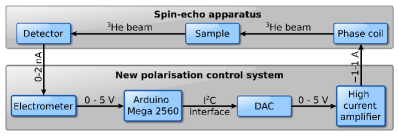
In order to perform HeSE measurements, helium-3 (3He) is used which has a non-zero nuclear magnetic moment (spin). The spin is aligned perpendicular to the beam axis, and in the Cambridge instrument scattered of the sample surface in a fixed 44.4∘ source-target-detector geometry. A schematic of the 3He spin-echo apparatus is illustrated in Figure 1 (with the 44.4∘ scattering geometry removed for simplicity) which shows the important componentsFouquet et al. (2005).
A nearly monochromatic beam of 3He is generated with the velocity along the -direction. The beam passes through a spin polariser, where the nuclear spin is polarised perpendicular to the beamline (along ). Before reaching the sample, the beam passes through a magnetic field parallel to the beam axis, which is generated by the incoming solenoid. Thus, the spins perform a Larmor precession in the plane where the angle between the 3He spin before and after passing the solenoid depends on the time spent in the magnetic field and hence on its velocity. The 3He beam is then scattered from the sample and travels through the outgoing solenoid which creates a magnetic field with an amplitude usually equal to that of the incoming coil but now directed anti-parallel to the beam axis. Hence the Larmor precession unwinds the spin so that the spin direction at the end of the outgoing coil is the same as at the beginning of the incoming coil (along the -direction) provided that the scattering event is purely elastic. Finally, the analyser only selects components of the beam with the spin aligned along after which a detector converts the flux of 3He into a count rate.
After inelastic or quasi-elastic scattering from the sample surface due to dynamical processes, the signal will only be partially polarised. Consequently, a crucial part of these experiments is to determine the polarisation of the scattered beam.
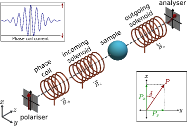
The phase coil is included before the incoming solenoid and allows the spin to be rotated by an additional chosen amount. The top left inset illustrates the spin polarisation versus the phase coil current for purely elastic scattering. The phase coil is used to determine both the real and the complex part of an arbitrary spin polarisation in the plane (see the inset at the bottom right).
III Polarisation measurement
By measuring how the polarisation changes with increasing current through the solenoids the dynamic properties of the sample can be found. An arbitrary polarisation of the spin in the -plane can be conveniently written as a complex number,
| (1) |
where and (see also the illustration in the inset of Figure 1). In principle it is not essential to measure both and in every experiment. E.g. a measurement of gives the real part of the intermediate scattering function . However, some inelastic processes such as phonon events require the measurement of both components of the polarisationJardine et al. (2009).
Moreover, even without a magnetic field in the solenoids () the polarisation may not be entirely real due to practical hardware implementations. These include the misalignment of magnetic elements, small differences between the two coils and their driving circuits as well as external magnetic fields penetrating the beam path. The issue is illustrated in Figure 2 which shows schematically a line corresponding to a polarisation measurement under ideal conditions (black, dashed) and a realistic elastic measurement (blue, solid). Hence to obtain the maximum amplitude of the polarisation (due to practical limitations of the apparatus) and the complete information about the underlying dynamical processes both the real and the imaginary part of the polarisation need to be measured.
In principle the simplest way of measuring the complex polarisation is to rotate the analyser (in Figure 1), by which allows independent measurements of the polarisation along the and the -axis: and . However, mechanical rotations of magnetic devices on the instrument are quite complicated and in practice there are simpler solutions. The most convenient approach is to add an additional “phase coil” in the region before the incoming solenoid (see Figure 1). The phase coil rotates the spin by a chosen amount depending on the magnetic field . Thus the ingoing spin vector can be rotated with respect to the outgoing one by a certain amount which is determined by the current through the phase coil. By measuring a number of discrete points within the period of one full spin rotation the exact polarisation of the spin can be measured. In neutron spin-echo spectroscopy this is typically termed as measurement of the echo-group or as so-called echo-scanMezei, Pappas, and Gutberlet (2003); Farago (2003); Ohl et al. (2012). The process is illustrated for four points in Figure 2 and will be described in the following.
III.1 The 4-Point Measurement
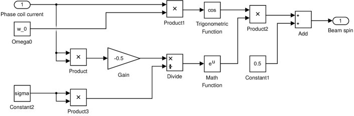
As described in the previous section, the complex polarisation of the beam can be measured via an additional spin rotation in the phase coil. With a current, , passing through the phase-coil, a spin is rotated through an angle where the rotation constant , depends on the mean wavelength of the particles in the beam, , the particle mass and the field integral along the beam path Jardine et al. (2009); Alexandrowicz and Jardine (2007); Jones et al. (2016). The signal resulting from a fixed polariser in the case of a beam with a Gaussian spread of wavelengths is derived in the Supplementary Information and is
| (2) |
In practice the polarisation is measured via the 3He atoms that arrive at the detector where the flux is converted into a count rate
| (3) |
The count rate in the detector follows (3) as the current in the phase coil () is changed (see Figure 2). The term describes the rotation of the spin and is determined by the mean wavelength of the particles (via ) and the current through the phase coil. The phase shift in (3) accounts for non-idealities within the ingoing and outgoing spin rotation as discussed above: It describes the effect that the polarisation is not entirely real for as illustrated in the upper panel of Figure 2. The spread of wavelengths in the beam is manifest through the Gaussian pre-factor in (3), of width , where is the corresponding spread in wavelengths.
Finally, the offset in (3) is composed of a background in the detector and an offset which is due to the fact that the polarisation of the 3He beam and the selection of a single polarisation by the analyser cannot be perfect in reality.
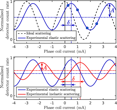
Lower panel: The red solid line illustrates an inelastic scattering experiment where motion gives rise to an additional phase shift and a change in the amplitude of the signal with respect to scattering from a static sample (blue curve).
The properties of the beam and in (3) have typically been determined beforehand. When there is little time variation of and the beam properties may be determined in an infrequent precise measurement over many oscillations. The process involves a measurement of the polarisation for a static sample while scanning the current in the incoming solenoid with the outgoing solenoid current held at zero. At present, the measurement takes about 20 min to perform and is usually done each time the beam is adjustedWard (2013). The polarised intensity is then measured for a number of different phase coil currents in a single period of the oscillation, as shown by the example blue markers in Figure 2 which is then used to calculate the complex polarisation of the beam.
Hence if the properties of the beam are known, there are three remaining variables in (3): , and . These variables can be determined by measuring at three different phase coil currents over one oscillation period and solving the resulting set of linear equations. In practice we measure 4 points as described above giving rise to an over constrained set of linear equations which is solved using a least squared optimisation. The measurement of four points presents a balance of accurate results and high throughput.
Finally after all variables have been determined, (3) can be used to calculate the real and the complex part, and of the spin polarisation. Any changes of the polarisation due to dynamical processes can be determined using this principle. In general, quasi-elastic and inelastic scattering off the sample gives rise to a change of the phase and amplitude of the oscillation with respect to an elastic scattering event, which is illustrated in the lower panel of Figure 2.
III.2 The Spin-Rotator Method
The conventional method of measuring the polarisation, the four point method described in the previous section, involves passing discrete currents through the phase coil, each rotating the direction of the spin by a different amount and measuring the scattered signal at the detector. Even though this method has proven to be perfectly suitable for most measurements it exhibits a couple of disadvantages. Firstly, the calibration routine used at the start is relatively time consuming ( min). Then four data points are used to find three parameters which means the system is susceptible to noise, e.g. fluctuations in the detector. Finally it is assumed that the value of and remain constant throughout the experiment. In the following we present a new method of finding the polarisation which does not require initial calibration, is less susceptible to noise and will adjust to changing values of and .
The proposed new method involves continuously rotating the polarisation of the incoming beam instead of rotating it by separate discrete amounts. In doing so, the polarised component will cause an oscillating signal in the detector where the frequency of the oscillation equals the frequency of the spin rotation. Any remaining unpolarised component will give rise to a constant D.C. level in the detector.
Hence a lock-in amplifier with the same frequency as the spin rotation can be used to extract the polarised component of the signal (see section S3.A in the supplementary information and Caldwell (1977) for a similar concept in the context of polarisation measurements in optical systems). The unpolarised component can be found by running the detector signal through a low pass filter. Using both components the magnitude of the polarisation and the phase of the spin can be calculated. The method has the advantage of requiring no initial calibration while also taking data continuously.
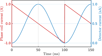
In order to rotate the initial spin direction continuously, the current in the phase coil needs to be linearly increased. To obtain this effect with a finite current, the current is first increased linearly and then quickly dropped back to the starting current (a sawtooth wave). If the amplitude is chosen correctly, at the start of each period the 3He beam will have the same polarisation direction as at the end of the previous period. Figure 3 illustrates that this will create a smooth sine wave at the detector, based on a numerical simulation with an idealised model of the system (which will be discussed below).
If the amplitude is incorrect, there will be a sudden jump in the signal at the end of each period. The correct amplitude is ensured by controlling the amplitude of the modulating sawtooth with feedback from the detector output. Figure 4 shows a block diagram of the new method for the polarisation measurement with the feedback loop in red. The output from the detector passes through a lock-in amplifier with a reference signal at which controls the amplitude of the sawtooth. Starting with an arbitrary initial amplitude of the sawtooth current in the phase coil, the system should tend towards a stable position where the phase coil amplitude corresponds to one complete rotation of the 3He spin. We will discuss this in more depth on the basis of a numerical model of the system below.
IV Numerical Model
A numerical model allows the behaviour of the system to be tested. Starting with an idealised system to check the feasibility of the method it permits the subsequent addition of imperfections of a realistic system step by step so that the effect of each can be found. Simulink (a graphical programming language for modelling dynamic systems) was chosen to model the system as it enables rapid production of a simple model which can then easily be modified with more realistic aspects.
IV.1 An Idealised Numerical Model
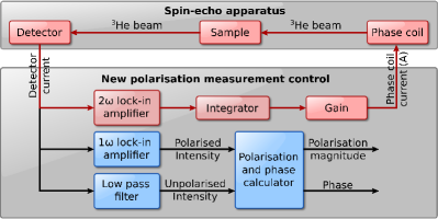
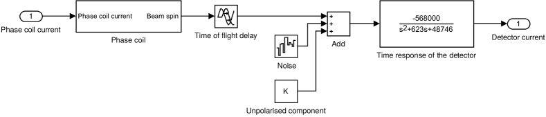
The behaviour of the aforementioned new method of polarisation measurements was first modelled in Simulink using the components shown in Figure 4. We have already seen in Figure 3 that the right choice of the sawtooth amplitude in the phase coil gives rise to a sinusoidal current output from the detector. However, the system should find the right amplitude starting from an arbitrary initial value. Therefore a feedback loop (red parts in Figure 4) consisting of a lock-in amplifier, an integrator and the feedback loop gain is used. The spin-echo machine and the current output from the detector is modelled to follow equation (3).
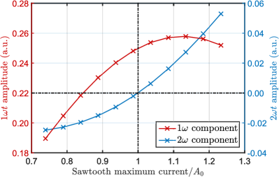
Figure 5 shows that a non-perfect amplitude introduces higher Fourier components to the signal. At the perfect amplitude, the signal at twice the sawtooth frequency (2) goes to zero as expected. To ensure that the amplitude is kept at the correct value, a system of negative feedback can be used as the signal changes sign at the perfect amplitude (vertical dash-dotted line in Figure 5).
The feedback loop is created by integrating the component to give it an infinite DC gain and to act as the dominant pole in the loopPippard (1985). The integrated signal is multiplied by an adjustable constant, known as the feedback gain and then multiplied by a unit amplitude sawtooth wave to supply the current in the phase coil. Finally, a lock-in amplifier and a low pass filter provide the polarised and unpolarised components of the signal, respectively, which are used to calculate the magnitude of the polarisation and the phase (see Figure 4).
IV.2 A Realistic Numerical Model
The model described above assumes an ideal system which corresponds instantaneously to any changes and is free from any background noise. As a more realistic model, three sources of imperfection were added:
-
•
Background noise.
-
•
The continuous change of current in the phase coil compared to the ideal instantaneous jump: Due to the inductance of the phase coil the rapid change of current at the end of the sawtooth period (Figure 3) will not be instantaneous. Instead the current will change continuously and during this time, the spin polarisation is rotated by a full cycle very quickly leading to a short blip in the detector current. This blip will give rise to frequency components across the whole spectrum but it will not affect the stability of the system as shown by tests with the realistic model and also in the measurements later.
-
•
The response function of the apparatus consisting of the time-of-flight of the 3He atoms and the response of the detector.
The last point is also interesting from an experimental point of view and has not been determined previously. Hence we will discuss it in the next section. The setup of the Simulink model itself can be found in the Supplementary Information.
IV.3 Apparatus Response Function
After the field in the phase coil is changed, the 3He atom must travel the length from the phase coil to the detector where it is ionised and then converted to a count rate, meaning the response is not instantaneous. Since the 3He atoms do not interact with each other, a linear response function represents a good model of the machine.
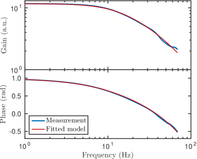
The frequency response of the apparatus was determined by applying a square wave of fixed frequency to the phase-coil. The current in the phase-coil and the detector count rate were both measured and Fourier transforms of both were taken, they were then used to calculate the gain and phase shift as a function of frequency. The response determined from the upward transition of the square wave was identical to that from the downward transition, confirming the linearity of the system. An average over several cycles leads to the frequency response shown in Figure 6 (blue lines).
A transfer function of the form, Equation 4, was fitted to the measured data where is the Laplace transform variable and is a time delay due to the time-of-flight.
| (4) |
Equation 4 has a gain and phase according to
| (5) | ||||
The gain was fitted first since it is most sensitive to changes in , and the . Once a fit for that had been found, the value of was fitted for the phase. The values of the fitted parameters are summarised in Table 1 and the fitted response, plotted in red in Figure 6, shows a good agreement between the measurement and the model.
| Parameter | Value |
|---|---|
| Hz | |
| Hz | |
| ms |
The parameter is expected to be the time delay due to the time-of-flight of the 3He atom from the phase coil to the detector. The length of this section of the machine is known fromJardine et al. (2009) ( m) which would give a time-of-flight of ms for an 8 meV 3He beam. This value agrees very well with the value obtained from the measurement (Table 1), indicating that the time-of-flight is indeed the dominant contribution to the delay. Note that the gain obtained from the measurement will change from experiment to experiment since it depends on properties such as the beam intensity and the reflectivity of the sample.
The poles of the response function correspond to time constants of approximately 10 ms and 2 ms; these are due to the diffusion and ionisation time scales within the detector respectively. It is important to bear these in mind when choosing the frequency at which the system should run at. Above these poles, phase changes occur which may change negative feedback to positive feedback and the gain starts to decrease, reducing the measurable signal, but as the frequency is lowered, the system will respond slower to any changes. In the following experiments a frequency of 5 Hz was used.
IV.4 Closed Loop Response of the Realistic Model
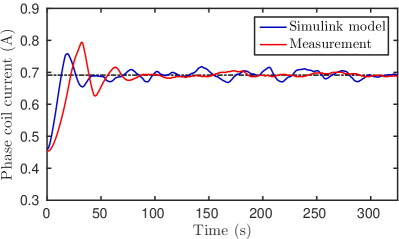
Red line: The behaviour of the hardware version of the polarisation control system tracked by measuring the maximum current through the “real” phase coil. The system shows similar behaviour to the realistic model.
The stability of the realistic numerical model was tested by tracking the amplitude of the sawtooth throughout the experiment. Starting with an arbitrary initial amplitude the system should then tend towards the ideal amplitude which corresponds to exactly one rotation of the spin. Therefore the maximum amplitude of the current in the phase coil is monitored versus time, which is shown in Figure 7. The horizontal dash-dotted line illustrates the theoretical perfect amplitude based on the beam energy and solenoid properties.
The system follows a typical negative feedback behaviour: The amplitude tends to the theoretical correct value, overshoots slightly before oscillating with decaying amplitude around the perfect value. The time delay and response function for the detector had no noticeable effect on whether the system was stable for a range of lock-in amplifier time constants and feedback gains. However, the realistic system tends to oscillate around the constant value with a higher frequency and higher amplitude compared to the idealised model. Size/frequency of these oscillations can be changed by optimising the parameters of the feedback loop (gain, time constant)Taylor (1994).
V Hardware Implementation
Since the model showed that it is theoretically possible to measure the polarisation with the new method a hardware version was implemented which can be connected to the spin-echo machine. In order to do this, the Simulink program which controls the feedback and calculates the polarisation needs to run in real time. It also needs to drive the current through the phase coil and read the current from the detector back in.
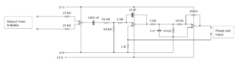
The control system was chosen to run on a microcontroller, an Arduino Mega 2560. It has enough internal memory to store the required programme, can send and receive data through a high speed I2C interface and can send data to a PC for logging purposes. For the typical beam energies of the apparatus ( meV) a maximum current of 0.9 A through the phase coil is required to guarantee a full spin rotation at the highest energy beam. Therefore the Arduino is connected to a 12 bit digital to analogue converter (DAC, MCP4725) via the I2C interface. The V of the DAC are then used to provide the phase coil current via a high current amplifier (see Supplementary Information for the circuit diagrams). Thus a range of A to A through the phase coil is achieved, which meets the standard conditions and also gives some space for overshoots of the sawtooth wave.
The built-in analogue input on the Arduino was used to read the detector current. Since the output from the detector varies between and A, a simple electrometer converts the current into a V output. For a first test it was decided to focus on the middle range (1 nA range). A block diagram of the final setup is shown in Figure 8.
VI Experimental Results
To test the apparatus on the spin echo machine a graphene/Ni(111) surface was usedTamtögl et al. (2015) with the scattering slightly off specular. This arrangement was chosen since it gives a detector current in the desired range as well as a partly polarised scattered beam. The process was monitored by recording the current though the phase coil and the current in the detector, simultaneously, via an oscilloscope (see Supplementary Information for more details).
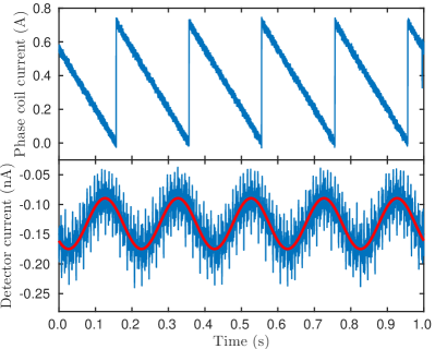
After the system has reached stability the current measured in the phase coil (top panel of Figure 9) shows the expected sawtooth shape and the current from the detector (bottom panel of Figure 9) shows a definite sine wave. The red curve in Figure 9 is a sine fit to the detector current. The frequency of the sine wave is 5 Hz indicating that the system has successfully locked in and that the concept is working.
The measured signal exhibits still a large fraction of noise which is mainly due to the simple setup of the electric circuits for reading in the detector current. Nevertheless, the first test shows that the spin-rotator method is perfectly working and we will discuss its advantages over the 4-point method at the end of this section. Furthermore, the test also shows that a lock-in amplifier can be easily implemented and run on a microcontroller, similar in spirit to previous worksGonzàlez et al. (2007); Schultz (2016).
The stability of the system can be tested in the same manner as the numerical model. Therefore, the maximum amplitude of the phase coil current is plotted in red in Figure 7. After the system has been switched on with an initial amplitude that is much smaller than the perfect amplitude it again overshoots before it oscillates slightly around the perfect amplitude. The amplitude has stabilised within less than a minute. The comparison with the numerical model (Figure 7) shows that the similarity between the real system and the model is remarkable.
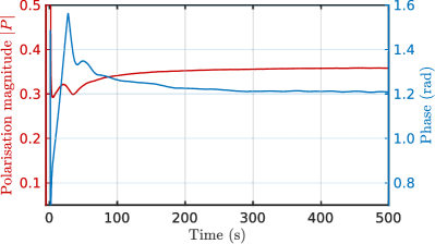
These experiments had all shown the system to be stable so the next test was to try taking a measurement of the beam polarisation. The polarisation and phase can be seen in Figure 10 to tend to a stable polarisation of . Note that the maximum polarisation of the 3He beam is due to the polariser and transmission properties of the apparatusMcIntosh et al. (2018). Hence this corresponds to a polarisation of roughly 60% for the scattered 3He beam. The uncertainty of the measured polarisation shows a factor of three improvement with the new method compared to the 4-point measurement. The measurement of the phase settled on a constant value with fluctuations of 0.0018 rad, again the four-point method did not measure the phase to an accuracy of 0.004 rad. On the other hand, a direct comparison with the four-point method is difficult to make, since the system started from an arbitrary initial value and the measurement was taken after a longer time.
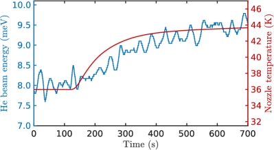
The ability to monitor polarisation continuously is a significant advantage of the spin-rotator method. As mentioned in subsection III.1, the 4-point measurement assumes a constant beam profile throughout a run of experiments. The behaviour of the new polarisation control system with respect to this aspect can be tested by actively changing the beam properties, i.e. by changing the helium beam energy. The beam energy is determined by the temperature of the nozzle , which produces the atomic beam, via . Here, is the Boltzmann constantFarías and Rieder (1998). Note however, that the nozzle temperature cannot be used for an exact measurement of the beam energy since there might be small differences between the diode-based temperature measurement and the actual temperature inside the nozzleLechner et al. (2013).
The blue curve in Figure 11 shows the beam energy calculated from the output voltage of the microcontroller. The red curve in Figure 11 displays the nozzle temperature which is proportional to the 3He beam energy. Starting with a nozzle temperature of 36 K, after about 150 s the nozzle temperature starts to increase, from about 8 to 9.5 meV. The amplitude of the sawtooth has to increase with increasing beam energy in order to maintain a full spin rotation in the phase coil. While there are still small oscillations on the beam energy determined from the control system, it definitely follows the general trend of the nozzle temperature. Hence the new system is stable regardless of the beam energy and can track changes of the beam properties throughout the experiment.
In cases where the beam polarisation is negligible for an extended period it is likely that the simple integrator in the feedback loop (Figure 4) will cause the amplitude of the current in the phase-coil to drift. The feedback loop will restore the correct amplitude as soon as the polarisation returns. However, if the drift is problematic it would be straightforward to add a sample/hold element controlled by the polarisation magnitude so that the feedback loop is inhibited and the phase-coil amplitude fixed, whenever the polarisation falls below a certain pre-set value.
VII Summary and Conclusion
In summary, we have described two methods of measuring the polarisation in spin-echo experiments: The four-point method, which is based on taking discrete points along an echo scan and a new, so called spin-rotator method. Numerical simulations and a novel hardware implementation have been used to develop the new method which involves rotating the spin and measuring its polarisation after scattering continuously. A control system implemented on a microcontroller is used to control the spin rotation and to calculate the polarisation of the scattered beam, based on a lock-in amplifier.
First experimental tests of the new method on a helium spin-echo apparatus show clearly that the method is working. While the first hardware implementation of the spin-rotator method may still require a number of improvements in terms of noise reduction and speed, the first tests show that it has advantages over the conventional discrete approach. The four-point method, which is currently used, requires a preceding calibration at the start of an experiment and assumes a constant beam profile. The spin-rotator method, on the other hand, does not assume a constant beam profile and can track changes of the beam properties throughout the experiment.
Moreover, our numerical model shows, that real-time numerical simulations are capable of accurately describing a complex experiment. They can be used to test the behaviour and viability prior to first experiments. Finally, our tests show that a lock-in amplifier can be simply implemented on a cheap microcontroller and perform the tasks of a bench-top lock-in amplifier.
Supplementary Material
The setup of the numerical model in Simulink and the circuit diagrams of the hardware implementation can be found in the supplementary material.
Acknowledgement
One of us (A.T.) acknowledges financial support provided by the FWF (Austrian Science Fund) within the project J3479-N20.
References
- Mezei, Knaak, and Farago (1987) F. Mezei, W. Knaak, and B. Farago, Phys. Rev. Lett. 58, 571 (1987).
- Frick and Richter (1995) B. Frick and D. Richter, Science 267, 1939 (1995).
- Swenson, Bergman, and Longeville (2001) J. Swenson, R. Bergman, and S. Longeville, J. Chem. Phys 115, 11299 (2001).
- Richter et al. (2005) D. Richter, M. Monkenbusch, A. Arbe, and J. Colmenero, Neutron Spin Echo in Polymer Systems, Advances in Polymer Science, Vol. 174 (Springer Berlin Heidelberg, Berlin, Heidelberg, 2005) pp. 1–221.
- Alexandrowicz and Jardine (2007) G. Alexandrowicz and A. P. Jardine, J. Phys.: Cond. Matt. 19, 305001 (2007).
- Jardine et al. (2009) A. Jardine, H. Hedgeland, G. Alexandrowicz, W. Allison, and J. Ellis, Prog. Surf. Sci. 84, 323 (2009).
- Hedgeland et al. (2009) H. Hedgeland, P. Fouquet, A. P. Jardine, G. Alexandrowicz, W. Allison, and J. Ellis, Nat. Phys. 5, 561 (2009).
- Fouquet, Hedgeland, and Jardine (2010) P. Fouquet, H. Hedgeland, and A. P. Jardine, Z. Phys. Chem 224, 61 (2010).
- Tamtögl et al. (2018) A. Tamtögl, M. Sacchi, I. Calvo-Almazán, M. Zbiri, M. M. Koza, W. E. Ernst, and P. Fouquet, Carbon 126, 23 (2018).
- DeKieviet et al. (1995) M. DeKieviet, D. Dubbers, C. Schmidt, D. Scholz, and U. Spinola, Phys. Rev. Lett. 75, 1919 (1995).
- Mezei, Pappas, and Gutberlet (2003) F. Mezei, C. Pappas, and T. Gutberlet, Neutron spin echo spectroscopy: basics, trends, and applications, Lecture notes in physics No. 601 (Springer, Berlin ; New York, 2003).
- Farías and Rieder (1998) D. Farías and K.-H. Rieder, Rep. Prog. Phys. 61, 1575 (1998).
- Benedek and Toennies (1994) G. Benedek and J. P. Toennies, Surf. Sci. 299, 587 (1994).
- Kraus et al. (2013) P. Kraus, A. Tamtögl, M. Mayrhofer-Reinhartshuber, G. Benedek, and W. E. Ernst, Phys. Rev. B 87, 245433 (2013).
- Gähler et al. (1996) R. Gähler, R. Golub, K. Habicht, T. Keller, and J. Felber, Physica B Condens Matter. 229, 1 (1996).
- Bahn et al. (2017) E. Bahn, A. Tamtögl, J. Ellis, W. Allison, and P. Fouquet, Carbon 114, 504 (2017).
- Tamtögl et al. (2015) A. Tamtögl, E. Bahn, J. Zhu, P. Fouquet, J. Ellis, and W. Allison, J. Phys. Chem. C 119, 25983 (2015).
- Tamtögl et al. (2017) A. Tamtögl, P. Kraus, N. Avidor, M. Bremholm, E. M. J. Hedegaard, B. B. Iversen, M. Bianchi, P. Hofmann, J. Ellis, W. Allison, G. Benedek, and W. E. Ernst, Phys. Rev. B 95, 195401 (2017).
- Jardine et al. (2004) A. P. Jardine, S. Dworski, P. Fouquet, G. Alexandrowicz, D. J. Riley, G. Y. H. Lee, J. Ellis, and W. Allison, Science 304, 1790 (2004).
- Fouquet et al. (2005) P. Fouquet, A. P. Jardine, S. Dworski, G. Alexandrowicz, W. Allison, and J. Ellis, Rev. Sci. Instrum. 76, 053109 (2005).
- Farago (2003) B. Farago, “Ill neutron data booklet,” (OCP Science, 2003) Chap. The basics of Neutron Spin Echo, pp. 91–106.
- Ohl et al. (2012) M. Ohl, M. Monkenbusch, N. Arend, T. Kozielewski, G. Vehres, C. Tiemann, M. Butzek, H. Soltner, U. Giesen, R. Achten, H. Stelzer, B. Lindenau, A. Budwig, H. Kleines, M. Drochner, P. Kaemmerling, M. Wagener, R. Möller, E. Iverson, M. Sharp, and D. Richter, Nucl. Instr. Meth. Phys. Res. 696, 85 (2012).
- Jones et al. (2016) A. Jones, A. Tamtögl, I. Calvo-Almazán, and A. Hansen, Sci. Rep. 6, 27776 (2016).
- Ward (2013) D. J. Ward, A Study of Spin/echo Lineshapes in Helium Atom Scattering from Adsorbates, Ph.D. thesis, University of Cambridge (2013).
- Caldwell (1977) C. D. Caldwell, Opt. Lett. 1, 101 (1977).
- Pippard (1985) A. B. Pippard, Response and Stability (Cambridge University Press, UK, 1985).
- Taylor (1994) F. J. Taylor, Principals of Signals and Systems, edited by H. G.T. and M. J. M. (McGraw Hill, 1994).
- Gonzàlez et al. (2007) M. G. Gonzàlez, G. D. Santiago, V. B. Slezak, and A. L. Peuriot, Rev. Sci. Instr. 78, 055108 (2007).
- Schultz (2016) K. D. Schultz, Am. J. Phys 84, 557 (2016).
- McIntosh et al. (2018) E. M. McIntosh, A. Tamtögl, D. J. Ward, H. Hedgeland, A. P. Jardine, J. Ellis, and W. Allison, (2018), unpublished.
- Lechner et al. (2013) B. A. J. Lechner, H. Hedgeland, W. Allison, J. Ellis, and A. P. Jardine, Rev. Sci. Instr. 84, 026105 (2013).
Polarisation in Spin-Echo Experiments: Multi-point and Lock-in Measurements:
Supplementary Information
S1 Measurement of the polarised signal in the 3He beam
In an ideal experiment the accumulated phase of a 3He atom of wavelength , travelling parallel to a field, along is given in Eq. [1] of 111G. Alexandrowicz and A. P. Jardine, J. Phys.: Cond. Matt. 19, 305001 (2007). as
| (S1) |
where is the gyromagnetic ratio and is the particle mass. The field integral along the path through the phase-coil corresponds to an effective field per unit energising current , hence the constant . As the beam passes through the phase coil, the overall polarisation is an integral over the wavelength distribution in the beam and is given by (Eq. [2] of 1)
| (S2) |
where defines the wavelength distribution. The wavelength distribution in the incident beam may be approximated by a Gaussian function with a mean wavelength, and width, , so that
| (S3) |
Inserting (S3) in (S2) and performing the Fourier transform gives
| (S4) | ||||
And the real part of the polarisation in this idealised experiment is
| (S5) | ||||
where and . In the case of a real experiment, (S5) is modified in three ways. First, the signal passed by the polariser is proportional to the detector sensitivity, which introduces a multiplicative constant, . Second, the possibility of mechanical misalignment and stray magnetic fields may introduce a phase factor, . Finally there is a static offset, , arising from the unpolarised component in the beam together with any background signal in the detector. Hence we obtain the form described in the main text
| (S6) |
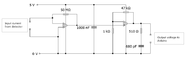
S2 Circuit Diagrams
S2.1 Output Circuit
The output circuit was required to change a V input to a A to A output current. Initially a buffer was used to ensure no current was drawn from the Arduino. The signal then passed through an RC filter to remove the D.C. offset. A potential divider was used to scale the voltage to the correct range followed by a series of amplifiers to scale the voltage to the right current and ensure the current was being drawn from an external power supply (Figure S1).
S2.2 Input Circuit
The input current from the detector was between 0 and 1 nA and needed to be converted to a voltage between 0 and 5 V. The circuit designed for this (Figure S2) uses an amplifier to convert the incoming current into a voltage followed by another amplifier to provide the correct magnitude. As the signal is only a very small current, it is susceptible to background noise. The cable from the detector was soldered directly onto the leg of the first amplifier to reduce the distance over which noise could be picked up and the whole circuit was placed as close as possible to the detector output.
The fixed gain of the circuit in Figure S2 and the limited resolution of the ADC in the Arduino limits the range over which the circuit is useful. It is sufficient to demonstrate the effectiveness of the method but would require a more sophisticated circuit to cover a dynamic range of 4 orders of magnitude observed in a typical experiment.
S3 Numerical Control System and Models in Simulink
The Simulink models used for the numerical models and hardware implementation are given in the figures below. Figure S3 shows the polarisation control system used in both the numerical models and the real life implementation. Included within this system are the lock-in amplifier subsystem shown in Figure S4 and the polarisation calculator shown in Figure S5. In the numerical model the detector current input came from the output of the machine model given in Figure S6 and the phase coil current output is used as the input to the machine model.
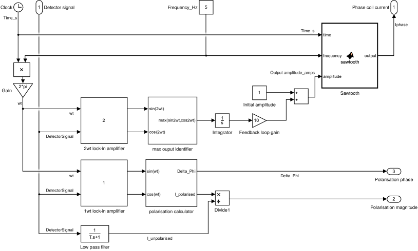
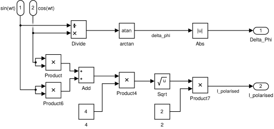
The polarisation calculator (Figure S5) uses the dependence of the detector count rate upon the phase coil current according to Equation 3 as introduced in the main text. (3) can be expanded to highlight the separation of the real and imaginary parts of the polarisation
| (S7) |
where and are the amplitudes of the real and imaginary part of the polarisation, respectively. The magnitude of the polarisation and the phase are then obtained via
| (S8) |
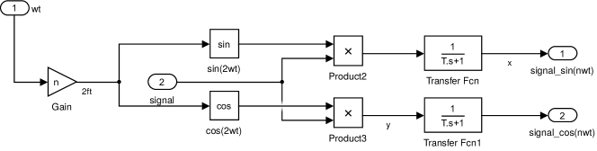
S3.1 Lock-In Amplifier
The concept of lock-in detection can be found in many textbooks. In this work a lock-in amplifier (Figure S4) is designed to extract one frequency component from a signal. To do this it multiplies the original signal with a sine wave of the frequency that one wants to extract. In Fourier space, this can be thought of as a convolution of the original signal with a pair of delta functions, one at the original frequency and one at minus the original frequency. It has the effect of moving the component of the original signal at the desired frequency to a constant component. A low pass filter of the form is then used so that only the D.C. part of this new signal remains, providing as an output the amplitude of the component oscillating at the desired frequency. To get the amplitude correct, a lock-in amplifier using a cosine wave is also used and the results of both are added in quadrature to account for any phase differences.