TTP18-006
Three-loop massive form factors: complete light-fermion corrections for the vector current

Abstract

We compute the three-loop QCD corrections to the massive quark-anti-quark-photon form factors $F_{1}$ and $F_{2}$ involving a closed loop of massless fermions. This subset is gauge invariant and contains both planar and non-planar contributions. We perform the reduction using FIRE and compute the master integrals with the help of differential equations. Our analytic results can be expressed in terms of Goncharov polylogarithms. We provide analytic results for all master integrals which are not present in the large-$N_{c}$ calculation considered in Refs. [1, 2].

1 Introduction

In the absence of striking experimental signals which hint to physics beyond the Standard Model it is of utmost importance to increase the precision of the theoretical predictions. A subsequent detailed comparison to precise measurements will help to uncover deviations and will provide hints for the construction of beyond-the-Standard-Model theories.

Quark and gluon form factors play a special role in the context of precision calculations. On the one hand they are sufficiently simple which allows to compute them to high order in perturbation theory. On the other hand they enter as building blocks into a variety of physical cross sections and decay rates, most prominently into Higgs boson production and decay, the Drell Yan production of leptons and the production of massive quarks. Form factors also constitute an ideal playground to study the infrared properties of a quantum field theory, in particular of QCD. As far as massless form factors are concerned the state-of-the-art is four loops where different groups have contributed to partial results [3, 4, 5, 6, 7, 8]. Massive quark form factors are known to two loops [9] including ${\cal O}(\epsilon)$ [10, 2] and ${\cal O}(\epsilon^{2})$ terms [11, 12]. Three-loop corrections in the large-$N_{c}$ limit for the vector current form factor have been computed in Ref. [2]. In this paper we extend these considerations and compute the complete contributions (i.e. all colour factors) from the diagrams involving a closed massless quark loop. This well-defined and gauge invariant subset contains for the first time non-planar contributions which we study in detail. Furthermore, new planar master integrals have to be evaluated which are not present in the large-$N_{c}$ result. As a by-product of our calculation we obtain the two-loop form factor including order $\epsilon^{2}$ terms. We do not consider singlet diagrams where the external photon couples to a closed massless quark loop which is connected via gluons to the final-state massive quarks. Such diagrams form again a separate gauge invariant subset which requires the computation of different integral families. Let us mention that all-order corrections to the massive form factor in the large-$\beta_{0}$ limit have been considered in Ref. [13].

The remainder of the paper is structured as follows: In the next Section we introduce the notation and discuss the ultraviolet and infrared divergences. One- and two-loop results are presented in Section 3. The three-loop calculation is described in Section 4, in particular the calculation of the master integrals. Section 5 contains a discussion of the three-loop form factor. We provide both numerical results and analytic expressions in various kinematical limits. In Section 6 we summarize our results and comment on the perspective for the full result.

2 Notation, renormalization and infrared structure

Let us define the form factors we are going to consider. Starting point is the photon-quark-anti-quark vertex which we introduce as

$$V^{\mu,ij}(q_{1},q_{2}) = \delta^{ij}\,\bar{u}(q_{1})\Gamma^{\mu}(q_{1},q_{2})v(q_{2})\,,$$ (1)

where $i$ and $j$ are (fundamental) colour indices and $\bar{u}(q_{1})$ and $v(q_{2})$ are the spinors of the quark and anti-quark, respectively, with incoming momentum $q_{1}$ and outgoing momentum $q_{2}$. The external quarks are on-shell, i.e., we have $q_{1}^{2}=q_{2}^{2}=m^{2}$. The form factors are defined as prefactors of the Lorentz decomposition of the vertex function $\Gamma^{\mu}(q_{1},q_{2})$ which is introduced as

$$\Gamma^{\mu}(q_{1},q_{2}) = Q_{q}\left[F_{1}(q^{2})\gamma^{\mu}-\frac{i}{2m}F_{2}(q^{2})\sigma^{\mu\nu}q_{\nu}\right]\,,$$ (2)

with $q=q_{1}-q_{2}$ being the outgoing momentum of the photon and $\sigma^{\mu\nu}=i[\gamma^{\mu},\gamma^{\nu}]/2$. $Q_{q}$ is the charge of the considered quark. For on-shell renormalized form factors we have $F_{1}(0)=1$ and $F_{2}(0)=(g-2)/2$ where $g$ is the gyromagnetic ratio of the quark (or lepton in the case of QED). For later convenience we define the perturbative expansion of $F_{1}$ and $F_{2}$ as

$$F_{i}=\sum_{n\geq 0}F_{i}^{(n)}\left(\frac{\alpha_{s}(\mu)}{4\pi}\right)^{n}\,,$$ (3)

with $F_{1}^{(0)}=1$ and $F_{2}^{(0)}=0$.

To obtain the renormalized form factors we use the $\overline{\rm MS}$ scheme for the strong coupling constant and the on-shell scheme for the heavy quark mass and wave function of the external quarks. In all cases the counterterm contributions are simply obtained by re-scaling the bare parameters with the corresponding renormalization constants, $Z_{\alpha_{s}}$, $Z_{m}^{\rm OS}$ and $Z_{2}^{\rm OS}$. The latter is needed to three loops whereas two-loop corrections for $Z_{\alpha_{s}}$ and $Z_{m}^{\rm OS}$ are sufficient to obtain renormalized three-loop results for $F_{1}$ and $F_{2}$. Note that higher order $\epsilon$ coefficients are needed for the on-shell renormalization constants since the one- and two-loop form factors develop $1/\epsilon$ and $1/\epsilon^{2}$ poles, respectively.

After renormalization of the ultraviolet divergences the form factors still contain infrared poles which are connected to the cusp anomalous dimension, $\Gamma_{\rm cusp}$ [14, 15, 16]. We adapt the notation from Ref. [2] and write

$$F=ZF^{f}\,,$$ (4)

where the factor $Z$, which is defined in the $\overline{\rm MS}$ scheme and thus only contains poles in $\epsilon$, absorbs the infrared divergences and $F^{f}$ is finite. The coefficients of the poles of $Z$ are determined by the QCD beta function and $\Gamma_{\rm cusp}$. In fact, the $1/\epsilon^{1}$ pole of the $\alpha_{s}^{n}$ term of $Z$ is proportional to the $n$-loop correction to $\Gamma_{\rm cusp}$ (see, e.g., Ref. [2].)

A dedicated calculation of $\Gamma_{\rm cusp}$ to three loops has been performed in Refs. [14, 16, 17, 18]. An independent cross check of the large-$N_{c}$ result has been provided in Ref. [2]. In this work we reproduce all $n_{l}$ terms at three-loop order by extracting $\Gamma_{\rm cusp}$ from the pole part of the form factors.

For the practical computation of the master integrals, for the discussion of the various kinematic limits and also for the numerical evaluation it is convenient to introduce the dimensionless variable

$$\frac{q^{2}}{m^{2}} = -\frac{(1-x)^{2}}{x}\,,$$ (5)

which maps the complex $q^{2}/m^{2}$ plane into the unit circle. The low-energy ($q^{2}\to 0$), high-energy ($q^{2}\to\infty$) and threshold ($q^{2}\to 4m^{2}$) limits correspond to $x\to 1$, $x\to 0$ and $x\to-1$, respectively. Furthermore, as can be seen in Fig. 1, the interval $q^{2}<0$ is mapped to $x\in(0,1)$ and $q^{2}\in[0,4m^{2}]$ to the upper semi-circle. For these values of $x$ the form factors have to be real-valued since the corresponding Feynman diagrams do not have cuts. This is different for the region $q^{2}>4m^{2}$, which corresponds to $x\in(-1,0)$, where the form factors are complex-valued.

For the threshold limit it is also convenient to introduce the velocity of the produced quarks

$$\beta = \sqrt{1-\frac{4m^{2}}{s}}\,,$$ (6)

which is related to $x$ via

$$x = \frac{2\beta}{1+\beta}-1\,.$$ (7)

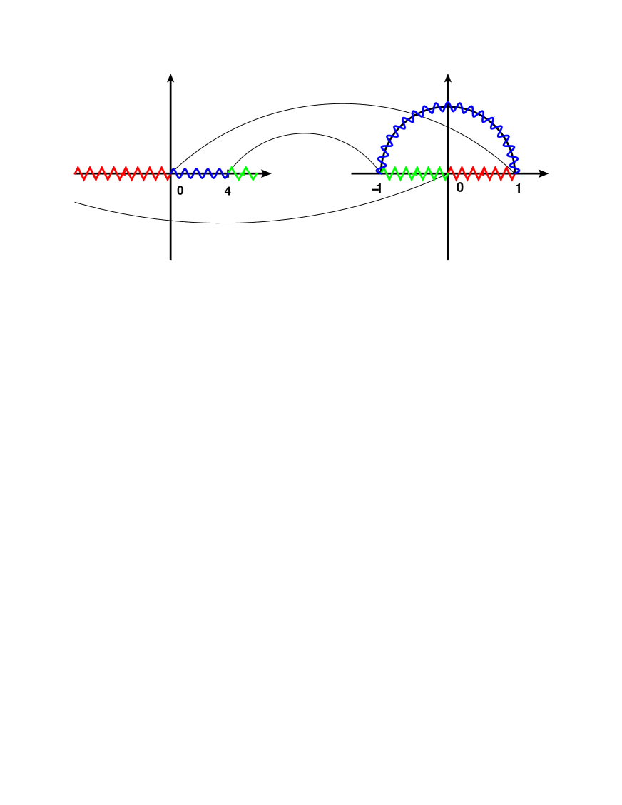
Figure 1: Illustration of the variable transformation between $q^{2}/m^{2}$ and $x$ as given in Eq. (5). The left graph represents the $q^{2}/m^{2}$ plane and on right the complex $x$ plane is shown. The straight lines indicate the mapping for special values of $q^{2}/m^{2}$ and $x$.

3 One- and two-loop form factors

Figure 2: Sample diagrams contributing to $F_{1}$ and $F_{2}$ at one and two loops. Solid, curly and wavy lines represent quarks, gluons and photons, respectively.

Let us in the following briefly outline the main steps of the two-loop calculation. Sample Feynman diagrams contributing to $F_{1}$ and $F_{2}$ can be found in Fig. 2. After generating the amplitudes we find it convenient to define one integral family at one and four integral families at two loops. We use FIRE [19] in combination with LiteRed [20, 21] for the reduction to master integrals within each family. After minimization we arrive at two and 17 master integrals at one- and two-loop order, respectively. For convenience we show the two one-loop and one two-loop master integrals explicitly in Fig. 3(a), (b) and (c). The remaining 16 two-loop integrals are obtained from  3(d) by reducing lines or adding dots according to

$$G(0,0,0,1,0,1,0),\,\,G(0,0,0,1,1,1,0),\,\,G(0,1,0,1,1,0,0),\,\,$$

$$G(0,1,0,1,2,0,0),\,\,G(0,1,1,0,0,1,0),\,\,G(0,1,1,0,1,1,0),\,\,$$

$$G(0,1,1,1,1,0,0),\,\,G(0,1,1,1,1,1,0),\,\,G(0,1,1,1,1,2,0),\,\,$$

$$G(1,0,0,1,0,1,0),\,\,G(1,0,0,1,1,1,0),\,\,G(1,0,0,1,1,2,0),\,\,$$

$$G(1,0,1,1,0,1,0),\,\,G(1,0,1,1,0,2,0),\,\,G(1,1,1,1,1,1,0),\,\,$$

$$G(1,1,1,1,1,2,0)\,.$$ (8)

In the large-$N_{c}$ limit only ten master integrals are needed at two loops.

(a)	(b)	(c)	(d)

Figure 3: The two one-loop master integrals are shown in (a) and (b). One of the 17 master two-loop integrals is shown in (c) and the remaining 16 master integrals are obtained from (d) as described in the text. Solid and dashed internal lines correspond to massive and massless scalar propagators. Thin external lines are on the mass shell and thick external lines carry the (off-shell) momentum $q$.

We evaluate all one- and two-loop master integrals analytically and expand in $\epsilon$ up to the order needed for the $\epsilon^{4}$ and $\epsilon^{2}$ terms of the one- and two-loop form factors, respectively. Our results are expressed in terms of Goncharov polylogarithms (GPLs) [22] with letters $-1,0$ and $+1$. We compared the ultraviolet-renormalized two-loop form factors to Ref. [10] and find agreement including order $\epsilon^{1}$ up to the discrepancy in $F_{1}$ already discussed in Section 4.4 of Ref. [2], see also Ref. [12] where agreement with our result is found. The order $\epsilon^{2}$ terms of $F_{1}$ and $F_{2}$ have recently been published in Ref. [12]; our results agree with theirs. Note that the large-$N_{c}$ limit of our result for $F_{1}$ has already been published in Ref. [11]. In this paper the $\epsilon^{2}$ terms have been used to derive higher-loop corrections with the help of renormalization group techniques. Apart from that, the $\epsilon^{2}$ terms also enter a future four-loop calculation of the massive form factors.

4 Three-loop form factor

(a)	(b)	(c)	(d)	(e)

Figure 4: Sample diagrams contributing to $F_{1}$ and $F_{2}$ at three-loop order. Solid, curly and wavy lines represent quarks, gluons and photons, respectively. In our calculation we only consider contributions with at least one closed massless quark loop.

In the following we concentrate on the contributions to $F_{1}$ and $F_{2}$ which contain at least one closed massless quark loop. Altogether there are 42 such vertex diagrams, 41 of them contain exactly one closed massless fermion loop and there is one diagram with two such closed loops. Sample Feynman diagrams contribution at three-loop order to the photon quark vertex are shown in Fig. 4.

Note that some of the contributing planar diagrams are already present in the large-$N_{c}$ limit [2] (see, e.g., Fig. 4(a)). However, other planar diagrams do not contribute to the leading $N_{c}$ term and thus the corresponding integral families have not been studied in Ref. [1]. For example, the amplitude of Fig. 4(b) is proportional to $C_{F}-C_{A}/2=1/(2N_{c})$. Furthermore, there are non-planar contributions (cf. Fig. 4(d)); all of them are sub-leading in the colour factor and are treated for the first time in this paper.

For the three-loop calculation we define ten integral families which are implemented in FIRE and LiteRed. Six of them can be taken over from the large-$N_{c}$ calculation [1, 2] and four are new. Three of the new families are planar and one is non-planar, see Fig. 5.

1051	1104	1136	1147

Figure 5: New three-loop integral families needed for the fermionic contributions to the three-loop vertex corrections. Solid and dashed lines represent massive and massless lines, respectively. Thin external lines are on the mass shell and thick external lines carry the off-shell momentum $q$. For convenience we keep our internal numeration of the integral families, which is shown below the Feynman diagrams.

To obtain results for the form factors we proceed as follows:

• We generate the amplitude for each diagram using qgraf [23] and transform the output to FORM [24] notation using q2e and exp [25, 26]. The latter is also used to identify for each diagram the corresponding family and to perform the mapping of the integration momenta.

• In a next step FORM is used to evaluate the Dirac algebra. We apply the projectors to $F_{1}$ and $F_{2}$, perform the traces and decompose the scalar products, which appear in the numerator, to factors, which are present in the definition of the corresponding integral family. At this point each integral can be represented as a function which has the powers of the individual propagator factors as arguments. The list of integrals serves as input for FIRE [19]. Note that we perform the calculation for general QCD gauge parameter $\xi$. $F_{1}$ and $F_{2}$ have to be independent of $\xi$ which serves as a welcome check for our calculation.

• We use FIRE [19] in combination with LiteRed [20, 21] to generate integral tables for the ten families. For the non-planar family, which is among the most complicated ones, this takes of the order of a week CPU time on a computer with about 100 GB RAM.

• Afterwards we minimize the set of the master integrals with the help of tsort, which is part of the latest FIRE version [19] (implemented in the command FindRules). It is based on ideas presented in Ref. [27], to obtain relations between primary master integrals, and to arrive at a minimal set. Next we derive a system of differential equations for the master integrals using LiteRed. We use FIRE to reduce integrals appearing on the right-hand side of the equations.

• In a next step we transform the system to $\epsilon$-form following the algorithm described in Ref. [28].

• Our final result can be expressed in terms of GPLs with letters $-1,0$ and $+1$, which is equivalent to Harmonic Polylogarithms (HPLs) [29]. Still we prefer to work with results in terms of GPLs, in particular, when taking various limits, because we use the same setup as in Refs. [1, 2]. Furthermore, in the calculation of the non-fermionic contributions to the massive form factor it will not be possible to express the result in terms of HPLs (see also Refs. [1, 2]).

• We consider the limit $q^{2}\to 0$ to fix the boundary conditions. In this limit the vertex integrals become two-point on-shell integrals which are well-studied at three-loop order. We take the results from Ref. [30].

Results for all 89 planar master integrals entering the large-$N_{c}$ expressions for the form factors have been discussed in Ref. [1] and explicit results have been presented. In an ancillary file to this paper [31] we present results for all master integrals entering our results, which are not considered in Ref. [1]. After minimizing the master integrals of the four new families we observe that all integrals from family 1136 can be mapped either to 1104 or 1147 or to the planar families studied in Ref. [1] and we have to compute 15 new three-loop master integrals from three families to obtain the results presented in this paper. They are given by

$$G_{1051}(0,0,1,0,1,1,1,2,1,0,0,0),\,\,G_{1051}(1,0,0,1,2,0,1,1,0,0,0,0),\,\,$$

$$G_{1051}(1,0,1,1,1,1,1,1,0,0,0,0),\,\,G_{1051}(1,0,1,1,1,1,1,2,0,0,0,0),\,\,$$

$$G_{1104}(1,0,0,0,1,1,1,0,1,0,0,0),\,\,G_{1104}(1,0,0,0,1,1,1,0,2,0,0,0),\,\,$$

$$G_{1104}(1,0,0,0,1,1,2,0,1,0,0,0),\,\,G_{1104}(1,0,1,0,1,1,1,0,1,0,0,0),\,\,$$

$$G_{1104}(1,0,1,0,1,1,1,0,2,0,0,0),\,\,G_{1147}(0,1,0,0,1,1,1,1,0,0,0,0),\,\,$$

$$G_{1147}(1,0,0,1,1,1,1,1,0,0,0,0),\,\,G_{1147}(1,0,0,1,1,1,1,2,0,0,0,0),\,\,$$

$$G_{1147}(1,0,0,1,1,2,1,1,0,0,0,0),\,\,G_{1147}(1,1,0,0,1,1,1,1,0,0,0,0),\,\,$$

$$G_{1147}(1,1,0,0,1,1,1,2,0,0,0,0)\,,$$ (9)

where the order of the indices corresponds to the line numbers introduced in Fig. 5 and thus it is straightforward to construct the integrands. Note that the last three indices represent irreducible numerators. Since they are zero for all our integrals their precise definition is irrelevant and we refrain from specifying them. For all integrals in Eq. (9) we provide explicit results in [31]. We assume an integration measure $e^{\epsilon\gamma_{E}}{\rm d}^{D}k/(i\pi)^{D/2}$ with $D=4-2\epsilon$ and scalar propagators of the form $1/(m^{2}-k^{2})$ or $1/(-k^{2})$. Note that the above list only contains two non-planar integrals, $G_{1051}(1,0,1,1,1,1,1,1,0,0,0,0)$ and $G_{1051}(1,0,1,1,1,1,1,2,0,0,0,0)$.

5 Analytical and numerical results

In this section we discuss the results for the form factors $F_{1}$ and $F_{2}$. The analytic results expressed in terms of GPLs are quite long and we only present them in electronic form [31]. As already mentioned above, they do not constitute physical results and in general still contain poles in $\epsilon$. Thus, we exemplify the numerical results by considering the $\epsilon$-independent Taylor coefficient.

We start with discussing analytic results in the low- and high-energy and the threshold limit. The corresponding analytic expressions are also contained in an ancillary file to this paper [31]. They are obtained by expanding the Goncharov polylogarithms of the exact result in the relevant limits. Afterwards we demonstrate in Subsection 5.4 that a simple numerical evaluation of $F_{1}$ and $F_{2}$ is possible.

5.1 Form factors in the static limit

In the static limit the form factors are infrared finite and thus $F_{1}$ and $F_{2}$ do not contain poles in $\epsilon$. In the on-shell scheme $F_{1}(q^{2}=0)=1$ and $F_{2}(q^{2}=0)$ is related to the quark anomalous magnetic moment which we use as a cross check. Note that we use the limit $q^{2}\to 0$ to fix the boundary conditions for the master integrals (see discussion in Section 4). However, this only requires as input scalar three-loop two-point on-shell integrals (see Ref. [30]) and thus the limit of the final analytic expression for the form factor can still be used as cross check. In fact, our explicit calculation shows that $F_{1}(q^{2}=0)=1$ and $F_{2}(q^{2}=0)$ agrees with the dedicated three-loop calculation from Ref. [32].

We computed $F_{1}$ and $F_{2}$ up to order $(1-x)^{6}$ and refer to the ancillary file for the complete expressions. In the following we present results for $F_{1}$ and $F_{2}$ up to ${\cal O}(\phi^{2})$ including the constant term in $\epsilon$. To obtain a manifest expansion $q^{2}\to 0$ for $q^{2}>0$ we use the variable $x=e^{i\phi}$ and display terms up to order $\phi^{2}$. For $\mu^{2}=m^{2}$ we obtain the following results for $F_{1}$

$$F_{1}^{(1)} = \phi^{2}C_{F}\Bigg{[}-\frac{2}{3\epsilon}-\frac{1}{2}\Bigg{]}+{\cal O}(\epsilon)\,,$$

$$F_{1}^{(2)} = \phi^{2}\Bigg{\{}C_{F}^{2}\Bigg{[}-12\zeta(3)-\frac{47}{36}-\frac{175\pi^{2}}{54}+8\pi^{2}l_{2}\Bigg{]}$$

$$\mbox{}+C_{A}C_{F}\Bigg{[}\frac{11}{9\epsilon^{2}}+\frac{\frac{2\pi^{2}}{9}-\frac{94}{27}}{\epsilon}+\frac{26\zeta(3)}{3}+\frac{155\pi^{2}}{108}-\frac{2579}{324}-4\pi^{2}l_{2}\Bigg{]}$$

$$\mbox{}+C_{F}T_{F}n_{l}\Bigg{[}-\frac{4}{9\epsilon^{2}}+\frac{20}{27\epsilon}+\frac{8\pi^{2}}{27}+\frac{283}{81}\Bigg{]}+C_{F}T_{F}n_{h}\Bigg{[}\frac{3\pi^{2}}{2}-\frac{1099}{81}\Bigg{]}\Bigg{\}}$$

$$\mbox{}+{\cal O}(\epsilon)\,,$$

$$F_{1}^{(3)}\Big{|}_{n_{l}} = \phi^{2}\Bigg{\{}C_{F}^{2}T_{F}n_{l}\Bigg{[}-\frac{8}{9\epsilon^{2}}+\frac{\frac{110}{27}-\frac{32\zeta(3)}{9}}{\epsilon}+\frac{512a_{4}}{3}+\frac{64l_{2}^{4}}{9}+\frac{128\pi^{2}l_{2}^{2}}{9}$$ (10)

$$\mbox{}-\frac{1768\pi^{2}l_{2}}{27}+\frac{1100\zeta(3)}{9}-\frac{448\pi^{4}}{135}+\frac{9838\pi^{2}}{243}-\frac{3107}{162}\Bigg{]}$$

$$\mbox{}+C_{A}C_{F}T_{F}n_{l}\Bigg{[}\frac{176}{81\epsilon^{3}}+\frac{\frac{16\pi^{2}}{81}-\frac{1552}{243}}{\epsilon^{2}}+\frac{\frac{112\zeta(3)}{27}-\frac{160\pi^{2}}{243}+\frac{1556}{243}}{\epsilon}-\frac{256a_{4}}{3}$$

$$\mbox{}-\frac{32l_{2}^{4}}{9}-\frac{64\pi^{2}l_{2}^{2}}{9}+\frac{884\pi^{2}l_{2}}{27}-\frac{1622\zeta(3)}{27}+\frac{352\pi^{4}}{405}-\frac{5237\pi^{2}}{729}+\frac{260644}{2187}\Bigg{]}$$

$$\mbox{}+C_{F}T_{F}^{2}n_{l}^{2}\Bigg{[}-\frac{32}{81\epsilon^{3}}+\frac{160}{243\epsilon^{2}}+\frac{32}{243\epsilon}-\frac{448\zeta(3)}{81}-\frac{464\pi^{2}}{243}-\frac{29524}{2187}\Bigg{]}$$

$$\mbox{}+C_{F}T_{F}^{2}n_{h}n_{l}\Bigg{[}\frac{8\pi^{2}}{81\epsilon}-\frac{8\pi^{2}l_{2}}{3}+\frac{724\zeta(3)}{81}-\frac{892\pi^{2}}{243}+\frac{10088}{243}\Bigg{]}\Bigg{\}}+{\cal O}(\epsilon)\,,$$

where $l_{2}=\log(2)$ and $a_{4}=\mbox{Li}_{4}(1/2)$. For $F_{2}$ we have

$$F_{2}^{(1)} = 2C_{F}+\phi^{2}\frac{C_{F}}{3}+{\cal O}(\epsilon)\,,$$

$$F_{2}^{(2)} = C_{F}^{2}\Bigg{[}-8\pi^{2}l_{2}+12\zeta(3)+\frac{20\pi^{2}}{3}-31\Bigg{]}+C_{A}C_{F}\Bigg{[}4\pi^{2}l_{2}-6\zeta(3)-2\pi^{2}+\frac{317}{9}\Bigg{]}$$

$$\mbox{}+C_{F}T_{F}n_{l}\Bigg{[}-\frac{100}{9}\Bigg{]}+C_{F}T_{F}n_{h}\Bigg{[}\frac{476}{9}-\frac{16\pi^{2}}{3}\Bigg{]}+\phi^{2}\Bigg{\{}C_{F}^{2}\Bigg{[}-\frac{4}{3\epsilon}-\frac{92\pi^{2}l_{2}}{15}$$

$$\mbox{}+\frac{46\zeta(3)}{5}+\frac{61\pi^{2}}{15}-\frac{77}{5}\Bigg{]}+C_{A}C_{F}\Bigg{[}\frac{46\pi^{2}l_{2}}{15}-\frac{23\zeta(3)}{5}-\frac{137\pi^{2}}{90}+\frac{1699}{270}\Bigg{]}$$

$$\mbox{}+C_{F}T_{F}n_{l}\Bigg{[}-\frac{62}{27}\Bigg{]}+C_{F}T_{F}n_{h}\Bigg{[}\frac{622}{27}-\frac{7\pi^{2}}{3}\Bigg{]}\Bigg{\}}+{\cal O}(\epsilon)\,,$$

$$F_{2}^{(3)}\Big{|}_{n_{l}} = C_{F}^{2}T_{F}n_{l}\Bigg{[}-\frac{512a_{4}}{3}-\frac{64l_{2}^{4}}{9}-\frac{128\pi^{2}l_{2}^{2}}{9}+\frac{320\pi^{2}l_{2}}{3}-192\zeta(3)+\frac{88\pi^{4}}{27}-\frac{2528\pi^{2}}{27}$$ (11)

$$\mbox{}+250\Bigg{]}+C_{A}C_{F}T_{F}n_{l}\Bigg{[}\frac{256a_{4}}{3}+\frac{32l_{2}^{4}}{9}+\frac{64\pi^{2}l_{2}^{2}}{9}-\frac{160\pi^{2}l_{2}}{3}+\frac{304\zeta(3)}{3}-\frac{44\pi^{4}}{27}$$

$$\mbox{}+\frac{616\pi^{2}}{27}-\frac{38576}{81}\Bigg{]}+C_{F}T_{F}^{2}n_{l}^{2}\Bigg{[}\frac{5072}{81}+\frac{64\pi^{2}}{27}\Bigg{]}+C_{F}T_{F}^{2}n_{h}n_{l}\Bigg{[}\frac{64\pi^{2}}{27}-\frac{1952}{81}\Bigg{]}$$

$$\mbox{}+\phi^{2}\Bigg{\{}C_{F}^{2}T_{F}n_{l}\Bigg{[}-\frac{5888a_{4}}{45}-\frac{8}{9\epsilon^{2}}+\frac{16}{3\epsilon}-\frac{736l_{2}^{4}}{135}-\frac{1472\pi^{2}l_{2}^{2}}{135}+\frac{8048\pi^{2}l_{2}}{135}$$

$$\mbox{}-\frac{664\zeta(3)}{5}+\frac{1012\pi^{4}}{405}-\frac{6092\pi^{2}}{135}+\frac{12653}{90}\Bigg{]}+C_{A}C_{F}T_{F}n_{l}\Bigg{[}\frac{2944a_{4}}{45}+\frac{368l_{2}^{4}}{135}$$

$$\mbox{}+\frac{736\pi^{2}l_{2}^{2}}{135}-\frac{4024\pi^{2}l_{2}}{135}+\frac{348\zeta(3)}{5}-\frac{506\pi^{4}}{405}+\frac{458\pi^{2}}{27}-\frac{26626}{243}\Bigg{]}$$

$$\mbox{}+C_{F}T_{F}^{2}n_{l}^{2}\Bigg{[}\frac{3736}{243}+\frac{32\pi^{2}}{81}\Bigg{]}+C_{F}T_{F}^{2}n_{h}n_{l}\Bigg{[}\frac{16\pi^{2}l_{2}}{9}-\frac{56\zeta(3)}{9}+\frac{40\pi^{2}}{9}$$

$$\mbox{}-\frac{11824}{243}\Bigg{]}\Bigg{\}}+{\cal O}(\epsilon)\,.$$

Note that starting from the next-to-leading expansion term of order $\phi^{2}$ both $F_{1}$ and $F_{2}$ are infrared divergent and develops poles in $\epsilon$.

5.2 Form factors at high energies

In the limit $x\to 0$ we compute terms up to ${\cal O}(x^{6})$ both for $F_{1}$ and $F_{2}$. To illustrate the structure of the analytic expressions we show the first two terms of order $x^{0}$ and $x^{1}$ for $F_{1}$ at three loops. After introducing the notation

$$F_{i}^{(n)} = \sum_{k\geq 0}f_{i,\rm lar}^{(n,k)}x^{k}\,.$$ (12)

we have

$$f_{1,\rm lar}^{(1,0)} = C_{F}\Bigg{[}\left(-\frac{2}{\epsilon}-3\right)l_{x}-\frac{2}{\epsilon}-l_{x}^{2}+\frac{\pi^{2}}{3}-4\Bigg{]}\,,$$

$$f_{1,\rm lar}^{(1,1)} = C_{F}\Bigg{[}2l_{x}-4\Bigg{]}\,,$$

$$f_{1,\rm lar}^{(2,0)} = C_{F}^{2}\Bigg{[}\left(\frac{2}{\epsilon^{2}}+\frac{8}{\epsilon}-\frac{2\pi^{2}}{3}+\frac{55}{2}\right)l_{x}^{2}+l_{x}\left(\frac{4}{\epsilon^{2}}+\frac{14-\frac{2\pi^{2}}{3}}{\epsilon}-32\zeta(3)+\frac{85}{2}\right)+\frac{2}{\epsilon^{2}}$$

$$\mbox{}+\left(\frac{2}{\epsilon}+\frac{20}{3}\right)l_{x}^{3}+\frac{8-\frac{2\pi^{2}}{3}}{\epsilon}+\frac{7l_{x}^{4}}{6}-44\zeta(3)-\frac{59\pi^{4}}{90}+\frac{13\pi^{2}}{2}+46-8\pi^{2}l_{2}\Bigg{]}$$

$$\mbox{}+C_{A}C_{F}\Bigg{[}l_{x}\left(\frac{11}{3\epsilon^{2}}+\frac{\frac{\pi^{2}}{3}-\frac{67}{9}}{\epsilon}+26\zeta(3)-\frac{11\pi^{2}}{9}-\frac{2545}{54}\right)$$

$$\mbox{}+\frac{11}{3\epsilon^{2}}+\frac{-2\zeta(3)-\frac{49}{9}+\frac{\pi^{2}}{3}}{\epsilon}-\frac{11l_{x}^{3}}{9}+\left(\frac{\pi^{2}}{3}-\frac{233}{18}\right)l_{x}^{2}$$

$$\mbox{}+\frac{134\zeta(3)}{3}-\frac{\pi^{4}}{60}-\frac{7\pi^{2}}{54}-\frac{1595}{27}+4\pi^{2}l_{2}\Bigg{]}$$

$$\mbox{}+C_{F}T_{F}n_{l}\Bigg{[}\left(-\frac{4}{3\epsilon^{2}}+\frac{20}{9\epsilon}+\frac{4\pi^{2}}{9}+\frac{418}{27}\right)l_{x}$$

$$\mbox{}-\frac{4}{3\epsilon^{2}}+\frac{20}{9\epsilon}+\frac{4l_{x}^{3}}{9}+\frac{38l_{x}^{2}}{9}-\frac{16\zeta(3)}{3}-\frac{14\pi^{2}}{27}+\frac{424}{27}\Bigg{]}$$

$$\mbox{}+C_{F}T_{F}n_{h}\Bigg{[}\frac{4l_{x}^{3}}{9}+\frac{38l_{x}^{2}}{9}+\left(\frac{530}{27}+\frac{2\pi^{2}}{3}\right)l_{x}-\frac{4\pi^{2}}{9}+\frac{1532}{27}\Bigg{]}\,,$$

$$f_{1,\rm lar}^{(2,1)} = C_{F}^{2}\Bigg{[}\left(-\frac{4}{\epsilon}+\frac{4\pi^{2}}{3}-37\right)l_{x}^{2}+l_{x}\left(\frac{4}{\epsilon}-48\zeta(3)+6\pi^{2}+13\right)$$

$$\mbox{}+\frac{8}{\epsilon}-\frac{l_{x}^{4}}{3}-\frac{28l_{x}^{3}}{3}-88\zeta(3)+\frac{32\pi^{4}}{45}-5\pi^{2}-22+48\pi^{2}l_{2}\Bigg{]}$$

$$\mbox{}+C_{A}C_{F}\Bigg{[}\frac{l_{x}^{4}}{6}+\frac{8l_{x}^{3}}{3}+\left(\frac{4\pi^{2}}{3}-\frac{25}{3}\right)l_{x}^{2}+l_{x}\left(-72\zeta(3)+\frac{341}{9}+\frac{22\pi^{2}}{3}\right)$$

$$\mbox{}-200\zeta(3)+\frac{7\pi^{4}}{9}+\frac{247\pi^{2}}{9}-\frac{904}{9}-24\pi^{2}l_{2}\Bigg{]}$$

$$\mbox{}+C_{F}T_{F}n_{l}\Bigg{[}-\frac{4l_{x}^{2}}{3}-\frac{148l_{x}}{9}+\frac{4\pi^{2}}{9}+\frac{200}{9}\Bigg{]}$$

$$\mbox{}+C_{F}T_{F}n_{h}\Bigg{[}-\frac{52l_{x}^{2}}{3}-\frac{436l_{x}}{9}-\frac{44\pi^{2}}{3}-\frac{784}{9}\Bigg{]}\,,$$

$$f_{1,\rm lar}^{(3,0)}\Big{|}_{n_{l}} = C_{F}^{2}T_{F}n_{l}\Bigg{[}\frac{8}{3\epsilon^{3}}+\left(\frac{4}{3\epsilon^{2}}-\frac{82}{9\epsilon}-\frac{29\pi^{2}}{27}-\frac{2032}{27}\right)l_{x}^{3}+\frac{-\frac{16}{9}-\frac{4\pi^{2}}{9}}{\epsilon^{2}}$$

$$\mbox{}+l_{x}^{2}\left(\frac{8}{3\epsilon^{3}}+\frac{8}{9\epsilon^{2}}+\frac{-\frac{962}{27}-\frac{10\pi^{2}}{9}}{\epsilon}+\frac{232\zeta(3)}{9}-\frac{50\pi^{2}}{9}-\frac{18817}{81}\right)$$

$$\mbox{}+l_{x}\left(\frac{16}{3\epsilon^{3}}+\frac{-\frac{20}{9}-\frac{4\pi^{2}}{9}}{\epsilon^{2}}+\frac{-\frac{16\zeta(3)}{3}-\frac{1198}{27}+\frac{2\pi^{2}}{9}}{\epsilon}+\frac{1976\zeta(3)}{9}+\frac{98\pi^{4}}{135}-\frac{341\pi^{2}}{27}\right.$$

$$\left.\mbox{}-\frac{18812}{81}\right)+\left(-\frac{4}{9\epsilon}-\frac{355}{27}\right)l_{x}^{4}+\frac{-\frac{16\zeta(3)}{3}-\frac{470}{27}+\frac{4\pi^{2}}{3}}{\epsilon}-l_{x}^{5}-\frac{512}{3}a_{4}$$

$$\mbox{}+40\zeta(5)-8\pi^{2}\zeta(3)+\frac{2752\zeta(3)}{9}+\frac{3058\pi^{4}}{405}-\frac{481\pi^{2}}{9}-\frac{2011}{81}-\frac{64l_{2}^{4}}{9}$$

$$\mbox{}-\frac{128}{9}\pi^{2}l_{2}^{2}+\frac{224}{9}\pi^{2}l_{2}\Bigg{]}$$

$$\mbox{}+C_{A}C_{F}T_{F}n_{l}\Bigg{[}\frac{176}{27\epsilon^{3}}+\frac{-\frac{16\zeta(3)}{9}-\frac{1192}{81}+\frac{8\pi^{2}}{27}}{\epsilon^{2}}+l_{x}\left(\frac{176}{27\epsilon^{3}}+\frac{\frac{8\pi^{2}}{27}-\frac{1336}{81}}{\epsilon^{2}}\right.$$

$$\left.\mbox{}+\frac{\frac{112\zeta(3)}{9}+\frac{836}{81}-\frac{80\pi^{2}}{81}}{\epsilon}-\frac{1448\zeta(3)}{9}-\frac{22\pi^{4}}{135}+\frac{5864\pi^{2}}{243}+\frac{309838}{729}\right)$$

$$\mbox{}+\frac{\frac{496\zeta(3)}{27}+\frac{356}{81}-\frac{80\pi^{2}}{81}}{\epsilon}+\frac{44l_{x}^{4}}{27}+\left(\frac{1948}{81}-\frac{8\pi^{2}}{27}\right)l_{x}^{3}+l_{x}^{2}\left(-16\zeta(3)+\frac{11752}{81}\right.$$

$$\left.\mbox{}+\frac{16\pi^{2}}{9}\right)+\frac{256}{3}a_{4}+\frac{596\zeta(5)}{3}+\frac{4\pi^{2}\zeta(3)}{9}-\frac{31120\zeta(3)}{81}-\frac{1822\pi^{4}}{405}$$

$$\mbox{}+\frac{1504\pi^{2}}{243}+\frac{259150}{729}+\frac{32l_{2}^{4}}{9}+\frac{64}{9}\pi^{2}l_{2}^{2}-\frac{112}{9}\pi^{2}l_{2}\Bigg{]}$$

$$\mbox{}+C_{F}T_{F}^{2}n_{l}^{2}\Bigg{[}-\frac{32}{27\epsilon^{3}}+\frac{160}{81\epsilon^{2}}+l_{x}\left(-\frac{32}{27\epsilon^{3}}+\frac{160}{81\epsilon^{2}}+\frac{32}{81\epsilon}-\frac{64\zeta(3)}{27}-\frac{304\pi^{2}}{81}\right.$$

$$\left.\mbox{}-\frac{39352}{729}\right)+\frac{32}{81\epsilon}-\frac{8l_{x}^{4}}{27}-\frac{304l_{x}^{3}}{81}+\left(-\frac{1624}{81}-\frac{16\pi^{2}}{27}\right)l_{x}^{2}+\frac{256\zeta(3)}{9}+\frac{232\pi^{4}}{405}$$

$$\mbox{}-\frac{488\pi^{2}}{243}-\frac{29344}{729}\Bigg{]}$$

$$\mbox{}+C_{F}T_{F}^{2}n_{h}n_{l}\Bigg{[}l_{x}\left(\frac{8\pi^{2}}{27\epsilon}-\frac{416\zeta(3)}{27}-8\pi^{2}-\frac{7408}{81}\right)+\frac{8\pi^{2}}{27\epsilon}-\frac{16l_{x}^{4}}{27}-\frac{608l_{x}^{3}}{81}$$

$$\mbox{}+\left(-\frac{3248}{81}-\frac{32\pi^{2}}{27}\right)l_{x}^{2}-\frac{416\zeta(3)}{9}-\frac{16\pi^{4}}{27}+\frac{776\pi^{2}}{243}-\frac{5072}{27}\Bigg{]}\,,$$

$${f_{1,\rm lar}^{(3,1)}\Big{|}_{n_{l}}} = C_{F}^{2}T_{F}n_{l}\Bigg{[}l_{x}^{2}\left(-\frac{8}{3\epsilon^{2}}+\frac{92}{3\epsilon}+\frac{16\zeta(3)}{3}-\frac{178\pi^{2}}{27}+\frac{3416}{9}\right)$$ (13)

$$\mbox{}+l_{x}\left(\frac{8}{3\epsilon^{2}}+\frac{-\frac{32}{3}-\frac{4\pi^{2}}{9}}{\epsilon}+\frac{224\zeta(3)}{3}+\frac{344\pi^{4}}{135}-\frac{2918\pi^{2}}{27}+\frac{790}{9}\right)$$

$$\mbox{}+\frac{16}{3\epsilon^{2}}+\left(\frac{4}{3\epsilon}-\frac{8\pi^{2}}{3}+\frac{3436}{27}\right)l_{x}^{3}+\frac{-40-\frac{4\pi^{2}}{9}}{\epsilon}+\frac{4l_{x}^{5}}{9}+\frac{352l_{x}^{4}}{27}+1024a_{4}$$

$$\mbox{}-\frac{1312\zeta(5)}{3}+\frac{64\pi^{2}\zeta(3)}{3}+\frac{4528\zeta(3)}{9}-\frac{524\pi^{4}}{405}+\frac{3400\pi^{2}}{27}-\frac{1676}{9}+\frac{128l_{2}^{4}}{3}$$

$$\mbox{}+\frac{256}{3}\pi^{2}l_{2}^{2}-\frac{1664}{3}\pi^{2}l_{2}\Bigg{]}$$

$$\mbox{}+C_{A}C_{F}T_{F}n_{l}\Bigg{[}-\frac{2l_{x}^{5}}{9}-\frac{116l_{x}^{4}}{27}+\left(-\frac{160}{27}-\frac{4\pi^{2}}{3}\right)l_{x}^{3}+l_{x}^{2}\left(\frac{232\zeta(3)}{3}+\frac{104}{27}\right.$$

$$\left.\mbox{}-\frac{520\pi^{2}}{27}\right)+l_{x}\left(560\zeta(3)-\frac{34664}{81}-\frac{788\pi^{2}}{9}+\frac{236\pi^{4}}{135}\right)-512a_{4}$$

$$\mbox{}-\frac{1840\zeta(5)}{3}-\frac{32\pi^{2}\zeta(3)}{3}+\frac{14440\zeta(3)}{9}+\frac{868\pi^{4}}{405}-\frac{16988\pi^{2}}{81}+\frac{97384}{81}$$

$$\mbox{}-\frac{64l_{2}^{4}}{3}-\frac{128}{3}\pi^{2}l_{2}^{2}+\frac{832}{3}\pi^{2}l_{2}\Bigg{]}$$

$$\mbox{}+C_{F}T_{F}^{2}n_{l}^{2}\Bigg{[}\frac{32l_{x}^{3}}{27}+\frac{592l_{x}^{2}}{27}+\left(\frac{8720}{81}+\frac{32\pi^{2}}{27}\right)l_{x}-\frac{128\zeta(3)}{9}-\frac{976\pi^{2}}{81}-\frac{11296}{81}\Bigg{]}$$

$$\mbox{}+C_{F}T_{F}^{2}n_{h}n_{l}\Bigg{[}\frac{448l_{x}^{3}}{27}+\frac{3104l_{x}^{2}}{27}+\left(\frac{15136}{81}+\frac{448\pi^{2}}{27}\right)l_{x}+\frac{1664\zeta(3)}{9}$$

$$\mbox{}+\frac{5696\pi^{2}}{81}-\frac{5408}{81}\Bigg{]}\,,$$

where $l_{x}=\log(x)$. It is interesting to note that at three-loop order $l_{x}$ may in principle appear up to sixth power. However, for the $n_{l}$ terms at most $l_{x}^{5}$ terms are present. In the case of $f_{1,\rm lar}^{(3,0)}$ the $l_{x}^{6}$ term comes with the colour factor $C_{F}^{3}$ which is known since long [33, 34]. In Ref. [35, 36, 37] it has been shown that the $l_{x}^{6}$ term in the power-suppressed contribution $f_{1,\rm lar}^{(3,1)}$ comes together with colour structures $C_{F}-C_{A}/2$ in the $n_{l}$-independent term. Explicit results for power-suppressed terms are given in Ref. [36].

For $F_{2}$ we have $f_{2,\rm lar}^{(n,0)}=0$ (for $n=1,2$ and $3$) and

$$f_{2,\rm lar}^{(1,1)} = -4C_{F}l_{x}\,,$$

$$f_{2,\rm lar}^{(2,1)} = C_{F}^{2}\Bigg{[}\left(\frac{8}{\epsilon}+34\right)l_{x}^{2}+\left(\frac{8}{\epsilon}-8\pi^{2}+62\right)l_{x}-32\pi^{2}l_{2}+8l_{x}^{3}+16\zeta(3)+10\pi^{2}\Bigg{]}$$

$$\mbox{}+C_{A}C_{F}\Bigg{[}16\pi^{2}l_{2}+\frac{2l_{x}^{2}}{3}-\frac{346l_{x}}{9}+80\zeta(3)-\frac{122\pi^{2}}{9}+12\Bigg{]}$$

$$\mbox{}+C_{F}T_{F}n_{l}\Bigg{[}\frac{8l_{x}^{2}}{3}+\frac{200l_{x}}{9}-\frac{8\pi^{2}}{9}\Bigg{]}+C_{F}T_{F}n_{h}\Bigg{[}\frac{8l_{x}^{2}}{3}+\frac{200l_{x}}{9}-\frac{8\pi^{2}}{3}+\frac{272}{3}\Bigg{]}\,,$$

$$f_{2,\rm lar}^{(3,1)} = C_{F}^{2}T_{F}n_{l}\Bigg{[}-\frac{2048a_{4}}{3}+\left(\frac{16}{3\epsilon^{2}}-\frac{104}{3\epsilon}-\frac{28\pi^{2}}{9}-\frac{2936}{9}\right)l_{x}^{2}+l_{x}\left(\frac{16}{3\epsilon^{2}}\right.$$ (14)

$$\left.\mbox{}+\frac{\frac{8\pi^{2}}{9}-32}{\epsilon}+\frac{416\zeta(3)}{3}+\frac{1588\pi^{2}}{27}-\frac{4172}{9}\right)+\left(-\frac{8}{3\epsilon}-\frac{832}{9}\right)l_{x}^{3}+\frac{8\pi^{2}}{9\epsilon}$$

$$\mbox{}-\frac{256l_{2}^{4}}{9}-\frac{512\pi^{2}l_{2}^{2}}{9}+\frac{2816\pi^{2}l_{2}}{9}-\frac{80l_{x}^{4}}{9}-\frac{3328\zeta(3)}{9}+\frac{656\pi^{4}}{135}-\frac{2720\pi^{2}}{27}+\frac{16}{3}\Bigg{]}$$

$$\mbox{}+C_{A}C_{F}T_{F}n_{l}\Bigg{[}\frac{1024a_{4}}{3}+\frac{128l_{2}^{4}}{9}+\frac{256\pi^{2}l_{2}^{2}}{9}-\frac{1408\pi^{2}l_{2}}{9}+\frac{64l_{x}^{3}}{27}+\left(\frac{1256}{27}\right.$$

$$\left.\mbox{}+\frac{40\pi^{2}}{9}\right)l_{x}^{2}+l_{x}\left(-\frac{512\zeta(3)}{3}+\frac{1168\pi^{2}}{27}+\frac{44320}{81}\right)-\frac{2192\zeta(3)}{3}-\frac{8\pi^{4}}{3}$$

$$\mbox{}+\frac{8080\pi^{2}}{81}-\frac{496}{3}\Bigg{]}+C_{F}T_{F}^{2}n_{l}^{2}\Bigg{[}-\frac{64l_{x}^{3}}{27}-\frac{800l_{x}^{2}}{27}+\left(-\frac{10144}{81}-\frac{64\pi^{2}}{27}\right)l_{x}$$

$$\mbox{}+\frac{256\zeta(3)}{9}+\frac{800\pi^{2}}{81}\Bigg{]}+C_{F}T_{F}^{2}n_{h}n_{l}\Bigg{[}-\frac{128l_{x}^{3}}{27}-\frac{1600l_{x}^{2}}{27}$$

$$\mbox{}+\left(-\frac{20288}{81}-\frac{128\pi^{2}}{27}\right)l_{x}-\frac{256\zeta(3)}{9}-\frac{3712\pi^{2}}{81}-\frac{2240}{27}\Bigg{]}\,.$$

5.3 Form factors and threshold cross section

In the threshold limit ($q^{2}\to 4m^{2}$ or $x\to-1$) the form factors $F_{1}$ and $F_{2}$ can be used to obtain the physical cross section for $e^{+}e^{-}\to\mbox{hadrons}$ since they constitute the virtual corrections and the real corrections are suppressed by a relative factor $\beta^{3}$. This means that we can predict $\sigma(e^{+}e^{-}\to Q\bar{Q})$ including terms of order $\beta^{2-n}$ at $n$-loop order. Since for the three-loop $n_{l}$ contribution the $\beta^{0}$ terms computed from $F_{1}$ and $F_{2}$ are finite, we also show them below.

For convenience we repeat the formula which can be used to compute the cross section from the form factors (see also Ref. [2]) which reads

$$\sigma(e^{+}e^{-}\to Q\bar{Q}) = \sigma_{0}\beta\left[|F_{1}+F_{2}|^{2}+\frac{|(1-\beta^{2})F_{1}+F_{2}|^{2}}{2(1-\beta^{2})}\right]$$ (15)

$$= \sigma_{0}\frac{3\beta}{2}\left[1-\frac{\beta^{2}}{3}+\frac{\alpha_{s}}{4\pi}\Delta^{(1)}+\left(\frac{\alpha_{s}}{4\pi}\right)^{2}\Delta^{(2)}+\left(\frac{\alpha_{s}}{4\pi}\right)^{3}\Delta^{(3)}+\ldots\right]\,,$$

where $\sigma_{0}=4\pi\alpha^{2}Q_{Q}^{2}/(3s)$. Using the results from this paper we obtain complete expressions for $\Delta^{(1)}$ and $\Delta^{(2)}$ and all $n_{l}$ terms for $\Delta^{(3)}$ which are given by

$$\Delta^{(1)} = C_{F}\Bigg{[}\frac{1}{\beta}2\pi^{2}-16+\beta\Bigg{(}\frac{4\pi^{2}}{3}\Bigg{)}\Bigg{]}+\ldots\,,$$

$$\Delta^{(2)} = C_{F}^{2}\Bigg{[}\frac{4\pi^{4}}{3\beta^{2}}-\frac{1}{\beta}32\pi^{2}-\frac{32}{3}\pi^{2}\log(2\beta)-16\zeta(3)+\frac{20\pi^{4}}{9}$$

$$\mbox{}-\frac{280\pi^{2}}{9}+156+32\pi^{2}l_{2}\Bigg{]}+C_{A}C_{F}\Bigg{[}\frac{1}{\beta}\Bigg{(}\frac{62\pi^{2}}{9}-\frac{44}{3}\pi^{2}\log(2\beta)\Bigg{)}$$

$$\mbox{}-16\pi^{2}\log(2\beta)-104\zeta(3)+\frac{358\pi^{2}}{9}-\frac{604}{9}-\frac{80}{3}\pi^{2}l_{2}\Bigg{]}$$

$$\mbox{}+C_{F}T_{F}n_{l}\Bigg{[}\frac{1}{\beta}\Bigg{(}\frac{16}{3}\pi^{2}\log(2\beta)-\frac{40\pi^{2}}{9}\Bigg{)}+\frac{176}{9}\Bigg{]}$$

$$\mbox{}+C_{F}T_{F}n_{h}\Bigg{[}\frac{704}{9}-\frac{64\pi^{2}}{9}\Bigg{]}+\ldots\,,$$

$$\Delta^{(3)}\Big{|}_{n_{l}} = C_{F}^{2}T_{F}n_{l}\Bigg{[}\frac{1}{\beta^{2}}\Bigg{(}\frac{64}{9}\pi^{4}\log(2\beta)+\frac{128\pi^{2}\zeta(3)}{3}-\frac{160\pi^{4}}{27}\Bigg{)}+\frac{1}{\beta}\Bigg{(}-\frac{208}{3}\pi^{2}\log(2\beta)$$

$$\mbox{}+32\pi^{2}\zeta(3)+\frac{662\pi^{2}}{9}\Bigg{)}+\frac{3584a_{4}}{3}-\frac{256}{9}\pi^{2}\log^{2}(2\beta)+\frac{320}{27}\pi^{4}\log(2\beta)$$

$$\mbox{}+\frac{7232}{27}\pi^{2}\log(2\beta)+\frac{640\pi^{2}\zeta(3)}{9}+\frac{19984\zeta(3)}{9}-\frac{12952\pi^{4}}{405}+\frac{8032\pi^{2}}{81}-\frac{416}{9}$$

$$\mbox{}+\frac{448l_{2}^{4}}{9}-\frac{128}{3}\pi^{2}l_{2}^{2}-160\pi^{2}l_{2}\Bigg{]}$$

$$\mbox{}+C_{A}C_{F}T_{F}n_{l}\Bigg{[}\frac{1}{\beta}\Bigg{(}-\frac{704}{9}\pi^{2}\log^{2}(2\beta)+\frac{3472}{27}\pi^{2}\log(2\beta)-\frac{112\pi^{2}\zeta(3)}{3}$$

$$\mbox{}-\frac{352\pi^{4}}{27}-\frac{3596\pi^{2}}{81}\Bigg{)}-\frac{8960a_{4}}{9}-\frac{128}{3}\pi^{2}\log^{2}(2\beta)+\frac{1552}{9}\pi^{2}\log(2\beta)$$

$$\mbox{}+\frac{796\zeta(3)}{9}+\frac{2788\pi^{4}}{81}-\frac{17392\pi^{2}}{81}+\frac{78880}{81}-\frac{1120l_{2}^{4}}{27}+\frac{1216}{27}\pi^{2}l_{2}^{2}$$

$$\mbox{}+\frac{5480}{27}\pi^{2}l_{2}\Bigg{]}+C_{F}T_{F}^{2}n_{l}^{2}\Bigg{[}\frac{1}{\beta}\Bigg{(}\frac{128}{9}\pi^{2}\log^{2}(2\beta)-\frac{640}{27}\pi^{2}\log(2\beta)+\frac{64\pi^{4}}{27}$$

$$\mbox{}+\frac{800\pi^{2}}{81}\Bigg{)}-\frac{10432}{81}-\frac{512\pi^{2}}{27}\Bigg{]}+C_{F}T_{F}^{2}n_{h}n_{l}\Bigg{(}\frac{3328\pi^{2}}{81}-\frac{35648}{81}\Bigg{)}+\ldots\,,$$

where the ellipses refer to higher order terms in $\beta$. Note that higher order $\epsilon$ terms in the one- and two-loop expressions are needed to obtain Eq. (LABEL:eq::delta123) since there are products of form factor in Eq. (15), which contain poles in $\epsilon$. At two loops the $n_{h}$ contribution with a closed massive fermion loop does not develop a $1/\beta$ term since the Coulomb singularity is regulated by the quark mass in the closed loop. For the same reason we have that the $n_{l}n_{h}$ term at three loops starts at ${\cal O}(\beta^{0})$. Results for $\Delta^{(3)}$ in the large-$N_{c}$ limit can be found in Eq. (4.9) of Ref. [2]. The terms in $\Delta^{(3)}$, which are enhanced by inverse powers of $\beta$, agree with Refs. [38, 39, 40].

5.4 Numerical results

In this subsection we demonstrate the numerical evaluation of our results. We set $n_{l}=5$ and consider the $\epsilon^{0}$ terms for $F_{1}$ (analogous results can easily be obtained for $F_{2}$) and show results for $x\in[-1,1]$ and $\phi\in[0,\pi]$ ($x=e^{i\phi}$) which covers all $q^{2}$ values on the real axis. For $x\in[-1,1]$ we subtract the leading high-energy behaviour, which contains logarithmic divergences (cf. Eq. (13)) in order to have a smooth behaviour for $x\to 0$. Thus we define ($i=1,2$)

$$\hat{F}_{i}(q^{2})=F_{i}(q^{2})-F_{i}(q^{2})\Big{|}_{q^{2}\to\infty}\,,$$ (17)

where the second term on the r.h.s. is obtained from the high-energy expansion discussed in Subsection 5.2 by omitting power suppressed terms. For negative $x$ one should interpret $\log(x)$ as $\log(x+i0)=\log(-x)+i\pi$.

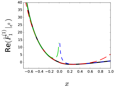
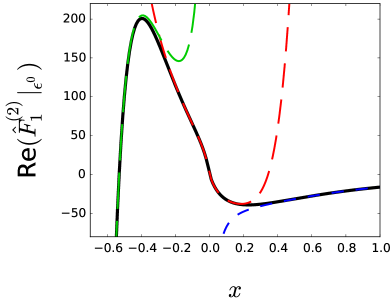
(a)	(b)
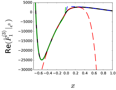
(c)

Figure 6: Panels (a), (b) and (c) show the real part of the $\epsilon^{0}$ term of $\hat{F}_{1}(q^{2})$ at one-, two- and three-loop order, respectively. The solid (black) lines correspond to the exact result and the dashed lines to approximations.

In Fig. 6 the real part of the $\epsilon^{0}$ term of $\hat{F}_{1}(q^{2})$ is shown at one, two and three loops. We show both the exact result (solid, black curve) and the expansions in the three kinematic regions (discussed above) as dashed lines. The approximations contain terms up to order $x^{6}$ and $(1-x)^{6}$ in the high- and low-energy expansion, respectively. At threshold we include terms up to order $\beta^{4}$. The numerical evaluation of the GPLs is performed with the help of ginac [41, 42].

In all three cases one observes strong power-like singularities for $x\to-1$ ($q^{2}\to 4m^{2}$). For this reason we choose $x=-0.7$ as the lower end of the $x$-axes. One observes that the threshold expansion (long-dashed, green curves) reproduces this behaviour and follows the exact curve up to about $x\approx-0.2,-0.3$ and $-0.1$ at one-, two- and three-loop order, respectively. At low energies ($x\to 1$) $\hat{F}^{(n)}_{1}(q^{2})$ shows a smooth behaviour and the corresponding approximation (short-dashed, blue curves) approximate the exact result up to about $x=0.2$. Finally, the region around $x\approx 0$ is nicely covered by the high-energy approximation (medium-sized dashes, red curve) which follows the exact curve from about $x=-0.4$ to $x=0.2$. Altogether for each $x$-value in $[-1,1]$ at least one of the expanded results coincides with the exact curve.

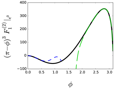
(a)	(b)
(c)

Figure 7: Panels (a), (b) and (c) show the real part of the $\epsilon^{0}$ term of $(\pi-\phi)^{3}F_{1}(q^{2})$ at one-, two- and three-loop order, respectively. The solid (black) lines correspond to the exact result and the dashed lines to approximations.

Fig. 7 shows the real part of the $\epsilon^{0}$ term of $(\pi-\phi)^{3}F_{1}(q^{2})$ at one-, two- and three-loop order as a function of $\phi\in[0,\pi]$, which corresponds to the $q^{2}/m^{2}$ range between 0 and 4. We have introduced the factor $(\pi-\phi)^{3}$ in order to suppress the singularity at threshold ($\phi\to\pi$). In fact, this factor guarantees that the one- and two-loop expressions become zero and the $(\pi-\phi)^{3}F_{1}^{(3)}$ is constant for $\phi=\pi$. As in Fig. 6 we show the exact result as solid line and the low-energy and threshold approximation as short- and long-dashed curves. Good agreement is found for $\phi\lesssim 0.5$ and $\phi\gtrsim 2.0$, respectively, which corresponds to $q^{2}/m^{2}\lesssim 0.24$ and $q^{2}/m^{2}\gtrsim 2.8$. The range inbetween is not covered by our approximations. In principle we could increase the expansion depth, which we refrain to do in this paper.

For $\phi\in[0,\pi]$ the form factors $F_{1}$ and $F_{2}$ have to be real-valued. We have verified this feature numerically which serves as a welcome check for our calculation. Note that the individual GPLs are complex-valued and the imaginary parts only cancel in the sum.

We refrain from showing results for the imaginary part of $F_{1}$ and $F_{2}$, which are obtained in a straightforward way using the expressions in the ancillary file to this paper. We observe qualitatively similar results as in Figs. 6 and 7.

We want to stress that a large part of the $x$ and $\phi$ range is covered by the approximations in the kinematic regions which have a much simpler structure than the exact expressions. Thus, if one wants to have a fast numerical evaluation it is possible to resign to the approximations without essential loss of precision.

6 Conclusions and outlook

In this paper we take the next step in computing massive form factors to three-loop order and compute the complete light-fermion corrections to the massive photon quark form factor. We obtain analytic expressions for $F_{1}$ and $F_{2}$. Our result is expressed in terms of Goncharov polylogarithms with letters $\pm 1$ and $0$. This is the first time that non-planar diagrams have been considered to evaluate massive three-loop vertex functions.

As by-products we compute the two-loop form factors to order $\epsilon^{2}$ and confirm the light-fermion part of the three-loop cusp anomalous dimension.

We expand our exact expressions in the low-energy, threshold, and high-energy limits, and obtain results which are enhanced (for example logarithmically at high energies or by inverse powers of the velocity at threshold) as well as power suppressed terms.

The large-$N_{c}$ results for $F_{1}$ and $F_{2}$, which have been computed in Ref. [2], are also expressed in terms of Goncharov polylogarithms, however, an additional fourth letter, $r_{1}=e^{i\pi/3}$, is required. To complete the evaluation of the massive three-loop corrections to $F_{1}$ and $F_{2}$ one has to consider also non-planar non-fermionic contributions. It is expected that the corresponding analytic result leaves the class of GPLs and elliptic integrals appear. Still, we expect that fast and flexible numerical evaluations of the form factors are possible, e.g., with the help of the strategy presented in Ref. [43].

References

- [1] J. M. Henn, A. V. Smirnov and V. A. Smirnov, JHEP 1612 (2016) 144 [arXiv:1611.06523 [hep-ph]].
- [2] J. Henn, A. V. Smirnov, V. A. Smirnov and M. Steinhauser, JHEP 1701 (2017) 074 [arXiv:1611.07535 [hep-ph]].
- [3] J. M. Henn, A. V. Smirnov, V. A. Smirnov and M. Steinhauser, JHEP 1605 (2016) 066 [arXiv:1604.03126 [hep-ph]].
- [4] J. Henn, A. V. Smirnov, V. A. Smirnov, M. Steinhauser and R. N. Lee, JHEP 1703 (2017) 139 [arXiv:1612.04389 [hep-ph]].
- [5] R. N. Lee, A. V. Smirnov, V. A. Smirnov and M. Steinhauser, Phys. Rev. D 96 (2017) no.1, 014008 [arXiv:1705.06862 [hep-ph]].
- [6] A. von Manteuffel and R. M. Schabinger, Phys. Rev. D 95 (2017) no.3, 034030 [arXiv:1611.00795 [hep-ph]].
- [7] R. H. Boels, T. Huber and G. Yang, Phys. Rev. Lett. 119 (2017) no.20, 201601 [arXiv:1705.03444 [hep-th]].
- [8] R. H. Boels, T. Huber and G. Yang, arXiv:1712.07563 [hep-th].
- [9] W. Bernreuther, R. Bonciani, T. Gehrmann, R. Heinesch, T. Leineweber, P. Mastrolia and E. Remiddi, Nucl. Phys. B 706 (2005) 245 [hep-ph/0406046].
- [10] J. Gluza, A. Mitov, S. Moch and T. Riemann, JHEP 0907 (2009) 001 [arXiv:0905.1137 [hep-ph]].
- [11] T. Ahmed, J. M. Henn and M. Steinhauser, JHEP 1706 (2017) 125 [arXiv:1704.07846 [hep-ph]].
- [12] J. Ablinger, A. Behring, J. Blümlein, G. Falcioni, A. De Freitas, P. Marquard, N. Rana and C. Schneider, arXiv:1712.09889 [hep-ph].
- [13] A. Grozin, Eur. Phys. J. C 77 (2017) no.7, 453 [arXiv:1704.07968 [hep-ph]].
- [14] A. M. Polyakov, Nucl. Phys. B 164 (1980) 171.
- [15] R. A. Brandt, F. Neri and M. a. Sato, Phys. Rev. D 24 (1981) 879.
- [16] G. P. Korchemsky and A. V. Radyushkin, Nucl. Phys. B 283 (1987) 342.
- [17] A. Grozin, J. M. Henn, G. P. Korchemsky and P. Marquard, Phys. Rev. Lett. 114 (2015) no.6, 062006 [arXiv:1409.0023 [hep-ph]].
- [18] A. Grozin, J. M. Henn, G. P. Korchemsky and P. Marquard, JHEP 1601 (2016) 140 [arXiv:1510.07803 [hep-ph]].
- [19] A. V. Smirnov, Comput. Phys. Commun. 189 (2015) 182 [arXiv:1408.2372 [hep-ph]].
- [20] R. N. Lee, arXiv:1212.2685 [hep-ph].
- [21] R. N. Lee, J. Phys. Conf. Ser. 523 (2014) 012059 [arXiv:1310.1145 [hep-ph]].
- [22] A. B. Goncharov, Math. Res. Lett. 5 (1998) 497 [arXiv:1105.2076 [math.AG]].
-
[23]
P. Nogueira,
J. Comput. Phys. 105 (1993) 279;
http://cfif.ist.utl.pt/~paulo/qgraf.html. - [24] J. Kuipers, T. Ueda, J. A. M. Vermaseren and J. Vollinga, Comput. Phys. Commun. 184 (2013) 1453 [arXiv:1203.6543 [cs.SC]].
- [25] R. Harlander, T. Seidensticker and M. Steinhauser, Phys. Lett. B 426 (1998) 125 [hep-ph/9712228].
- [26] T. Seidensticker, hep-ph/9905298.
- [27] A. V. Smirnov and V. A. Smirnov, Comput. Phys. Commun. 184 (2013) 2820 [arXiv:1302.5885 [hep-ph]].
- [28] R. N. Lee, JHEP 1504 (2015) 108 [arXiv:1411.0911 [hep-ph]].
- [29] E. Remiddi and J. A. M. Vermaseren, Int. J. Mod. Phys. A 15 (2000) 725 [hep-ph/9905237].
- [30] R. N. Lee and V. A. Smirnov, JHEP 1102 (2011) 102 [arXiv:1010.1334 [hep-ph]].
-
[31]
https://www.ttp.kit.edu/preprints/2018/ttp18-006/. - [32] A. G. Grozin, P. Marquard, J. H. Piclum and M. Steinhauser, Nucl. Phys. B 789 (2008) 277 [arXiv:0707.1388 [hep-ph]].
- [33] V. V. Sudakov, Sov. Phys. JETP 3 (1956) 65 [Zh. Eksp. Teor. Fiz. 30 (1956) 87].
- [34] J. Frenkel and J. C. Taylor, Nucl. Phys. B 116 (1976) 185.
- [35] A. A. Penin, Phys. Lett. B 745 (2015) 69 Erratum: [Phys. Lett. B 751 (2015) 596] Erratum: [Phys. Lett. B 771 (2017) 633] 10.1016/j.physletb.2015.10.035 [arXiv:1412.0671 [hep-ph]].
- [36] T. Liu, A. A. Penin and N. Zerf, Phys. Lett. B 771 (2017) 492 [arXiv:1705.07910 [hep-ph]].
- [37] T. Liu and A. A. Penin, Phys. Rev. Lett. 119 (2017) no.26, 262001 [arXiv:1709.01092 [hep-ph]].
- [38] A. Pineda and A. Signer, Nucl. Phys. B 762 (2007) 67 [hep-ph/0607239].
- [39] A. H. Hoang, V. Mateu and S. Mohammad Zebarjad, Nucl. Phys. B 813 (2009) 349 [arXiv:0807.4173 [hep-ph]].
- [40] Y. Kiyo, A. Maier, P. Maierhöfer and P. Marquard, Nucl. Phys. B 823 (2009) 269 [arXiv:0907.2120 [hep-ph]].
- [41] C. W. Bauer, A. Frink and R. Kreckel, J. Symb. Comput. 33 (2000) 1 [cs/0004015 [cs-sc]].
- [42] J. Vollinga and S. Weinzierl, Comput. Phys. Commun. 167 (2005) 177 [hep-ph/0410259].
- [43] R. N. Lee, A. V. Smirnov and V. A. Smirnov, arXiv:1709.07525 [hep-ph].