Partitioning of the Free Space-Time for On-Road Navigation of Autonomous Ground Vehicles

Abstract

In this article, we consider the problem of trajectory planning and control for on-road driving of an autonomous ground vehicle (AGV) in presence of static or moving obstacles. We propose a systematic approach to partition the collision-free portion of the space-time into convex sub-regions that can be interpreted in terms of relative positions with respect to a set of fixed or mobile obstacles. We show that this partitioning allows decomposing the NP-hard problem of computing an optimal collision-free trajectory, as a path-finding problem in a well-designed graph followed by a simple (polynomial time) optimization phase for any quadratic convex cost function. Moreover, robustness criteria such as margin of error while executing the trajectory can easily be taken into account at the graph-exploration phase, thus reducing the number of paths to explore.

I Introduction

In order to drive on public roads, autonomous ground vehicles (AGVs) will be required to navigate efficiently inside a potentially dense flow of other vehicles with uncertain behaviors. For this reason, planning safe, efficient and dynamically feasible trajectories that can be safely followed by a low-level controller is a particularly important problem.

One of the difficulties of “optimal” trajectory planning for AGVs is that the presence of obstacles renders the search space non-convex, and multiple possible maneuver variants (for which there is at least one locally optimum trajectory [1]) exist, such as illustrated in Figure 1. At control level, tracking the computed trajectory may involve highly nonlinear vehicle dynamics when nearing the handling limits (see, e.g., [2] for a review); in less demanding (low-slip) scenarios, simpler dynamic models can be used.

Because they allow simultaneous trajectory generation with obstacle avoidance and control computation, model predictive control (MPC) approaches have been very popular for AGVs (see, e.g., [3, 4]). However, real-time constraints usually force authors considering very precise dynamic models to choose a short (sub-second) prediction horizon, which may in turn cause the MPC problem to become infeasible, for instance when a new obstacle is detected with not enough time to stop. Even with simpler dynamic models, the non-convexity of the state-space renders continuous optimization techniques inefficient. For this reason, hierarchical frameworks [5, 6] have been proposed, in which a medium-term (up to a dozen seconds) planner generates a rough trajectory which is then refined by a short-term (sub-second to a few seconds) controller. Mixed-integer programming (MIP) methods are often used in medium-term trajectory planning to encode the discrete decisions arising from multiple maneuver choices [7, 8], generalized as logical constraints in [9]. However, MIP problems are known to be NP-hard [10] and are therefore difficult to solve in real-time.

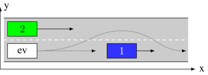
Figure 1: Example driving situation involving multiple maneuver choices for an AGV (denoted ev): overtake the slower (blue, denoted $1$) vehicle before the green vehicle ($2$) passes or wait behind the blue vehicle, possibly overtaking after the green vehicle has passed. Solid arrows represent the velocity of each vehicle, dotted arrows represent possible AGV trajectories.

In this article, we propose a different approach for maneuver selection, inspired by the use of graph-based coordination of robots [11] and the decomposition of the collision-free space presented in [12] for 2D path-planning. First, we introduce a systematic algorithm to partition the collision-free space-time into 3D regions with geometrical adjacency relations; the structure of on-road driving allows to assign a semantic interpretation to each partition subset. Using time discretization, we further divide these regions into convex polyhedrons, and design a transition graph in which any path corresponds to a collision-free trajectory (that may however be dynamically infeasible). The main advantage of our approach is to reduce the entire combinatorial decision-making process (choosing from which side to avoid each obstacle) to the selection of a path in a graph. Once such a path has been selected, we show that computing a corresponding optimal trajectory (for a quadratic convex cost function) in an MPC fashion is widely simplified and can be performed in polynomial time.

A second advantageous property of our decomposition approach is to simplify the use of risk metrics, which can be directly taken into account at the graph exploration phase; in [13], the authors used a similar partitioning technique to design a “space margin” metric for 2D path planning. In this article, we introduce a complementary time margin metric, corresponding to a temporal tolerance to execute a particular maneuver, that can be easily computed from our graph representation. This measure is related to the notion of “gap acceptance”, commonly used in stochastic decision-making (see, e.g., [14]). We believe that combining a temporal margin (notably accounting for uncertainty in predicting the future trajectory of moving obstacles) as well as a spatial margin (accounting for perception and control errors) is key for trajectory planning and tracking in real-world situations, for instance coupled with MPC or Linear Quadratic Gaussian motion planning and control [15].

Our transition graph approach generalizes state-machine-based techniques [16, 17] which rely on a predefined set of maneuvers (such as track lane or change lane) that needs to be manually adapted to the driving situation. By contrast, our method can be applied in many scenarios (including highway and urban driving, for instance crossing an intersection) with the same formalism. Although spatio-temporal graphs have already been used for the control of AGVs [18, 19], no existing approach provides the same desirable properties, and notably to easily account for margins in planning.

The rest of this article is structured as follows: in Section II, we present intuitions of our main ideas using the example scenario of Figure 1. In Section III, we formalize these intuitions mathematically, and we present applications of our results to planning and control for autonomous ground vehicles in Section IV. In Section V, we present early simulation results and data on computation time; finally, Section VI concludes the study.

II A guiding example

The goal of this section is to give an intuition of our main mathematical results using the example scenario shown in Figure 1; the formal mathematical theory is developed in the next section. In our example, we consider an autonomous ground vehicle (called ego-vehicle in the remainder of this article) navigating on a road with two other vehicles (obstacles); vehicles are modeled as rectangles driving parallel to the side of the road. Intuitively, the ego-vehicle has three classes of maneuvers to choose from: either it can remain behind vehicle $1$, overtake it before vehicle $2$ passes, or overtake it after vehicle $2$ has passed; in [1], these maneuver choices are linked to the notion of homotopy classes of trajectories. Assuming that the future trajectory of the obstacles is known in advance, it is possible to compute the obstacle set $\chi_{o}$ of $(x,y,t)$ positions of the ego-vehicle for which a collision exists at time $t$; the complement of this set is the collision-free region of the space-time (or free space-time), denoted by $\chi_{f}$. Any collision-free trajectory for the ego-vehicle corresponds to a path in $\chi_{f}$; Figure 2 provides an illustration of the free space-time in our example.

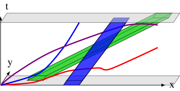
(a)

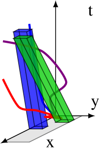
(b)

Figure 2: Free space-time $\chi_{f}$ (in white) corresponding to the situation of Figure 1. Obstacles are pictured in the color of the corresponding vehicle. Light-gray planes represent the road extent in the $y$ direction. The thick curves represent possible collision-free trajectories for the ego-vehicle.

Due to the complex structure of the free space-time, notably its non-convexity, this abstraction is difficult to use directly to compute optimal collision-free trajectories. Inspired by the work in [11] and [12], we propose a decomposition of $\chi_{f}$ in convex subregions with adjacency relations. First, we partition horizontal planes (corresponding to fixed time instants) using relative positions with respect to each obstacle as illustrated in Figure 3. Each subset of the partition corresponds to positions where the ego-vehicle is either located in front ($f$), to the left ($l$), behind ($b$) or to the right ($r$) of each obstacle. Using the additional information given by road boundaries, this partitioning technique yields four subsets denoted by $(lb)$, $(lf)$, $(br)$ and $(fr)$, indicating the relative position of the ego-vehicle from obstacle $1$ and $2$ in this order. We call these labels signature of each subset. Additionally, for two such subsets $A$ and $B$ at a given time $t$, we can define an adjacency relation $\operatorname{adj}_{t}$ (related to that of [12]), such that $\operatorname{adj}_{t}(A,B)=1$ if the intersection of their closures is not empty, i.e. $\bar{A}\cap\bar{B}\neq\emptyset$.

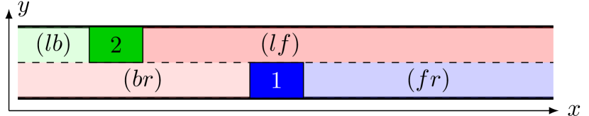
(a) $t=t_{0}$ : $\operatorname{adj}_{t_{0}}(lf,br)=1$, $\operatorname{adj}_{t_{0}}(lb,fr)=0$

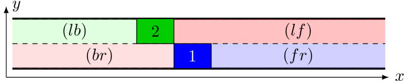
(b) $t=t_{1}$ : $\operatorname{adj}_{t_{1}}(br,lf)=\operatorname{adj}_{t_{1}}(lb,fr)=0$

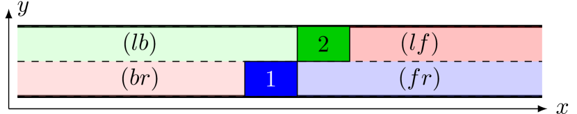
(c) $t=t_{2}$ : $\operatorname{adj}_{t_{2}}(br,lf)=\operatorname{adj}_{t_{2}}(lb,fr)=0$

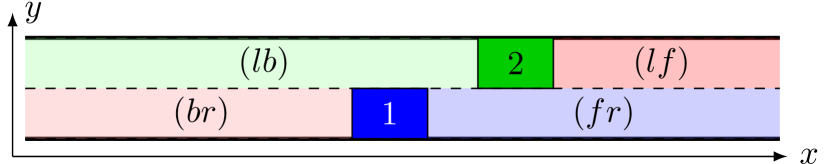
(d) $t=t_{3}$ : $\operatorname{adj}_{t_{3}}(lf,br)=0$, $\operatorname{adj}_{t_{3}}(lb,fr)=1$

Figure 3: Partitioning of the 2D space at different times in our example scenario, and adjacency relations $\operatorname{adj}$. In this example, $\operatorname{adj}_{t}(lb,br)=\operatorname{adj}_{t}(lf,fr)=1$ and $\operatorname{adj}_{t}$ is symmetrical at all times.

This partitioning method can be generalized to the three-dimensional space-time by using unions of regions sharing the same signature, as shown in Figure 4. The notion of adjacency described above can be extended, and we let $\operatorname{Adj}(A,B)$ be the set of times $t$ such that $\operatorname{adj}_{t}(A,B)=1$. We call the set $\operatorname{Adj}(A,B)$ the validity set of the transition from $A$ to $B$, corresponding to time periods for which a collision-free trajectory from $A$ to $B$ exists. The validity sets in this example are given in Table I, with initial time $t_{0}$.

(a)

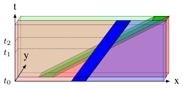
(b)

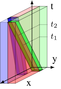
(c)

Figure 4: Partitioning of the free space-time of Figure 2 into four cells. The legend gives the signature of each cell, with blue obstacle first.

Table I: Validity sets $\operatorname{Adj}(A,B)$

	$br$	$fr$	$lb$	$lf$
$br$	$[t_{0},+\infty)$	$\emptyset$	$[t_{0},+\infty)$	$[t_{0},t_{1})$
$fr$	$\emptyset$	$[t_{0},+\infty)$	$(t_{2},+\infty)$	$[t_{0},+\infty)$
$lb$	$[t_{0},+\infty)$	$(t_{2},+\infty)$	$[t_{0},+\infty)$	$\emptyset$
$lf$	$[t_{0},t_{1})$	$[t_{0},+\infty)$	$\emptyset$	$[t_{0},+\infty)$

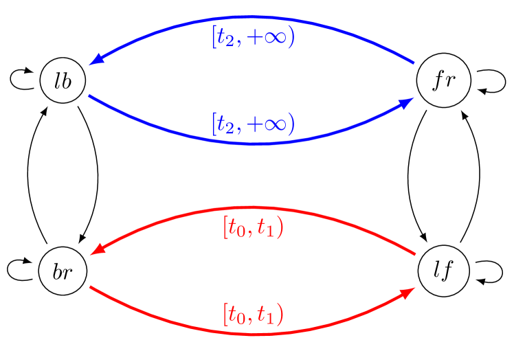
Figure 5: Transition graph corresponding to Figure 4, with validity set of each edge. Thinner edges shown in black have a validity set $[t_{0},+\infty)$ (omitted for readability).

Using Table I, we can build a directed graph (that we call transition graph) representing all the possible transitions between cells of the partition as shown in Figure 5: each vertex of this graph corresponds to a partition cell, and we add the edge $A\rightarrow B$ if $\operatorname{Adj}(A,B)\neq\emptyset$. Additionally, we associate to each edge of the graph the corresponding validity set. A path in this graph is given as a succession of edges and associated transition times within the validity set of each edge, for instance $\left((br\rightarrow lb,t_{1}),(lb\rightarrow fr,t_{2})\right)$ corresponding to the maneuver of waiting for the green vehicle ($2$) to pass before overtaking the blue one ($1$). Between these explicit transition times, the ego-vehicle is supposed to remain inside the last reached cell.

Using this graph-based representation also allows to compute a risk metric associated to a maneuver, called time margin. This measure is defined as the time which remains to the ego-vehicle to perform a particular maneuver, before the most constrained transition becomes impossible. To illustrate this notion (which is formally defined in Section III), we present example time margins for a selection of paths in Table II.

Table II: Time margins of example paths

Path	Most constr. trans.	Margin
$\left((br\rightarrow br,t_{0})\right)$	$br\rightarrow br$	$+\infty$
$\left((br\rightarrow lb,t_{1}),(lb\rightarrow fr,t_{3})\right)$	$lb\rightarrow fr$	$+\infty$
$\left((br\rightarrow lf,t_{0}),(lf\rightarrow fr,t_{1})\right)$	$br\rightarrow lf$	$t_{1}-t_{0}$

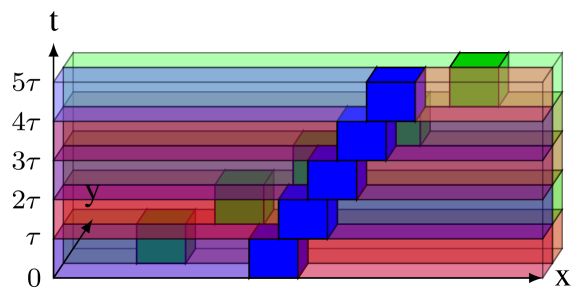
(a)

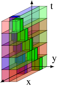
(b)

Figure 6: Discrete partitioning of the free space-time of Figure 2, with $t_{0}=0$.

Figure 7: Discrete-time transition graph and time margins corresponding to the partition of Figure 6. Vertex $A_{k}$ corresponds to the ego-vehicle being in set $A$ at time $t_{0}+k\tau$.

Although this continuous approach is mathematically interesting, it is not necessarily suited for practical computer implementation, which is generally based on time sampling. For this reason, we also propose a discrete partitioning as shown in Figure 6: for a discretization time step $\tau>0$, we approximate the free space as a union of disjointed cylinders of the form $A\times[t_{0}+k\tau,t_{0}+(k+1)\tau)$ where $A$ is a subset in the partition at time $t_{0}+k\tau$. Using this time-discretized partition, we can adapt the notion of adjacency to design a time-discretized transition graph, as shown in Figure 7. In this graph, a path can be simply given as a list of successive vertices, thus allowing to use classic exploration algorithms. The time margin of any edge in the graph can also be easily computed (as shown in Section III). Note that it is also possible to perform an event-based (instead of constant-time-based) partition, which has the advantage of exactly matching the time instants when the adjacency of two cells changes. However, since the partitioning will ultimately be used using the ego-vehicle’s feasible dynamics – which are not easily integrated into an event-based framework – the constant-time discretization is preferred.

We believe that the proposed graph-based representation has two main advantages. First, the combinatorial part of the trajectory planning problem, consisting in choosing a feasible maneuver around the obstacles, is reduced to selecting a path in a transition graph. We will show in Section IV that, once such a path is given, computing a corresponding optimal trajectory becomes relatively simple for a large class of cost functions. Second, the graph approach makes it easy to take into account safety margins by avoiding exploration of time-constrained edges, which can be useful to handle uncertainty in trajectory estimation. Additional metrics can also be computed (see, e.g., [13]) for spatial constraints, in order to account for control or positioning error.

III Mathematical results

III-A Modeling

We now proceed to theorize and generalize the intuitions exposed in the previous section. We consider an autonomous ego ground vehicle, driving on a road in presence of obstacles, which can either be fixed or mobile. The ego-vehicle is assumed to remain parallel to the local direction of the road, as it usually is the case in normal (non-crash) situations, so that its configuration is given by the position of its center of mass, denoted by $(x,y)$ in ground coordinates.

Figure 8: Frenet coordinates of a point on the road.

We assume that the ego-vehicle has knowledge of the road geometry, for instance through cartography, as a $\mathcal{C}^{2}$ reference path $\gamma$ and bounds on the lateral deviation from $\gamma$, as shown in Figure 8; we let $\mathcal{R}\subset\mathbb{R}^{2}$ be such that the ego-vehicle is on the road if, and only if, $(x,y)\in\mathcal{R}$. Finally, we assume that the road curvature and width are such that, for all $X=(x,y)\in\mathcal{R}$, there exists a unique point $X_{\gamma}\in\gamma$ which is closest to $X$.

According to Figure 8, we define the Frenet coordinates of $X$ as $(s(X),r(X))$, where $s(X)$ is the curvilinear position of the corresponding point $X_{\gamma}$ along $\gamma$, and $r(X)=(X-X_{\gamma})\cdot\mathbf{N}$ with $(\mathbf{T},\mathbf{N})$ the Frenet frame of $\gamma$ at point $X_{\gamma}$. With these notations, we let $r_{min}$ and $r_{max}$ be such that $X\in\mathcal{R}$ if, and only if, $r_{min}(s(X))\leq s(X)\leq r_{max}(s(X))$, and we let $\mathcal{Q}=\left\{(s,r)\in\mathbb{R}^{2}\ :r_{min}(s)\leq r\leq r_{max}(s)\right\}$ denote the extent of the road in Frenet coordinates. In what follows, we only consider the Frenet coordinates of the ego-vehicle, and we drop the dependence of $s$ and $r$ in $X$. We assume that the ego-vehicle only moves forward along the road, in the direction of increasing $s$.

We denote by $\mathcal{O}$ the set of obstacles (considered as open sets) existing on the road around the ego-vehicle, and by $N=|\mathcal{O}|$ the number of obstacles. At a given time $t_{0}$, we consider a time horizon $T$ and we assume that an estimation of the trajectory of each obstacle $o\in\mathcal{O}$ is available over $[t_{0},t_{0}+T]$. This estimation could come, for instance, be performed through machine learning techniques [20]. We let $\chi=\mathcal{Q}\times[t_{0},t_{0}+T]$ the set of space-time points for which the vehicle is on the road, and we define the free portions of the space (respectively, of the space-time) as follows:

Definition 1 (Free space)

The (collision-)free space at time $t$ is the set $\mathcal{Q}_{f}^{t}=\mathcal{Q}\setminus\bigcup_{o\in\mathcal{O}}o$. The (collision-)free space-time over $[t_{0},t_{0}+T]$ is the $\chi_{f}=\left\{\mathcal{Q}_{f}^{t}\times{t}\ :\ t\in[t_{0},t_{0}+T]\right\}$.

We call obstacle space-time $\chi_{o}$ the complement of $\chi_{f}$ in $\chi$. Note that the free space-time is similar to the notion of configuration space(-time), which is widely used in robotics [21], and can be computed efficiently [22] provided that each obstacle’s trajectory is known in advance. In this article, we suppose perfect knowledge of these future trajectories over $[t_{0},t_{0}+T]$; however, probabilistic trajectory estimates can also be taken into account, for instance by defining $\chi_{f}^{p}$ as the set of points of $\chi$ which are free with probability $p$.

To simplify the rest of the presentation, we consider that for all $t_{1}\in[t_{0},t_{0}+T]$, the intersection of the obstacle space-time $\chi_{o}$ is a union of (potentially rotated) rectangles; due to the roughly rectangular shape of classical vehicles, this assumption does not excessively sacrifice precision. Moreover, we assume that the road boundary functions $r_{min}$ and $r_{max}$ are piecewise-linear and continuous. In the following subections, we present our approach to partition $\chi_{f}$ into semantically meaningful subsets using a two-step algorithm: first, we partition planes corresponding to a fixed time $t_{1}\in[t_{0},t_{0}+T]$ in Section III-B; second, we deduce a partition of $\chi_{f}$ in Sections III-C and III-D.

III-B Semantic free-space partitioning

Figure 9: Decomposition of the road (in grey) in trapezes.

First, note that we can use trapeze decomposition to partition the road in convex regions using $r_{min}$ and $r_{max}$ as shown in Figure 9; since the road profile does not depend on time, this decomposition allows to fully partition $\chi$ by using cylinders with trapezoidal base. Each trapeze $\mathcal{T}_{k}$ (with $k\in\{1\mathinner{\ldotp\ldotp}K\}$) can be defined by a set of linear constraints, in the form $A_{k}X\leq b_{k}$ with $A_{k}$ a 4-by-2 matrix, $X=[s,r]^{T}$ and $b_{k}$ a vector of $\mathbb{R}^{4}$. This approach allows modeling varying roadway width and curvature, but may require an important number of trapezes to correctly handle sharp bends.

Figure 10: Partitioning of the 2D space around a single obstacle ($C_{o}^{obs}$) into four collision-free regions $C_{o}^{i}$.

For a single rectangular obstacle $o$ at time $t_{1}$, we define four regions $C_{o}^{i}\subset\mathbb{R}^{2}$ ($i\in\{1\mathinner{\ldotp\ldotp}4\}$) as illustrated in Figure 10; as in Section II, these regions can be identified as positions where the ego-vehicle is located in front, to the left, behind or to the right of the obstacle. Similarly, we let $C_{o}^{obs}$ be the obstacle region corresponding to $o$. Since all obstacles are assumed rectangular, each of the $C_{o}^{i}$ regions is defined by a set of linear constraints¹ in the form $A_{o}^{i}X\leq b_{o}^{i}$, with $A_{o}^{i}$ a two-column matrix, $X=[s,r]^{T}$ and $b_{o}^{i}$ a vector having the same number of lines as $A_{o}^{i}$. The partition of the free space $\mathcal{Q}_{f}^{t_{1}}$ can be built recursively according to Algorithm 1; Theorem 1 ensures the validity of this algorithm; we let $\mathcal{P}^{t_{1}}$ be the partition of $\mathcal{Q}_{f}^{t_{1}}$ obtained by Algorithm 1.

Theorem 1 (Partition)

$\mathcal{P}^{t_{1}}$ is a partition of $\mathcal{Q}_{f}^{t_{1}}$.

Proof:

We will prove that, for all $0\leq n\leq N$, $\mathcal{P}_{n}$ is a partition of $\mathcal{Q}_{n}=\mathcal{Q}\setminus\bigcup_{i=1}^{n}C_{o_{i}}^{obs}$. First, this property is verified for $\mathcal{P}_{0}$ which is a partition of $\mathcal{Q}$. Second, the loop preserves the following invariants for all $n\geq 1$ and $e\in\mathcal{P}_{n}$:

• $e\neq\emptyset$ and $\exists e^{\prime}\in\mathcal{P}_{n-1}$ such that $e\subset e^{\prime}$;

• for all $1\leq i\leq n$, $\exists j\in\{1\mathinner{\ldotp\ldotp}4\}$ such that $e\subset C_{o_{i}}^{j}$.

Thus, $\mathcal{P}_{n}=\left\{e\cap C_{o_{n}}^{j}\middle|e\in\mathcal{P}_{n-1},j\in\{1\mathinner{\ldotp\ldotp}4\},e\cap C_{o_{n}}^{j}\neq\emptyset\right\}$. Since the sets $\left(\mathcal{C}_{o_{n}}^{j}\right)_{j=1\mathinner{\ldotp\ldotp}4}$ define a partition of $\mathbb{R}^{2}\setminus C_{o_{n}}^{obs}$ and since all $e\in\mathcal{P}_{0}$ is a subset of $\mathcal{Q}$, we deduce by induction that all elements of $\mathcal{P}_{n}$ are nonempty subsets of $\mathcal{Q}_{n}$.

Reciprocally, for all any $q\in\mathcal{Q}_{n}=\mathcal{Q}_{n-1}\setminus C_{o_{n}}^{obs}$ there exists $j\in\{1\mathinner{\ldotp\ldotp}4\}$ such that $q\in\mathcal{Q}_{n-1}\cap C_{o_{n}}^{j}$. Since $\mathcal{P}_{0}$ is a partition of $\mathcal{Q}$, inductive reasoning yields $\mathcal{Q}_{n}\subset\bigcup_{e\in\mathcal{P}_{n}}e$. ∎

Algorithm 1 Partitioning of $\mathcal{Q}_{f}^{t_{1}}$

$\mathcal{P}_{0}\leftarrow\{\mathcal{T}_{k}\}_{k=1\mathinner{\ldotp\ldotp}K}$ $\triangleright$ Initialize $\mathcal{P}_{0}$ as a partition of $\mathcal{Q}$

$N\leftarrow|\mathcal{O}|$

for $n=1\mathinner{\ldotp\ldotp}N$ do $\triangleright$ Loop over all obstacles $o_{n}$

   $\mathcal{P}_{n}\leftarrow\{\}$

   for all $C\in\mathcal{P}_{n-1}$ do $\triangleright$ Loop over cells $C$ in $\mathcal{P}_{n-1}$

      for $j=1\mathinner{\ldotp\ldotp}4$ do

         if $C_{o_{n}}^{j}\cap C\neq\emptyset$ then $\triangleright$ Partition $C\setminus C_{o_{n}}^{obs}$

            $\mathcal{P}_{n}\leftarrow\mathcal{P}_{n}\cup\{C_{o_{n}}^{j}\cap C\}$

         end if

      end for

   end for

end for

$\mathcal{P}^{t_{1}}\leftarrow\mathcal{P}_{N}$

From the previous proof, we deduce that our partitioning of $\mathcal{Q}_{f}^{t_{1}}$ bijectively corresponds to relative positions from all $N$ obstacles in the free space at time $t_{1}$. Thus, each element in the partition can be uniquely defined by a signature, as stated in Corollary 1 and Definition 2:

Corollary 1 (Semantization)

For all $e\in\mathcal{P}^{t_{1}}$, there exists a unique tuple $\sigma_{t_{1}}(e)=(k,j_{1},\dots,j_{N})\in\{1\mathinner{\ldotp\ldotp}K\}\times\{1\mathinner{\ldotp\ldotp}4\}^{N}$ such that $e=\mathcal{T}_{k}\cap\bigcap_{n=1\mathinner{\ldotp\ldotp}N}C_{o_{n}}^{j_{n}}$. Using $\Sigma=\{1\mathinner{\ldotp\ldotp}K\}\times\{1\mathinner{\ldotp\ldotp}4\}^{N}$, $\sigma_{t_{1}}$ is a bijection from $\Sigma$ to $\mathcal{P}^{t_{1}}\cup\emptyset$.

Definition 2 (Signature)

We call $\sigma_{t_{1}}(e)\in\Sigma$ from Corollary 1 the signature of subset $e$.

Moreover, there is a finite number of elements in the partition which is bounded by $K4^{N}$ for $K$ trapezes and $N$ obstacles. Additionally, all elements $e\in\mathcal{P}^{t_{1}}$ also are convex polygons (or cells), which can be fully described using a single (matrix, vector) pair that can easily be stored in computer memory. Figures 11 and 12 illustrate our partitioning in a more complex scenario with $3$ vehicles; note that, for clarity purposes, we respectively used $f,l,b,r$ instead of $1,2,3,4$ as defined in Definition 2. Also remark that, although Figure 11 is shown in world coordinates $(x,y)$, Figure 12 uses Frenet coordinates $(s,r)$. In order to encode the relation between elements of the partition, we introduce the notion of adjacency as follows:

Definition 3 (Adjacency)

For $e_{1},e_{2}\in\mathcal{P}^{t_{1}}$, we say that $e_{1}$ and $e_{2}$ are adjacent if, and only if the intersection of their closures is not empty, i.e. $\overline{e_{1}}\cap\overline{e_{2}}\neq\emptyset$. For $\sigma,\sigma^{\prime}\in\Sigma$, we let $\operatorname{adj}_{t_{1}}(\sigma,\sigma^{\prime})=1$ if $\sigma_{t_{1}}^{-1}(\sigma)$ and $\sigma_{t_{1}}^{-1}(\sigma^{\prime})$ are adjacent, and $0$ otherwise.

Note that this definition considers cells whose closures intersect at single point as adjacent; this situation could happen, e.g., in the case shown in Figure 3b between (br) and (lf). From a theoretical standpoint, the hypothesis that obstacles are open sets allows to overcome this issue since, in this case, the vehicle can actually perform the maneuver; in practice, the use of safety margins around the obstacles, and constraints on time margin (see Section III-D) prevent this question from becoming an issue. The main reason for choosing this slightly looser criterion compared, e.g., to that of [12] – requiring the intersection to be a non-singleton segment – is that it can be verified in polynomial time using the matrix inequality representation and linear programming.

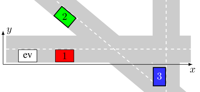
Figure 11: A more complicated example with 3 obstacles.

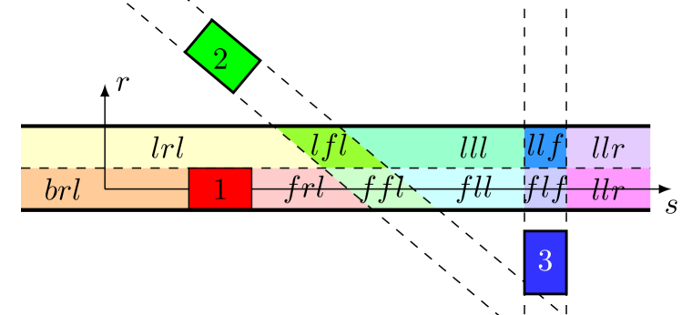
Figure 12: Partitioning in the example of Figure 11, with subsets signature; for instance, $brl$ means that the ego-vehicle is behind the first vehicle, to the right of the second and left of the third. The thick black lines correspond to the unique trapeze encoding road boundaries; its index is omitted for clarity.

III-C Continuous free space-time partitioning

We now proceed to generalize these results to the free space-time $\chi_{f}$; to define a partition of this space we use the union (over time) of cells sharing the same signature:

Definition 4 (Space-time cell)

For $\sigma\in\Sigma$, we let $E_{\sigma}=\bigcup_{t_{1}\in[t_{0},t_{0}+T]}\sigma_{t_{1}}^{-1}(\sigma)\times\{t_{1}\}$ be the space-time cell corresponding to $\sigma$, i.e. the set of all points in the free space-time sharing this signature.

Since the set of non-empty elements of $\sigma_{t}^{-1}(\Sigma)$ defines a partition of $\mathcal{Q}_{f}^{t}$, the set $\mathcal{P}=\left\{E_{\sigma}\,\middle|\,\sigma\in\Sigma,E_{\sigma}\neq\emptyset\right\}$ defines a partition of $\chi_{f}$ (see Figure 4). The notion of adjacency can then be generalized as follows:

Definition 5 (Validity set)

For $\sigma$, $\sigma^{\prime}\in\Sigma$, we define the validity set $\operatorname{Adj}(\sigma,\sigma^{\prime})=\left\{t\in[t_{0},t_{0}+T]\,\middle|\,\operatorname{adj}_{t}(\sigma,\sigma^{\prime})=1\right\}$.

Using this notion, we can now define a transition graph (see Figure 5) as follows:

Definition 6 (Continuous transition graph)

The continuous transition graph is the directed graph $\mathcal{G}^{c}=(\mathcal{V}^{c},\mathcal{E}^{c},\operatorname{Adj})$ with vertex set $\mathcal{V}^{c}=\left\{\sigma\in\Sigma\,\middle|\,E_{\sigma}\neq\emptyset\right\}$, edges set $\mathcal{E}^{c}=\left\{(\sigma_{1},\sigma_{2})\in\Sigma^{2}\,\middle|\,\operatorname{Adj}(E_{\sigma_{1}},E_{\sigma_{2}})\neq\emptyset\right\}$ and associated validity set $\operatorname{Adj}$.

The motivation for introducing this graph is that any collision-free maneuver corresponds to a unique path in $\mathcal{G}^{c}$. To account for the temporal aspect of this graph, such a path is defined as follows:

Definition 7 (Path in $\mathcal{G}^{c}$)

A path in $\mathcal{G}^{c}$ is given by a list of vertices $(\sigma_{1},\dots,\sigma_{m+1})\in\mathcal{V}^{c}$ so that for all $i\leq m$, $(\sigma_{i},\sigma_{i+1})\in\mathcal{E}^{c}$, and a list of strictly increasing transition times $(t_{1},\dots,t_{m})$ such that for all $i\in\{1\mathinner{\ldotp\ldotp}m\}$, $t_{i}\in\operatorname{Adj}(\sigma_{i},\sigma_{i+1})$ and $[t_{i},t_{i+1})\subset\operatorname{Adj}(\sigma_{i},\sigma_{i})$.

In other words, a path in $\mathcal{G}^{c}$ is a sequence of cells and time instants corresponding to the transition time between two successive cells; between two consecutive transitions, the ego-vehicle can remain in the cell it occupies last. For a given path, we can now define the corresponding time margin as the time left for the vehicle to perform the most constrained transition before it becomes impossible:

Definition 8 (Time margin along a path)

Consider a path in $\mathcal{G}^{c}$ given as $\pi^{c}=\big{(}(\sigma_{1},\mathinner{\ldotp\ldotp},\sigma_{m+1}),(t_{1},\mathinner{\ldotp\ldotp},t_{m})\big{)}$. The time margin along $\pi^{c}$ is $V(\pi^{c})=\min_{i=1\dots m}\left(\sup\Big{\{}t-t_{i}\ \big{|}\ [t_{i},t)\subset\operatorname{Adj}(\sigma_{i},\sigma_{i+1})\Big{\}}\right)$.

III-D Discrete-time partitioning

Due to the potentially complex trajectories followed by the obstacles, there is no guarantee regarding the topology of the subsets $E_{\sigma}$, which can for instance have multiple connected components; similarly, $\operatorname{Adj}(\sigma_{1},\sigma_{2})$ is in general a union of disjointed intervals. To make practical applications easier, we also propose a temporal discretization of the free space-time with a time step duration $\tau$ (with $T=P\tau$). Note that the value of $\tau$ depends on a trade-off between acceptable computation time, length of the planning horizon and required precision in vehicle dynamics; Section V provides some performance reports on the influence of this parameter. We approximate $E_{\sigma}$ as a union of box-shaped cells:

Definition 9 (Discrete space-time cell)

For $\sigma\in\Sigma$ and $p\in\{0\dots P\}$, we let $E_{\sigma}^{p}=\sigma_{\theta_{p}}^{-1}(\sigma)\times[\theta_{p},\theta_{p+1})$ be the discrete space-time cell corresponding to $\sigma$ at step $p$, with $\theta_{p}=t_{0}+p\tau$.

In the rest of this article, we assume that $E_{\sigma}^{p}\subset\chi_{f}$ for all $\sigma\in\Sigma$ and $p\in\{0\mathinner{\ldotp\ldotp}P\}$. Since $\sigma_{\theta_{p}}^{-1}(\sigma)$ is a convex (or empty) set, $E_{\sigma}^{p}$ is either empty or convex, and fully defined by a set of linear inequalities in the form $A[X,t]^{T}\leq b$ (the comments of footnote 1 also apply here). Finally, we define a partition of the free space-time $\chi_{f}$ in convex box-shaped cells as $\mathcal{P}^{\tau}=\left\{E_{\sigma}^{p}\middle|p\in\{0\mathinner{\ldotp\ldotp}P\},\sigma\in\Sigma,E_{\sigma}^{p}\neq\emptyset\right\}$ (see Figure 6), and we associate a discrete transition graph:

Definition 10 (Discrete transition graph)

The discrete transition graph is the directed graph $\mathcal{G}^{d}=(\mathcal{V}^{d},\mathcal{E}^{d})$ with vertex set $\mathcal{V}^{d}=\mathcal{P}^{\tau}$ and edges set $\mathcal{E}^{d}=\left\{(E_{\sigma_{1}}^{p},E_{\sigma_{2}}^{p+1})\middle|E_{\sigma_{1}}^{p},E_{\sigma_{2}}^{p+1}\in\mathcal{V}^{d},\,\operatorname{adj}_{\theta_{p}}(\sigma_{1},\sigma_{2})=1\right\}$.

Therefore, each vertex of $\mathcal{G}$ corresponds to a certain cell of the partition $\mathcal{P}^{\tau}$ at a given time $\theta_{p}$, and the edge $v_{1}\rightarrow v_{2}$ exists if $v_{1}$ and $v_{2}$ represent two adjacent cells (possibly twice the same) at two consecutive time steps. Paths in $\mathcal{G}^{d}$ comply with the usual definitions of graph theory and can be given as a set of vertices.

Finally, we define the time margin for paths in $\mathcal{G}^{d}$ as:

Definition 11 (Time margin in the discrete graph)

For a path $\pi^{d}=\big{(}E_{\sigma_{0}}^{0},\dots,E_{\sigma_{m+1}}^{m+1}\big{)}$ in $\mathcal{G}^{d}$, the time margin is $v(\pi^{d})=\displaystyle{\min_{i=0\dots m}}\max_{p=i\dots m}\tilde{v}(i,p)$ with $\tilde{v}(i,p)=\big{\{}\tau(p-i+1)\,\big{|}\,\forall q\in\{i\mathinner{\ldotp\ldotp}p\},\operatorname{adj}_{\theta_{q}}(\sigma_{i},\sigma_{i+1})=1\big{\}}$.

Note that $\tilde{v}(i,p)$ is the discrete-time equivalent of the set $\left\{t-t_{i}\ \big{|}\ [t_{i},t)\subset\operatorname{Adj}(\sigma_{i},\sigma_{i+1})\right\}$ from Definition 8, and this discrete time margin is analogous to that of Definition 8.

IV Application to planning and control

Before presenting the applications of our approach to planning and control, let us formalize the link between paths in the transition graph and trajectories for the ego-vehicle:

Definition 12 (Interpretation of transition graph paths)

Let $\pi_{0}^{c}=\big{(}(\sigma_{1},\dots,\sigma_{m+1}),(t_{1},\dots,t_{m})\big{)}$ be a path in $\mathcal{G}^{c}$ and $x(t)$ be a collision-free trajectory for the ego-vehicle. We say that $\pi_{0}$ corresponds to $x$ if, for all $i\in\{1\mathinner{\ldotp\ldotp}m\}$, $x\big{(}[t_{i-1},t_{i})\big{)}\subset E_{\sigma_{i}}$ and $x\big{(}[t_{m},T)\big{)}\subset E_{\sigma_{m+1}}$.

From this definition, we deduce that for a given collision-free trajectory $x(t)$ there exists a unique corresponding path in $\mathcal{G}^{c}$ denoted by $\pi(x)$. Reciprocally, for a given path $\pi_{0}$ in $\mathcal{G}^{c}$, there exists a set of corresponding trajectories denoted by $\pi^{-1}(\pi_{0})$. We obtain the following theorem:

Theorem 2 (Motion-planning equivalence)

Let $J(x)$ be a cost function for a given trajectory $x(t)$, $X$ the set of collision-free trajectories, and $\Pi$ the set of paths in $\mathcal{G}^{c}$. Then:

$$\min_{x\in X}J(x)=\min_{\pi_{0}\in\Pi}\left(\min_{x\in\pi^{-1}(\pi_{0})}J(x)\right)$$ (1)

Proof:

From the previous definition, for any collision-free trajectory $x\in X$ there exists $\pi_{0}\in\Pi$ such that $\pi(x)=\pi_{0}$. Therefore, $\min_{x\in X}J(x)\leq\min_{\pi_{0}\in\Pi}\left(\min_{x\in\pi^{-1}(\pi_{0})}J(x)\right)$. Reciprocally, for all $\pi_{0}\in\Pi$, any $x\in\pi^{-1}(\pi_{0})$ is guaranteed to be collision-free, leading to the reciprocal inequality. ∎

In other words, it is equivalent to find an optimal trajectory for the ego-vehicle, and to find an optimal path in the transition graph $\mathcal{G}^{c}$ and then the optimal trajectory corresponding to this path. These results can be extended to paths in the discrete graph $\mathcal{G}^{d}$; due to space limitations, details are not presented here and we only provide the following definition:

Definition 13 (Interpretation of discrete graph paths)

Let $\tau>0$ be a discretization time step, $\pi_{0}^{d}=(E_{\sigma_{0}}^{0},\dots,E_{\sigma_{m+1}}^{m+1})$ be a path in $\mathcal{G}^{d}$ and $x(t)$ be a collision-free trajectory for the ego-vehicle. We say that $\pi_{0}^{d}$ corresponds to $x$ if, for all $p\in\{0\mathinner{\ldotp\ldotp}m\}$, $x(\theta_{p})\in E_{\sigma_{p}}^{p}$ and $x([\theta_{p},\theta_{p+1}))\subset E_{\sigma_{p}}^{p}\cup E_{\sigma_{p+1}}^{p}$.

An interesting feature of this decomposition of the trajectory planning problem is that we effectively separate the discrete choice of a maneuver variant, and the search for an optimal control corresponding to this maneuver as was obtained in [12] for path-planning. This second problem can be solved efficiently under certain assumptions on the vehicle dynamics. We consider an AGV with linear discrete dynamics $x_{p+1}=Ax_{p}+Bu_{p}$ for a state $x_{p}$ and a control $u_{p}\in U$ (with $U$ a convex polyhedron) with a discretization time step $\tau$, where $A$ and $B$ have constant coefficient. For a positive semi-definite matrix $Q$, a line vector $L$ and defining $X_{p}=[x_{p}^{T},u_{p}^{T}]^{T}$, we consider a generic quadratic cost function $J(x,u)=\frac{1}{2}X_{p}^{T}QX_{p}+L^{T}X_{p}$. In this case, an optimal solution can be computed in polynomial time:

Theorem 3 (Polynomial time computability)

Let $\pi_{0}$ be a path in $\mathcal{G}^{d}$ and $x_{0}$ an initial AGV state. The optimal trajectory (and associated control sequence) $(X_{p})$ starting from $x_{0}$ realizing $\displaystyle\min_{(x_{p})\in\pi^{-1}(\pi_{0}),u_{p}\in U}J(x,u)$ can be computed in polynomial time in the number of obstacles and time steps.

Proof:

We will show that this problem is an instance of convex quadratic programming (QP), which has a complexity $\mathcal{O}(n^{3})$ where $n$ is the number of constraints [23]. First, the cost function $J$ is quadratic and convex. Second, vehicle dynamics and control bounds can be encoded as linear constraints. Moreover, the condition $(x_{p})\in\pi^{-1}(\pi_{0})$ corresponds to a set of $\mathcal{O}(PN)$ linear constraints, leading to a QP problem with complexity $\mathcal{O}\left((PN)^{3}\right)$ for $N$ obstacles over $P$ time steps, thus proving the announced result. ∎

V Simulation results

To showcase the advantages of our approach and the axes for improvement, we present preliminary simulation results in the scenario of Figure 1. For illustration purposes, we consider a very simple second-order dynamics for the ego-vehicle as: $X_{p+1}=\left(\begin{smallmatrix}0&I_{2}\\ 0&0\end{smallmatrix}\right)X_{p}+\left(\begin{smallmatrix}0\\ I_{2}\end{smallmatrix}\right)u_{p}$ with $X_{p}=[s,r,\dot{s},\dot{r}]_{p}^{T}$, $u_{p}=[a_{lon},a_{lat}]_{p}^{T}$ and $I_{2}$ the $\mathbb{R}^{2}$ identity. To account for the nonholonomic constraints, we bound the lateral velocity as $|\dot{r}_{p}|\leq\alpha\dot{s}_{p}$ with $\alpha>0$ a parameter, and we also require $a_{lon}$ and $a_{lat}$ to be bounded. The objective function is chosen as $J=\sum_{p}\left(\dot{s}_{p}-s_{p}^{ref}\right)^{2}+\dot{r}_{p}^{2}+r_{p}^{2}$, and we use a planning horizon of $10\text{\,}\mathrm{s}$ with a time step $\tau=$1\text{\,}\mathrm{s}$$, and a minimum time margin of $1\text{\,}\mathrm{s}$.

One difficulty in the proposed approach is the need to ensure that the selected optimal path in the transition graph is dynamically feasible. In this early implementation, we use a naive approach consisting in computing the optimal trajectory corresponding to each explored branch; as stated in Theorem 3, this computation can be performed relatively fast. Additionally, we use a branch-and-bound technique to prune dynamically infeasible or poor quality branches. The trajectories from both algorithms are shown in Figure 13; Table III reports the computation time for all steps of our algorithm using a standard desktop computer. For comparison purposes, we added an implementation of the same problem using a pure mixed-integer quadratic programming (MIQP) method from [9]. We use an implementation of Seidel’s linear programming algorithm [24] to perform the partitioning, and Gurobi [25] in version 7.5 to solve quadratic programming (trajectory optimization) and MIQP (from [9]) problems.

Although the MIQP is faster overall, it is not able to take notions such as time margin into account; this results in the ego-vehicle trying to overtake the blue vehicle (1) before the green one (2), which is a higher-risk maneuver that is excluded by our algorithm as shown in Figure 13; when removing the time margin constraints, both solvers converge to the same optimum. A likely explanation for the better performance of the pure MIQP method is that it can directly use vehicle dynamics to guide the exploration; future work will focus on designing an hybrid algorithm between these methods, to benefit from the advantages of both approaches.

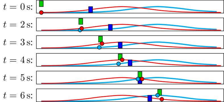
Figure 13: Trajectories computed by both algorithms (MIQP in red, our graph-based approach in thicker cyan) for a time margin of $1\text{\,}\mathrm{s}$. The rectangles correspond to the vehicles of Figure 1; the circles to the ego-vehicle position.

Table III: Summary of computation time (average over 100 iterations)

Algorithm	Comp. time	Objective val.
Partitioning	$2.5\text{\,}\mathrm{ms}$	-
Graph exploration ($1\text{\,}\mathrm{s}$ margin)	$27.6\text{\,}\mathrm{ms}$	13.89
Optimal path computation	$<$1\text{\,}\mathrm{ms}$$	-
MIQP [9]	$14.0\text{\,}\mathrm{ms}$	13.58
Our graph exploration (no margin)	$28.4\text{\,}\mathrm{ms}$	13.58

VI Conclusion

This article generalized the divide-and-conquer approach used in [12] in two dimensions, to the 3D space-time for on-road navigation of autonomous ground vehicles in presence of moving obstacles. We described a systematic method to partition the collision-free space-time in the presence of fixed or moving obstacles, and we provided a graph representation of all possible collision-free trajectories. This approach allows to treat the combinatorial problem of optimal trajectory planning in two steps: first, a path-finding problem in a graph, and then a simple optimization that can be performed in polynomial time in the number of obstacles for any quadratic cost function. Moreover, we introduced a notion of time margin and showed that our graph-based approach can easily take into account margin of error in the execution for a particular maneuver. Coupled with additional similar metrics, we believe that our approach can have useful applications for planning under prediction and control uncertainty, notably in the frame of stochastic decision-making. Future work will also focus on improving our graph exploration algorithm to allow faster computation.

References

- [1] P. Bender, O. S. Tas, J. Ziegler, and C. Stiller, “The Combinatorial Aspect of Motion Planning: Maneuver Variants in Structured Environments,” pp. 1386–1392, 2015.
- [2] J. Kong, M. Pfeiffer, G. Schildbach, and F. Borrelli, “Kinematic and dynamic vehicle models for autonomous driving control design,” in 2015 IEEE Intelligent Vehicles Symposium (IV). IEEE, jun 2015, pp. 1094–1099.
- [3] P. Falcone, F. Borrelli, J. Asgari, H. E. Tseng, and D. Hrovat, “A model predictive control approach for combined braking and steering in autonomous vehicles,” in 2007 Mediterranean Conference on Control & Automation. IEEE, jun 2007, pp. 1–6.
- [4] M. A. Abbas, R. Milman, and J. M. Eklund, “Obstacle avoidance in real time with Nonlinear Model Predictive Control of autonomous vehicles,” in 2014 IEEE 27th Canadian Conference on Electrical and Computer Engineering (CCECE). IEEE, may 2014, pp. 1–6.
- [5] R. V. Cowlagi and P. Tsiotras, “Hierarchical motion planning with kinodynamic feasibility guarantees: Local trajectory planning via model predictive control,” in 2012 IEEE International Conference on Robotics and Automation. IEEE, may 2012, pp. 4003–4008.
- [6] X. Qian, A. De La Fortelle, and F. Moutarde, “A hierarchical model predictive control framework for on-road formation control of autonomous vehicles,” in Intelligent Vehicles Symposium (IV), 2016 IEEE. IEEE, 2016, pp. 376–381.
- [7] T. Schouwenaars, É. Féron, and J. How, “Safe receding horizon path planning for autonomous vehicles,” Proceedings of the Annual Allerton Conference on Communication Control and Computing, vol. 40, no. 1, pp. 295–304, 2002.
- [8] S. J. Anderson, S. C. Peters, T. E. Pilutti, and K. Iagnemma, “Design and development of an optimal-control-based framework for trajectory planning, threat assessment, and semi-autonomous control of passenger vehicles in hazard avoidance scenarios,” Springer Tracts in Advanced Robotics, vol. 70, no. STAR, pp. 39–54, 2011.
- [9] X. Qian, F. Altché, P. Bender, C. Stiller, and A. de La Fortelle, “Optimal trajectory planning for autonomous driving integrating logical constraints: An MIQP perspective,” in 2016 IEEE 19th International Conference on Intelligent Transportation Systems (ITSC). IEEE, nov 2016, pp. 205–210.
- [10] R. M. Karp, “Reducibility among combinatorial problems,” in Complexity of computer computations. Springer, 1972, pp. 85–103.
- [11] J. Gregoire, S. Bonnabel, and A. de La Fortelle, “Priority-based intersection management with kinodynamic constraints,” in 2014 European Control Conference (ECC). IEEE, jun 2014, pp. 2902–2907.
- [12] J. Park, S. Karumanchi, and K. Iagnemma, “Homotopy-Based Divide-and-Conquer Strategy for Optimal Trajectory Planning via Mixed-Integer Programming,” IEEE Transactions on Robotics, vol. 31, no. 5, pp. 1101–1115, 2015.
- [13] A. Constantin, J. Park, and K. Iagnemma, “A margin-based approach to threat assessment for autonomous highway navigation,” in 2014 IEEE Intelligent Vehicles Symposium Proceedings, vol. 12, no. 4. IEEE, jun 2014, pp. 234–239.
- [14] S. Lefevre, C. Laugier, and J. Ibanez-Guzman, “Evaluating risk at road intersections by detecting conflicting intentions,” in 2012 IEEE/RSJ International Conference on Intelligent Robots and Systems. IEEE, oct 2012, pp. 4841–4846.
- [15] J. van den Berg, P. Abbeel, and K. Goldberg, “LQG-MP: Optimized path planning for robots with motion uncertainty and imperfect state information,” The International Journal of Robotics Research, vol. 30, no. 7, pp. 895–913, jun 2011.
- [16] Q. Wang, T. Weiskircher, and B. Ayalew, “Hierarchical Hybrid Predictive Control of an Autonomous Road Vehicle,” in 2015 Dynamic Systems and Control Conference. ASME, oct 2015.
- [17] Q. Wang, B. Ayalew, and T. Weiskircher, “Optimal assigner decisions in a hybrid predictive control of an autonomous vehicle in public traffic,” Proceedings of the American Control Conference, vol. 2016-July, pp. 3468–3473, 2016.
- [18] M. Ono, G. Droge, H. Grip, O. Toupet, C. Scrapper, and A. Rahmani, “Road-following formation control of autonomous ground vehicles,” in 2015 54th IEEE Conference on Decision and Control (CDC), no. Cdc. IEEE, dec 2015, pp. 4714–4721.
- [19] T. Gu, J. Atwood, C. Dong, J. M. Dolan, and Jin-Woo Lee, “Tunable and stable real-time trajectory planning for urban autonomous driving,” in 2015 IEEE/RSJ International Conference on Intelligent Robots and Systems (IROS). IEEE, sep 2015, pp. 250–256.
- [20] F. Altché and A. de La Fortelle, “An LSTM network for highway trajectory prediction,” in Intelligent Transportation Systems (ITSC), 2017 IEEE 19th International Conference on. IEEE, 2017.
- [21] M. Erdmann and T. Lozano-Perez, “On multiple moving objects,” in Robotics and Automation. Proceedings. 1986 IEEE International Conference on, vol. 3. IEEE, 1986, pp. 1419–1424.
- [22] S. Kockara, T. Halic, K. Iqbal, C. Bayrak, and R. Rowe, “Collision detection: A survey,” in Systems, Man and Cybernetics, 2007. ISIC. IEEE International Conference on. IEEE, 2007, pp. 4046–4051.
- [23] S. A. Vavasis, Complexity theory: quadratic programming Complexity Theory: Quadratic Programming. Boston, MA: Springer US, 2009, pp. 451–454.
- [24] R. Seidel, “Small-dimensional linear programming and convex hulls made easy,” Discrete & Computational Geometry, vol. 6, no. 1, pp. 423–434, 1991.
- [25] Gurobi Optimization, Inc., “Gurobi optimizer reference manual,” 2017.