Gaussian variational approximations for high-dimensional state space models

Abstract

Our article considers a Gaussian variational approximation of the posterior density in a high-dimensional state space model. The variational parameters to be optimized are the mean vector and the covariance matrix of the approximation. The number of parameters in the covariance matrix grows as the square of the number of model parameters, so it is necessary to find simple yet effective parameterizations of the covariance structure when the number of model parameters is large. We approximate the joint posterior distribution over the high-dimensional state vectors by a dynamic factor model, having Markovian time dependence and a factor covariance structure for the states. This gives a reduced description of the dependence structure for the states, as well as a temporal conditional independence structure similar to that in the true posterior. The usefulness of the approach is illustrated for prediction in two high-dimensional applications that are challenging for Markov chain Monte Carlo sampling. The first is a spatio-temporal model for the spread of the Eurasian Collared-Dove across North America; the second is a Wishart-based multivariate stochastic volatility model for financial returns.
Keywords. Dynamic factor, Stochastic gradient, Spatio-temporal modeling.

1 Introduction

Variational Approximation (VA) (Ormerod and Wand,, 2010; Blei et al.,, 2017) estimates the posterior distribution of a model by assuming the form for the posterior density and optimizing a measure of closeness to the true posterior; e.g., a frequent choice for the approximation is a multivariate Gaussian distribution, where the variational optimization is over an unknown mean and covariance matrix. VA is becoming an increasingly popular way to estimate the posterior because of its ability to handle large datasets and highly parameterized models. The accuracy of the VA depends on a number of factors, such as the flexibility of the approximating family, the model considered, and the sample size. There are now some theoretical results which show that the variational posterior converges to the true parameter value under suitable regularity conditions, and rates of convergence have been established for parametric models (Wang and Blei,, 2019) and, more generally, for non-parametric and high-dimensional models (Zhang and Gao,, 2018). However, for a finite number of observations, when the variational approximation does not collapse to a point mass, it is often observed that there is a practically meaningful discrepancy between the uncertainty quantification provided by the approximation and that of the true posterior distribution. This is especially the case when the variational family used is insufficiently flexible. Nevertheless, even in these cases, predictive inference – predictions and prediction intervals – obtained from VA seem empirically to be usefully close to those obtained from the exact posterior. As such, variational approximation methods provide a useful and fast alternative to Markov chain Monte Carlo (MCMC), especially when predictive inference is the focus of the analysis.

Our article considers a Gaussian variational approximation (GVA) for a state space model when the state vector is high-dimensional. Such models are common in spatio-temporal applications (Cressie and Wikle,, 2011), financial econometrics (Philipov and Glickman, 2006b, ), and in other important applications. It is challenging to obtain the GVA when dealing with a high-dimensional model, because the number of variational parameters in the covariance matrix of the VA grows quadratically with the number of model parameters. This makes it necessary to parameterize the variational covariance matrix parsimoniously, but still be able to capture the structure of the posterior. This goal is best achieved by taking into account the structure of the posterior itself. We do so by parameterizing the variational posterior covariance matrix using a dynamic factor model, which reduces the dimension of the state vector. The Markovian time dependence for the low-dimensional factors provides sparsity in the precision matrix for the factors.

We develop efficient computational methods for forming the approximations and illustrate the advantages of the approach in two high-dimensional example datasets. For both models, Bayesian inference by MCMC simulation is challenging. The first is a spatio-temporal model for the spread of the Eurasian collared dove across North America (Wikle and Hooten,, 2006); the second is a multivariate stochastic volatility model for a collection of portfolios of assets (Philipov and Glickman, 2006b, ). We derive GVAs for both models and show that they give useful predictive inference.

VA estimates the posterior by optimization. Our article uses stochastic gradient ascent methods to performing the optimization (Ji et al.,, 2010; Nott et al.,, 2012; Paisley et al.,, 2012; Salimans and Knowles,, 2013). In particular, the so-called reparameterization trick is used to unbiasedly estimate the gradients of the variational objective (Kingma and Welling,, 2014; Rezende et al.,, 2014). Section 2 briefly reviews these methods. Applying these methods for GVA, Tan and Nott, (2017) match the sparsity of the variational precision matrix to the conditional independence structure of the true posterior based on a sparse Cholesky factor for the precision matrix. Their motivation is that zeros in the precision matrix of a Gaussian distribution correspond to conditional independence between variables, and sparse matrix operations allow computations in the variational optimization to be done efficiently. They apply their approach to both random effects models and state space models, but their method is impractical for a state space model having a high-dimensional state vector. This approach and related approximations using a sparse precision matrix are reviewed further in Section 3.

Our approach is also related to recent high-dimensional Gaussian posterior approximations having a factor structure. Factor models (Bartholomew et al.,, 2011) are well known to be useful for modeling dependence in high-dimensional settings. Ong et al., (2018) consider a Gaussian variational approximation for factor covariance structures using stochastic gradient methods for the variational optimization. Computation in the variational optimization can be done efficiently in high dimensions using the Woodbury formula (Woodbury,, 1950). Barber and Bishop, (1998) and Seeger, (2000) used factor structures in GVA, but only when the variational objective can be computed analytically or with one-dimensional quadrature. Rezende et al., (2014) consider a factor model for the precision matrix with one factor in some applications to some deep generative models arising in machine learning applications. Miller et al., (2017) considered factor parameterizations of covariance matrices for normal mixture components in a flexible variational boosting approximate inference method, including a method for exploiting the reparameterization trick for unbiased gradient estimation of the variational objective in that setting.

Various other parameterizations of the covariance matrix in GVA were considered by Opper and Archambeau, (2009), Challis and Barber, (2013) and Salimans and Knowles, (2013). Salimans and Knowles, (2013) also considered efficient stochastic gradient methods for fitting such approximations, using both gradient and Hessian information and exploiting other structure in the target posterior distribution, as well as extensions to more complex hierarchical formulations including mixtures of normals.

Our article makes use of both the conditional independence structure and the factor structure in forming the GVA for high dimensional state space models. Bayesian computations for state space models are well known to be challenging for complex nonlinear models. It is usually feasible to carry out MCMC on a complex state space model by sampling the states one at a time conditional on the neighbouring states (e.g., Carlin et al.,, 1992); in general, sampling one state at a time requires careful convergence diagnosis and can fail if the dependence between states is strong. Carter and Kohn, (1994) document this phenomenon in linear Gaussian state space models, and we also document this problem of poor mixing for the spatio-temporal case (Wikle and Hooten,, 2006) discussed later.

State-of-the-art general approaches using particle MCMC methods (Andrieu et al.,, 2010) can in principle be much more efficient than an MCMC algorithm that generates the states one at a time. However, particle MCMC is usually much slower than MCMC because of the need to generate multiple particles at each time point. Particle methods also have a number of other drawbacks, which depend on the model that is estimated. Thus, if there is strong dependence between the states and parameters, then it is necessary to use pseudo-marginal methods (Beaumont,, 2003; Andrieu and Roberts,, 2009) which estimate the likelihood and it is necessary to ensure that the variability of the log of the estimated likelihood is sufficiently small (Pitt et al.,, 2012; Doucet et al.,, 2015). This is particularly difficult to do if the state dimension is high.

The rest of the article is organized as follows. Section 2 provides a brief description of variational approximation. Section 3 reviews some previous parameterizations of the covariance matrix, in particular the methods of Tan and Nott, (2017) and Ong et al., (2018) for GVA using conditional independence and a factor structure, respectively. Section 4 describes our methodology, which combines a factor structure for the states and conditional independence in time for the factors to obtain flexible and convenient approximations of the posterior distribution in high dimensional state space models. Section 5 describes an extended example for a spatio-temporal dataset in ecology concerned with the spread of the Eurasian collared-dove across North America. Section 6 considers variational inference in a Wishart based multivariate stochastic volatility model. Appendix A contains the necessary gradient expressions to implement our method. Technical derivations and other details are placed in a self-contained supplement after the main article. We refer to equations, sections, etc in the main paper as (1), Section 1, etc, and in the supplement as (S1), Section S1, etc.

2 Stochastic gradient variational methods

2.1 Variational objective function

Variational approximation methods (Attias,, 1999; Jordan et al.,, 1999; Winn and Bishop,, 2005) reformulate the problem of approximating an intractable posterior distribution as an optimization problem. Let $\theta=(\theta_{1},\dots,\theta_{d})^{\top}$ be the vector of model parameters, $y=(y_{1},\dots,y_{n})^{\top}$ the observations and consider Bayesian inference for $\theta$ with a prior density $p(\theta)$. Denoting the likelihood by $p(y|\theta)$, the posterior density is $p(\theta|y)\propto p(\theta)p(y|\theta)$, and in variational approximation we consider a family of densities $\{q_{\lambda}(\theta)\}$, indexed by the variational parameter $\lambda$, to approximate $p(\theta|y)$. Our article takes the approximating family to be Gaussian so that $\lambda$ consists of the mean vector and the distinct elements of the covariance matrix in the approximating normal density.

To express the approximation of $p(\theta|y)$ as an optimization problem, we take the Kullback-Leibler (KL) divergence,

$$\mathrm{KL}(q_{\lambda}(\theta)||p(\theta|y)) =\int\log\frac{q_{\lambda}(\theta)}{p(\theta|y)}q_{\lambda}(\theta)\;d\theta,$$

as the discrepancy measure between $q_{\lambda}(\theta)$ to $p(\theta|y)$. The KL divergence is non-negative and zero if and only if $q_{\lambda}(\theta)=p(\theta|y)$. It is straightforward to show that $\log p(y)$, where $p(y)=\int p(\theta)p(y|\theta)\;d\theta$, can be expressed as

$$\log p(y) ={\cal L}(\lambda)+\mathrm{KL}(q_{\lambda}(\theta)||p(\theta|y)),$$ (1)

where

$${\cal L}(\lambda) =\int\log\frac{p(\theta)p(y|\theta)}{q_{\lambda}(\theta)}q_{\lambda}(\theta)\;d\theta$$ (2)

is referred to as the variational lower bound or evidence lower bound (ELBO). We have that $\log p(y)\geq{\cal L}(\lambda)$, with equality if and only if $q_{\lambda}(\theta)=p(\theta|y)$ because the KL divergence is non-negative. Eq. (1) shows that minimizing the KL divergence is equivalent to maximizing the ELBO in (2) because $\log p(y)$ does not depend on $\lambda$; this is a more convenient optimization target as it does not involve the intractable $p(y)$.

For introductory overviews of variational methods for statisticians see Ormerod and Wand, (2010); Blei et al., (2017).

2.2 Stochastic gradient optimization

Maximizing ${\cal L}(\lambda)$ to obtain an optimal approximation of $p(\theta|y)$ is often difficult in models with a non-conjugate prior structure, since ${\cal L}(\lambda)$ is defined as an integral which is generally intractable. However, stochastic gradient methods (Robbins and Monro,, 1951) are useful for performing the optimization and there is now a large literature surrounding the application of this idea (Ji et al.,, 2010; Paisley et al.,, 2012; Nott et al.,, 2012; Salimans and Knowles,, 2013; Kingma and Welling,, 2014; Rezende et al.,, 2014; Hoffman et al.,, 2013; Ranganath et al.,, 2014; Titsias and Lázaro-Gredilla,, 2015; Kucukelbir et al.,, 2017, among others). In a simple stochastic gradient ascent method for optimizing ${\cal L}(\lambda)$, an initial guess for the optimal value $\lambda^{(0)}$ is updated according to the iterative scheme

$$\lambda^{(t+1)} =\lambda^{(t)}+a_{t}\widehat{\nabla_{\lambda}{\cal L}(\lambda^{(t)})},$$ (3)

where $a_{t}$, $t\geq 0$ is a sequence of learning rates; $\nabla_{\lambda}{\cal L}(\lambda)$ is the gradient vector of ${\cal L}(\lambda)$ with respect to $\lambda$; and $\widehat{\nabla_{\lambda}{\cal L}(\lambda)}$ denotes an unbiased estimate of $\nabla_{\lambda}{\cal L}(\lambda)$. The learning rate sequence is typically chosen to satisfy $\sum_{t}a_{t}=\infty$ and $\sum_{t}a_{t}^{2}<\infty$, which ensures that the iterates $\lambda^{(t)}$ converge to a local optimum as $t\rightarrow\infty$ under suitable regularity conditions (Bottou,, 2010). Various adaptive choices for the learning rates are also possible and we use the ADADELTA (Zeiler,, 2012) approach in our applications in Sections 5 and 6.

2.3 Variance reduction

Application of stochastic gradient methods to variational inference depends on being able to obtain the required unbiased estimates of the gradient of the lower bound in (3). Reducing the variance of these gradient estimates as much as possible is important for both the stability of the algorithm and fast convergence. Our article uses gradient estimates based on the so-called reparameterization trick (Kingma and Welling,, 2014; Rezende et al.,, 2014). The lower bound ${\cal L}(\lambda)$ is an expectation with respect to $q_{\lambda}$,

$${\cal L}(\lambda) =E_{q}(\log h(\theta)-\log q_{\lambda}(\theta)),$$ (4)

where $E_{q}(\cdot)$ denotes expectation with respect to $q_{\lambda}$ and $h(\theta)=p(\theta)p(y|\theta)$. If we differentiate with respect to $\lambda$ under the integral sign in (4), the resulting expression for the gradient can also be written as an expectation with respect to $q_{\lambda}$, which is easily estimated unbiasedly by Monte Carlo integration provided that sampling from this distribution is feasible. However, this approach, called the score function method (Williams,, 1992), typically has a very large variance. The reparameterization trick is often much more efficient (Xu et al.,, 2019) and we now describe it. Suppose that we can write $\theta\sim q_{\lambda}(\theta)$ as $\theta=u(\lambda,\omega)$, where $\omega$ is a random vector with a density which does not depend on the variational parameters $\lambda$, e.g. for a multivariate normal density $q_{\lambda}(\theta)=\mathcal{N}(\mu,\Sigma)$, with $\Sigma=CC^{\top}$, where $C$ is the (lower triangular) Cholesky factor of $\Sigma$ we can write $\theta=\mu+C\omega$, where $\omega\sim\mathcal{N}(0,I_{d})$ and $I_{d}$ is the $d\times d$ identity matrix. Substituting $\theta=u(\lambda,\omega)$ into (4), we obtain

$${\cal L}(\lambda) =E_{\omega}(\log h(u(\lambda,\omega))-\log q_{\lambda}(u(\lambda,\omega))),$$ (5)

where $E_{\omega}$ is the expectation with respect to $\omega$. Differentiating under the integral sign, we obtain

$$\nabla_{\lambda}{\cal L}(\lambda) =E_{\omega}(\nabla_{\lambda}\log h(u(\lambda,\omega))-\nabla_{\lambda}\log q_{\lambda}(u(\lambda,\omega))),$$ (6)

which is easily estimated unbiasedly if it is possible to sample from $\omega$.

We now discuss variance reduction beyond the reparameterization trick. Roeder et al., (2017), generalizing arguments in Salimans and Knowles, (2013), Han et al., (2016) and Tan and Nott, (2017), show that (6) can be rewritten as

$$\nabla_{\lambda}{\cal L}(\lambda) =E_{\omega}\left(\frac{du(\lambda,\omega)}{d\lambda}\left\{\nabla_{\theta}\log h(u(\lambda,\omega))-\nabla_{\theta}\log q_{\lambda}(u(\lambda,\omega))\right\}\right),$$ (7)

where $du(\lambda,\omega)/d\lambda$ is defined as the matrix with element $(i,j)$ the partial derivative of the $i$th element of $u$ with respect to the $j$th element of $\lambda$. Note that if the approximation is exact, i.e. $q_{\lambda}(\theta)\propto h(\theta)$, then a Monte Carlo approximation to the expectation on the right hand side of (7) is exactly zero even if such an approximation is formed using only a single sample from $f(\cdot)$. This is one reason to prefer (7) as the basis for obtaining unbiased estimates of the gradient of the lower bound if the approximating variational family is flexible enough to provide an accurate approximation. However, Roeder et al., (2017) show that the extra terms that arise when (6) is used directly for estimating the gradient of the lower bound can be thought of as acting as a control variate, i.e. it reduces the variance, with a scaling that can be estimated empirically, although the computational cost of this estimation may not be worthwhile. In our state space model applications, we consider using both (6) and (7), because our approximations may be very rough when the dynamic factor parameterization of the variational covariance structure contains only a small number of factors. Here, it may not be so relevant to consider what happens in the case where the approximation is exact as a guide for reducing the variability of gradient estimates.

3 Parameterizing the covariance matrix

3.1 Cholesky factor parameterization of $\Sigma$

Titsias and Lázaro-Gredilla, (2014) considered normal variational posterior approximation using a Cholesky factor parameterization and used stochastic gradient methods for optimizing the KL divergence. Challis and Barber, (2013) also considered Cholesky factor parameterizations in Gaussian variational approximation, but without using stochastic gradient optimization methods.

For gradient estimation, Titsias and Lázaro-Gredilla, (2014) consider the reparameterization trick with $\theta=\mu+C\omega$, where $\omega\sim\mathcal{N}(0,I_{d})$, $\mu$ is the variational posterior mean and $\Sigma=CC^{\top}$ is the variational posterior covariance with lower triangular Cholesky factor $C$ and with the diagonal elements of $C$ being positive. Hence, $\lambda$ contains $\mu$ and the non-zero elements of $C$ and (5) becomes, apart from terms not depending on $\lambda$,

$${\cal L}(\lambda) =E_{\omega}(\log h(\mu+C\omega))+\log|C|,$$ (8)

and note that $\log|C|=\sum_{i}\log C_{ii}$ since $C$ is lower triangular. Titsias and Lázaro-Gredilla, (2014) derive the gradient of (8), and it is straightforward to estimate the expectation $E_{\omega}$ unbiasedly by simulating one or more samples $\omega$ and computing their average, i.e. plain Monte Carlo integration. The method can also be considered in conjunction with data subsampling. Kucukelbir et al., (2017) considered a similar approach.

3.2 Sparse Cholesky factor parameterization of $\Omega=\Sigma^{-1}$

Tan and Nott, (2017) consider an approach which parameterizes the precision matrix $\Omega=\Sigma^{-1}=CC^{\top}$ in terms of its Cholesky factor $C$, and impose a sparse structure on $C$ which comes from the conditional independence structure in the model. To minimize notation, we continue to write $C$ for a Cholesky factor used to parameterize the variational posterior even though here it is the Cholesky factor of the precision matrix rather than of the covariance matrix as in the previous subsection. Similarly to Tan and Nott, (2017), Archer et al., (2016) also consider parameterizing a Gaussian variational approximation using the precision matrix, but they optimize directly with respect to the elements $\Omega$, while also exploiting sparse matrix computations in obtaining the Cholesky factor of $\Omega$. Archer et al., (2016) are also concerned with state space models and impose a block tridiagonal structure on the variational posterior precision matrix for the states, using functions of local data parameterized by deep neural networks to describe blocks of the mean vector and precision matrix corresponding to different states. Recently Spantini et al., (2018) have considered variational algorithms for filtering and smoothing based on transport maps; they also consider online approaches to estimation of the fixed parameters.

Here, we follow Tan and Nott, (2017) and parameterize the variational approximation in terms of the Cholesky factor $C$ of $\Omega$. Section 4 shows how to use the conditional independence structure in the model to impose a sparse structure on $C$. We note that sparsity is very important for reducing the number of variational parameters that need to be optimized, so that a sparse $C$ allows the Gaussian variational approximation method to be extended to high-dimensions.

Using the reparameterization trick, with $q_{\lambda}(\theta)=\mathcal{N}(\mu,C^{-\top}C^{-1})$, implies that $\theta=\mu+C^{-\top}\omega$, with $\omega\sim\mathcal{N}(0,I_{d})$. Here, $C^{-\top}:=(C^{-1})^{\top}$ and $\lambda:=(\mu^{\top},\rm{vech}(C)^{\top})^{\top}$ where $\rm{vech}(C)$ is the half-vectorization of $C$ stacking the elements of $C$ below the diagonal in a vector going from left to right.

Similarly to Section 3.1,

$${\cal L}(\lambda) =E_{\omega}(\log h(\mu+C^{-\top}\omega)-\log q_{\lambda}(\mu+C^{-\top}\omega)),$$

which, apart from terms not depending on $\lambda$, is

$${\cal L}(\lambda) =E_{\omega}(\log h(\mu+C^{-\top}\omega))-\log|C|;$$ (9)

with $\log|C|=\sum_{i}\log C_{ii}$ since $C$ is lower triangular. Tan and Nott, (2017) derive the gradient of (9) and, moreover, consider some improved gradient estimates for which Roeder et al., (2017) provide a more general understanding. Section 4 applies Roeder et al.,’s approach to our methodology.

3.3 Latent factor parameterization of $\Sigma$

While the method of Tan and Nott, (2017) is an attractive way to reduce the number of variational parameters in problems with an exploitable conditional independence structure, there are models where no such structure is available. An alternative parsimonious parameterization is to use a factor structure (Geweke and Zhou,, 1996; Bartholomew et al.,, 2011). Ong et al., (2018) parameterize the variational posterior covariance matrix $\Sigma:=BB^{\top}+D^{2}$, where $B$ is a $d\times q$ matrix with $q\ll d$, $B_{ij}=0$ for $i<j$, and $D$ is a diagonal matrix with diagonal elements $\delta=(\delta_{1},\dots,\delta_{d})^{\top}$. The variational posterior becomes $q_{\lambda}(\theta)=\mathcal{N}(\mu,BB^{\top}+D^{2})$ with $\lambda=(\mu,B,\delta)$; this corresponds to the generative model $\theta=B\omega+\delta\odot\kappa$ with $(\omega,\kappa)\sim\mathcal{N}(0,I_{d+q})$, where $\odot$ denotes elementwise multiplication. Ong et al., (2018) applied the reparameterization trick based on this transformation and derive gradient expressions of the resulting evidence lower bound. Ong et al., (2018) also outline how to efficiently implement the computations. Section 4.4 discusses this further.

4 Methodology

4.1 Model, prior and posterior

Let $y=(y_{1},\dots,y_{T})^{\top}$ be an observed time series, generated by the state space model

$$y_{t}|X_{t} =x_{t}\sim m_{t}(y|x_{t},\zeta),\;\;\;\;t=1,\dots,T,$$ (10a)

$$X_{t}|X_{t-1} =x_{t-1}\sim s_{t}(x|x_{t-1},\zeta),t=1,\dots,T;$$ (10b)

where the prior density for $X_{0}$ is $p(X_{0}|\zeta)$, $\zeta$ are the unknown fixed (non-time-varying) parameters in the model, and the elements of $\zeta$ in the measurement and the state equation are typically different, but the same symbol is used for brevity. The observations $y_{t}$ are conditionally independent given the states $X=(X_{0}^{\top},\dots,X_{T}^{\top})^{\top}$, and the prior distribution of $X$ given $\zeta$ is

$$p(X|\zeta)=p(X_{0}|\zeta)\prod_{t=1}^{T}s_{t}(X_{t}|X_{t-1},\zeta).$$

Let $\theta=(X^{\top},\zeta^{\top})^{\top}$ denote the full set of unknowns in the model.

The posterior density of $\theta$ is $p(\theta|y)\propto p(\theta)p(y|\theta)$, with $p(\theta)=p(\zeta)p(X|\zeta)$, where $p(\zeta)$ is the prior density for $\zeta$ and $p(y|\theta)=\prod_{t=1}^{T}m_{t}(y_{t}|X_{t},\zeta)$. Let $p$ be the dimension of $X_{t}$ and suppose $p$ is large. Approximating the joint posterior distribution in this setting is difficult and Section 4.3 describes a method based on GVA.

4.2 Example: Multivariate Stochastic Volatility

We illustrate some of the above ideas with the multivariate stochastic volatility model introduced by Philipov and Glickman, 2006b , who used it to model the time-varying dependence of a portfolio of $k$ assets over $T$ time periods; Section 6 discusses the model in more detail.

Philipov and Glickman, 2006b assume that the return at time period $t$, $t=1,\dots,T$, is the vector $y_{t}=(y_{t1},\dots,y_{tk})^{\top}$,

$$y_{t} \sim\mathcal{N}(0,\Sigma_{t}),\quad\Sigma_{t}\in\mathbb{R}^{p\times p}$$ (11a)

$$\Sigma_{t}^{-1} \sim\mathrm{Wishart}(\nu,S_{t-1}),\quad S_{t}=\frac{1}{\nu}H(\Sigma_{t}^{-1})^{d}H^{\top},\,S_{t}\in\mathbb{R}^{p\times p},\,\nu>k,\,0<d<1;$$ (11b)

$H$ is an unknown positive definite matrix and $\nu,d$ and $k$ are unknown scalars; $\Sigma_{0}$ is a known positive definite matrix. Section 6 describes the priors for all the fixed parameters and latents.

The state vector in this model is $\rm{vech}(\Sigma_{t})$, and has dimension $p(p+1)/2$. It is very high dimensional when $p$ is large, e.g. it is 55 dimensional for $p=10$. It may then be necessary to use particle methods, which are typically very slow, to estimate such a high dimensional model. Section 6 gives a more complete discussion.

4.3 Structure of the variational approximation

The variational posterior density $q_{\lambda}(\theta)$ for $\theta$, is based on a generative model which has the dynamic factor structure,

$$X_{t} =Bz_{t}+\epsilon_{t}\;\;\;\;\epsilon_{t}\sim\mathcal{N}(0,D_{t}^{2}),$$ (12)

where $B$ is a $p\times q$ matrix, $q\ll p$, and $D_{t}$ is a diagonal matrix with diagonal elements $\delta_{t}=(\delta_{t1},\dots,\delta_{tp})^{\top}$. Let $z=(z_{0}^{\top},\dots,z_{T}^{\top})^{\top}$ and $\rho=(z^{\top},\zeta^{\top})^{\top}\sim\mathcal{N}(\mu,\Sigma)$, $\Sigma=C^{-\top}C^{-1}$ where $C$ is the Cholesky factor of the precision matrix of $\rho$. We will write $q$ for the dimension of each $z_{t}$, with $q\ll p=\dim(X_{t})$, and assume that

$$C=\left[\begin{array}[]{cc}C_{1}&0\\ \ 0&C_{2}\end{array}\right],$$

is block diagonal; $C_{1}$ is the Cholesky factor of the precision matrix $\Omega_{1}=C_{1}C_{1}^{\top}$ for $z$; and $C_{2}$ is the Cholesky factor for the precision matrix of $\zeta$. Let $\Sigma_{1}$ denote the covariance matrix of $z$. We further assume that $C_{1}$ is lower triangular with a single band, implying that $\Omega_{1}$ is band tridiagonal. See Section S2 of the supplement for details. For a Gaussian distribution, zero elements in the precision matrix represent conditional independence relationships. In particular, the sparse structure imposed on $C_{1}$ means that in the generative distribution for $\rho$, the latent variable $z_{t}$, given $z_{t-1}$ and $z_{t+1}$, is conditionally independent of the remaining elements of $z$; in other words, if we think of the variables $z_{t}$, $t=1,\dots,T$ as a time series, they have a Markovian dependence structure.

We now construct the variational distribution for $\theta$ through

$$\theta =\left[\begin{array}[]{cc}X\\ \zeta\end{array}\right]=\left[\begin{array}[]{cc}I_{T+1}\otimes B&0\\ 0&I_{P}\end{array}\right]\rho+\left[\begin{array}[]{c}\epsilon\\ 0\end{array}\right],$$

where $\otimes$ denotes the Kronecker product, $P$ is the dimension of $\zeta$, and $\epsilon=(\epsilon_{0}^{\top},\dots,\epsilon_{T}^{\top})^{\top}$. We can apply the reparameterization trick by writing $\rho=\mu+C^{-\top}\omega$, where $\omega\sim\mathcal{N}(0,I_{q(T+1)+P})$. Then,

$$\theta =W\rho+Ze=W\mu+WC^{-\top}\omega+Ze,$$ (13)

where

$$W=\left[\begin{array}[]{cc}I_{T+1}\otimes B&0_{p(T+1)\times P}\\ 0_{P\times q(T+1)}&I_{P}\end{array}\right];\;\;\;\;Z=\left[\begin{array}[]{cc}D&0_{p(T+1)\times P}\\ 0_{P\times p(T+1)}&0_{P\times P}\end{array}\right],\;\;\;\;e=\left[\begin{array}[]{c}\epsilon\\ 0_{P\times 1}\end{array}\right],$$

$D$ is a diagonal matrix with diagonal entries $(\delta_{0}^{\top},\dots,\delta_{T}^{\top})^{\top}$, and $u=(\omega^{\top},\epsilon^{\top})^{\top}\sim\mathcal{N}(0,I_{(p+q)(T+1)+P})$. We also write $\omega=(\omega_{1}^{\top},\omega_{2}^{\top})^{\top}$, where the blocks of this partition follow those of $\rho=(z^{\top},\zeta^{\top})^{\top}$.

The factor model above describes the covariance structure for the states, as well as for dimension reduction in the variational posterior mean of the states, since $E(X_{t})=B\mu_{t}$, where $\mu_{t}=E(z_{t})$. An alternative is to set $E(z_{t})=0$ and use

$$X_{t} =\mu_{t}+Bz_{t}+\epsilon_{t},$$ (14)

where $\mu_{t}$ is now a $p$-dimensional vector specifying the variational posterior mean for $X_{t}$ directly.

We call parameterization (12) the low-dimensional state mean (LD-SM) parameterization, and parameterization (14) the high-dimensional state mean (HD-SM) parameterization. In both parameterizations, $B$ forms a basis for $X_{t}$, which is reweighted over time according to the latent weights (factors) $z_{t}$. The LD-SM parameterization provides information on how these basis functions are reweighted over time to form the approximate posterior mean, since $E(X_{t})=B\mu_{t}$ and we infer both $B$ and $\mu_{t}$ in the variational optimization. Section 5 illustrates this basis representation. Appendix A outlines the gradients and their derivation for the LD-SM parameterization. Derivations for the HD-SM parameterization follow those for the LD-SM case with straightforward minor adjustments.

Algorithm 1 outlines the stochastic gradient ascent algorithm that maximizes (5). Lemmas A1 and A2 in Appendix A obtain the gradients. Their expectations are estimated by one or more samples from $u$. We note that although automatic differentiation implementations have improved enormously in recent years, and there are some implementations of linear algebra operators supporting sparse precision matrices (Durrande et al.,, 2019), it is not straightforward to use automatic differentiation for the structured matrix manipulations necessary for efficient computation here which make use of a combination of sparse and low rank matrix computations.

The gradients are computed by either (A2)– (A5) in Lemma A1, or by equations (A6), (A7), (A9) and (A10) in Lemma A2. If the variational approximation to the posterior is accurate, then (A6), (A7), (A9) and (A10) corresponding to the gradient estimates recommended in Roeder et al., (2017) may be prefered; Section 2 explains the reasons. However, since we consider massive dimension reduction with only a small numbers of factors the approximation may be crude and we therefore investigate both approaches in later examples.

Finally, it is well known that factor models have identifiability issues (Shapiro,, 1985). The choice of identifying constraints in factor models can matter, particularly for interpretation. However, here the choice of any identifying constraints is not crucial as we do not interpret either the factors or the loadings, but only use them for modeling the covariance matrix and, in the LD-SM parameterization, also the variational mean. Factor structures are widely used as a method for achieving parsimony in the model formulation in the state space framework for spatio-temporal data (Wikle and Cressie,, 1999; Lopes et al.,, 2008), multivariate stochastic volatility (Ku et al.,, 2014; Philipov and Glickman, 2006a, ), and in other applications (Aguilar and West,, 2000; Carvalho et al.,, 2008). This is distinct from the main idea in the present paper of using a dynamic factor structure for dimension reduction in a variational approximation for getting parsimonious but flexible descriptions of dependence in the posterior for approximate inference.

Input : Starting values $\lambda_{0}\leftarrow(\mu_{0},B_{0},\delta_{0},C_{0})$, learning rates $\eta_{\mu},\eta_{B},\eta_{\delta},\eta_{C}$, number of iterations $M$.

for $m=1$ to $M$ do

       $\mu_{m}\leftarrow\mu_{m-1}+\eta_{\mu}\odot\widehat{\nabla_{\mu}\mathcal{L}}(\lambda_{m-1})$ $\triangleright$ $\nabla_{\mu}\mathcal{L}$ in (A2) or (A6)

       $\lambda_{m-1}\leftarrow(\mu_{m},B_{m-1},\delta_{m-1},C_{m-1})$ $\triangleright$ Update $\mu$

       $B_{m}\leftarrow B_{m-1}+\eta_{B}\odot\widehat{\nabla_{\mathrm{vec}(B)}\mathcal{L}}(\lambda_{m-1})$ $\triangleright$ $\nabla_{\mathrm{vec}(B)}\mathcal{L}$ in (A3) or (A7)

       $\lambda_{m-1}\leftarrow(\mu_{m},B_{m},\delta_{m-1},C_{m-1})$ $\triangleright$ Update $B$

       $\delta_{m}\leftarrow\delta_{m-1}+\eta_{\delta}\odot\widehat{\nabla_{\delta}\mathcal{L}}(\lambda_{m-1})$ $\triangleright$ $\nabla_{\delta}\mathcal{L}$ in (A4) or (A9)

       $\lambda_{m-1}\leftarrow(\mu_{m},B_{m},\delta_{m},C_{m-1})$ $\triangleright$ Update $\delta$

       $C_{m}\leftarrow C_{m-1}+\eta_{C}\odot\widehat{\nabla_{C}\mathcal{L}}(\lambda_{m-1})$ $\triangleright$ $\nabla_{C}\mathcal{L}$ in (A5) or (A10)

       $\lambda_{m}\leftarrow(\mu_{m},B_{m},\delta_{m},C_{m})$ $\triangleright$ Update $C$

      

       $\lambda_{m-1}\leftarrow\lambda_{m}$ $\triangleright$ Update $\lambda$

      

end for

Output: $\lambda_{m}$

Algorithm 1 Stochastic gradient ascent for optimizing the variational objective $\mathcal{L}(\lambda)$ in (5). See Appendix A for notation and gradients.

4.4 Efficient computation

The gradient estimates for the lower bound (see Appendix A for expressions) are efficiently computed using a combination of sparse matrix operations (for evaluating terms such as $C^{-\top}\omega$ and the high-dimensional matrix multiplications in the expressions) and, as in Ong et al., (2018), the Woodbury identity for dense matrices such as $(W\Sigma W^{\top}+Z^{2})^{-1}$ and $(W_{1}\Sigma_{1}W^{\top}+D^{2})^{-1}$. The Woodbury identity is

$$(\Lambda\Gamma\Lambda^{\top}+\Psi)^{-1}= \Psi^{-1}-\Psi^{-1}\Lambda(\Lambda^{\top}\Psi^{-1}\Lambda+\Gamma^{-1})^{-1}\Lambda^{\top}\Psi^{-1}$$

for conformable matrices $\Lambda,\Gamma$ and diagonal $\Psi$; it reduces the required computations into a much lower dimensional space since $q\ll p$ and $\Psi$ is diagonal.

5 Application 1: Spatio-temporal model

5.1 Eurasian collared-dove data

The first example considers the spatio-temporal model of Wikle and Hooten, (2006) for a dataset on the spread of the Eurasian collared-dove across North America. The dataset consists of the number of doves $y_{s_{i}t}$ observed at location $s_{i}$ (latitude, longitude) $i=1,\dots,p,$ in year $t=1,\dots,T=18,$ corresponding to an observation period of 1986-2003. The spatial locations correspond to $p=111$ grid points with the dove counts aggregated within each area. See Wikle and Hooten, (2006) for details. The count observed at location $s_{i}$ at time $t$ depends on the number of times $N_{s_{i}t}$ that the location was sampled. However, this variable is unavailable and therefore we set the offset in the model to zero, i.e. $\log(N_{s_{i}t})=0$.

5.2 Model

Let $y_{t}=(y_{s_{1}t},\dots,y_{s_{p}t})^{\top}$ denote the count data at time $t$. Wikle and Hooten, (2006) model $y_{t}$ as conditionally independent Poisson variables, where the log means are given by a latent high-dimensional Markovian process $u_{t}$ plus measurement error. The dynamic process $u_{t}$ evolves according to a discretized diffusion equation; specifically, the model in Wikle and Hooten, (2006) is

$$y_{t}|v_{t} \sim\mathrm{Poisson}(\mathrm{diag}(N_{t})\exp(v_{t}))\quad y_{t},N_{t},v_{t}\in\mathbb{R}^{p}$$

$$v_{t}|u_{t},\sigma_{\epsilon}^{2} \sim\mathcal{N}(u_{t},\sigma_{\epsilon}^{2}I_{p}),\quad u_{t}\in\mathbb{R}^{p},I_{p}\in\mathbb{R}^{p\times p},\sigma_{\epsilon}^{2}\in\mathbb{R}^{+}$$

$$u_{t}|u_{t-1},\psi,\sigma_{\eta}^{2} \sim\mathcal{N}(H(\psi)u_{t-1},\sigma_{\eta}^{2}I_{p}),\quad\psi\in\mathbb{R}^{p},H(\psi)\in\mathbb{R}^{p\times p},\sigma_{\eta}^{2}\in\mathbb{R}^{+},$$

with priors $\sigma_{\epsilon}^{2},\sigma_{\psi}^{2},\sigma_{\alpha}^{2}\sim\mathrm{IG}(2.8,0.28),\sigma_{\eta}^{2}\sim\mathrm{IG}(2.9,0.175)$ and

$$u_{0} \sim\mathcal{N}(0,10I_{p})$$

$$\psi|\alpha,\sigma_{\psi}^{2} \sim\mathcal{N}(\Phi\alpha,\sigma_{\psi}^{2}I_{p}),\quad\Phi\in\mathbb{R}^{p\times l}\text{,}\alpha\in\mathbb{R}^{l},\sigma_{\psi}^{2}\in\mathbb{R}^{+}$$

$$\alpha \sim\mathcal{N}(0,\sigma_{\alpha}^{2}R_{\alpha}),\quad\alpha_{0}\in\mathbb{R}^{l},R_{\alpha}\in\mathbb{R}^{l\times l},\sigma_{\alpha}^{2}\in\mathbb{R}^{+}.$$

$\mathrm{Poisson(\cdot)}$ is the Poisson distribution for a (conditionally) independent response vector parameterized in terms of its expectation and $\mathrm{IG}(\cdot)$ is the inverse-gamma distribution with shape and scale as arguments. The spatial dependence is modeled via the prior mean $\Phi\alpha$ of the diffusion coefficients $\psi$, where $\Phi$ consists of the $l$ orthonormal eigenvectors with the largest eigenvalues of the spatial correlation matrix $R(c)=\exp(-cd)\in\mathbb{R}^{p\times p}$, where $d$ is the Euclidean distance between pairwise grid locations in $s_{i}$. Finally, $R_{\alpha}$ is a diagonal matrix with the $l$ largest eigenvalues of $R(c)$. We follow Wikle and Hooten, (2006) and set $l=1$ and $c=4$.

Let $u=(u_{0}^{\top},\dots u_{T}^{\top})^{\top}$ , $v=(v_{1}^{\top},\dots v_{T}^{\top})^{\top}$ and denote the parameter vector

$$\theta=(u,v,\psi,\alpha,\log\sigma_{\epsilon}^{2},\log\sigma_{\eta}^{2},\log\sigma_{\psi}^{2},\log\sigma_{\alpha}^{2}),$$

which we infer through the posterior

$$p(\theta|y) \propto \sigma_{\epsilon}^{2}\sigma_{\eta}^{2}\sigma_{\psi}^{2}\sigma_{\alpha}^{2}p(\sigma_{\epsilon}^{2})p(\sigma_{\eta}^{2})p(\sigma_{\psi}^{2})p(\sigma_{\alpha}^{2})p(\alpha|\sigma_{\alpha}^{2})p(\psi|\alpha,\sigma_{\psi}^{2})$$ (15)

$$p(u_{0})\prod_{t=1}^{T}p(u_{t}|u_{t-1},\psi,\sigma_{\eta}^{2})p(v_{t}|u_{t},\sigma_{\epsilon}^{2})p(y_{t}|v_{t}),$$

with $y=(y_{1}^{\top},\dots,y_{T}^{\top})^{\top}$. Section S3.2 of the supplement derives the gradient of the log-posterior required by the variational Bayes (VB) approach.

5.3 Variational approximations of the posterior distribution

Section 4 considers two different parameterization of the low rank approximation, in which either the state vector $X_{t}$ has mean $E(z_{t})=B\mu_{t}$, $\mu_{t}\in\mathbb{R}^{q}$ (low-dimensional state mean, LD-SM) or $X_{t}$ has a separate mean $\mu_{t}\in\mathbb{R}^{p}$ and $E(z_{t})=0$ (high-dimensional state mean, HD-SM). In this particular application there is a third choice of parameterization which we now consider.

The model in Section 5.2 connects the data with the high-dimensional state vector $u_{t}$ via a high-dimensional auxiliary variable $v_{t}$. In the notation of Section 4, we can include $v$ in $\zeta$, in which case the parameterization of the variational posterior is the one described there. We refer to this parameterization as a low-rank state (LR-S). However, it is clear from (15) that there is posterior dependence between $u_{t}$ and $v_{t}$, but the variational approximation in Section 4 omits the dependence between $z$ and $\zeta$. Moreover, $v_{t}$ is also high-dimensional, but the LR-S parameterization does not reduce its dimension. An alternative parameterization that deals with both considerations includes $v$ in the $z$-block, which we refer to as the low-rank state and auxiliary variable (LR-SA) parameterization. This comes at the expense of omitting dependence between $v_{t}$ and $\sigma_{\epsilon}^{2}$, but also becomes more computationally costly because, while the total number of variational parameters is smaller (see Table S1 in Section S6 of the supplement), the dimension of the $z$-block increases ($B$ and $C_{1}$) and the main computational effort lies here and not in the $\zeta$-block. Table 1 shows the CPU times relative to the LR-S parameterization. The LR-SA parameterization requires a small modification of the derivations in Section 4, which we outline in detail in Section S4 of the supplement as they can be useful for other models with a high-dimensional auxiliary variable.

It is straightforward to deduce conditional independence relationships in (15) to build the Cholesky factor $C_{2}$ of the precision matrix $\Omega_{2}$ of $\zeta$ in Section 4, with

$$\zeta=\begin{cases}(v,\psi,\alpha,\log\sigma_{\epsilon}^{2},\log\sigma_{\eta}^{2},\log\sigma_{\psi}^{2},\log\sigma_{\alpha}^{2})&\text{(LR-S)}\\ (\psi,\alpha,\log\sigma_{\epsilon}^{2},\log\sigma_{\eta}^{2},\log\sigma_{\psi}^{2},\log\sigma_{\alpha}^{2})&\text{(LR-SA)}.\end{cases}$$

Section 4 outlines the construction of the Cholesky factor $C_{1}$ of the precision matrix $\Omega_{1}$ of $z$, whereas the minor modification needed for LR-SA is in Section S4 of the supplement. We note that, regardless of the parameterization, we obtain massive parsimony (between $6,428\text{-}11,597$ variational parameters) compared to the saturated Gaussian variational approximation which in this application has $8,923,199$ parameters; see Section S6 of the supplement for further details.

We consider four different variational parameterizations, combining each of LR-SA or LR-S with the different parameterization of the means of $X_{t}$, i.e. LD-SM or HD-SM. In all cases, we let $q=4$ and perform $10,000$ iterations of a stochastic optimization algorithm with learning rates chosen adaptively according to the ADADELTA approach (Zeiler,, 2012). We use the gradient estimators in Roeder et al.,, i.e. (A6), (A7), (A9) and (A10), although we found no noticeable difference compared to (A2) – (A5); it is likely that this is due to the small number of factors as described in Sections 2 and 4. Our choice was motivated by computational efficiency as some terms cancel out using the approach in Roeder et al.,. We initialize $B$ and $C$ as unit diagonals and, for parity, $\mu$ and $D$ are chosen to match the starting values of the Gibbs sampler in Wikle and Hooten,.

Figure 1 monitors the convergence via the estimated value of ${\cal L}(\lambda)$ using a single Monte Carlo sample. Table 1 presents estimates of ${\cal L}(\lambda)$ at the final iteration using $100$ Monte Carlo samples. The results suggest that the best VB parameterization in terms of ELBO is the low-rank state algorithm (LR-SA) with, importantly, a high-dimensional state-mean (HD-SM) (otherwise the poorest VB approximation is achieved, see Table 1). However, Table S1 shows that this parameterization is about three times as CPU intensive. The fastest VB parameterizations are both Low-Rank State (LR-S) algorithms, and modeling the state mean separately for these does not seem to improve ${\cal L}(\lambda)$ (Table 1) and is also slightly more computationally expensive (Table S1). Taking these considerations into account, the final choice of VB parameterization we use for this model is the low-rank state with low-dimensional state mean (LR-S + LD-SM). Section 5.5 shows that this parameterization gives accurate approximations for our analysis. For the rest of this example, we benchmark the VB posterior from LR-S + LD-SM against the MCMC approach in Wikle and Hooten,.

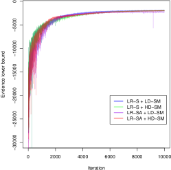
Figure 1: ${\cal L}(\lambda)$ for the variational approximations for the spatio-temporal example. The figure shows the estimated value of ${\cal L}(\lambda)$ vs iteration number for the four different parameterizations, see Section 5.3 or Table 1 for abbreviations.

Table 1: ${\cal L}(\lambda)$ and CPU time for the VB parameterizations in the spatio-temporal and Wishart process example. The table shows the estimated value of ${\cal L}(\lambda)$ for the different VB parameterizations by combining low-rank state / low-rank state and auxiliary (LR-S / LR-SA) with either of low-dimensional state mean / high-dimensional state mean (LD-SM / HD-SM). The estimate and its $95$% confidence interval are computed at the final iteration using $100$ Monte Carlo samples. The table also show the relative CPU (R-CPU) times, where the reference is LD-SM.

parameterization
Spatio-temporal		R-CPU		$\mathcal{L}(\lambda_{\mathrm{opt}})$		Confidence interval
LR-S + LD-SM		$1$		$\textnormal{-}1,996$		$[\textnormal{-}2,004;\textnormal{-}1,988]$
LR-S + HD-SM		$1.005$		$\textnormal{-}2,024$		$[\textnormal{-}2,032;\textnormal{-}2,016]$
LR-SA + LD-SM		$3.189$		$\textnormal{-}2,158$		$[\textnormal{-}2,167;\textnormal{-}2,148]$
LR-SA + HD-SM		$3.017$		$\textnormal{-}1,909$		$[\textnormal{-}1,918;\textnormal{-}1,900]$
Wishart process
LR-S + LD-SM		$1$		$\textnormal{-}1,121$		$[\textnormal{-}1,126;\textnormal{-}1,115]$
LR-S + HD-SM		$1.0004$		$\textnormal{-}1,040$		$[\textnormal{-}1,046;\textnormal{-}1,035]$

5.4 MCMC settings

Before comparing VB to MCMC, it is necessary to determine a reasonable burn-in period and number of iterations for inference for the Gibbs sampler in Wikle and Hooten,. It is clear that it is infeasible to monitor convergence for every single parameter in such a large scale model as (15), and therefore we focus on $\psi$, $u_{18}$ and $v_{19}$, which are among the variables considered in the analysis in Section 5.5.

Wikle and Hooten, use $50,000$ iterations of which $20,000$ are discarded as burn-in. We generate $4$ sampling chains with these settings and inspect convergence using the $\mathtt{coda}$ package (Plummer et al.,, 2006) in $\mathtt{R}$. We compute the Scale Reduction Factors (SRF) (Gelman and Rubin,, 1992) for $\psi,u_{18}$ and $v_{19}$ as a function of the number of Gibbs iterations. The adequate number of iterations in MCMC depends on what functionals of the parameters are of interest; here we monitor convergence for these quantities since we report marginal posterior distributions for these quantities later. The scale reduction factor of a parameter measures if there is a significant difference between the variance within the four chains and the variance between the four chains of that parameter. We use the rule of thumb that concludes convergence when $\mathrm{SRF}<1.1$, which gives a burn-in period of approximately $40,000$ here, for these functionals. After discarding these samples and applying a thinning of $10$ we are left with $1,000$ posterior samples for inference. However, as the draws are auto-correlated, this does not correspond to $1,000$ independent draws used in the analysis in Section 5.5 (note that we obtain independent samples from our variational posterior). To decide how many Gibbs samples are equivalent to $1,000$ independent samples for $\psi,u_{18}$ and $v_{19}$, we compute the Effective Sample Size (ESS) which takes into account the auto-correlation of the samples. We find that the smallest is $\mathrm{ESS}=5$ and hence we require $200,000$ iterations after a thinning of $10$, which makes a total of $2,000,000$ Gibbs iterations, excluding the burn-in of $40,000$. Thinning is advisable here due to memory issues — it is impractical to store $2,000,000$ iterations for each parameter (which may be used, for example, to estimate kernel densities) in high-dimensional models.

5.5 Analysis and results

We first consider inference on the diffusion coefficient $\psi_{i}$ for location $i$. Figure 2 shows the “true” posterior (represented by MCMC) together with the variational approximation for six locations described in the caption of the figure. The figure shows that the posterior distribution is highly skewed for locations with zero dove counts and approaches normality as the dove counts increase. Consequently, the accuracy of the variational posterior (which is Gaussian) improves with increasing dove counts. The figure also shows the phenomena we described in the beginning of Section 1: there is a discrepancy between the posterior densities. However, as we will see, it affects neither the location estimates of the intensity of the process nor its prediction.

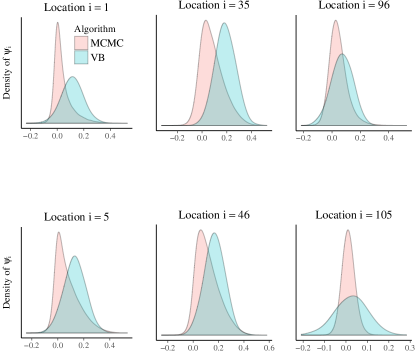
Figure 2: Distribution of the diffusion coefficients. The figure shows the posterior distribution of $\psi_{i}$ obtained by MCMC and VB. The locations are divided into three categories (total doves over time within brackets): zero count locations (Idaho, $i=1\,[0]$ , Arizona $i=5\,[0]$, left panels), low count locations (Texas, $i=35\,[16],46\,[21]$, middle panels) and high count locations (Florida, $i=96\,[1,566],105\,[1,453]$, right panels).

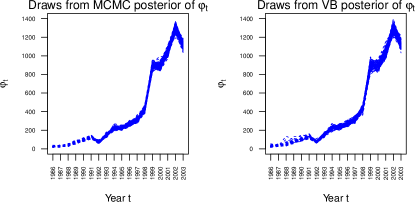
Figure 3: Samples from the posterior sum of dove intensity over the spatial grid for each year. The figure shows $100$ samples from the posterior distribution of $\varphi_{t}=\sum_{i}\exp(v_{it})$ obtained by MCMC (left panel) and VB (right panel).

Figure 3 shows 100 VB and MCMC posterior samples of the dove intensity for each year summed over the spatial locations, i.e. $\varphi_{t}=\sum_{i}\exp(v_{it})$. The two posteriors are similar and show an exponential increase of doves until the year $2002$ followed by a steep decline for $2003$.

Figure 4 summarises some spatial properties of the model. It shows a heat map of the MCMC and VB posterior means of the dove intensity $\varphi_{it}=\exp(v_{it})$ for the last five years of the data, overlaid on a map of the U.S. The figure confirms that VB gives accurate location estimates of the spatial process in this example.

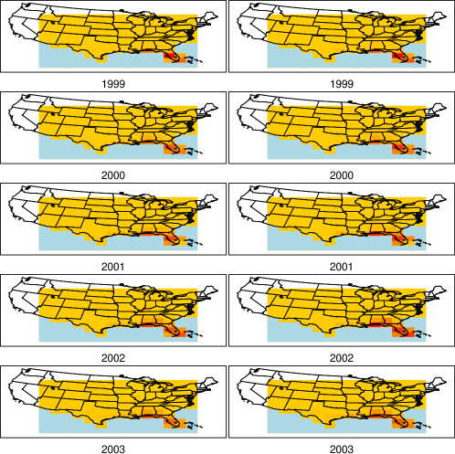
Figure 4: Posterior dove intensity for the years 1999-2003. The figure shows the posterior mean of $\varphi_{it}=\exp(v_{it})$ computed by MCMC (left panels) and VB (right panels) for $i=1,\dots,p=111,$ and the last $5$ years of the data ($t=14,15,16,17,18$). The results are illustrated with a spatial grid plotted together with a map of the United States, where the colors vary between low intensity (yellow) and high intensity (red). The light blue color is for aesthetic reasons and does not correspond to observed locations.

We draw the following conclusions from the analysis using the MCMC and VB posteriors, which are nearly identical. First, Figure 4 shows that the the dove intensity is most pronounced in the South East states, in particular Florida. Second, Figure 4 also shows that it is likely that the decline of doves for year $2003$ in Figure 3 can be attributed to a drop in the intensity at two areas of Florida: Central Florida ($i=96$) and South East Florida ($i=105$). Figure 5 illustrates the whole posterior distribution of the log-intensity for these locations at the year $2003$, as well as an out-of-sample posterior predictive distribution for year $2004$. Both estimates are kernel density estimates using approximately $1,000$ effective samples. The posterior distributions for the VB and MCMC are similar, and it is evident that using this large scale model for forecasting future values is associated with a large uncertainty.

Figure 6 illustrates the spatial basis functions and their reweighting over time to produce mean of the variational approximation, as discussed in Section 4.3.

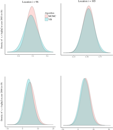
Figure 5: Forecasting the log-intensity of the spatial process. The figure shows an in-sample forecast density of the log-intensity $v_{it}$ for year 2003 ($t=18$, upper panels) and out-of-sample forecast density for year 2004 ($t=19$, lower panels) for Central Florida ($i=96$, left panels) and South East Florida ($i=105$, right panels).

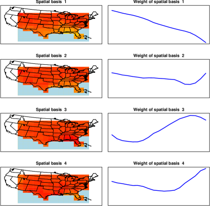
Figure 6: Spatial basis representation of the state vector. The figure shows the Spatial basis functions (left panel), i.e. the $j$th column of $B$, $j=1,\dots,q=4$ and the corresponding weights $\mu_{t}$ (right panel) through $t=0,\dots,18$, that fors $E(X_{t})=B\mu_{t}$.

6 Application 2: Stochastic volatility modeling

6.1 Model

The second example considers the Wishart based multivariate stochastic volatility model proposed in Philipov and Glickman, 2006b who used it to model the time-varying dependence of a portfolio of $k$ assets over $T$ time periods. Section 4.2 briefly discussed this model.

Philipov and Glickman, 2006b assume that the return at time period $t$, $t=1,\dots,T$, is the vector $y_{t}=(y_{t1},\dots,y_{tk})^{\top}$, with

$$y_{t} \sim \mathcal{N}(0,\Sigma_{t});\quad\Sigma_{t}\in\mathbb{R}^{p\times p};$$

$$\Sigma_{t}^{-1} \sim \mathrm{Wishart}(\nu,S_{t-1});\quad S_{t}=\frac{1}{\nu}H(\Sigma_{t}^{-1})^{d}H^{\top};\,S_{t}\in\mathbb{R}^{p\times p};\,\nu>k;\,0<d<1;$$

$H$ is a lower triangular Cholesky factor of a positive definite matrix $A$, with $A=HH^{\top}\in\mathbb{R}^{p\times p}$; and $\Sigma_{0}$ is assumed known. The prior for $A$ is inverse Wishart, i.e. $A^{-1}\sim\mathrm{Wishart}(\gamma_{0},Q_{0})$, with $\gamma_{0}=k+1$ and $Q_{0}=I$; a uniform prior on $[0,1]$ for $d$, i.e. $d\sim U[0,1]$; and a shifted gamma prior for $\nu$, i.e. $\nu-k\sim\mathrm{Gamma}(\alpha_{0},\beta_{0})$. The joint posterior density for $(\Sigma,A,\nu-k,d)$ is

$$p(\Sigma,A,\nu-k,d|y) \propto p(A,d,\nu-k)\prod_{t=1}^{T}p(\Sigma_{t}|\nu,S_{t-1})p(y_{t}|\Sigma_{t});$$ (16)

$p(A,d,\nu-k)$ is the joint prior density for $(A,d,\nu-k)$; $p(\Sigma_{t}|\nu,S_{t-1},d)$ is the conditional inverse Wishart prior for $\Sigma_{t}$ given $\nu$, $S_{t-1}$; and $d$, and $p(y_{t}|\Sigma_{t})$ is the normal density for $y_{t}$ given $\Sigma_{t}$.

We write $C_{t}$ for the Cholesky factor of $\Sigma_{t}$ and we reparameterize the posterior in terms of the unconstrained parameter vector

$$\theta=(\mathrm{vech}(H^{\prime})^{\top},d^{\prime},\nu^{\prime},\mathrm{vech}(C_{1}^{\prime})^{\top},\dots,\mathrm{vech}(C_{T}^{\prime})^{\top})^{\top};$$

where

$$C_{t}^{\prime}\in\mathbb{R}^{k\times k}; C^{\prime}_{t,ij}=C_{t,ij};\,i\neq j,\text{ and }C^{\prime}_{t,ii}=\log C_{t,ii};$$

$$H^{\prime}\in\mathbb{R}^{k\times k}; H^{\prime}_{ij}=H_{ij};\,i\neq j,\text{ and }H_{ii}=\log H_{ii};$$

with $d^{\prime}=\log d/(1-d)$ and $\nu^{\prime}=\log(\nu-k)$. Section S3.3 shows that

$$p(\theta|y)\propto |L_{k}(I_{k^{2}}+K_{k,k})(H\otimes I_{k})L_{k}^{\top}|\times\left\{\prod_{t=1}^{T}|L_{k}(I_{k^{2}}+K_{k,k})(C_{t}\otimes I_{k})L_{k}^{\top}|\right\}\times(\nu-k)$$ (17)

$$\times d(1-d)\times\left\{\prod_{i}H_{ii}\right\}\left\{\prod_{t=1}^{T}\prod_{i=1}^{k}C_{t,ii}\right\}\times p(A,d,\nu-k)\left\{\prod_{t=1}^{T}p(\Sigma_{t}|\nu,S_{t-1},d)p(y_{t}|\Sigma_{t})\right\};$$

Section S1 of the supplement defines the elimination matrix $L_{k}$ and the commutation matrix $K_{k,k}$; Section S3.4 of the supplement shows how to evaluate the gradient of the log posterior.

6.2 Evaluating the predictive performance of the variational approximation

Philipov and Glickman, 2006b develop an MCMC algorithm to estimate their Wishart based multivariate stochastic volatility model. Rinnergschwentner et al., (2012) point out that the Gibbs sampler developed by Philipov and Glickman, 2006b contains a mistake which affects all the full conditionals. We find that implementing the ‘corrected’ version of their algorithm results in a very inefficient sampler even for the $k=5$ portfolios used by Philipov and Glickman, 2006b in their empirical example. This means that the ‘corrected’ Philipov and Glickman, 2006b algorithm cannot be used as a ‘gold standard’ to compare against the variational approximation results. Although it may be possible to estimate the posterior of Philipov and Glickman, 2006b’s model using particle methods, we do not pursue this here. Section S7 of the supplement illustrates the inefficiency of the corrected Philipov and Glickman, 2006b sampler and explains its problems.

We now show empirically (by simulation) that the variational posterior provides useful predictive inference. Since MCMC is unavailable, the GVA is benchmarked against an oracle predictive approach, which assumes the the static model parameters are known. We use a bootstrap particle filter (Gordon et al.,, 1993) to obtain the posterior density of the state-vector at $t=T$; it is then possible to obtain the one-step ahead oracle predictive density $p(y_{T+1}|y_{1:T},\zeta^{\mathrm{true}})$, where $\zeta^{\mathrm{true}}$ denotes the true static model parameters. The variational predictive density is then benchmarked against the oracle predictive density; we note that the variational predictive density integrates over the variational posterior of all the parameters, including the static model parameters.

Section S5.1 of the supplement shows how to simulate from the oracle predictive density. Section S5.2 of the supplement shows how to simulate from the variational predictive density. The one-step ahead prediction is repeated for $H=4$ horizons. At horizons $h=1,\dots,H$, both filtering densities are based on $y_{1:T+h-1}$ and the optimization for finding the variational posterior for $h>1$ is fast since the variational parameters are initialized (except the ones added at $T+h$) at their variational mode from the previous optimization.

6.3 Variational approximations of the posterior distribution

Since this example does not include a high-dimensional auxiliary variable, we use the low-rank state (LR-S) parameterization combined with both a low-dimensional state mean (LD-SM) and a high-dimensional state mean (HD-SM). As in the previous example, it is straightforward to deduce conditional independence relationships in (17) to build the Cholesky factor $C_{2}$ of the precision matrix $\Omega_{2}$ of $\zeta$ in Section 4; this section also outlines how to construct the Cholesky factor $C_{1}$ of the precision matrix $\Omega_{1}$ of $z$. Massive parsimony is achieved in this application. In particular, for $k=12$ assets, the saturated Gaussian variational approximation has $31,059,020$ parameters, while our parameterization has $10,813$. For $k=5$, the saturated case has $1,152,920$ parameters and our parameterizations has $4,009\text{-}5,109$. See Section S6 of the supplement for more details.

For all variational approximations we let $q=4$ and perform $10,000$ iterations of a stochastic optimization algorithm with learning rates chosen adaptively according to the ADADELTA approach (Zeiler,, 2012). We initialize $B$ and $C$ as unit diagonals and choose $\mu$ and $D$ randomly. Figure 7 monitors the estimated ELBO for both parameterizations, using both the gradient estimators in Roeder et al., and the alternative standard ones which do not cancel terms that have zero expectation. For $k=5$, the figure shows that the different gradient estimators perform equally well. Moreover, slightly more variable estimates are observed in the beginning for the low-dimensional state mean parameterization compared to that of the high-dimensional mean. Table 1 presents estimates of ${\cal L}(\lambda)$ at the final iteration using $100$ Monte Carlo samples and also presents the relative CPU times of the algorithms. In this example, the separate state mean present in the high-dimensional state mean seems to improve the ELBO considerably.

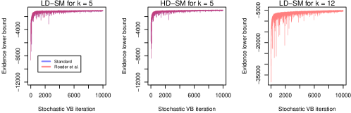
Figure 7: ${\cal L}(\lambda)$ for the variational approximations in the Wishart process example. The figure shows the estimated value of ${\cal L}(\lambda)$ vs iteration number using a low-dimensional state mean / high-dimensional state mean (LD-SM / HD-SM) with the gradient estimator in Roeder et al., (2017) or the standard estimator. The left and middle panels are for $k=5$; the right panel is for the real data with $k=12$.

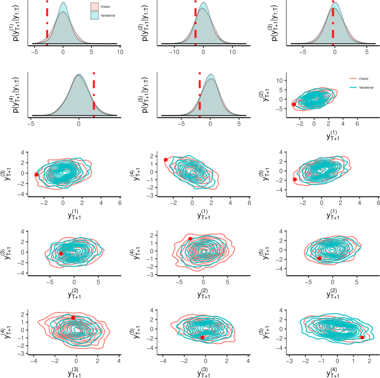
Figure 8: Multivariate stochastic volatility model with simulated data and $T=100$. The top row and the two panels from the left of the second row show the marginal one-step-ahead kernel density estimates of the predictive density for each of the $k=5$ variables for both the variational approximation and the oracle; the test observation is the red line. The right panel of the second row and the rest of the panels show the contour plots of the kernel density estimates of the one-step-ahead bivariate predictive densities for the variational approximation and the oracle; the red dot is the test observation.

6.4 Results for simulated data

We now assess the variational approximation by comparing its out-of-sample predictive properties against the oracle predictive density. See Section 6.2. The comparison is based on data generated by the multivariate stochastic volatility model with $d=0.2$, $\nu=20$ and $A$ generated from $\sim\mathrm{Inv\textnormal{-}Wishart}(5,\mathrm{diag}(5))$. While the reported results are for a particular simulated dataset due to space restrictions, we have verified that the same performance is obtained when the random number seed is changed and $d$ and $\nu$ are varied. Figure 8 shows the kernel density estimates for the marginals of all five parameters and bivariate kernel density estimates for all pairs of variables for the predictive $p(y_{T+1}|y_{1:T})$ (variational and oracle) for $T=100$. The figure also shows the test observation (withheld when estimating the variational predictive and the oracle predictive). Figure 9 shows boxplots of draws from all marginals of the predictive densities $p(y_{T+h}|y_{1:T+h-1})$ (variational and oracle) for the horizons $h=1,2,3,4$. This figure also shows the withheld test observation which is within the prediction intervals of both methods. Figure 10 shows, for each of the $H=4$ horizons, future predictions (variational and oracle) of an equally weighted portfolio $w_{T+h}=\sum_{k=1}^{5}(1/5)y_{(T+h)k}$ conditional on the posteriors using the data $y_{1:(T+h-1)}$. Section S5.3 of the supplement gives more plots that further confirm the accuracy of the variational predictive densities.

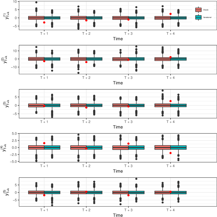
Figure 9: Simulated data. Boxplots of samples from the variational one-step ahead marginal predictive densities compared against the oracle predictive densities with $T=100,101,102,103$. The figure also shows the test observation (red) dot for each $T$ and variable.

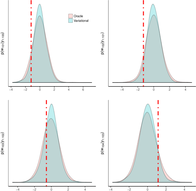
Figure 10: Simulated data. Kernel density estimates of the one-step ahead predictive densities of a equally weighted portfolio of assets. The results are for $T=100,101,102,103$. The figure also shows the test observation (red line) for each $T$.

6.5 Real data results

The data consists of $T=100$ monthly observations on all $k=12$ (Philipov and Glickman, 2006b only consider $k=5$ assets and report an acceptance probability close to zero when $k=12$ for their sampler) value-weighted portfolios from the 201709 CRSP database, for the period 2009-06 to 2017-09. The portfolios are: consumer non-durables, consumer durables, manufacturing, energy, chemicals, business equipment, telecom, utilities, retail/wholesale, health care, finance, other. With $k=12$ the dimension of the state vector is $p=78$. We follow Philipov and Glickman, 2006b and prefilter each series using an AR(1) process.

The right panel in Figure 7 shows the estimated ELBO on a variational optimization using the real dataset. While the estimated ELBO plot is more variable than for the $k=5$ case, it settles down eventually. Figure 11 shows the in-sample prediction of $\tilde{y}_{100}$ given $y_{1:100}$, together with the observed data point, for some of the assets. The figure also shows an in-sample prediction of a portfolio consisting of equally weighted assets. The variational posterior for the real data example uses the low-dimensional state mean parameterization.

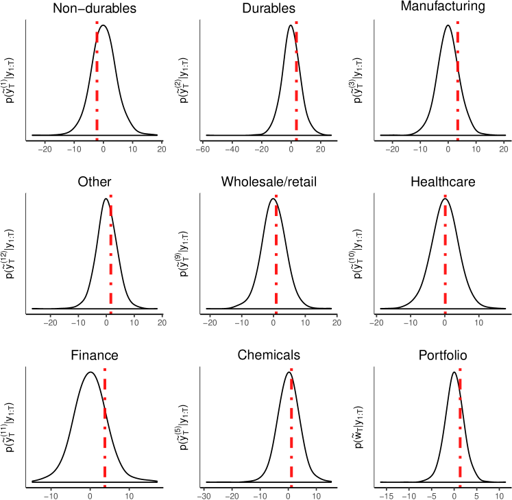
Figure 11: Multivariate stochastic volatility model: Real data. Kernel density estimates of the in-sample predictive density for some the assets and a equally weighted portfolio of assets. The figure also shows the in-sample observation (red line).

7 Discussion

The article proposes a Gaussian variational approximation method for high-dimensional state space models. Dimension reduction in the variational approximation is achieved through a dynamic factor structure for the variational covariance matrix. The factor structure reduces the dimension in the description of the states, whereas the Markov dynamic structure for the factors achieves parsimony in describing the temporal dependence. We show that the method works well in two challenging models. The first is an extended example for a spatio-temporal data set describing the spread of the Eurasian collared-dove throughout North America. The second is a multivariate stochastic volatility model in which the state vector is high dimensional.

Perhaps the most obvious limitation of our current work is the restriction to a Gaussian approximation, which does not allow capturing skewness or heavy tails in the posterior distribution. However, Gaussian variational approximations can be used as building blocks for more complex approximations based on normal mixtures, copulas or conditionally Gaussian families for example (Han et al.,, 2016; Miller et al.,, 2017; Smith et al.,, 2019; Tan et al.,, 2019) and these more complex variational families can overcome some of the limitations of the simple Gaussian approximation. We intend to consider this in future work.

Appendix A Gradient expressions of the evidence lower bound

A.1 Notation and definitions

We consider any vector $x\in\mathbb{R}^{n}$ to be arranged as a column vector with $n$ elements, i.e. $x=(x_{1},\dots,x_{n})^{\top}$. Likewise, if $g$ is function whose output is vector valued, i.e. $g(x)\in\mathbb{R}^{m}$, then $g(x)=(g_{1}(x),\dots,g_{m}(x))^{\top}$. For a matrix $A$, $\mathrm{vec}(A)$ is the vector obtained by stacking the columns of $A$ from left to right.

Definition A1.

1. Suppose that $g:\mathbb{R}^{n}\to\mathbb{R}$ is a scalar valued function of a vector valued argument $x$. Then $\nabla_{x}g$ is a column vector with $i$th element $\partial g/\partial x_{i}$.

2. Suppose that $g:\mathbb{R}^{n}\to\mathbb{R}^{m}$ is a vector valued function of a vector valued argument $x$. Then $dg/dx$ is a $m\times n$ matrix with $(i,j)$th element $\mbox{$\partial g_{i}$}/\mbox{$\partial x_{j}$}$.

3. Suppose that $g:\mathbb{R}^{m\times n}\to\mathbb{R}$ is a scalar valued function of a $m\times n$ matrix $A=(a_{ij})$. Then $\nabla_{A}g$ is an $m\times n$ matrix with $(i,j)$th element $\mbox{$\partial g$}/\mbox{$\partial a_{ij}$}$.

4. Suppose that $G:\mathbb{R}^{m\times n}\to\mathbb{R}^{q\times r}$ is a matrix valued function of a matrix valued argument $A$. Then,

   $$\frac{dG}{dA}\coloneqq\frac{d\mathrm{vec}(G)}{d\mathrm{vec}(A)}$$

   is an $mq\times nr$ matrix with $(i,j)$th element $\mbox{$\partial\mathrm{vec}(G)_{i}$}/\mbox{$\partial\mathrm{vec}(A)_{j}$}$.

Remark A1.

If $g$ is a scalar function of a vector valued argument $x$, then Part (ii) (with $m=1$) implies that $dg/dx$ is a row vector. Hence, $\nabla_{X}g=(dg/dx)^{\top}$.

We write $0_{m\times n}$ for the $m\times n$ matrix of zeros, $\otimes$ for the Kronecker product and $\odot$ for the Hadmard (elementwise) product which can be applied to two matrices of the same dimensions. For an $m\times n$ matrix $A$, $\mathrm{vec}(A)$ is the vector obtained by stacking the columns of $A$ from left to right. We also write $K_{r,s}$ for the commutation matrix, of dimensions $rs\times rs$, which for an $r\times s$ matrix $Z$ satisfies

$$K_{r,s}\mathrm{vec}(Z)=\mathrm{vec}(Z^{\top}).$$

A.2 Results

We adopt the notation from Section 4.3 and construct the variational distribution for $\theta$ through

$$\theta =\left[\begin{array}[]{cc}X\\ \zeta\end{array}\right]=\left[\begin{array}[]{cc}I_{T+1}\otimes B&0\\ 0&I_{P}\end{array}\right]\rho+\left[\begin{array}[]{c}\epsilon\\ 0\end{array}\right];$$

$P=\dim(\zeta)$ and $\epsilon=(\epsilon_{0}^{\top},\dots,\epsilon_{T}^{\top})^{\top}$; $\epsilon_{t}$ is defined in (12). Apply the reparameterization trick for the LD-SM parameterization (see the discussion in Section 4.3) and write

$$\theta =W\mu+WC^{-\top}\omega+Ze;$$ (A1)

where $\omega\sim\mathcal{N}(0,I_{q(T+1)})$;

$$W=\left[\begin{array}[]{cc}I_{T+1}\otimes B&0_{p(T+1)\times P}\\ 0_{P\times q(T+1)}&I_{P}\end{array}\right],\;\;\;\;Z=\left[\begin{array}[]{cc}D&0_{p(T+1)\times P}\\ 0_{P\times p(T+1)}&0_{P\times P}\end{array}\right],\;\;\;\;e=\left[\begin{array}[]{c}\epsilon\\ 0_{P\times 1}\end{array}\right];$$

and $D$ is a diagonal matrix with diagonal entries $(\delta_{0}^{\top},\dots,\delta_{T}^{\top})^{\top}$. Then, the distribution of $(\omega,\epsilon)\sim\mathcal{N}(0,I_{(p+q)(T+1)+P})$ does not depend on the variational parameter $\lambda$.

Lemmas A1 and A2 give the gradients of the ELBO in (5) using the reparameterization trick. These can be used for unbiased gradient estimation of the lower bound by sampling one or more samples from $(\omega,\epsilon)$. Lemma A1 (A2) contains the gradients corresponding to (6) ((7)), which we refer to as the standard gradient (the Roeder et al., gradient). By the discussion in Section 2, the Roeder et al., gradient has the property that a Monte Carlo estimate of the gradient based on (A6) using a single sample is zero when the variational posterior is exact. The proofs of the lemmas are in Section S3.1 of the supplement.

Lemma A1 (Standard gradient).

Let $\mathcal{L}(\lambda)=E_{(\omega,\epsilon)}\left(\log h(\theta)-\log q_{\lambda}(\theta)\right),$ with $\theta$ in (A1), $(\omega,\epsilon)$ as above, and $q_{\lambda}(\theta)=\mathcal{N}\left(\theta|W\mu,W\Sigma W^{\top}+Z^{2}\right).$ If $h(\theta)$ is differentiable, then,

1. $$\nabla_{\mu}{\cal L}(\lambda) =W^{\top}E_{(\omega,\epsilon)}(\nabla_{\theta}\log h(W\mu+WC^{-\top}\omega+Ze));$$ (A2)

2. $$\nabla_{\mathrm{vec}(B)}{\cal L}(\lambda) =T_{1B}+T_{2B}+T_{3B},$$ (A3)

   where

   $$T_{1B} =\left\{\frac{dW}{dB}\right\}^{\top}E_{(\omega,\epsilon)}(((\mu+C^{-\top}\omega)\otimes I_{p(T+1)+P})\nabla_{\theta}\log h(W\mu+WC^{-\top}\omega+Ze)),$$

   $$T_{2B} =\left\{\frac{dW}{dB}\right\}^{\top}\mathrm{vec}((W\Sigma W^{\top}+Z^{2})^{-1}W\Sigma),$$

   $$T_{3B} =\left\{\frac{dW}{dB}\right\}^{\top}E_{(\omega,\epsilon)}\left(\mathrm{vec}\left((W\Sigma W^{\top}+Z^{2})^{-1}(WC^{-\top}\omega+Ze)\omega^{\top}C^{-1}\right.\right.$$

   $$\left.\left.-(W\Sigma W^{\top}+Z^{2})^{-1}(WC^{-\top}\omega+Ze)(WC^{-\top}\omega+Ze)^{\top}(W\Sigma W^{\top}+Z^{2})^{-1}W\Sigma\right)\right);$$

   above,

   $$\frac{dW}{dB}= (Q_{1}^{\top}\otimes P_{1})\left[\left\{(I_{T+1}\otimes K_{q,(T+1)})(\mbox{$\mathrm{vec}(I_{T+1})$}\otimes I_{q})\right\}\otimes I_{p}\right],$$

   with

   $$P_{1}=\left[\begin{array}[]{c}I_{p(T+1)}\\ 0_{P\times p(T+1)}\end{array}\right],\;\;\;\;Q_{1}=\left[\begin{array}[]{cc}I_{q(T+1)}&0_{q(T+1)\times P}\end{array}\right];$$

3. $$\nabla_{\delta}{\cal L}(\lambda) =E_{(\omega,\epsilon)}(\mathrm{diag}(\nabla_{X}\log h(W\mu+WC^{-\top}\omega+Ze)\epsilon^{\top}+(W_{1}\Sigma_{1}W_{1}^{\top}+D^{2})^{-1}D$$

   $$+(W_{1}\Sigma_{1}W_{1}^{\top}+D^{2})^{-1}(W_{1}C_{1}^{-\top}\omega_{1}+D\epsilon)\epsilon^{\top}$$

   $$-(W_{1}\Sigma_{1}W_{1}^{\top}+D^{2})^{-1}(W_{1}C_{1}^{-\top}\omega_{1}+D\epsilon)(W_{1}C_{1}^{-\top}\omega_{1}+D\epsilon)^{\top}(W_{1}\Sigma_{1}W_{1}^{\top}+D^{2})^{-1}D)),$$ (A4)

   where $W_{1}=I_{T+1}\otimes B$;

4. $$\nabla_{C}{\cal L}(\lambda)= E_{(\omega,\epsilon)}\left(-C^{-\top}\omega\nabla_{\theta}\log h(W\mu+WC^{-\top}\omega+Ze)^{\top}WC^{-\top}\right.$$

   $$- \Sigma W^{\top}(W\Sigma W^{\top}+Z^{2})^{-1}WC^{-\top}$$

   $$- C^{-\top}\omega(WC^{-\top}\omega+Ze)^{\top}(W\Sigma W^{\top}+Z^{2})^{-1}WC^{-\top}$$

   $$+ \left.\Sigma W^{\top}(W\Sigma W^{\top}+Z^{2})^{-1}(WC^{-\top}\omega+Ze)(WC^{-\top}\omega+Ze)^{\top}(W\Sigma W^{\top}+Z^{2})^{-1}WC^{-\top}\right)$$ (A5)

Lemma A2 (Roeder et al., gradient).

Let $\mathcal{L}(\lambda)=E_{(\omega,\epsilon)}\left(\log h(\theta)-\log q_{\lambda}(\theta)\right)$, with $\theta$ defined in (A1), ${(\omega,\epsilon)}$ as above and $q_{\lambda}(\theta)=\mathcal{N}\left(\theta|W\mu,W\Sigma W^{\top}+Z^{2}\right).$

If $h(\theta)$ is differentiable, then

1. $$\nabla_{\mu}{\cal L}(\lambda) =W^{\top}E_{(\omega,\epsilon)}(\nabla_{\theta}\log h(W\mu+WC^{-\top}\omega+Ze)+(W\Sigma W^{\top}+Z^{2})^{-1}(WC^{-\top}\omega+Ze));$$ (A6)

2. $$\nabla_{\mathrm{vec}(B)}{\cal L}(\lambda) =T_{1B}+T_{3B}^{\prime},$$ (A7)

   with $T_{1B}$ as in Part (ii) of Lemma A1 and

   $$T_{3B}^{\prime} =\left\{\frac{dW}{dB}\right\}^{\top}E_{(\omega,\epsilon)}\left(\mathrm{vec}\left((W\Sigma W^{\top}+Z^{2})^{-1}(WC^{-\top}\omega+Ze)(\omega^{\top}C^{-1}+\mu^{\top})\right)\right);$$ (A8)

3. $$\nabla_{\delta}{\cal L}(\lambda) =E_{(\omega,\epsilon)}(\mathrm{diag}(\nabla_{X}\log h(W\mu+WC^{-\top}\omega+Ze)\epsilon^{\top}$$

   $$+(W_{1}\Sigma_{1}W_{1}^{\top}+D^{2})^{-1}(W_{1}C_{1}^{-\top}\omega_{1}+D\epsilon)\epsilon^{\top})),$$ (A9)

   where $W_{1}=I_{T+1}\otimes B$;

4. $$\nabla_{C}{\cal L}(\lambda)= E_{(\omega,\epsilon)}\left(-C^{-\top}\omega\left\{\nabla_{\theta}\log h(W\mu+WC^{-\top}\omega+Ze)^{\top}\right.\right.$$

   $$+ \left.\left.(WC^{-\top}\omega+Ze)^{\top}(W\Sigma W^{\top}+Z^{2})^{-1}\right\}WC^{-\top}\right).$$ (A10)

Online supplement to ‘Gaussian variational approximations for high-dimensional state-space models’.

We refer to equations, sections, etc in the main paper as (1), Section 1, etc, and in the supplement as (S1), Section S1, etc.

S1 Notation and definitions

To make the supplement easier to follow we repeat some of the material in Appendix A and add to it the new notation needed in this supplement. We consider any $n$ dimensional $x$ to be a column vector, i.e. $x=(x_{1},\dots,x_{n})^{\top}$; thus, if $g$ is function whose output is $m$ dimensional, then $g(x)=(g_{1}(x),\dots,g_{m}(x))^{\top}$. For a matrix $A$, $\mathrm{vec}(A)$ is the vector obtained by stacking the columns of $A$ from left to right.

Definition S2.

1. Suppose that $g:\mathbb{R}^{n}\to\mathbb{R}$ is a scalar valued function of a vector valued argument $x$. Then $\nabla_{x}g$ is a column vector with $i$th element $\partial g/\partial x_{i}$.

2. Suppose that $g:\mathbb{R}^{n}\to\mathbb{R}^{m}$ is a vector valued function of a vector valued argument $x$. Then $dg/dx$ is a $m\times n$ matrix with $(i,j)$th element $\mbox{$\partial g_{i}$}/\mbox{$\partial x_{j}$}$.

3. Suppose that $g:\mathbb{R}^{m\times n}\to\mathbb{R}$ is a scalar valued function of a $m\times n$ matrix $A=(a_{ij})$. Then $\nabla_{A}g$ is an $m\times n$ matrix with $(i,j)$th element $\mbox{$\partial g$}/\mbox{$\partial a_{ij}$}$.

4. Suppose that $G:\mathbb{R}^{m\times n}\to\mathbb{R}^{q\times r}$ is a matrix valued function of a matrix valued argument $A$. Then,

   $$\frac{dG}{dA}\coloneqq\frac{d\mathrm{vec}(G)}{d\mathrm{vec}(A)}$$

   is an $mq\times nr$ matrix with $(i,j)$th element $\mbox{$\partial\mathrm{vec}(G)_{i}$}/\mbox{$\partial\mathrm{vec}(A)_{j}$}$.

Remark S2.

If $g$ is a scalar function of a vector valued argument $x$, then Part (ii) (with $m=1$) implies that $dg/dx$ is a row vector. Hence, $\nabla_{X}g=(dg/dx)^{\top}$.

Remark S3.

Part (iv), with $r=1$, covers the case of the derivative of a vector valued function with respect to a matrix valued argument.

Let $0_{m\times n}$ be the $m\times n$ matrix of zeros; let $\otimes$ be the Kronecker product and $\odot$ the Hadmard (elementwise) product, both of which can be applied to two matrices of the same dimensions. For a $n\times n$ symmetric matrix $A$, $\mathrm{vech}(A)$ is the column vector of length $n(n+1)/2$ obtained by vectorizing the lower triangular and diagonal parts of $A$; the $L_{n}$ elimination matrix is defined by $\mathrm{vech}(A)=:L_{k}\mathrm{vec}(A)$; and the duplication matrix $D_{n}$ is defined by $\mathrm{vec}(A)=:D_{k}\mathrm{vech}(A)$; see Magnus and Neudecker, (1980) for further properties of the elimination and duplication matrices. We also write $K_{r,s}$ for the commutation matrix of dimensions $rs\times rs$, which for an $r\times s$ matrix $Z$ satisfies

$$K_{r,s}\mathrm{vec}(Z)=\mathrm{vec}(Z^{\top}).$$

S2 Details on the sparsity of the precision matrix of the dynamic factors

Write $\Sigma_{1}$ for the covariance matrix of the latent dynamic factors $z=(z_{0}^{\top},\dots,z_{T}^{\top})^{\top}$ and let $\Omega_{1}=\Sigma^{-1}_{1}$ be the corresponding precision matrix. Denote by $C_{1}$ the lower triangular Cholesky factor of $\Omega_{1}$, i.e. $\Omega_{1}=C_{1}C^{\top}_{1}$. Section 4.3 assumes that $C_{1}$ takes the form

$$C_{1} =\begin{bmatrix}C_{00}&0&0&\ldots&0&0\\ C_{10}&C_{11}&0&\ldots&0&0\\ 0&C_{21}&C_{22}&\ldots&0&0\\ \vdots&\vdots&\vdots&\ddots&\vdots&\vdots\\ 0&0&0&\ldots&C_{T-1,T-1}&0\\ 0&0&\ldots&\ldots&C_{T,T-1}&C_{TT}\end{bmatrix},$$ (S1)

where the blocks in this block partitioned matrix follow the blocks of $z$; the corresponding precision matrix takes the form

$$\Omega_{1} =\begin{bmatrix}\Omega_{00}&\Omega_{10}^{\top}&0&\ldots&0&0\\ \Omega_{10}&\Omega_{11}&\Omega_{21}^{\top}&\ldots&0&0\\ 0&\Omega_{21}&\Omega_{22}&\ldots&0&0\\ \vdots&\vdots&\vdots&\ddots&\ldots&\vdots&\\ 0&0&0&\ldots&\Omega_{T-1,T-1}&\Omega_{T,T-1}^{\top}\\ 0&0&0&\ldots&\Omega_{T,T-1}&\Omega_{TT}\\ \end{bmatrix}.$$ (S2)

S3 Derivations

S3.1 Gradients of the variational approximation

This section proves Lemmas A1 and A2, which contain the gradient with respect to the variational parameters when applying the reparameterization trick as outlined in Section 4.3. The following result about the $\mathrm{vec}$ and Kronecker product is useful. For conformably dimensioned matrices $A$, $B$ and $C$,

$$\mathrm{vec}(ABC) =(C^{\top}\otimes A)\mathrm{vec}(B).$$

Using the notation in Section 4 and Appendix A, $\theta\sim q_{\lambda}(\theta)$, and its generative form is given by $\theta=W\mu+WC^{-\top}\omega+Ze$; thus,

$$\log q_{\lambda}(\theta)= -\frac{p(T+1)+P}{2}\log 2\pi-\frac{1}{2}\log|W\Sigma W^{\top}+Z^{2}|$$

$$-\frac{1}{2}(WC^{-\top}\omega+Ze)^{\top}(W\Sigma W^{\top}+Z^{2})^{-1}(WC^{-\top}\omega+Ze).$$ (S3)

Proof of Lemma A1.

Proof of Part (i). Since (S3) does not depend on $\mu$,

$$\nabla_{\mu}{\cal L}(\lambda)= \nabla_{\mu}E_{(\omega,\epsilon)}(\log h(W\mu+WC^{-\top}\omega+Ze))$$

$$= E_{(\omega,\epsilon)}(W^{\top}\nabla_{\theta}\log h(W\mu+WC^{-\top}\omega+Ze)).$$

Proof of Part (ii). For the parametrization outlined in Section 3.3, we use the derivations in Ong et al., (2018),

$$\nabla_{\mbox{vec$(B)$}}E_{(\omega,\epsilon)}\left(\frac{1}{2}\log|BB^{\top}+D^{2}|\right)= \mathrm{vec}((BB^{\top}+D^{2})^{-1}B),$$ (S4)

$$\nabla_{B}E_{(\omega,\epsilon)}\Bigl{(}-\frac{1}{2}\mbox{tr}((B\omega+\delta\odot\kappa)^{\top} (BB^{\top}+D^{2})^{-1}(B\omega+\delta\odot\kappa))\Bigr{)}=E_{(\omega,\epsilon)}(-(BB^{\top}+D^{2})^{-1}(B\omega+\delta\odot\kappa)\omega^{\top}$$

$$+(BB^{\top}+D^{2})^{-1}(B\omega+\delta\odot\kappa)(B\delta+\delta\odot\kappa)^{\top}(BB^{\top}+D^{2})^{-1}B),$$ (S5)

$$\nabla_{\delta}{\cal L}(\lambda)= E_{(\omega,\epsilon)}(\mbox{diag}(\nabla_{\theta}h(\mu+B\omega+\delta\odot\kappa)\kappa^{\top}+(BB^{\top}+D^{2})^{-1}(B\omega+\delta\odot\kappa)\kappa^{\top}).$$ (S6)

In deriving an expression for $\nabla_{\mathrm{vec}(B)}{\cal L}(\lambda)$, it is helpful to have an explicit expression for $dW/dB$. We can write $W=W_{1}+W_{2}$, with $\mathrm{vec}(W)=\mathrm{vec}(W_{1})+\mathrm{vec}(W_{2})$; and

$$W_{1}=\left[\begin{array}[]{cc}I_{T+1}\otimes B&0_{p(T+1)\times P}\\ 0_{P\times q(T+1)}&0_{P\times P}\end{array}\right],\;\;\;\;W_{2}=\left[\begin{array}[]{cc}0_{p(T+1)\times q(T+1)}&0_{p(T+1)\times P}\\ 0_{P\times q(T+1)}&I_{P}\end{array}\right].$$

Using Theorem 1 of Caswell and van Daalen, (2016), $\mathrm{vec}(W_{1})=(Q_{1}^{\top}\otimes P_{1})\mathrm{vec}(I_{T+1}\otimes B)$; with

$$P_{1}=\left[\begin{array}[]{c}I_{p(T+1)}\\ 0_{P\times p(T+1)}\end{array}\right],\;\;\;\;Q_{1}=\left[\begin{array}[]{cc}I_{q(T+1)}&0_{q(T+1)\times P}\end{array}\right];$$

$\mathrm{vec}(W_{2})$ can be written similarly, but its expression is unnecessary since $W_{2}$ does not depend on $B$. Using standard results on the differentiation of Kronecker products,

$$\frac{dW}{dB}= (Q_{1}^{\top}\otimes P_{1})\frac{d(I_{T+1}\otimes B)}{dB},$$ (S7)

$$= (Q_{1}^{\top}\otimes P_{1})\left[\left\{(I_{T+1}\otimes K_{q,(T+1)})(\mbox{$\mathrm{vec}(I_{T+1})$}\otimes I_{q})\right\}\otimes I_{p}\right].$$ (S8)

Then,

$$\nabla_{\mathrm{vec}(B)}{\cal L}(\lambda)= T_{1B}+T_{2B}+T_{3B},$$

where

$$T_{1B}= E_{(\omega,\epsilon)}(\nabla_{\mathrm{vec}(B)}\log h(W\mu+WC^{-\top}\omega+Ze)),$$

$$=E_{(\omega,\epsilon)}\left(\left\{\frac{dW}{dB}\right\}^{\top}((\mu+C^{-\top}\omega)\otimes I_{p(T+1)+P})\nabla_{\theta}\log h(W\mu+WC^{-\top}\omega+Ze)\right);$$ (S9)

$$T_{2B}= \left\{\frac{dW}{dB}\right\}^{\top}\left\{\frac{dWC^{-\top}}{dW}\right\}^{\top}\nabla_{\mathrm{vec}(WC^{-\top})}\left\{\frac{1}{2}\log|WC^{-T}C^{-1}W^{\top}+Z^{2}|\right\}$$

$$= \left\{\frac{dW}{dB}\right\}^{\top}(C^{-\top}\otimes I_{p(T+1)+P})\mathrm{vec}((WC^{-\top}C^{-1}W^{\top}+Z^{2})^{-1}WC^{-\top})$$

$$= \left\{\frac{dW}{dB}\right\}^{\top}\mathrm{vec}((WC^{-\top}C^{-1}W^{\top}+Z^{2})^{-1}WC^{-\top}C^{-1}),$$ (S10)

using (S4); and using (S5)

$$T_{3B}= \nabla_{\mathrm{vec}(B)}E_{(\omega,\epsilon)}\left(\frac{1}{2}(WC^{-\top}\omega+Ze)^{\top}(W\Sigma W^{\top}+Z^{2})^{-1}(WC^{-\top}\omega+Ze)\right)$$

$$= \left\{\frac{dW}{dB}\right\}^{\top}\left\{\frac{dWC^{-\top}}{dW}\right\}^{\top}\nabla_{\mathrm{vec}(WC^{-\top})}E_{f}\left(\frac{1}{2}(WC^{-\top}\omega+Ze)^{\top}(W\Sigma W^{\top}+Z^{2})^{-1}\right.$$

$$\left.(WC^{-\top}\omega+Ze)\right)$$

$$= \left\{\frac{dW}{dB}\right\}^{\top}(C^{-\top}\otimes I_{p(T+1)+P})\mathrm{vec}\left(E_{f}\left\{(W\Sigma W^{\top}+Z^{2})^{-1}(WC^{-\top}\omega+Ze)\omega^{\top}\right.\right.$$

$$- \left.\left.(W\Sigma W^{\top}+Z^{2})^{-1}(WC^{-\top}\omega+Ze)(WC^{-\top}\omega+Ze)^{\top}(W\Sigma W^{\top}+Z^{2})^{-1}WC^{-\top}\right\}\right).$$ (S11)

Equation (A3) is obtained by combining (S9)– (S11).

Proof of Part (iii). The derivation of the gradient is identical to that of (S6), giving (A4) directly.

Proof of Part (iv). Writing

$$\nabla_{\mathrm{vec}(C)}{\cal L}(\lambda)= T_{1C}+T_{2C}+T_{3C},$$

where

$$T_{1C}= \nabla_{\mathrm{vec}(C)}E_{(\omega,\epsilon)}(\log h(W\mu+WC^{-\top}\omega+Ze))$$

$$= \left\{\frac{dC^{-1}}{dC}\right\}^{\top}\left\{\frac{dC^{-\top}}{dC^{-1}}\right\}^{\top}\left\{\frac{dWC^{-\top}\omega}{dWC^{-\top}}\right\}^{\top}E_{f}(\nabla_{\theta}\log h(W\mu+WC^{-\top}\omega+Ze))$$

$$= E_{(\omega,\epsilon)}\left(-(C^{-1}\otimes C^{-\top})K_{q(T+1)+P,q(T+1)+P}(I_{q(T+1)+P}\otimes W^{\top})(\omega\otimes I_{q(T+1)+P})\right.$$

$$\left.\nabla_{\theta}\log h(W\mu+WC^{-\top}\omega+Ze)\right)$$

$$= -E_{(\omega,\epsilon)}(\mathrm{vec}(C^{-\top}\omega\nabla_{\theta}\log h(W\mu+WC^{-\top}\omega+Ze)^{\top}WC^{-\top}));$$ (S12)

$$T_{2C}= \nabla_{\mathrm{vec}(C)}\frac{1}{2}\log|WC^{-\top}C^{-1}W^{\top}+Z^{2}|$$

$$= \left\{\frac{dC^{-1}}{dC}\right\}^{\top}\left\{\frac{dC^{-\top}}{dC^{-1}}\right\}^{\top}\left\{\frac{dWC^{-\top}}{dC^{-\top}}\right\}^{\top}\nabla_{\mathrm{vec}(WC^{-\top})}\frac{1}{2}\log|WC^{-\top}C^{-1}W^{\top}+Z^{2}|$$

$$= -(C^{-1}\otimes C^{-\top})K_{q(T+1)+P,q(T+1)+P}^{\top}(I_{q(T+1)+P}\otimes W^{\top})\mathrm{vec}((WC^{-\top}C^{-1}W^{\top}+Z^{2})^{-1}WC^{-\top}$$

$$= -(C^{-1}\otimes C^{-\top})K_{q(T+1)+P,q(T+1)+P}^{\top}\mathrm{vec}(W^{\top}(WC^{-\top}C^{-1}W^{\top}+Z^{2})^{-1}WC^{-\top})$$

$$= -(C^{-1}\otimes C^{-\top})\mathrm{vec}(C^{-1}W^{\top}(WC^{-\top}C^{-1}W^{\top}+Z^{2})^{-1}W)$$

$$= -\mathrm{vec}(C^{-\top}C^{-1}W^{\top}(WC^{-\top}C^{-1}W^{\top}+Z^{2})^{-1}WC^{-\top});$$ (S13)

and $T_{3C}=E_{(\omega,\epsilon)}(R_{3C})$, where

$$R_{3C}= \nabla_{\mathrm{vec}(C)}\frac{1}{2}(WC^{-\top}\omega+Ze)^{\top}(WC^{-T}C^{-1}W^{\top}+Z^{2})^{-1}(WC^{-\top}\omega+Ze)$$

$$= \left\{\frac{dC^{-1}}{dC}\right\}^{\top}\left\{\frac{dC^{-\top}}{dC^{-1}}\right\}^{\top}\left\{-\frac{dWC^{-\top}}{dC^{-\top}}\right\}^{\top}$$

$$\nabla_{\mathrm{vec}(WC^{-\top})}\frac{1}{2}(WC^{-\top}\omega+Ze)^{\top}(WC^{-T}C^{-1}W^{\top}+Z^{2})^{-1}(WC^{-\top}\omega+Ze)$$

$$= -(C^{-1}\otimes C^{-\top})K_{q(T+1)+P,q(T+1)+P}^{\top}(I_{q(T+1)+P}\otimes W^{\top})\mathrm{vec}\left((WC^{-\top}C^{-1}W^{\top}+Z^{2})^{-1}\right.$$

$$\left.(WC^{-\top}+D\epsilon)\omega^{\top}-(WC^{-\top}C^{-1}W^{\top}+Z^{2})^{-1}(WC^{-\top}\omega+Ze)(WC^{-\top}\omega+Ze)^{\top}\right.$$

$$\left.(WC^{-\top}C^{-1}W^{\top}+Z^{2})^{-1}WC^{-\top}\right)$$

$$= -(C^{-1}\otimes C^{-\top})K_{q(T+1)+P,q(T+1)+P}\mathrm{vec}\left(W^{\top}(W\Sigma^{-1}W^{\top}+Z^{2})^{-1}(WC^{-\top}\omega+Ze)\omega^{\top}\right.$$

$$\left.-W^{\top}(W\Sigma^{-1}W^{\top}+Z^{2})^{-1}(WC^{-\top}\omega+Ze)(WC^{-\top}\omega+Ze)^{\top}(WC^{-\top}C^{-1}W^{\top}+Z^{2})^{-1}WC^{-\top}\right)$$

$$= -(C^{-1}\otimes C^{-\top})\mathrm{vec}\left(\omega(WC^{-\top}\omega+Ze)^{\top}(W\Sigma W^{\top}+Z^{2})^{-1}W\right.$$

$$\left.-C^{-1}W^{\top}(W\Sigma W^{\top}+Z^{2})^{-1}(WC^{-\top}\omega+Ze)(WC^{-\top}\omega+Ze)^{\top}(W\Sigma W^{\top}+Z^{2})^{-1}WC^{-\top}\right)$$

$$= \mathrm{vec}\left(-C^{-\top}\omega(WC^{-\top}\omega+Ze)^{\top}(W\Sigma W^{\top}+Z^{2})^{-1}WC^{-\top}\right.$$

$$\left.+C^{-\top}C^{-1}W^{\top}(WC^{-\top}C^{-1}W^{\top}+Z^{2})^{-1}(WC^{-\top}\omega+Ze)(WC^{-\top}\omega+Ze)^{\top}\right.$$

$$\left.(W\Sigma W^{\top}+Z^{2})^{-1}WC^{-\top}\right).$$ (S14)

Equation (A5) is obtained by combining (S12)– (S14). ∎

Proof of Lemma A2.

Proof of Part (i). The expectation of the second term in (A6) is zero and thus the expression becomes (A2).

Proof of Part (ii). The term $T_{2B}$ in (A1) cancels the second term in $T_{3B}$ in (A1) after taking expectations, leaving (A7).

Proof of Part (iii). Cancellation of the second and fourth terms in (A4) after taking expectations, gives (A9).

Proof of Part (iv). Cancellation of the second and fourth terms in (A5) after taking expectations, gives (A10). ∎

S3.2 Gradient of the log-posterior for the collared-dove data model

Let $p(x|a,b)$ denote a probability density with argument $x$ and parameters $a,b$. In what follows, these density functions are (abbreviations within parenthesis) the Inverse-Gamma (IG), the normal ($\mathcal{N}$) and the Poisson (Poisson). The log-posterior of (15), with $\phi_{o}=\log\sigma_{o}^{2}$ for symbols $o=\epsilon,\eta,\psi,\alpha$, is

$$\log p(\theta|y) =\mathrm{const}+\phi_{\epsilon}+\phi_{\eta}+\phi_{\psi}+\phi_{\alpha}$$

$$+\log\mathrm{IG}(\exp(\phi_{\epsilon})|q_{\epsilon},r_{\epsilon})+\log\mathrm{IG}(\exp(\phi_{\eta})|q_{\eta},r_{\eta})+\log\mathrm{IG}(\exp(\phi_{\psi})|q_{\psi},r_{\psi})$$

$$+\log\mathrm{IG}(\exp(\phi_{\alpha})|q_{\alpha},r_{\alpha})+\log\mathcal{N}(\alpha|0,\exp(\phi_{\alpha})R_{\alpha})+\log\mathcal{N}(\psi|\Phi\alpha,\exp(\phi_{\psi})I_{p})$$

$$+\log\mathcal{N}(u_{0}|0,10I_{p})+\sum_{t=1}^{T}\log\mathcal{N}(u_{t}|G_{t-1}\psi+u_{t-1},\exp(\phi_{\eta})I_{p})$$

$$+\sum_{t=1}^{T}\log\mathcal{N}(v_{t}|u_{t},\exp(\phi_{\epsilon})I_{p})+\sum_{t=1}^{T}\sum_{i=1}^{p}\log\mathrm{Poisson}(y_{it}|N_{it}\exp(v_{it})).$$ (S15)

With $q=\mathrm{shape}$ and $r=\mathrm{scale}$,

$$\log\mathrm{IG}(x|q,r) =\mathrm{const}-(q+1)\log(x)-r/x,$$

$$\frac{d}{dx}\log\mathrm{IG}(x|q,r) =-(q+1)/x+r/x^{2};$$

hence

$$\frac{d}{d\phi}\log\mathrm{IG}(\exp(\phi)|q,r) =\left(-(q+1)/\exp(\phi)+r/\exp(2\phi)\right)\exp(\phi)$$

$$=-(q+1)+r/\exp(-\phi).$$

Let $x,a$ be $p$ dimensional vectors, $b$ a scalar and $I_{p}$ a $p\times p$ identity matrix; then,

$$\log\mathcal{N}(x|a,bI_{p})=\mathrm{const}-\frac{p}{2}\log(b)-\frac{1}{2b}(x-a)^{\top}(x-a);$$

$$\frac{d}{dx}\log\mathcal{N}(x|a,bI) =-\frac{1}{b}(x-a);$$

$$\frac{d}{da}\log\mathcal{N}(x|a,bI) =\frac{1}{b}(x-a);$$

$$\frac{d}{db}\log\mathcal{N}(x|a,bI) =-\frac{p}{2b}+\frac{1}{2b^{2}}(x-a)^{\top}(x-a).$$

For

$$\log\mathrm{Poisson}(k|Na) =\mathrm{const}+k\log(Na)-Na;$$

$$\frac{d}{da}\log\mathrm{Poisson}(k|Na) =k/a-N.$$

It is straightforward to compute the gradient of (S15) using these derivatives and the chain rule.

S3.3 Log-posterior for the Wishart process model

To compute the Jacobian term of the transformations in Section 6.1, note that from standard results about the derivative of a covariance matrix with respect to its Cholesky factor

$$\frac{d\mathrm{vech}(\Sigma_{t})}{d\mathrm{vech}(C_{t})} =L_{k}(I_{k^{2}}+K_{k,k})(C_{t}\otimes I_{k})L_{k}^{\top},$$

where $L_{k}$ and $K_{k,k}$ denote the elimination matrix and the commutation matrix defined in Section S1; similarly,

$$\frac{d\mathrm{vech}(A)}{d\mathrm{vech}(H)} =L_{k}(I_{k^{2}}+K_{k,k})(H\otimes I_{k})L_{k}^{\top}.$$

We also have

$$\frac{d(\nu-k)}{d\nu^{\prime}}=\nu-k,\;\;\;\;\frac{dd}{dd^{\prime}}=d(1-d),\;\;\;\;\frac{dC_{t,ii}}{dC^{\prime}_{t,ii}}=C_{t,ii}\;\;\text{ and }\;\;\frac{dH_{ii}}{dH^{\prime}_{ii}}=H_{ii};$$

hence,

$$p(\theta|y)\propto |L_{k}(I_{k^{2}}+K_{k,k})(H\otimes I_{k})L_{k}^{\top}|\times\left\{\prod_{t=1}^{T}|L_{k}(I_{k^{2}}+K_{k,k})(C_{t}\otimes I_{k})L_{k}^{\top}|\right\}\times(\nu-k)$$

$$\times d(1-d)\times\left\{\prod_{i}H_{ii}\right\}\left\{\prod_{t=1}^{T}\prod_{i=1}^{k}C_{t,ii}\right\}\times p(A,d,\nu-k)\left\{\prod_{t=1}^{T}p(\Sigma_{t}|\nu,S_{t-1},d)p(y_{t}|\Sigma_{t})\right\}.$$

S3.4 Gradient of the log-posterior for the Wishart process model

Let $h(\theta)\coloneqq p(\theta|y)$, with $p(\theta|y)$ in (17). First, for $t=1,\dots,T-1,$

$$\nabla_{\mathrm{vech}(C^{\prime}_{t})}\log h(\theta)= \nabla_{\mathrm{vech}(C^{\prime}_{t})}\log|L_{k}(I_{k^{2}}+K_{k,k})(C_{t}\otimes I_{k})L_{k}^{\top}|+\sum_{i=1}^{k}\nabla_{\mathrm{vech}(C^{\prime}_{t})}\log C_{t,ii}$$

$$+\nabla_{\mathrm{vech}(C^{\prime}_{t})}\log p(\Sigma_{t}|\nu,S_{t-1},d)+\nabla_{\mathrm{vech}(C^{\prime}_{t})}\log p(\Sigma_{t+1}|\nu,S_{t},d)$$

$$+\nabla_{\mathrm{vech}(C^{\prime}_{t})}\log p(y_{t}|\Sigma_{t})$$

$$= T_{t1}+T_{t2}+T_{t3}+T_{t4}+T_{t5};$$ (S16)

the expression is the same for $t=T$, with the fourth term $T_{t4}$ omitted.

We now define $T_{t1},\dots,T_{t1}$ in (S16).

$$T_{t1}= \nabla_{\mathrm{vech}(C^{\prime}_{t})}\log|L_{k}(I_{k^{2}}+K_{k,k})(C_{t}\otimes I_{k})L_{k}^{\top}|$$

$$= \mathrm{vech}(D(C_{t}))\odot L_{k}(I_{k}\otimes\{(I_{k}\otimes\mathrm{vec}(I_{k})^{\top})(K_{k,k}\otimes I_{k})\})$$

$$\times(L_{k}^{\top}\otimes(I_{k^{2}}+K_{k,k})L_{k}^{\top})\mathrm{vec}(\{L_{k}(I_{k^{2}}+K_{k,k})(C_{t}\otimes I_{k})L_{k}^{\top}\}^{-\top});$$

for a square matrix $A$, $D(A)$ is a square matrix of the same dimension as $A$, and having all entries 1, except for the diagonal entries which are equal to the corresponding diagonal entries of $A$. The derivation of the above expression follows from the chain rule; the standard results

$$\nabla_{\mathrm{vec}(A)}\log|A|=\mathrm{vec}(A^{-\top}),\;\;\;\;\frac{dAXB}{dX}= B^{\top}\otimes A,\;\;\;\;\frac{d\mathrm{vech}(C_{t})}{d\mathrm{vec}(C_{t})}=L_{k}^{\top};$$

the observation that $d\mathrm{vech}(C_{t})/d\mathrm{vech}(C^{\prime}_{t})$ is the diagonal matrix with diagonal entries $\mathrm{vech}(D(C_{t}));$ and that by Theorem 11 of Magnus and Neudecker, (1985),

$$\frac{dC_{t}\otimes I_{k}}{dC_{t}}=(I_{k}\otimes\left\{(K_{k,k}\otimes I_{k})(I_{k}\otimes\mathrm{vec}I_{k}))\right\}.$$

These results, together with the identities

$$\frac{dA^{-1}}{dA} =-(A^{-\top}\otimes A^{-1})\;\;\;\;\text{ and }\;\;\;\;\;\frac{d\mathrm{tr}(AB)}{dB}=\mathrm{vec}(A^{\top})^{\top},$$

are used repeatedly in the derivations below. Next,

$$T_{t2}= \sum_{i=1}^{k}\nabla_{\mathrm{vech}(C^{\prime}_{t})}\log C_{t,ii}=\mathrm{vech}(I_{k});$$

$$T_{t3}= \nabla_{\mathrm{vech}(C^{\prime}_{t})}\log p(\Sigma_{t}|\nu,S_{t-1},d)$$

$$= \nabla_{\mathrm{vech}(C^{\prime}_{t})}\left\{-\frac{\nu+k+1}{2}\log|\Sigma_{t}|-\frac{1}{2}\mathrm{tr}(S_{t-1}^{-1}\Sigma_{t}^{-1})\right\}$$

$$= \mathrm{vech}(D(C_{t}))\odot\left\{L_{k}(I_{k^{2}}+K_{k,k})(C_{t}\otimes I_{k})L_{k}^{\top}\right\}^{\top}D_{k}^{\top}\left\{-\frac{\nu+k+1}{2}\mathrm{vec}(\Sigma_{t}^{-1})+\frac{1}{2}(\Sigma_{t}^{-1}\otimes\Sigma_{t}^{-1})\mathrm{vec}(S_{t-1}^{-1})\right\}$$

$$= \mathrm{vech}(D(C_{t}))\odot\left\{L_{k}(C_{t}^{\top}\otimes I_{k})(I_{k^{2}}+K_{k,k})L_{k}^{\top}\right\}D_{k}^{\top}\left\{-\frac{\nu+k+1}{2}\mathrm{vec}(\Sigma_{t}^{-1})+\frac{1}{2}(\Sigma_{t}^{-1}\otimes\Sigma_{t}^{-1})\mathrm{vec}(S_{t-1}^{-1})\right\},$$

where $D_{k}$ is the duplication matrix in Section S1; and

$$T_{t4}= \nabla_{\mathrm{vech}(C^{\prime}_{t})}\log p(\Sigma_{t+1}|\nu,S_{t},d)$$

$$= \nabla_{\mathrm{vech}(C^{\prime}_{t})}\left\{-\frac{\nu}{2}\log|S_{t}|-\frac{1}{2}\mathrm{tr}(S_{t}^{-1}\Sigma_{t+1}^{-1})\right\}$$

$$= \mathrm{vech}(D(C_{t}))\odot\{L_{k}(C_{t}^{\top}\otimes I_{k})(I_{k^{2}}+K_{k,k})L_{k}^{\top}\}D_{k}^{\top}\left\{\frac{dS_{t}}{d\Sigma_{t}}\right\}^{\top}\left\{-\frac{\nu}{2}\mathrm{vec}(S_{t}^{-1})+\frac{1}{2}(S_{t}^{-\top}\otimes S_{t}^{-1})\mathrm{vec}(\Sigma_{t+1}^{-1})\right\}.$$

Above,

$$\frac{dS_{t}}{d\Sigma_{t}}= \frac{1}{\nu}(H\otimes H)\left\{\frac{d\Sigma_{t}^{-d}}{d\Sigma_{t}}\right\};$$

and define,

$$\Sigma_{t}^{-d}:= P_{t}\Lambda_{t}^{-d}P_{t}^{\top},$$ (S17)

where $\Sigma_{t}=P_{t}\Lambda_{t}P_{t}^{\top}$ is the eigen-decomposition of $\Sigma_{t}$ with $P_{t}$ the orthonormal matrix of the eigenvectors and $\Lambda_{t}$ is the diagonal matrix of the eigenvalues; we denote the $j$th column of $P_{t}$ (the $j$th eigenvector) as $p_{tj}$, and the $j$th diagonal element of $\Lambda_{t}$ (the $j$th eigenvalue) as $\lambda_{tj}$, where $\lambda_{t1}>\dots>\lambda_{tk}>0$ and $\Lambda_{t}^{-d}$ is the diagonal matrix with $j$th diagonal entry $\lambda_{tj}^{-d}$.

Writing, $\Sigma_{t}^{-d}=\sum_{i=1}^{k}(\lambda_{ti}^{-d}I_{k})p_{ti}p_{ti}^{\top}$, and using the product rule,

$$\frac{d\Sigma_{t}^{-d}}{d\Sigma_{t}}= \sum_{i=1}^{k}\left\{(p_{ti}p_{ti}^{\top}\otimes I_{k})\frac{d\lambda_{ti}^{-d}I_{k}}{d\Sigma_{t}}+(I_{k}\otimes\lambda_{ti}^{-d}I_{k})\frac{dp_{ti}p_{ti}^{\top}}{d\Sigma_{t}}\right\},$$

where

$$\frac{d\lambda_{ti}^{-d}I_{k}}{d\Sigma_{t}}= -d\lambda_{ti}^{-d-1}\mathrm{vec}(I_{k})\frac{d\lambda_{ti}}{d\Sigma_{t}}=-d\lambda_{ti}^{-d-1}\mathrm{vec}(I_{k})(p_{ti}^{\top}\otimes p_{ti}^{\top});$$

the last line follows from Theorem 1 of Magnus, (1985). Moreover,

$$\frac{dp_{ti}p_{ti}^{\top}}{d\Sigma_{t}}= \frac{dp_{ti}p_{ti}^{\top}}{dp_{ti}}\frac{dp_{ti}}{d\Sigma_{t}}=\left\{p_{ti}\otimes I_{k}+I_{k}\otimes p_{ti}\right\}\times\left\{p_{ti}^{\top}\otimes(\lambda_{ti}I_{k}-\Sigma_{t})^{-}\right\},$$

where $A^{-}$ denotes the Moore-Penrose inverse of $A$ and using Theorem 1 in Magnus, (1985). Finally,

$$T_{t5}= \nabla_{\mathrm{vech}(C^{\prime}_{t})}\log p(y_{t}|\Sigma_{t})$$

$$= \nabla_{\mathrm{vech}(C^{\prime}_{t})}\left\{-\frac{1}{2}\log|\Sigma_{t}|-\frac{1}{2}y_{t}^{\top}\Sigma_{t}^{-1}y_{t}\right\}$$

$$= \mathrm{vech}(D(C_{t}))\odot\left\{L_{k}(I_{k^{2}}+K_{k,k})(C_{t}\otimes I_{k})L_{k}^{\top}\right\}^{\top}D_{k}^{\top}\left\{-\frac{1}{2}\mathrm{vec}(\Sigma_{t}^{-1})+\frac{1}{2}(\Sigma_{t}^{-1}\otimes\Sigma_{t}^{-1})(y_{t}\otimes y_{t})\right\}$$

$$= \mathrm{vech}(D(C_{t}))\odot\left\{L_{k}(C_{t}^{\top}\otimes I_{k})(I_{k^{2}}+K_{k,k})L_{k}^{\top}\right\}D_{k}^{\top}\left\{-\frac{1}{2}\mathrm{vec}(\Sigma_{t}^{-1})+\frac{1}{2}(\Sigma_{t}^{-1}y_{t}\otimes\Sigma_{t}^{-1}y_{t})\right\}.$$

Next, consider

$$\nabla_{\mathrm{vech}(H^{\prime})}\log h(\theta)= \nabla_{\mathrm{vech}(H^{\prime})}\log p(A)+\nabla_{\mathrm{vech}(H^{\prime})}\sum_{t=1}^{T}\log p(\Sigma_{t}|\nu,S_{t-1},d)$$

$$+\nabla_{\mathrm{vech}(H^{\prime})}\sum_{i=1}^{k}\log H_{ii}+\nabla_{\mathrm{vech}(H^{\prime})}\log|L_{k}(I_{k^{2}}+K_{k,k})(H\otimes I_{k})L_{k}^{\top}|$$

$$= T_{H1}+T_{H2}+T_{H3}+T_{H4};$$

We give expressions for $T_{H1},\dots,T_{H4}$ below.

$$T_{H1}= \nabla_{\mathrm{vech}(H^{\prime})}\log p(A)$$

$$= \mathrm{vech}(D(H))\odot L_{k}(H^{\top}\otimes I_{k})(I_{k^{2}}+K_{k,k})L_{k}^{\top}\times D_{k}^{\top}\left(-\frac{\gamma_{0}+k+1}{2}\mathrm{vec}(A^{-1})+\frac{1}{2}(A^{-1}\otimes A^{-1})\mathrm{vec}(Q_{0}^{-1})\right),$$

with the derivation similar to that of $T_{t3}$.

$$T_{H2}= \sum_{t=1}^{T}\nabla_{\mathrm{vech}(H^{\prime})}\log p(\Sigma_{t}|\nu,S_{t-1},d)$$

$$= \sum_{t=1}^{T}\left\{-\frac{\nu}{2}\nabla_{\mathrm{vech}(H^{\prime})}\log|S_{t-1}|-\frac{1}{2}\nabla_{\mathrm{vech}(H^{\prime})}\mathrm{tr}(S_{t-1}^{-1}\Sigma_{t}^{-1})\right\},$$

with

$$\nabla_{\mathrm{vech}(H^{\prime})}\log|S_{t-1}|= \nabla_{\mathrm{vech}(H^{\prime})}\log|\frac{1}{\nu}H\Sigma_{t-1}^{-d}H^{\top}|$$

$$= 2\nabla_{\mathrm{vech}(H^{\prime})}\log|H|$$

$$= 2\mathrm{vech}(D(H))\odot L_{k}\mathrm{vec}(H^{-\top});$$

and

$$\nabla_{\mathrm{vech}(H^{\prime})}\mathrm{tr}(S_{t-1}^{-1}\Sigma_{t}^{-1})= \left\{\frac{d\mathrm{tr}(S_{t-1}^{-1}\Sigma_{t}^{-1})}{dS_{t-1}}\frac{dS_{t-1}}{dH}\frac{dH}{d\mathrm{vech}(H)}\frac{d\mathrm{vech}(H)}{d\mathrm{vech}(H^{\prime})}\right\}^{\top}$$

$$= -\mathrm{vech}(D(H))\odot L_{k}\left\{\frac{dS_{t-1}}{dH}\right\}^{\top}(S_{t-1}^{-\top}\otimes S_{t-1}^{-1})\mathrm{vec}(\Sigma_{t}^{-1});$$

where

$$\frac{dS_{t-1}}{dH}= \frac{1}{\nu}\frac{dH\Sigma_{t-1}^{-d}H^{\top}}{dH}=\frac{1}{\nu}\frac{d(H\Sigma_{t-1}^{-d/2}\Sigma_{t-1}^{-d/2}H^{\top})}{dH\Sigma_{t-1}^{-d/2}}\frac{dH\Sigma_{t-1}^{-d/2}}{dH}$$

$$= \frac{1}{\nu}(I_{k^{2}}+K_{k,k})(H\Sigma_{t-1}^{-d/2}\otimes I_{k})(\Sigma_{t-1}^{-d/2}\otimes I_{k})=\frac{1}{\nu}(I_{k^{2}}+K_{k,k})(H\Sigma_{t-1}^{-d}\otimes I_{k}).$$

$$T_{H3}= \sum_{i=1}^{k}\nabla_{\mathrm{vech}(H^{\prime})}\log H_{ii}=\mathrm{vech}(I_{k}).$$

$$T_{H4}= \nabla_{\mathrm{vech}(H^{\prime})}\log|L_{k}(I_{k^{2}}+K_{k,k})(H\otimes I_{k})L_{k}^{\top}|$$

$$= \mathrm{vech}(D(H))\odot L_{k}(I_{k}\otimes\{(I_{k}\otimes\mathrm{vec}(I_{k})^{\top})(K_{k,k}\otimes I_{k})\})$$

$$\times(L_{k}^{\top}\otimes(I_{k^{2}}+K_{k,k})L_{k}^{\top})\mathrm{vec}(\{L_{k}(I_{k^{2}}+K_{k,k})(H\otimes I_{k})L_{k}^{\top}\}^{-\top}).$$

by a similar derivation to that $T_{t1}$. Next, consider the gradient for $d^{\prime}$.

$$\frac{d\log h(\theta)}{dd^{\prime}}= \frac{d}{dd}\log d(1-d)\frac{dd}{dd^{\prime}}+\frac{d\log p(d)}{dd^{\prime}}+\frac{d}{dd^{\prime}}\sum_{t=1}^{T}\log p(\Sigma_{t}|\nu,S_{t-1},d)= T_{d1}+T_{d2}+T_{d3}.$$

Here $T_{d1}=1-2d$, $T_{d2}=0$ and

$$T_{d3}= \sum_{t=1}^{T}\frac{d}{dS_{t-1}}\left\{-\frac{\nu}{2}\log|S_{t-1}|-\frac{1}{2}\mathrm{tr}(S_{t-1}^{-1}\Sigma_{t}^{-1})\right\}\times\frac{dS_{t-1}}{dd}\frac{dd}{dd^{\prime}}$$

$$= \sum_{t=1}^{T}\left\{-\frac{\nu}{2}\mathrm{vec}(S_{t-1}^{-1})+\frac{1}{2}(S_{t-1}^{-\top}\otimes S_{t-1}^{-1})\mathrm{vec}(\Sigma_{t}^{-1})\right\}^{\top}$$

$$\times\left\{-\frac{1}{\nu}(H\otimes H)\sum_{i=1}^{k}\log\lambda_{t-1,i}(\lambda_{t-1,i}^{-d})\mathrm{vec}(p_{t-1,i}p_{t-1,i}^{\top})\right\}\times d(1-d).$$

Finally, consider the gradient for $\nu^{\prime}$,

$$\frac{d}{d\nu^{\prime}}\log h(\theta)= \frac{d\log(\nu-k)}{d\nu^{\prime}}+\frac{d}{d\nu^{\prime}}\log p(\nu-k)+\sum_{t=1}^{T}\frac{d}{d\nu^{\prime}}\log p(\Sigma_{t}|\nu,S_{t-1},d)$$

$$= T_{\nu 1}+T_{\nu 2}+T_{\nu 3},$$

where $T_{\nu 1}=1$,

$$T_{\nu 2}= (\nu-k)\frac{d}{d\nu}\left\{(\alpha_{0}-1)\log(\nu-k)-\beta_{0}(\nu-k)\right\}$$

$$= (\alpha_{0}-1)-\beta_{0}(\nu-k)$$

and

$$T_{\nu 3}= (\nu-k)\sum_{t=1}^{T}\frac{d}{d\nu}\log p(\Sigma_{t}|\nu,S_{t-1},d)$$

$$= (\nu-k)\sum_{t=1}^{T}\frac{d}{d\nu}\left\{-\frac{\nu k}{2}\log 2-\sum_{i=1}^{k}\log\Gamma\left(\frac{\nu+1-i}{2}\right)-\frac{\nu}{2}\log|S_{t-1}|-\frac{\nu+k+1}{2}\log|\Sigma_{t}|-\frac{1}{2}\mathrm{tr}(S_{t-1}^{-1}\Sigma_{t}^{-1})\right\}$$

$$= (\nu-k)\left\{-\frac{Tk}{2}\log 2-\frac{T}{2}\sum_{i=1}^{k}\psi\left(\frac{\nu+1-i}{2}\right)\right.$$

$$\left.-\sum_{t=1}^{T}\left\{-\frac{k}{2}+\frac{1}{2}\log|S_{t-1}\Sigma_{t}|+\frac{1}{2}\mathrm{tr}\left((H^{\top})^{-1}\Sigma_{t-1}^{-d}H^{-1}\Sigma_{t}^{-1}\right)\right\}\right\}.$$

S4 Low-Rank State and Auxiliary variable (LR-SA): Including the auxiliary variable in the low rank approximation

The use of the LR-SA parametrization for the model of Section 5 is now described. Following Section 4, the $p$ dimensional vectors $u_{t}$ and $v_{t}$ are modeled through the lower dimensional factor

$$X_{t}^{(1)} = B_{1}z_{t}^{(1)}+\epsilon_{t}^{(1)},\quad\epsilon_{t}^{(1)}\sim\mathcal{N}\left(0,\left(D_{t}^{(1)}\right)^{2}\right)$$

$$X_{t}^{(2)} = B_{2}z_{t}^{(2)}+\epsilon_{t}^{(2)},\quad\epsilon_{t}^{(2)}\sim\mathcal{N}\left(0,\left(D_{t}^{(2)}\right)^{2}\right),$$

where $z_{t}^{(1)}$ and $z_{t}^{(2)}$ are $q$ dimensional, $q\ll p$; $B_{1}$ and $B_{2}$ are $p\times q$ matrices; and both $D^{(1)}_{t}$ and $D^{(1)}_{t}$ are $p\times p$ matrices. Define,

$$z^{(1)} :={\rm vec}\left(z_{0}^{(1)},\dots,z_{T}^{(1)}\right),z^{(2)}:={\rm vec}\left(z_{1}^{(2)},\dots,z_{T}^{(2)}\right),$$

$$\zeta :={\rm vec}(\psi,\alpha,\phi_{\epsilon},\phi_{\eta},\phi_{\psi},\phi_{\alpha})\quad\text{and}\quad\rho:={\rm vec}(z^{(1)},z^{(2)},\zeta).$$

Let $\mu_{1}=E(z^{(1)}),\mu_{2}=E(z^{(2)})$, $\mu_{3}=E(\zeta)$, and $\mu={\rm vec}(\mu_{1},\mu_{1},\mu_{1})$ Let $C_{1}^{(1)}$ and $C_{1}^{(2)}$ denote the variational parameters that model the precision matrices of $(z^{(1)}$ and $z^{(2)})$; $C_{1}^{(1)}$ is identical to the matrix $C_{1}$ described in Section 4 (which gives a band-structure for $\Omega_{z^{(1)}}$); we take $C_{1}^{(2)}$ as block-diagonal with $T$ blocks, where each block models the precision matrix of $z_{t}^{(2)}$ at time $t=1,\dots,T$. We form $C_{1}$ by combining $C_{1}^{(1)}$ and $C_{1}^{(2)}$ as a block-diagonal matrix; however, we let it be non-zero for the part corresponding to the correlation between $u_{t}$ and $v_{t}$ at time $t$, and zero otherwise since $u_{i}$ and $v_{j}$ are conditionally independent for $i\neq j$. The Cholesky factor of the precision matrix for $\rho$ is then $C=\mathrm{block}(C_{1},C_{2})$, where $C_{2}$ is specified similarly to Section 4, but omitting the dependencies that include $v$ since it is now in the $z$-block and the derivations in Section 4 assume that $z$ is independent of $\zeta$. The reparameterization trick is then applied using the transformation

$$\theta = \widetilde{W}\rho+\widetilde{Z}e=\widetilde{W}\mu+\widetilde{W}C^{-1}\omega+\widetilde{Z}e,$$

where

$$e=\begin{bmatrix}\epsilon\\ 0_{P\times 1}\end{bmatrix},\quad\epsilon\sim\mathcal{N}\left(0,I_{p(T+1)+pT}\right),\omega=\begin{bmatrix}\omega_{1}\\ \omega_{2}\\ \omega_{3}\end{bmatrix}\sim\mathcal{N}\left(0,I_{q(T+1)+qT+P}\right);$$

$$\widetilde{W}=\begin{bmatrix}I_{T+1}\otimes B_{1}&0_{p(T+1)\times qT}&0_{p(T+1)\times P}\\ 0_{pT\times q(T+1)}&I_{T}\otimes B_{2}&0_{pT\times P}\\ 0_{P\times q(T+1)}&0_{P\times qT}&I_{P\times P}\end{bmatrix}\text{ and }\widetilde{Z}=\begin{bmatrix}D_{t}^{(1)}&0_{p(T+1)\times pT}&0_{p(T+1)\times P}\\ 0_{pT\times p(T+1)}&D_{t}^{(2)}&0_{pT\times P}\\ 0_{P\times p(T+1)}&0_{P\times pT}&0_{P\times P}\end{bmatrix}.$$

The gradients for $\mu,C$ and $D$ follow immediately from the previous derivations. However, this does not apply to the gradient for $B$ because $z^{(2)}$ has $T$ observations and not $T+1$. Writing $\widetilde{W}=W_{1}+W_{2}+W_{3}$ with

$$W_{1}=\begin{bmatrix}I_{T+1}\otimes B_{1}&0_{p(T+1)\times qT}&0_{p(T+1)\times P}\\ 0_{pT\times q(T+1)}&0_{pT\times qT}&0_{pT\times P}\\ 0_{P\times q(T+1)}&0_{P\times qT}&0_{P\times P}\end{bmatrix},W_{2}=\begin{bmatrix}0_{p(T+1)\times q(T+1)}&0_{p(T+1)\times qT}&0_{p(T+1)\times P}\\ 0_{pT\times q(T+1)}&I_{T}\otimes B_{2}&0_{pT\times P}\\ 0_{P\times q(T+1)}&0_{P\times qT}&0_{P\times P}\end{bmatrix}$$

and

$$W_{3}=\begin{bmatrix}0_{p(T+1)\times q(T+1)}&0_{p(T+1)\times qT}&0_{p(T+1)\times P}\\ 0_{pT\times q(T+1)}&0_{pT\times qT}&0_{pT\times P}\\ 0_{P\times q(T+1)}&0_{P\times qT}&I_{P\times P}\end{bmatrix}.$$

Then, $d\widetilde{W}_{1}/dB_{1}=dW_{1}/dB_{1}$ because $W_{2}$ and $W_{3}$ do not depend on $B_{1}$, and

$$\frac{dW_{1}}{dB_{1}} = (Q_{1}^{(1)^{\top}}\otimes P_{1}^{(1)})\left[\left\{(I_{T+1}\otimes K_{q(T+1)})(\mathrm{vec}(I_{T+1})\otimes I_{q})\right\}\otimes I_{p}\right],$$

using (S8), with

$$P_{1}^{(1)}=\begin{bmatrix}I_{p(T+1)}\\ 0_{pT\times p(T+1)}\\ 0_{P\times p(T+1)}\end{bmatrix}\quad\text{and }Q_{1}^{(1)}=\begin{bmatrix}I_{q(T+1)}&0_{q(T+1)\times qT}&0_{q(T+1)\times P}\end{bmatrix}.$$

Similarly, $d\widetilde{W}/dB_{2}=dW_{2}/dB_{2}$ because $W_{1}$ and $W_{3}$ do not depend on $B_{2}$, with

$$\frac{dW_{2}}{dB_{2}} = (Q_{1}^{(2)^{\top}}\otimes P_{1}^{(2)})\left[\left\{(I_{T+1}\otimes K_{q(T+1)})(\mathrm{vec}(I_{T+1})\otimes I_{q})\right\}\otimes I_{p}\right],$$

and

$$P_{1}^{(2)}=\begin{bmatrix}0_{p(T+1)\times pT}\\ I_{pT}\\ 0_{P\times pT}\end{bmatrix}\quad\text{and }Q_{1}^{(2)}=\begin{bmatrix}0_{qT\times q(T+1)}&I_{qT}&0_{qT\times P}\end{bmatrix}.$$

S5 Some further discussion of the Wishart process model

This section derives the oracle and variational predictive densities used for evaluating the proposed variational approach; it also augments the comparison in Section 6.5 of the variational and oracle predictive densities.

S5.1 The oracle predictive density

Let $\zeta$ be the static model parameter for the model in Section 6.1, and $\zeta^{\mathrm{true}}$ its true value in the simulation; $\zeta$ only appears in the state equation. The one-step ahead oracle predictive density $p(y_{T+1}|y_{1:T},\zeta^{\mathrm{true}})$ is obtained empirically using simulation by averaging over the states. Using conditional independence,

$$p(y_{T+1},X_{T+1},X_{T}|y_{1:T},\zeta^{\mathrm{true}}) =p(y_{T+1}|X_{T+1},\zeta^{\mathrm{true}})p(X_{T+1}|X_{T},y_{1:T},\zeta^{\mathrm{true}})p(X_{T}|y_{1:T},\zeta^{\mathrm{true}});$$ (S18)

For $j=1,\dots,M$, we use (S18) and the bootstrap particle filter (Gordon et al.,, 1993) to obtain $\{X_{T}^{(j)}\}$ from $p(X_{T}|y_{1:T},\zeta^{\mathrm{true}})$; we then use (S18) to generate $X_{T+1}^{(j)}$ from $p(X_{T+1}|X_{T}^{(j)},y_{1:T},\zeta^{\mathrm{true}})$; and then $Y_{T+1}^{(j)}$ from $p(y_{T+1}|X_{T+1}^{(j)},\zeta^{\mathrm{true}})$. The predictive density is then estimated by $\{Y_{T+1}^{(j)}\}_{j=1}^{M}$, each having weight $1/M$.

S5.2 The variational predictive density

The one-step ahead variational predictive density $p(y_{T+1}|y_{1:T})$ averages over both the states and the static model parameters using the variational posterior. Similarly to (S18), we write

$$p(y_{T+1},X_{T+1},X_{T},\zeta|y_{1:T}) =p(y_{T+1}|X_{T+1},\zeta)p(X_{T+1}|X_{T},y_{1:T},\zeta)p(X_{T},\zeta|y_{1:T});$$ (S19)

For $j=1,\dots,M$, we generate $\{X_{T}^{(j)},\zeta{(j)}\}_{j=1}^{M}$ from $q(X_{T},\zeta)$ — which is the variational approximation of $p(X_{T},\zeta|y_{1:T})$; we then generate $X_{T+1}^{(j)}$ from $p(X_{T+1}|X_{T}^{(j)},y_{1:T},\zeta^{(j)})$; and then $Y_{T+1}^{(j)}$ from (S5.2). The predictive density is then estimated by $\{Y_{T+1}^{(j)}\}_{j=1}^{M}.$

S5.3 Further results

Section 6.5 assesses the out-of-sample predictive properties by comparing the variational predictive density to the oracle predictive density. For $T=100$, Figure 8 in the paper shows the accuracy for all five marginal one-step ahead predictive densities as well as predictive densities, both the variational and the oracle, for four time points $T=100,101,102,103$ and all five variables. Figure S12 complements these figures by showing a subset of 15 bivariate one-step ahead predictive densities for $T=101,102,103$; we have verified similar accuracies for all the other bivariate posteriors.

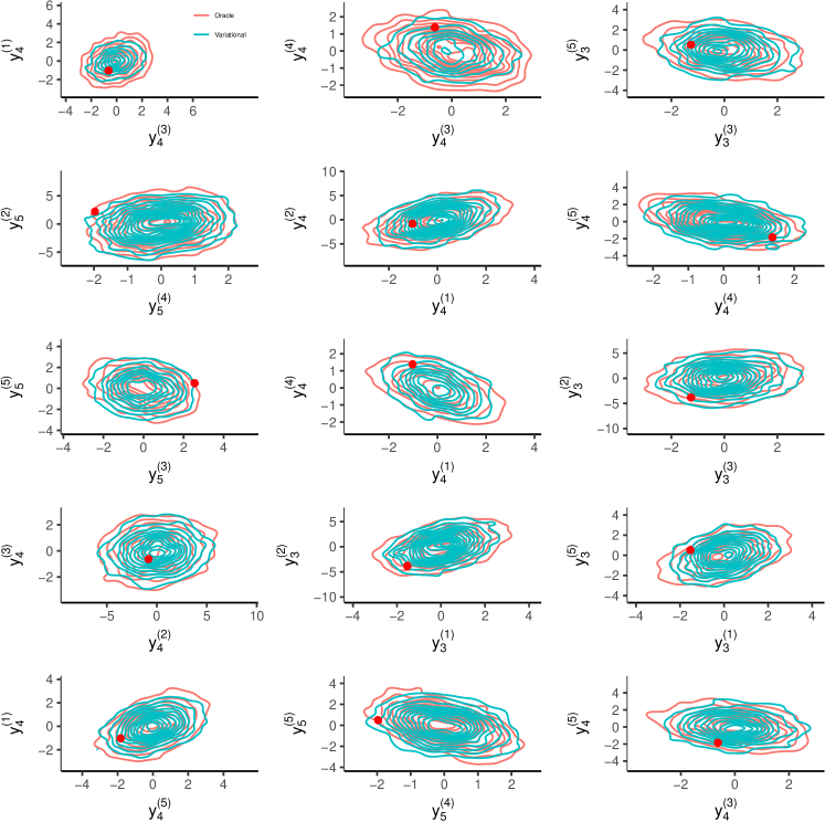
Figure S12: The variational one-step ahead predictive density against the oracle one-step ahead predictive density for simulated data as in Section 6.5. The one-step ahead bivariate predictive densities are shown together with the test observation (red dot). The labels of the axis show which $T+1$ and pair of variables is considered.

S6 Details on the parsimony of the VB parametrization in the applications.

Tables S1 and S2 provides further details of the number of Gaussian variational parameters in the different parts of the variational structure for the spatio-temporal model and the Wishart process example, respectively.

Table S1: Parsimony of different VB parametrizations in the spatio-temporal model. The table shows the number of variational parameters in the different VB parametrizations obtained by combining either low-rank state / low-rank state and auxiliary (LR-S / LR-SA) with either of low-dimensional state mean / high-dimensional state mean (LD-SM / HD-SM). The variational parameters for the different VB parametrizations (with $T=18$) are divided into $\mu,B,D,C_{1}$ and $C_{2}$ defined in Section 4. The saturated Gaussian variational approximation has $8,923,199$ parameters when $\theta$ is 4223 dimensional.

Parametrization		$\mu$		$B$		$D$		$C_{1}$		$C_{2}$		$\mathrm{Total}$
LR-S + LD-SM		$2,190$		$438$		$2,109$		$370$		$4,447$		$9,554$
LR-S + HD-SM		$4,223$		$438$		$2,109$		$370$		$4,447$		$11,587$
LR-SA + LD-SM		$264$		$876$		$4,107$		$730$		$451$		$6,428$
LR-SA + HD-SM		$4,223$		$876$		$4,107$		$730$		$451$		$10,387$

Table S2: Parsimony of different VB parametrizations in the Wishart process example. The table shows the number of variational parameters in the different VB parametrizations obtained by the low-dimensional state mean / high-dimensional state mean (LD-SM / HD-SM). The variational parameters for the different VB parametrizations (with $T=100$) are divided into $\mu,B,D,C_{1}$ and $C_{2}$ defined in Section 4 for two different examples. The first example is model $\mathrm{M}_{1}$ which is benchmarked against MCMC which has $k=5$ ($p=15$). The second example, $\mathrm{M}_{2}$, has $k=12$ ($p=78$), with only the LD-SM parametrization considered. The saturated Gaussian variational approximation for model $\mathrm{M}_{1}$ has $1,152,920$ variational parameters with $\theta$ ${1517}$ dimensional. For $model\mathrm{M}_{2}$, the corresponding number of variational parameters is $31,059,020$ with with $\theta$ ${7880}$ dimensional.

Parametrization		$\mu$		$B$		$D$		$C_{1}$		$C_{2}$		$\mathrm{Total}$
$\mathrm{M}_{1}$ - LD-SM		$417$		$54$		$1,500$		$1,990$		$48$		$4,009$
$\mathrm{M}_{1}$ - HD-SM		$1,517$		$54$		$1,500$		$1,990$		$48$		$5,109$
$\mathrm{M}_{2}$ - LD-SM		$480$		$306$		$7,800$		$1,990$		$237$		$10,813$

S7 The problem with the Philipov and Glickman, 2006b MCMC implementation of their stochastic volatility model

Following from Section 6.1, we now discuss why the MCMC in Philipov and Glickman, 2006b , as corrected by Rinnergschwentner et al., (2012), is infeasible for this problem. Rinnergschwentner et al., (2012) shows that $A^{-1}$ cannot be sampled directly from a Wishart distribution in a Gibbs sampling step. We tried implementing a random-walk Metropolis-Hastings update for $A^{-1}$ using a Wishart proposal with a mean equal to the current value in the MCMC. The erroneous step also results in changes for all the full conditionals, which explains why our implementation does not achieve the sampling efficiency reported in Philipov and Glickman, 2006b when $k=5$. Figure S13 shows that the MCMC iterates are highly correlated, leading to small values for the effective sample size; leads to unreliable highly variable kernel density estimates of posterior densities. and is the reason we benchmark the adequacy of the variational approximation using the oracle predictive density approach in Section 6.5.

Therefore, this application is infeasible for this particular Metropolis-Hastings within Gibbs sampler when $k=5$; it gets even worse for $k=12$, and the main reasons the sampler fails are due to an independent Wishart proposal within Gibbs for updating $\Sigma^{-1}_{t}$ for $t<T$ (at $t=T$ perfect sampling from a Wishart can be applied) and the random-walk proposal within Gibbs for $A^{-1}$. It is well known that these proposals fail in a high-dimensional setting: the random-walk explores the sampling space very slowly while independent samplers get stuck, i.e. reject nearly all attempts to move the Markov chain.

We remark that other MCMC approaches for estimating this model more efficiently might be possible, but it is outside the scope of this paper to pursue this. As an example, Hamiltonian Monte Carlo on the Riemannian manifold (Girolami and Calderhead,, 2011) has proven to be effective in sampling models with $500\text{-}1,000$ parameters. However, the computational burden relative to standard MCMC is increased and, moreover, tuning the algorithm becomes more difficult.

Figure S13: Autocorrelation function (ACF) plots for the MCMC iterates of $A$, $\nu$ and $d$.

References

• Aguilar and West, (2000) Aguilar, O. and West, M. (2000). Bayesian dynamic factor models and portfolio allocation. Journal of Business & Economic Statistics, 18(3):338–357.
• Andrieu et al., (2010) Andrieu, C., Doucet, A., and Holenstein, R. (2010). Particle Markov chain Monte Carlo methods. Journal of the Royal Statistical Society, Series B, 72:1–33.
• Andrieu and Roberts, (2009) Andrieu, C. and Roberts, G. (2009). The pseudo-marginal approach for efficient Monte Carlo computations. The Annals of Statistics, 37:697–725.
• Archer et al., (2016) Archer, E., Park, I. M., Buesing, L., Cunningham, J., and Paninski, L. (2016). Black box variational inference for state space models. arXiv:1511.07367 ANY UPDATE.
• Attias, (1999) Attias, H. (1999). Inferring parameters and structure of latent variable models by variational Bayes. In Laskey, K. and Prade, H., editors, Proceedings of the 15th Conference on Uncertainty in Artificial Intelligence, pages 21–30. Morgan Kaufmann.
• Barber and Bishop, (1998) Barber, D. and Bishop, C. M. (1998). Ensemble learning for multi-layer networks. In Jordan, M. I., Kearns, M. J., and Solla, S. A., editors, Advances in Neural Information Processing Systems 10, pages 395–401. MIT Press.
• Bartholomew et al., (2011) Bartholomew, D. J., Knott, M., and Moustaki, I. (2011). Latent variable models and factor analysis: A unified approach, 3rd edition. John Wiley & Sons.
• Beaumont, (2003) Beaumont, M. A. (2003). Estimation of population growth or decline in genetically monitored populations. Genetics, 164:1139–1160.
• Blei et al., (2017) Blei, D. M., Kucukelbir, A., and McAuliffe, J. D. (2017). Variational inference: A review for statisticians. Journal of the American Statistical Association, 112(518):859–877.
• Bottou, (2010) Bottou, L. (2010). Large-scale machine learning with stochastic gradient descent. In Lechevallier, Y. and Saporta, G., editors, Proceedings of the 19th International Conference on Computational Statistics (COMPSTAT’2010), pages 177–187. Springer.
• Carlin et al., (1992) Carlin, B. P., Polson, N. G., and Stoffer, D. S. (1992). A Monte Carlo approach to nonnormal and nonlinear state-space modeling. Journal of the American Statistical Association, 87(418):493–500.
• Carter and Kohn, (1994) Carter, C. K. and Kohn, R. (1994). On Gibbs sampling for state space models. Biometrika, 81(3):541–553.
• Carvalho et al., (2008) Carvalho, C. M., Chang, J., Lucas, J. E., Nevins, J. R., Wang, Q., and West, M. (2008). High-dimensional sparse factor modeling: Applications in gene expression genomics. Journal of the American Statistical Association, 103(484):1438–1456.
• Caswell and van Daalen, (2016) Caswell, H. and van Daalen, S. F. (2016). A note on the vec operator applied to unbalanced block-structured matrices. Journal of Applied Mathematics. Article ID 4590817.
• Challis and Barber, (2013) Challis, E. and Barber, D. (2013). Gaussian Kullback-Leibler approximate inference. Journal of Machine Learning Research, 14:2239–2286.
• Cressie and Wikle, (2011) Cressie, N. and Wikle, C. (2011). Statistics for Spatio-Temporal Data. Wiley.
• Doucet et al., (2015) Doucet, A., Pitt, M. K., Deligiannidis, G., and Kohn, R. (2015). Efficient implementation of Markov chain Monte Carlo when using an unbiased likelihood estimator. Biometrika, 102:295–313.
• Durrande et al., (2019) Durrande, N., Adam, V., Bordeaux, L., Eleftheriadis, S., and Hensman, J. (2019). Banded matrix operators for gaussian markov models in the automatic differentiation era. In Chaudhuri, K. and Sugiyama, M., editors, Proceedings of Machine Learning Research, volume 89 of Proceedings of Machine Learning Research, pages 2780–2789. PMLR.
• Gelman and Rubin, (1992) Gelman, A. and Rubin, D. B. (1992). Inference from iterative simulation using multiple sequences. Statistical Science, pages 457–472.
• Geweke and Zhou, (1996) Geweke, J. and Zhou, G. (1996). Measuring the pricing error of the arbitrage pricing theory. Review of Financial Studies, 9(2):557–587.
• Girolami and Calderhead, (2011) Girolami, M. and Calderhead, B. (2011). Riemann manifold Langevin and Hamiltonian Monte Carlo methods. Journal of the Royal Statistical Society: Series B (Statistical Methodology), 73(2):123–214.
• Gordon et al., (1993) Gordon, N. J., Salmond, D. J., and Smith, A. F. (1993). Novel approach to nonlinear/non-Gaussian Bayesian state estimation. In IEE Proceedings F (Radar and Signal Processing), volume 140, pages 107–113. IET.
• Han et al., (2016) Han, S., Liao, X., Dunson, D. B., and Carin, L. C. (2016). Variational Gaussian copula inference. In Gretton, A. and Robert, C. C., editors, Proceedings of the 19th International Conference on Artificial Intelligence and Statistics, volume 51, pages 829–838, Cadiz, Spain. JMLR Workshop and Conference Proceedings.
• Hoffman et al., (2013) Hoffman, M. D., Blei, D. M., Wang, C., and Paisley, J. (2013). Stochastic variational inference. Journal of Machine Learning Research, 14:1303–1347.
• Ji et al., (2010) Ji, C., Shen, H., and West, M. (2010). Bounded approximations for marginal likelihoods. Technical Report 10-05, Institute of Decision Sciences, Duke University. ANY UPDATE ??
• Jordan et al., (1999) Jordan, M. I., Ghahramani, Z., Jaakkola, T. S., and Saul, L. K. (1999). An introduction to variational methods for graphical models. Machine Learning, 37:183–233.
• Kingma and Welling, (2014) Kingma, D. P. and Welling, M. (2014). Auto-encoding variational Bayes. In Proceedings of the 2nd International Conference on Learning Representations (ICLR) 2014. https://arxiv.org/abs/1312.6114.
• Ku et al., (2014) Ku, Y.-C., Bloomfield, P., and Ghosh, S. K. (2014). A flexible observed factor model with separate dynamics for the factor volatilities and their correlation matrix. Statistical Modelling, 14(1):1–20.
• Kucukelbir et al., (2017) Kucukelbir, A., Tran, D., Ranganath, R., Gelman, A., and Blei, D. M. (2017). Automatic differentiation variational inference. Journal of Machine Learning Research, 18(14):1–45.
• Lopes et al., (2008) Lopes, H. F., Salazar, E., and Gamerman, D. (2008). Spatial dynamic factor analysis. Bayesian Analysis, 3(4):759–792.
• Magnus, (1985) Magnus, J. R. (1985). On differentiating eigenvalues and eigenvectors. Econometric Theory, 1:179–191.
• Magnus and Neudecker, (1980) Magnus, J. R. and Neudecker, H. (1980). The elimination matrix: some lemmas and applications. SIAM Journal on Algebraic Discrete Methods, 1(4):422–449.
• Magnus and Neudecker, (1985) Magnus, J. R. and Neudecker, H. (1985). Matrix differential calculus with applications to simple, Hadamard, and Kronecker products. Journal of Mathematical Psychology, 29:474–492.
• Miller et al., (2017) Miller, A. C., Foti, N. J., and Adams, R. P. (2017). Variational boosting: Iteratively refining posterior approximations. In Proceedings of the 34th International Conference on Machine Learning-Volume 70, pages 2420–2429. JMLR. org.
• Nott et al., (2012) Nott, D. J., Tan, S. L., Villani, M., and Kohn, R. (2012). Regression density estimation with variational methods and stochastic approximation. Journal of Computational and Graphical Statistics, 21:797–820.
• Ong et al., (2018) Ong, V. M.-H., Nott, D. J., and Smith, M. S. (2018). Gaussian variational approximation with a factor covariance structure. Journal of Computational and Graphical Statistics, 27(3):465–478.
• Opper and Archambeau, (2009) Opper, M. and Archambeau, C. (2009). The variational Gaussian approximation revisited. Neural Computation, 21:786–792.
• Ormerod and Wand, (2010) Ormerod, J. T. and Wand, M. P. (2010). Explaining variational approximations. The American Statistician, 64:140–153.
• Paisley et al., (2012) Paisley, J. W., Blei, D. M., and Jordan, M. I. (2012). Variational Bayesian inference with stochastic search. In Langford, J. and Pineau, J., editors, Proceedings of the 29th International Conference on Machine Learning, ICML 2012. http://icml.cc/2012/papers/687.pdf.
• (40) Philipov, A. and Glickman, M. E. (2006a). Factor multivariate stochastic volatility via Wishart processes. Econometric Reviews, 25(2-3):311–334.
• (41) Philipov, A. and Glickman, M. E. (2006b). Multivariate stochastic volatility via Wishart processes. Journal of Business & Economic Statistics, 24(3):313–328.
• Pitt et al., (2012) Pitt, M. K., dos Santos Silva, R., Giordani, P., and Kohn, R. (2012). On some properties of Markov chain Monte Carlo simulation methods based on the particle filter. Journal of Econometrics, 171(2):134–151.
• Plummer et al., (2006) Plummer, M., Best, N., Cowles, K., and Vines, K. (2006). CODA: convergence diagnosis and output analysis for MCMC. R News, 6(1):7–11.
• Ranganath et al., (2014) Ranganath, R., Gerrish, S., and Blei, D. M. (2014). Black box variational inference. In Kaski, S. and Corander, J., editors, Proceedings of the 17th International Conference on Artificial Intelligence and Statistics, volume 33, pages 814–822. JMLR Workshop and Conference Proceedings.
• Rezende et al., (2014) Rezende, D. J., Mohamed, S., and Wierstra, D. (2014). Stochastic backpropagation and approximate inference in deep generative models. In Xing, E. P. and Jebara, T., editors, Proceedings of the 29th International Conference on Machine Learning, ICML 2014. proceedings.mlr.press/v32/rezende14.pdf.
• Rinnergschwentner et al., (2012) Rinnergschwentner, W., Tappeiner, G., and Walde, J. (2012). Multivariate stochastic volatility via Wishart processes: A comment. Journal of Business & Economic Statistics, 30(1):164–164.
• Robbins and Monro, (1951) Robbins, H. and Monro, S. (1951). A stochastic approximation method. The Annals of Mathematical Statistics, 22:400–407.
• Roeder et al., (2017) Roeder, G., Wu, Y., and Duvenaud, D. (2017). Sticking the landing: Simple, lower-variance gradient estimators for variational inference. arXiv preprint arXiv:1703.09194.
• Salimans and Knowles, (2013) Salimans, T. and Knowles, D. A. (2013). Fixed-form variational posterior approximation through stochastic linear regression. Bayesian Analysis, 8:837–882.
• Seeger, (2000) Seeger, M. (2000). Bayesian model selection for support vector machines, Gaussian processes and other kernel classifiers. In Solla, S. A., Leen, T. K., and Müller, K., editors, Advances in Neural Information Processing Systems 12, pages 603–609. MIT Press.
• Shapiro, (1985) Shapiro, A. (1985). Identifiability of factor analysis: Some results and open problems. Linear Algebra and its Applications, 70:1–7.
• Smith et al., (2019) Smith, M. S., Loaiza-Maya, R., and Nott, D. J. (2019). High-dimensional copula variational approximation through transformation. arXiv preprint arXiv:1904.07495.
• Spantini et al., (2018) Spantini, A., Bigoni, D., and Marzouk, Y. (2018). Inference via low-dimensional couplings. Journal of Machine Learning Research, 19(66):1–71.
• Tan et al., (2019) Tan, L. S.-L., Bhaskaran, A., and Nott, D. J. (2019). Conditionally structured variational Gaussian approximation with importance weights. arXiv preprint arXiv:1904.09591.
• Tan and Nott, (2017) Tan, S. L. and Nott, D. J. (2017). Gaussian variational approximation with sparse precision matrices. Statistics and Computing, PUT in volume:1–17.