The RINGS Survey III: Medium-Resolution H$\alpha$ Fabry-Pérot Kinematic Dataset

Abstract

The distributions of stars, gas, and dark matter in disk galaxies provide important constraints on galaxy formation models, particularly on small spatial scales ($<$1 kpc). We have designed the RSS Imaging spectroscopy Nearby Galaxy Survey (RINGS) to target a sample of 19 nearby spiral galaxies. For each of these galaxies, we are obtaining and modeling H$\alpha$ and H I 21 cm spectroscopic data as well as multi-band photometric data. We intend to use these models to explore the underlying structure and evolution of these galaxies in a cosmological context, as well as whether the predictions of $\rm{\Lambda}$CDM are consistent with the mass distributions of these galaxies. In this paper, we present spectroscopic imaging data for 14 of the RINGS galaxies observed with the medium spectral resolution Fabry-Pérot etalon on the Southern African Large Telescope. From these observations, we derive high spatial resolution line of sight velocity fields of the H$\alpha$ line of excited hydrogen, as well as maps and azimuthally averaged profiles of the integrated H$\alpha$ and [N II] emission and oxygen abundances. We then model these kinematic maps with axisymmetric models, from which we extract rotation curves and projection geometries for these galaxies. We show that our derived rotation curves agree well with other determinations and the similarity of the projection angles with those derived from our photometric images argues against these galaxies having intrinsically oval disks.

1. Introduction

The standard cosmological paradigm of Cold Dark Matter with the addition of a cosmological constant ($\rm{\Lambda}$CDM) has been successful at interpreting astrophysical phenomena on a wide range of scales, from the large scale structure of the Universe to the formation of individual galaxies (Somerville & Davé, 2015). However, it remains somewhat unclear whether the internal structures of simulated galaxies formed in a $\rm{\Lambda}$CDM framework are consistent with observations of real galaxies.

In spiral galaxies, the structure of dark matter halos can be constrained using galaxy rotation curves (e.g. Bosma, 1978). Typically, the observed rotation curve is decomposed into contributions from stars and gas and any remaining velocity is attributed to dark matter. In cosmological simulations of dark matter structure growth, dark matter halos have been observed to follow a broken power law form (e.g. Einasto, 1965; Navarro et al., 1996, 2004; Gao et al., 2008). To account for the additional gravitational pull provided by baryons, modifications can be applied to theoretical halo density profiles to increase their densities at small radii (e.g. Gnedin et al., 2004; Sellwood & McGaugh, 2005). Applying these modified halo models to observed rotation curves produces dark matter halos which are underdense relative to the predictions of $\rm{\Lambda}$CDM simulations (Papastergis et al., 2015).

Numerical simulations which incorporate stellar feedback in galaxies have partially eased this tension by showing that feedback from baryonic processes can redistribute dark matter within a galaxy (Governato et al., 2010; Pontzen & Governato, 2012; Teyssier et al., 2013). These effects are stronger in galaxies with lower masses (e.g. Oh et al., 2011; Brook et al., 2011; Pontzen & Governato, 2014). Recent simulations have shown that the ability of a galaxy to redistribute dark matter through stellar feedback depends on the ratio of its stellar mass to its halo mass (e.g. Di Cintio et al., 2014; Brook, 2015). These $M_{*}/M_{\rm halo}$-dependent density profiles have been shown by Katz et al. (2017) to be more consistent with the photometry and rotation curves of real galaxies than traditional NFW profiles.

The relationship between dark matter halos and observed rotation curves is not a trivial one, as measurements of rotation curves can be biased by non-circular motions, projection effects, and halo triaxiality (e.g. Rhee et al., 2004; Hayashi & Navarro, 2006; Valenzuela et al., 2007). Measurements of one-dimensional rotation curves are therefore insufficient to constrain the three-dimensional mass distributions. All of these mechanisms for potential bias in rotation curves leave kinematic signatures in the full three-dimensional velocity distributions of galaxy disks. For example, gas streaming along bars and spiral arms has both circular and radial components to its velocity, and therefore will affect the line of sight velocities along the major and minor axes differently (Sellwood & Zánmar Sánchez, 2010).

Measurements of the velocity field of the entire disk at high spatial resolution are required to extract these kinematic signatures. For example, to separate bar-like flows in spiral galaxies from their rotation curves, $<200~{}$pc spatial resolution is required (e.g. Marinova & Jogee, 2007; Sellwood & Zánmar Sánchez, 2010; Barrera-Ballesteros et al., 2014; Holmes et al., 2015).

In recent years, the state of the art in numerical simulations has moved to smaller and smaller spatial scales. However, comparisons of these simulations to observed galaxies have been lacking, partially due to a lack of velocity fields of sufficiently high resolution for comparison.

We have designed the RSS Imaging spectroscopy Nearby Galaxy Survey (RINGS) to obtain the high-resolution kinematic data necessary to probe these open questions of galaxy structure. Our survey targets 19 nearby, late-type spiral galaxies over a wide range of masses (67 km s${}^{-1}<V_{\rm flat}<$ 275 km s^-1) and luminosities (-17.5 $>M_{V}>$ -21.5). The survey is designed to exploit the large collecting area and large field-of-view of the Robert Stobie Spectrograph (RSS) on the Southern African Large Telescope (SALT). In addition to the high spatial resolution H$\alpha$ kinematic data from SALT’s RSS, we are obtaining lower spatial resolution H I 21 cm kinematic observations and have obtained $BVRI$ photometric imaging of these galaxies.

A number of previous surveys have obtained two-dimensional H$\alpha$ velocity fields of galaxies with similar goals to RINGS, e.g. BH$\alpha$BAR (Hernandez et al., 2005), GHASP (Epinat et al., 2008), GH$\alpha$FaS (Hernandez et al., 2008), DiskMass (Bershady et al., 2010), and CALIFA (Sánchez et al., 2012). Compared to these surveys, our data are deeper and more extended thanks to SALT’s large primary mirror and large angular field-of-view. The typical angular resolution of the RINGS data is similar to that of the DiskMass and CALIFA surveys and somewhat worse than that of GH$\alpha$FaS. However, the RINGS galaxies are typically more nearby than the galaxies in those surveys, and our physical resolutions are comparable to those of GH$\alpha$FaS and higher than those of DiskMass and CALIFA. The typical spectral resolution of our data ($R\sim 1300$) is similar to that of CALIFA ($R\sim 1000$) and lower than that of DiskMass ($R\sim 8000$) and GH$\alpha$FaS ($R\sim 15000$). Our target selection criteria also differ from these surveys in choosing a representative sample of partially inclined galaxies across a wide range of Hubble classifications, masses, and luminosities.

In Paper I (Mitchell et al., 2015), we presented our first H$\alpha$ and H I kinematic data and modelling for the galaxy NGC 2280. In Paper II (Kuzio de Naray et al., in prep.), we presented our photometric sample and modelling. In this paper, we present kinematic maps and axisymmetric models of 14 of the 19 RINGS galaxies. The maps are derived from data taken using the medium-resolution etalon of SALT’s Fabry-Pérot system. The typical angular resolution of our resulting H$\alpha$ velocity fields is $\sim 2.5\arcsec$, corresponding to a typical spatial resolution of $\sim 250~{}$pc at the source locations. We then model the kinematic data using the DiskFit software package (Spekkens & Sellwood, 2007; Sellwood & Zánmar Sánchez, 2010) and show that the derived rotation curves generally agree well with others in the literature. We also compare the fitted projection parameters with those obtained from our I-band images. Finally, we present azimuthally-averaged H$\alpha$ and [N II] profiles for these galaxies, which we use to derive oxygen abundance gradients. In future papers in this series, we will use our velocity maps in order to better understand these galaxies’ mass distributions.

Table 1RINGS Medium-Resolution Fabry-PérotObservations

Galaxy	Class	Obs. Date	Exp. Time	Seeing	$\sigma_{\lambda}$ [Å]	Npix	Nelem	$D$ [Mpc]	Scale [pc/″]	Seeing	$M_{I}$
NGC 337A	SAB(s)dm	11 Sept 2012	22$\times$100s	1.7″	0.054	9448	1842	2.57	12.5	30 pc	-16.7
		10 Oct 2012	26$\times$91s	2.1″	0.028
		12 Oct 2012	26$\times$38s	2.4″	0.064
NGC 578	SAB(rs)c	29 Dec 2011	28$\times$50s	1.8″	0.025	29890	4416	27.1	131	370 pc	-22.5
		23 Oct 2012	23$\times$98s	2.8″	0.036
NGC 908	SA(s)c	1 Nov 2011	41$\times$60s	2.2″	0.033	28045	4284	19.4	94.1	220 pc	-21.6
		28 Dec 2011	25$\times$100s	2.3″	0.034
NGC 1325	SA(s)bc	1 Nov 2011	24$\times$90s	2.0″	0.025	7813	1532	23.7	115	310 pc	-21.3
		28 Dec 2011	23$\times$100s	2.7″	0.026
NGC 1964	SAB(s)b	2 Apr 2012	23$\times$70s	2.4″	0.025	12093	2220	20.9	101	270 pc	-21.8
		1 Feb 2013	25$\times$80s	2.7″	0.031
NGC 2280	SA(s)cd	1 Nov 2011	25$\times$60s	2.0″	0.040	27198	6609	24.0	116	260 pc	-20.8
		28 Dec 2011	26$\times$50s	2.2″	0.049
NGC 3705	SAB(r)ab	1 Feb 2013	23$\times$77s	2.3″	0.10	6687	1394	18.5	89.7	230 pc	-19.9
		26 Feb 2014	23$\times$80s	2.6″	0.064
NGC 4517A	SB(rs)dm	23 Apr 2012	37$\times$80s	2.5″	0.049	2904	592	26.7	129	360 pc	-22.8
		27 Apr 2015	20$\times$90s	2.8″	0.070
		27 Apr 2015	21$\times$102s	2.3″	0.19
		7 May 2015	21$\times$95s	2.3″	0.21
		7 May 2015	21$\times$100s	1.9″	0.21
NGC 4939	SA(s)bc	14 Apr 2013	24$\times$90s	1.9″	0.051	18971	4809	41.6	202	420 pc	-22.9
		27 Apr 2015	24$\times$95s	2.1″	0.062
NGC 5364	SA(rs)bc pec	28 May 2012	24$\times$80s	2.0″	0.087	14756	4720	18.1	87.8	180 pc	-21.2
NGC 6118	SA(s)cd	28 May 2012	22$\times$100s	2.0″	0.052	14207	3686	22.9	111	220 pc	-22.7
		2 Sept 2012	22$\times$85s	1.8″	0.038
NGC 6384	SAB(r)bc	15 July 2014	23$\times$85s	2.5″	0.062	17442	3760	19.7	95.5	260 pc	-21.8
		31 July 2014	23$\times$85s	2.7″	0.077
NGC 7606	SA(s)b	17 Aug 2014	13$\times$87s	2.2″	0.073	10454	1835	34.0	165	460 pc	-24.4
		1 Sept 2014	26$\times$85s	1.7″	0.11
		6 Aug 2015	22$\times$92s	2.8″	0.15
NGC 7793	SA(s)d	2 Sept 2014	22$\times$90s	2.1″	0.027	101908	12028	3.44	16.7	50 pc	-18.5
		3 Sept 2014	18$\times$90s	2.7″	0.072
		8 June 2015	22$\times$90s	2.6″	0.10
		14 Aug 2015	18$\times$90s	3.0″	0.13
		21 Aug 2015	20$\times$80s	3.0″	0.084

Note. — A summary of our observations and resulting kinematic maps for the 14 galaxies presented here. From left to right, columns are: (1) galaxy name, (2) morphological classification, (3) observation date, (4) number of exposures and time per exposure, (5) effective seeing with worst seeing for each galaxy marked in bold, (6) estimated uncertainty in our wavelength solution, (7) number of pixels in our fitted maps, (8) number of independent resolution elements in our fitted maps, (9) redshift-independent distance and reference, (10) angular scale at the distances in column 9, (11) seeing in physical units at the distances in column 9, and (12) absolute I-band magnitude derived from the photometry of Kuzio de Naray et al. (in prep.) and the distances in column 9.

2. Data Acquisition and Reduction

We obtained data on 14 nearby late-type galaxies with the medium-resolution mode of the Fabry-Pérot interferometer on the RSS of SALT. Our data were acquired over a total exposure time of 19 hours during the period 11 Nov 2011 to 8 Sept 2015. A typical single observation consists of $\sim 25$ exposures, each of length $\sim 70~{}$seconds. The medium-resolution etalon has a spectral full width at half maximum (FWHM) at H$\alpha$ of $\sim 5~{}$Å. For each exposure taken in an observation, we offset the wavelength of the etalon’s peak transmission by $\sim 2~{}$Å from the previous exposure. Each observation therefore represents a scan over a $\sim 50~{}$Å range in $\sim 2~{}$Å steps. For each galaxy, we attempted to obtain at least two such observations. A summary of the properties of these 14 galaxies and our observations is provided in Table 1.

Note that NGC 2280, which we have discussed previously in Mitchell et al. (2015), is among the galaxies presented in this work. Because several aspects of our data reduction process have changed somewhat (e.g. flat-field correction and ghost subtraction, discussed below) since that work was published, we have chosen to present an updated velocity field of that galaxy here to ensure homogeneity across the final sample.

2.1. Preliminary Data Reduction

We have utilized the PySALT (Crawford et al., 2010) software package to perform preliminary reductions of our raw SALT images. The tasks in PySALT apply standard routines for gain variation corrections, bias subtraction, CCD crosstalk corrections, and cosmic ray removal.

2.2. Flattening

The unusual design of SALT introduces unique challenges in calibrating the intensity of our images. SALT’s primary mirror is composed of a hexagonal grid of 91 1-meter mirrors. Unlike most telescopes, the primary mirror remains stationary over the course of an observation and object tracking is accomplished by moving the secondary optics package in the primary mirror’s focal plane. The full collecting area of the primary mirror is rarely utilized, as some mirror segments are unable to illuminate the secondary depending on a target’s position. Overall, the available collecting area of the primary mirror is smaller by $\sim 30$% at the beginning and end of an observation relative to the middle.

The individual mirror segments are removed for realuminization and replaced on $\sim$weekly timescales in a sequential scheme. This results in the reflectivity of the primary mirror varying as a function of position on the mirror, and these variations change over time as different mirror segments are freshly realuminized.

As a target galaxy passes through SALT’s field of view, individual mirror segments pass in and out of the secondary payload’s field of view, changing the fraction of the total collecting area utilized as a function of time.

Furthermore, differential vignetting of images occurs within the spherical aberration corrector (SAC) on the secondary payload. This effect also varies as a function of object position overhead (as the secondary package moves through the focal plane to track an object). This vignetting effect changes image intensities by $\sim 5-10$% across an image.

The combined effects of these factors result in image intensity variations which are: position-dependent within a single image, pointing-dependent over the course of an observation as the target drifts overhead, and time-dependent over the $\sim$weekly segment-replacement timescale.

A traditional approach to flat-field calibration (i.e. combining several exposures of the twilight sky) is insufficient for correcting these effects, as this approach will not account for the pointing-dependent effects. Theoretical modelling of the sensitivity variations by ray-tracing software is not feasible due to the frequent replacement of mirror segments with different reflective properties.

In a previous paper (Mitchell et al., 2015), we utilized an approach for NGC 2280 which compared stellar photometry in our SALT Fabry-Pérot images to R-band images from the CTIO 0.9m telescope (Kuzio de Naray et al., in prep.). For $\sim 50$ stars present in both sets of images, we computed an intensity ratio between our SALT images and the R-band image. For each SALT image, we then fitted a quadratic two-dimensional polynomial to these intensity ratios. By scaling each of our images by its corresponding polynomial, we were able to correct for these variations.

Unlike NGC 2280, most of our target galaxies do not overlap with dense star fields and we therefore cannot apply this approach. Instead, we have developed a new approach which utilizes the night sky background to calibrate our photometry. We make the assumption that the intrinsic night sky background has uniform intensity over the $8\arcmin$ field of view over the course of each individual exposure ($\sim 70~{}$s). We then mask objects in our fields using a sigma-clipped cutoff for stars and a large elliptical mask for the galaxy. We fit the remaining pixels with a quadratic two-dimensional polynomial of the same form used in the stellar photometry approach described above. We then scale the pixel values in each image by this fitted polynomial. If the assumption of uniform sky brightness is valid, this method results in a uniformly illuminated field.

In order to validate the assumption of uniform sky intensity, we have applied this “sky-fitting” approach to our data on NGC 2280 and compared it to our previous “star-fitting” approach for the same data. We found no significant differences in the resulting fitted polynomials for either of the two nights for which we had data on that galaxy. This suggests that the sky-fitting approach is sufficient for flattening our images. The assumption of a uniform sky background is less likely to be valid if a target galaxy fills a large fraction of the field of view, as is the case with our observations of NGC 7793. We have examined several spectra obtained from overlapping observations of this galaxy, and it appears any errors introduced by a non-uniform sky background are small compared to other sources of uncertainty.

We utilize this “sky-fitting” approach to flat-field correction for all 14 of the galaxies presented in this work.

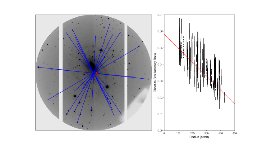
Figure 1.— Left: A median-combined image of our 15 July 2014 observations of NGC 6384 with detected star-ghost pairs marked with blue lines. The large red star marks the location of the point about which the intensity ratios of a ghost to its star are symmetric. The large rectangular feature in the lower-right portion of the left panel is the shadow of SALT’s tracking probe and the affected pixels have been masked from any calculations. Right: The black points with error bars mark the intensity ratios between ghosts and stars as a function of radius from the point marked in the left panel. These star/ghost pairs were selected from all of our SALT Fabry-Pérot observations. The solid red line shows our linear fit to these intensity ratios.

2.3. Ghost identification and subtraction

Reflections between the Fabry-Pérot etalon and the CCD detector result in each light source in an image appearing twice – once at its true position and again at a reflected position, known as the “diametric ghost” (Jones et al., 2002). The positions of these reflections are symmetric about a single point in the image, the location at which the instrument’s optical axis intersects the plane of the CCD. The left panel of Figure 1 illustrates this effect in one of our observations of NGC 6384.

As will be discussed in §2.5, the wavelength calibration solutions for our images are symmetric about the same central point. The ghost positions are therefore extremely useful for precisely determining the location of this point. By matching each star in an image to its ghost and averaging their positions, we are able to determine our reflection centers to within a small fraction of a pixel.

While useful for determining the location of the symmetry axis, the presence of these ghosts adversely affects our goal of measuring velocities. In particular, the reflected image of a target galaxy often overlaps with the galaxy itself. This effect is extremely undesirable, since it mixes emission from gas at one location and velocity with emission from gas at a different location and velocity.

In order to remove them, we perform aperture photometry on each star-ghost pair to determine intensity ratios between the ghosts and their real counterparts. These ratios are typically $\sim 5$%. In a previous paper (Mitchell et al., 2015), we simply rotated each image by 180° about its symmetry axis and subtracted a small multiple of the rotated image from the original. After examining a much larger quantity of data, it appears that the intensity ratio between an object and its ghost depends linearly on the object’s distance from a central point. This decreasing ghost intensity ratio is caused by vignetting within the camera optics of the non-telecentric reflection from the CCD. This central point’s location is not coincident with the center of reflection (private communication: D. O’Donoghue), but appears to be consistent among all of our observations. The right panel of Figure 1 shows the dependence of the ghost intensity ratio on radius from this point. We have fitted a linear function to the flux ratios of star-ghost pairs in several of our observations, which decreases from $\sim 6$% at the central point to $\sim 2$% at the edge of the images. We then apply the same reflect-and-subtract approach as in (Mitchell et al., 2015), except that here we rescale the reflected images by this linear function rather than a constant factor. This process removes most of the ghost image intensity from our science images without necessitating masking of these regions.

2.4. Alignment and Normalization

Among the images of a single observation, we use the centroid locations of several stars to align our images to one another. Typically, the image coordinate system drifts by $\sim 0.25$″ over the course of an observation.

As mentioned previously, different fractions of SALT’s primary mirror are utilized over the course of a single observation. Thus, the photometric sensitivity of each image varies over an observational sequence. To correct for this effect, we perform aperture photometry on the same stars which were used for aligning the images in order to determine a normalization factor for each image. We then scale each image by a multiplicative normalization factor so that each of these stars has the same intensity in all of our images. Typically, between 10 and 50 stars are used in this process, though in some extreme cases (e.g. NGC 578), the number of stars in the images can be as low as 5.

The combined effects of flattening uncertainty (§2.2), ghost subtraction (§2.3), and normalization uncertainty (§2.4) result in a typical photometric uncertainty of $\sim 10-12\%$.

When combining multiple observations which were taken at different telescope pointings, we have utilized the astrometry.net software package (Lang et al., 2010) to register our images’ pixel positions to accurate sky coordinates. We then use the resulting astrometric solutions to align our observations to one another.

Just as we used stellar photometry to normalize images from among a single observation sequence, we use the same photometry to normalize different observation sequences to one another. Stars which are visible in only one pointing are not useful for this task, so we use the photometry of stars which are visible in more than one observation sequence.

2.5. Wavelength Calibration

Collimated light incident on the Fabry-Pérot etalon arrives at different angles depending on position in our images. Different angles of incidence result in different wavelengths of constructive interference. Thus, the peak wavelength of an image varies across the image itself. The wavelength of peak transmission is given by

$$\lambda_{\rm peak}(R)=\frac{\lambda_{\rm cen}}{(1+R^{2}/F^{2})^{1/2}}$$ (1)

where $\lambda_{\rm cen}$ is the peak wavelength at the center of the image, $R$ is the radius of a pixel from the image center, and $F$ is the effective focal length of the camera optics, measured in units of pixels. The image center is the location where the optical axis intersects the image plane, and is notably the same as the center of the star-ghost reflections discussed in §2.3.

The peak wavelength at the center is determined by a parameter, $z$, which controls the spacing of the etalon’s parallel plates. It may also be a function of time, as a slight temporal drift in the etalon spacing has been observed. In general, we find that the function

$$\lambda_{\rm cen}(z,t)=A+Bz+Et$$ (2)

is sufficient to describe the central wavelength’s dependence on the control parameter and time. This equation equivalent to the one found by Rangwala et al. (2008) with the addition of a term which is linear in time to account for a slight temporal drift. We find that their higher-order terms proportional to $z^{2}$ and $z^{3}$ are not necessary over our relatively narrow wavelength range.

Across a single image, the wavelength of peak transmission depends only on the radius, $R$. Therefore, a monochromatic source which uniformly illuminates the field will be imaged as a symmetric ring around the image center, with radius $R_{\rm ring}=F(\lambda_{\rm cen}^{2}/\lambda_{\rm ring}^{2}-1)^{1/2}$.

Before and after each observation sequence, exposures of neon lamps were taken for the purposes of wavelength calibrations, which create bright rings in the images. Additionally, several atmospheric emission lines of hydrogen, [N II], and OH are imaged as dim rings in our observations of the RINGS galaxies. By measuring the radii of these rings, we can determine best-fitting values for the constants $A$, $B$, $E$, and $F$ in the above equations using a least-squares minimization fit. We then use these fitted parameters to calibrate the wavelengths in our images. The sixth column of Table 1 shows the uncertainty in each observation’s wavelength solution, calculated as the root mean square residual to our wavelength solution divided by the square root of the number of degrees of freedom in the fit.

2.6. Sky Subtraction

The sky background radiation in our images is composed of two components: a continuum, which we treat as constant with wavelength, and emission lines from molecules in the atmosphere.

Once a wavelength solution has been found for our images, we search in our images for ring signatures of known atmospheric emission lines (Osterbrock et al., 1996). We fit for such emission lines and subtract the fitted profiles from our images. Occasionally, additional emission lines are seen (as prominent rings) even after such subtraction. These emission lines fall into two broad categories: adjacent spectral orders and diffuse interstellar bands.

The medium-resolution Fabry-Pérot system has a free spectral range (FSR) at H$\alpha$ of $\sim 75~{}$Å. Thus, an atmospheric emission line $\pm 75~{}$Å from an image’s true wavelength may appear in the image due to the non-zero transmission of the order-blocking filter at $\pm 75~{}$Å. Several such emission lines have been detected in our data and subsequently fitted and subtracted from our images.

In several of our observations, we have detected emission consistent with the diffuse interstellar band (DIB) wavelength at 6613 Å (Williams et al., 2015). DIBs are commonly seen as absorption lines in stellar spectra, and are not often observed in emission (Herbig, 1995). This emission has also been fitted and subtracted from our data in the same fashion as the known night-sky emission lines. The DIB emission was detected in our observations of NGC 908, NGC 1325, and NGC 2280.

Once ring features from emission lines have been fitted and subtracted, we have run a sigma-clipped statistics algorithm to determine the typical value of the night sky continuum emission. This continuum value is then subtracted from each of our images before we produce our final data cube.

2.7. Convolution to Uniform Seeing

Because atmospheric turbulence and mirror alignment do not remain constant over the course of an observation, each of our images has a slightly different value for the effective seeing FWHM. In producing a data cube, we artificially smear all of our images to the seeing of the worst image of the observation track. In principle, we could choose to keep only images with better effective seeing and discard images with worse seeing. When our observations were obtained, SALT did not have closed-loop control of the alignment of the primary mirror segments. Thus the image quality tended to degrade over an observational sequence. Discarding poorer images would therefore tend to preferentially eliminate the longer wavelength images, since we usually stepped upward in wavelength over the sequence. Discarding images would also reduce the overall depth of our observations. For these reasons, we choose to not discard any images when producing the final data cubes presented in this work.

The correction to uniform seeing is done by convolution with a Gaussian beam kernel with $\sigma_{\rm beam}^{2}=\sigma_{\rm worst}^{2}-\sigma_{\rm image}^{2}$. We also shift the position of the convolution kernel’s center by the values of the shifts calculated from stellar centroids described in §2.4. In this way, we shift and convolve our images simultaneously. The “Seeing” column of Table 1 lists the worst seeing FWHM from each of our observations. Typical worst seeing values are between 2″ and 3″. In the cases where we combine multiple observations of the same object, we convolve all observations to the seeing of the worst image from among all observations of that object, then combine the results into a single data cube.

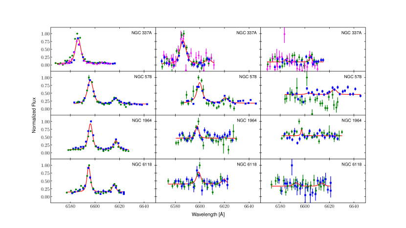
Figure 2.— Selected spectra (solid points with error bars) and best-fitting line profiles (solid red lines) from our data cubes. The left panels show pixels with very high signal-to-noise. The middle panels show pixels with much lower signal-to-noise. The right panels show pixels very low signal-to-noise which are just above our detection thresholds. All spectra have been normalized so that the maximum value of each spectrum is 1. Each row’s spectra are different pixels selected from a single galaxy’s data cube. The different colors and shapes of points correspond to observations from different nights.

2.8. Line Profile Fitting

In addition to observing the H$\alpha$ line, our wavelength range is wide enough to detect the [N II] 6583 line as well. We fit for both of these lines in our spectra simultaneously. The transmission profile of the Fabry-Pérot etalon is well-described by a Voigt function,

$$V(\lambda;\sigma_{g},\gamma_{l})=\int_{-\infty}^{\infty}G(\lambda^{\prime},\sigma_{g})\Gamma(\lambda-\lambda^{\prime},\gamma_{l})d\lambda^{\prime},$$ (3)

where $G(\lambda,\sigma_{g})$ and $\Gamma(\lambda,\gamma_{l})$ are Gaussian and Lorentzian functions, respectively. Calculating this convolution of functions is computationally expensive, and we therefore make use of the pseudo-Voigt function described by Humlíček (1982). At each spatial pixel in our data cubes, we fit a 6-parameter model of the form

$$I(\lambda;C,F_{H},F_{N},\lambda_{H},\sigma_{g},\gamma_{l})=\phantom{junkjunk}$$

$$\phantom{junkjunk}C+F_{H}V(\lambda-\lambda_{H};\sigma_{g},\gamma_{l})+$$

$$\phantom{junkjunk}F_{N}V(\lambda-1.003137\lambda_{H};\sigma_{g},\gamma_{l}),$$ (4)

where $I(\lambda;\ldots)$ is the image intensity as a function of wavelength and the 6 model parameters are: $C$, the continuum surface brightness, $F_{H}$, the integrated surface brightness of the H$\alpha$ line, $F_{N}$, the integrated surface brightness of the [N II] 6583 line, $\lambda_{H}$, the peak wavelength of Doppler-shifted H$\alpha$, and $\sigma_{g}$ and $\gamma_{l}$ the two line widths of the Voigt profile. We assume that the H$\alpha$ and [N II] 6583 emission arise from gas at the same velocity, and the factor of 1.003137 in the above equation reflects this assumption.

An anonymous referee questioned whether $C$ would really be constant over the fitted range because the stellar continuum would have an H$\alpha$ absorption feature at almost the same wavelength as the H$\alpha$ emission we are attempting to measure. While there may be some effect of stellar H$\alpha$ absorption on the emission line strength, it is unlikely to exactly cancel the gaseous emission, and would leave a distorted spectral profile (e.g. with emission core and absorption wings), which we do not see. Rosa-González et al. (2002) find that stellar absorption in disk galaxies has the greatest effect at H$\delta$ and H$\epsilon$, and essentially no contribution at H$\alpha$. This suggests that absorption has a minimal effect on our estimate of H$\alpha$ line strength. Since there is no significant absorption of the [N II] lines, we do not expect stellar absorption lines to reduce our ability to detect emission from excited gas to any significant extent. Estimates of the H$\alpha$/[N II] line intensity ratio would be affected by any H$\alpha$ absorption and, if important, would compromise all spectroscopic estimates of this line intensity ratio, not exclusively those from Fabry-Pérot data.

Table 2Best-Fitting Axisymmetric DiskFitModel Parameters

Galaxy	Dist [Mpc]	Scale [pc/″]	RAcen [J2000]	Deccen [J2000]	$V_{\rm sys}$ [km s-1]	$i$ [°]	PA [°]	$\chi^{2}$/d.o.f.
NGC 337A	2.57	12.5	01${}^{\textrm{h}}$01${}^{\textrm{m}}$32$\fs$3 $\pm$ 0$\fs$29	-07°35′23.9″$\pm$ 2.0″	1074.3 $\pm$ 2.2	56.6 $\pm$ 3.4	77.8 $\pm$ 10.5	1.2
NGC 578	27.1	131	fixed${}^{\textrm{h}}$	fixed${}^{\textrm{h}}$	1625.0 $\pm$ 4.2	44.0 $\pm$ 5.8	97.4 $\pm$ 1.4	1.9
NGC 908	19.4	94.1	02${}^{\textrm{h}}$23${}^{\textrm{m}}$04$\fs$2 $\pm$ 0$\fs$05	-21°14′01.4″$\pm$ 0.5″	1504.7 $\pm$ 2.6	54.1 $\pm$ 2.0	72.6 $\pm$ 1.1	1.8
NGC 1325	23.7	115	03${}^{\textrm{h}}$24${}^{\textrm{m}}$24$\fs$8 $\pm$ 0$\fs$14	-21°32′45.1″$\pm$ 2.0″	1580.8 $\pm$ 3.9	70.5 $\pm$ 4.2	54.1 $\pm$ 2.2	3.3
NGC 1964	20.9	101	05${}^{\textrm{h}}$33${}^{\textrm{m}}$21$\fs$6 $\pm$ 0$\fs$01	-21°56′43.7″$\pm$ 0.5″	1669.8 $\pm$ 1.5	73.6 $\pm$ 0.6	32.6 $\pm$ 0.5	1.6
NGC 2280	24.0	116	06${}^{\textrm{h}}$44${}^{\textrm{m}}$49$\fs$0 $\pm$ 0$\fs$04	-27°38′15.2″$\pm$ 0.9″	1873.7 $\pm$ 2.2	63.5 $\pm$ 1.1	156.3 $\pm$ 0.7	2.4
NGC 3705	18.5	89.7	11${}^{\textrm{h}}$30${}^{\textrm{m}}$07$\fs$7 $\pm$ 0$\fs$12	+09°16′34.8″$\pm$ 2.8″	1006.9 $\pm$ 4.6	66.1 $\pm$ 3.8	118.8 $\pm$ 2.1	3.4
NGC 4517A	26.7	129	12${}^{\textrm{h}}$32${}^{\textrm{m}}$28$\fs$1 $\pm$ 0$\fs$15	+00°23′24.0″$\pm$ 1.4″	1488.0 $\pm$ 2.5	50.8 $\pm$ 4.7	15.8 $\pm$ 3.7	5.0
NGC 4939	41.6	202	13${}^{\textrm{h}}$04${}^{\textrm{m}}$14$\fs$3 $\pm$ 0$\fs$03	-10°20′23.2″$\pm$ 0.9″	3126.2 $\pm$ 3.3	56.4 $\pm$ 2.0	6.4 $\pm$ 0.6	1.9
NGC 5364	18.1	87.8	13${}^{\textrm{h}}$56${}^{\textrm{m}}$11$\fs$4 $\pm$ 0$\fs$33	+05°00′47.5″$\pm$ 2.5″	1249.5 $\pm$ 4.3	45.1 $\pm$ 6.5	36.6 $\pm$ 1.9	2.0
NGC 6118	22.9	111	16${}^{\textrm{h}}$21${}^{\textrm{m}}$48$\fs$3 $\pm$ 0$\fs$06	-02°16′59.9″$\pm$ 1.0″	1570.3 $\pm$ 2.7	67.2 $\pm$ 1.9	50.3 $\pm$ 1.4	1.4
NGC 6384	19.7	95.5	17${}^{\textrm{h}}$32${}^{\textrm{m}}$24$\fs$4 $\pm$ 0$\fs$08	+07°03′40.8″$\pm$ 1.3″	1682.0 $\pm$ 2.0	55.0 $\pm$ 2.8	30.7 $\pm$ 0.9	3.0
NGC 7606	34.0	165	23${}^{\textrm{h}}$19${}^{\textrm{m}}$04$\fs$6 $\pm$ 0$\fs$02	-08°29′05.0″$\pm$ 0.4″	2247.8 $\pm$ 1.6	66.2 $\pm$ 0.8	144.9 $\pm$ 0.3	1.4
NGC 7793	3.44	16.7	23${}^{\textrm{h}}$57${}^{\textrm{m}}$50$\fs$6 $\pm$ 0$\fs$38	-32°35′32.6″$\pm$ 4.5″	220.1 $\pm$ 3.6	39.8 $\pm$ 6.3	99.2 $\pm$ 6.3	4.7

Note. — The parameters of our best-fitting axisymmetric DiskFit models. From left to right, columns are: (1) galaxy name, (2-3) distance and angular scale reproduced from Table 1, (4-5) right ascension and declination of the galaxy center, (6) systemic velocity, (7) inclination, (8) position angle, and (9) reduced-$\chi^{2}$ for the best fitting model.

We fit for these 6 parameters simultaneously using a $\chi^{2}$-minimization routine, where the uncertainties in the pixel intensities arise primarily from photon shot noise. The shot noise uncertainties are propagated through the various image reduction steps (flattening, normalization, sky subtraction, convolution) to arrive at a final uncertainty for the intensity at each pixel. To account for the uncertainty in overall normalization of each image, we also add a small fraction of the original image intensity (typically 3-5%) in quadrature to the uncertainty at each pixel.

The $\chi^{2}$-minimization routine also returns an estimate of the variances and covariances of our 6 model parameters. We mask all pixels with $\Delta F_{H}/F_{H}>1$ or $\Delta\sigma_{g}/\sigma_{g}>1$ to ensure that only pixels with sufficiently well-constrained parameters are retained. Here $\Delta$ refers to the $\chi^{2}$-estimated uncertainty in a parameter.

Figure 2 shows an assortment of spectra and line profile fits from our data cubes ranging from very high signal-to-noise regions (left column) to very low signal-to-noise regions (right column). The line profiles shown are the best fits to all of the data points from multiple observations combined into a single data cube.

A number of other groups (e.g. Cappellari & Copin, 2003; Erroz-Ferrer et al., 2015) use Voronoi binning to combine pixels with low S/N in order to bring out possible faint emission. We have decided not to do that.

In converting wavelengths to velocities, we first adjust our wavelengths to the rest frame of the host galaxy by using the systemic velocities in Table 2. We then use the relativistic Doppler shift equation:

$$v=c\frac{(\lambda/\lambda_{0})^{2}-1}{(\lambda/\lambda_{0})^{2}+1}.$$ (5)

2.9. Idiosyncrasies of Individual Observations

2.9.1 NGC 7793 Sky Subtraction

The nearest galaxy in our sample, NGC 7793, required us to modify slightly our procedure for subtracting the night sky emission lines from our images. Because it is so close, its systemic velocity is small enough to be comparable to its internal motions; i.e. some of its gas has zero line-of-sight velocity relative to Earth. Additionally, it takes up a substantially larger fraction of the RSS field of view than do the other galaxies discussed in this work. This means that night sky emission of H$\alpha$ and [N II] is sometimes both spatially and spectrally coincident with NGC 7793’s H$\alpha$ and [N II] emission across a large fraction of our images. Because the night sky emission was contaminated by the emission from NGC 7793, we were unable to use the “fit-and-subtract” technique as described in §2.6. Instead, we temporarily masked regions of our images in which the night sky emission ring overlapped the galaxy and fit only the uncontaminated portion of the images. Visual inspection of the images after this process indicates that the night sky emission was removed effectively without over-subtracting from the galaxy’s emission.

We were unable to obtain all of our requested observations of NGC 7793 before the decommissioning of SALT’s medium-resolution Fabry-Pérot etalon in 2015. Consequently, we have acquired 4 observations of the eastern portion of this galaxy but only 1 observation of the western portion. We are therefore able to detect H$\alpha$ emission from areas of lower signal on the eastern side of the galaxy only. All 5 observations overlap in the central region, which is the area of greatest interest to our survey.

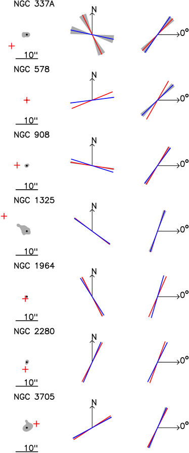
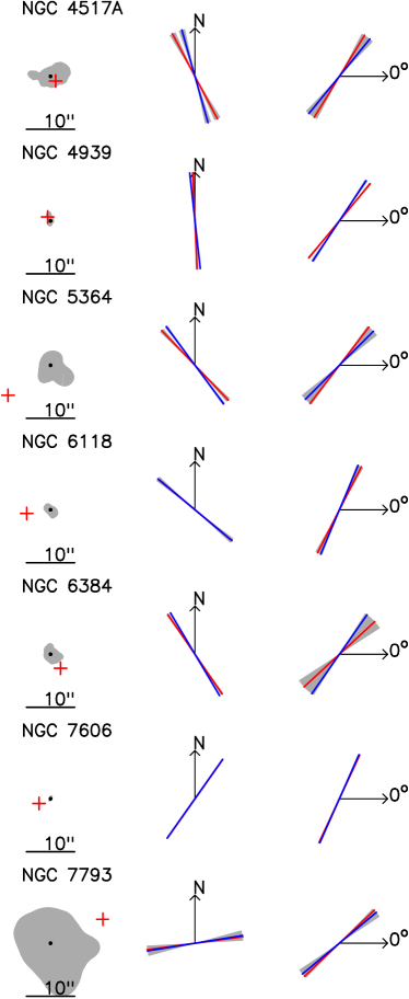
Figure 3.— Comparison between the projection geometry fitted to the kinematic map (blue) and the I-band photometric image (red). For each galaxy, the left-hand panel compares the fitted positions of the centers, with the shaded area showing the region that encloses 68% of the bootstrap estimates of the position of the best fit kinematic center, which is marked by the blue dot. The red plus symbol shows the location of the adopted photometric center on the same scale, for which there is no uncertainty estimate. Note that the center of NGC 578 was fixed at the photometric position when fitting the kinematic map. The fitted PA is shown in the middle panel and the inclination in the righthand panel, and again the gray shading indicates the 1-$\sigma$ uncertainties about the best fit value, which is less than the line width in some cases.

2.9.2 Migratory Image Artifacts

In our 28 Dec 2011 observations of NGC 908, NGC 1325, and NGC 2280 and our 29 Dec 2011 observation of NGC 578, we detect a series of bright objects which move coherently across our images. These objects have a different point spread function from that of the real objects in our images, and appear to be unfocused. In a time sequence of images, these objects move relative to the real objects of the field in a uniform way.

The relative abundance of these objects appears to be roughly proportional to the abundance of stars in each image, though we have been unable to register these objects with real stars. In the case of our 29 Dec 2011 observation of NGC 578, one of these objects is so bright that its diametric ghost (see §2.3) is visible and moves in the opposite direction to the other objects’ coherent movement.

Based on this information, we have arrived at a possible explanation for the appearance of these strange objects. We believe that on these two nights in Dec 2011, a small subset of SALT’s segmented primary mirror, perhaps only one segment, was misaligned with the rest of the primary mirror. This subset of the primary mirror then reflected out-of-field light into our field. As the secondary optics package moved through the focal plane to track our objects of interest, the stars reflected from outside the field then appear to move across the images due to the misalignment of this subset of mirror segments. New edge sensors have been installed between SALT’s primary mirror segments in the time since these observations were taken, so these types of image artifacts should not be present in future observations.

We have applied a simple mask over our images wherever these objects appear. Any pixels which fall within this mask are excluded from any calculations in the remainder of our data reduction process.

2.9.3 Other Image Artifacts

SALT utilizes a small probe to track a guide star over the course of an observation to maintain alignment with a target object. In some of our observations, the shadow of this guide probe overlaps our images (e.g. the lower right of the image in Figure 1). Similar to our treatment of the migrating objects above, we apply a mask over pixels which are affected by this shadow. We also apply such a mask in the rare cases in which a satellite trail overlaps our images.

3. Velocity and Intensity Maps

The results of the foregoing reductions of the raw data cube for each galaxy are 2D maps of median surface brightness, continuum surface brightness (i.e. $C$ from equation 4), integrated H$\alpha$ line surface brightness ($F_{H}$), integrated [N II] line surface brightness ($F_{N}$), line-of-sight velocity, and estimated uncertainty in velocity for each of our 14 galaxies. The total number of fitted pixels and number of independent resolution elements in each galaxy’s maps are summarized in Table 1.

3.1. Axisymmetric models and rotation curves

We have utilized the DiskFit software package (Spekkens & Sellwood, 2007; Sellwood & Zánmar Sánchez, 2010) to fit axisymmetric rotation models to our H$\alpha$ velocity fields. Unlike tilted-ring codes, e.g. rotcur (Begeman, 1987), DiskFit assumes a single projection geometry for the entire galactic disk and derives uncertainties on all the fitted parameters from a bootstrap procedure.

In addition to fitting for five global parameters, which mostly describe the projection geometry, it fits for a circular rotation speed in each of an arbitrary number of user-specified radius bins (i.e. the rotation curve). The five global parameters are: the position of the galaxy center ($x_{c},y_{c}$), the systemic recession velocity of the galaxy ($V_{\rm sys}$), the disk inclination ($i$), and the position angle of the disk relative to the North-South axis ($\phi_{\rm PA}$). For $N$ user-specified radius bins, DiskFit fits for the $N+5$ parameters using a $\chi^{2}$-minimization algorithm.

Where we have sufficiently dense velocity measurements, we typically space the $N$ radial bins along the major axis by 5″, which well exceeds the seeing in all cases, so that each velocity measurement is independent.

The velocity uncertainties used in calculating the $\chi^{2}$ values arise from two sources: the uncertainty in fitting a Voigt profile to each pixel’s spectrum (§2.8) and the intrinsic turbulence within a galaxy. This intrinsic turbulence, $\Delta_{\rm ISM}$, is in the range 7-12 km s^-1 both in the Milky Way (Gunn et al., 1979) and in external galaxies (Kamphuis, 1993). When most emission in a pixel arises from a single H II region, the measured velocity may differ from the mean orbital speed by some random amount drawn from this turbulent spread. We therefore add $\Delta_{\rm ISM}=12~{}$km s^-1 in quadrature to the estimated velocity uncertainty in each pixel when fitting these models to each of our galaxies.

We calculate uncertainties for each of these fitted parameters using the bootstrap method described in Sellwood & Zánmar Sánchez (2010). Due to the fact that these velocity maps can contain structure not accounted for in our models, residual velocities may be correlated over much larger regions than a single resolution element. To account for this, the bootstrap method preserves regions of correlated residual line of sight velocity when resampling the data to estimate the uncertainty values.

Table 2 lists the projection parameters and reduced-$\chi^{2}$ values for our best-fitting axisymmetric models to our 14 H$\alpha$ velocity maps. The uncertainty values in Table 2 and in the rotation curves of Figures 4-17 are the estimated 1-$\sigma$ uncertainties from 1000 bootstrap iterations. In some cases (e.g. NGC 7793), the inclination of the galaxy is poorly constrained in our axisymmetric models. This leads to a large uncertainty in the overall normalization of the rotation curve even when the shape of the rotation curve is well-constrained. This is the reason that uncertainties in the velocities are often substantially larger than the point-to-point scatter in the individual values.

3.2. Non-axisymmetric models

DiskFit is also capable of fitting more complicated models that include kinematic features such as bars, warped disks, and radial flows. We have attempted to fit our velocity maps with such models, but in no case have we obtained an improved fit that appeared convincing. Often a fitted “bar” was clearly misaligned with, and of different length from that visible in the galaxy image, and the bootstrap uncertainties yielded large errors on the fitted bar parameters. The DiskFit algorithm has been demonstrated to work well (Spekkens & Sellwood, 2007; Sellwood & Zánmar Sánchez, 2010) when there are well-determined velocities covering the region of the bar. But the DiskFit algorithm is unable to find a convincing fit when the velocity map lacks information at crucial azimuths of the expected bar flow, as appears to be the case for all the barred galaxies in our sample. This remains true even when the initial guesses at parameter values are chosen carefully. We therefore here present only axisymmetric fits to our data in which bars and other asymmetries are azimuthally averaged. We will discuss more complex kinematic models for these galaxies in future papers in this series.

3.3. Comparison with photometry

Kuzio de Naray et al. (in prep.) have applied the DiskFit package to multi-band photometric images of these galaxies, fitting both a disk and, where appropriate, a bulge and/or a bar. These fits yield the disk major axis position angle and an axis ratio that is interpreted as a measure of the inclination of a thin, round disk. In order to estimate color gradients, they fixed the photometric center in each image to the same sky position, and therefore did not obtain uncertainty estimates for the position of the center. Figure 3 presents a graphical comparison between the values derived separately from our kinematic maps and from the I-band image of each galaxy. In most cases, the measurements agree within the uncertainties. However, there are some significant differences. In particular, discrepancies in the fitted positions of the centers seem large compared with the uncertainties. In some cases, notably NGC 1325, NGC 3705, NGC 5364, NGC 6384, and NGC 7606, we have no kinematic measurements in the inner 15″ - 25″, which complicates fitting for the center. In all these cases, both the kinematic and photometric centers are well within the region where we have no kinematic data, while the radial extent of our maps is 10 - 20 times larger; forcing the kinematic center to coincide with the photometric center has little effect on the fitted inclination, position angle, and outer rotation curve. We discuss other cases in the following subsections about each galaxy

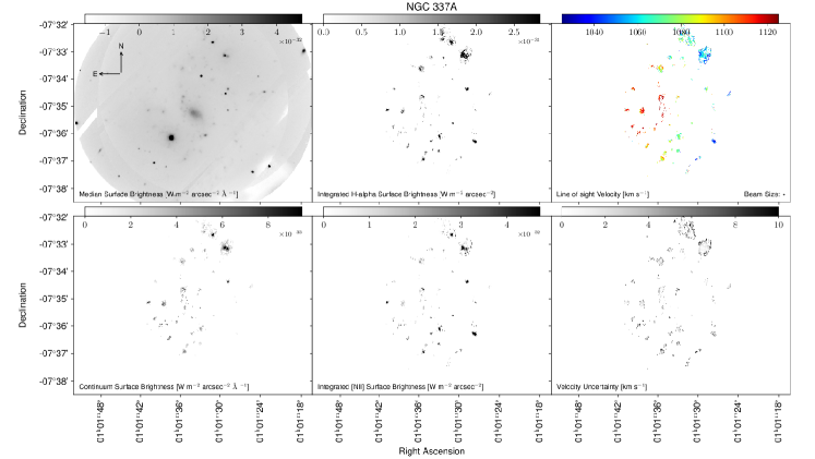
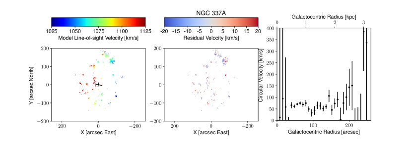
Figure 4.— Results for NGC 337A. Top left: the median flux for each pixel in our combined data cube. Middle left: the fitted continuum flux. Top center: the fitted integrated H$\alpha$ line flux. Middle center: the fitted integrated [N II] line flux. Top right: the fitted line-of-sight velocity. Middle right: the estimated uncertainty in the fitted line-of-sight velocity. At a distance of 2.57 Mpc, the physical scale is $12.5\textrm{ pc}/\arcsec$. Bottom left: Our best-fitting axisymmetric DiskFit model of NGC 337A’s line-of-sight H$\alpha$ velocity field. The center, orientation of the major axis, and axis-ratio of our best-fitting DiskFit model are marked with a large black cross. Bottom center: A map of the data-minus-model residual velocities for the best-fitting model in the left panel. Bottom right: A rotation curve extracted from the best-fitting axisymmetric model with 1-$\sigma$ uncertainties derived from our bootstrapping procedure. The radii were chosen to be at least 5″ apart, which is approximately 2 seeing elements.

4. Results for Individual Galaxies

4.1. NGC 337A

NGC 337A has one of the most sparsely sampled velocity maps in the RINGS medium-resolution H$\alpha$ kinematic data, as seen in Figure 4. It is also one of the two galaxies in this work (along with NGC 4517A) that are classified as Irregular. Despite this, our model is able to sample the rotation curve over a wide range of radii (Figure 4) extending out to $\sim 2.5~{}$kpc. Near the center and at $R\gtrsim 175$″, the velocity data are too sparse to yield a meaningful estimate of the circular speed.

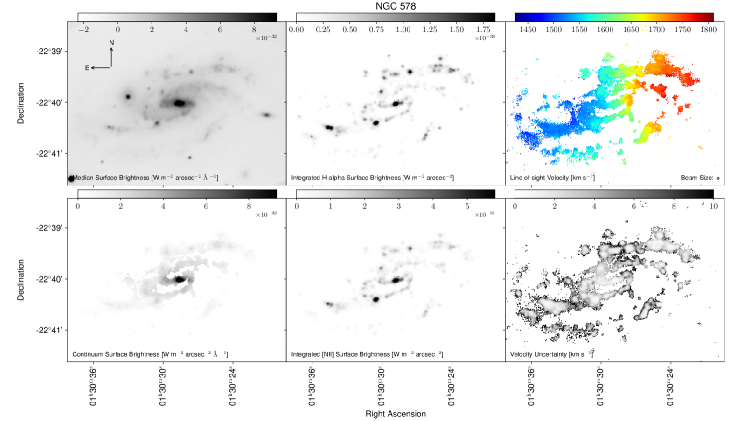
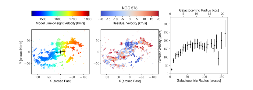
Figure 5.— Same as Figure 4, but for NGC 578. At a distance of 27.1 Mpc, the physical scale is $131\textrm{ pc}/\arcsec$. The large uncertainties on the points are due almost entirely to the galaxy’s inclination being poorly constrained.

Our best-fitting kinematic projection parameters for this galaxy differ substantially from those derived from the I-band image by Kuzio de Naray et al. (in prep.), as indicated in Figure 3, which is not too surprising given the sparseness of the kinematic map. In particular, the axis about which the galaxy is rotating appears to be strongly misaligned from the symmetry axis of the I-band light distribution. Since the kinematic data are clearly blueshifted on the West side of the galaxy and redshifted on the East, the misalignment is more probably due to difficulties in fitting the image; the light of NGC 337A is dominated by a bulge while the disk is very faint so that the apparent projection geometry of the galaxy is dominated by that of the bulge.

4.2. NGC 578

Even though NGC 578 exhibits one of the strongest visible bars among this sample of galaxies, we were disappointed to find that the velocity map (Figure 5) lacks sufficient data in the bar region to be able to separate a non-circular flow from the axisymmetric part. Note the absence of velocity information immediately to the N and S of the bar. We therefore derive an estimate of the rotation curve from an axisymmetric fit only. Also, for this galaxy only, we fix the center of rotation to the sky position of the photometric center. The coherent velocity features in the residual map clearly contain more information that we will examine more closely in a future paper in this series.

The slow, and almost continuous rise of the fitted circular speed affects our ability to determine the inclination of the disk plane to line of sight, which is generally more tightly constrained when the rotation curve has a clear peak. This galaxy therefore has one of the larger inclination uncertainties in the sample, which leads to the large uncertainties in the deprojection of the orbital speeds and to the fact that the point-to-point differences in the best fit values are substantially smaller than the uncertainties.

As shown in Figure 3, the best-fitting inclination and position angle for our kinematic models of this galaxy disagree significantly with the values derived from the photometric model of Kuzio de Naray et al. (in prep.), in which the bar was fitted separately. There are at least two reasons for this discrepancy: the prominent bar feature probably does affect the estimated projection geometry derived from an axisymmetric fit to the kinematic map and the galaxy image also manifests a strong asymmetry in the outer parts, with an unmatched spiral near the Northern minor axis, that complicates the fit to photometric image.

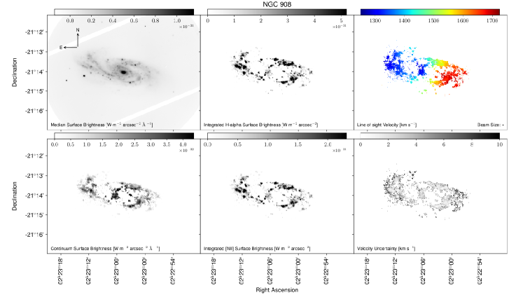
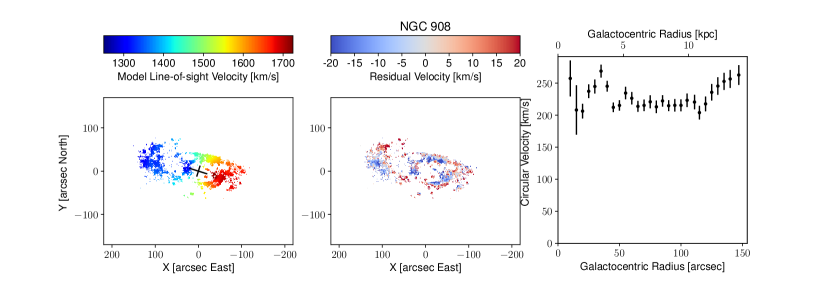
Figure 6.— Same as Figure 4, but for NGC 908. At a distance of 19.4 Mpc, the physical scale is $94.1\textrm{ pc}/\arcsec$.

In Figure 18, we compare our derived rotation curve with that reported by Mathewson & Ford (1996) via H$\alpha$ longslit spectroscopy (red points). There is generally somewhat smaller scatter in our points, and those authors adopt a higher inclination of 58°, compared with our 44°, causing them to derive circular speeds that are systematically lower by about 20%.

4.3. NGC 908

NGC 908 has a single large spiral arm towards the north-east side of the galaxy (see the top left panel of Figure 6) which is unmatched by a corresponding spiral arm on the opposite side. We have fitted an axisymmetric model, which therefore leads to a corresponding region of large correlated residual velocity. This feature is probably responsible for the sudden increase in the derived rotation curve beyond 120″, which could also be indicative of a warped disk at large radii.

Again, Figure 3 indicates that our best-fitting values for the center, position angle, and inclination of this galaxy differ somewhat from those fitted to the I-band image (Kuzio de Naray et al., in prep.), though this is not entirely surprising given the asymmetry of this galaxy.

As shown in Figure 18, the shape of our derived rotation curve for NGC 908 agrees fairly well with the previous long-slit measurements by Mathewson & Ford (1996), although we do not reproduce the slow inner rise that they report. Again they adopted a higher inclination of 66°, compared with our 54°, causing their circular speeds to be lower than ours by about 12%.

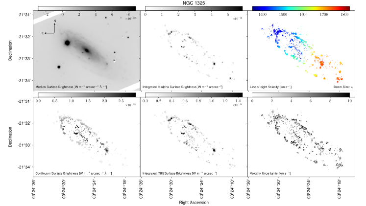
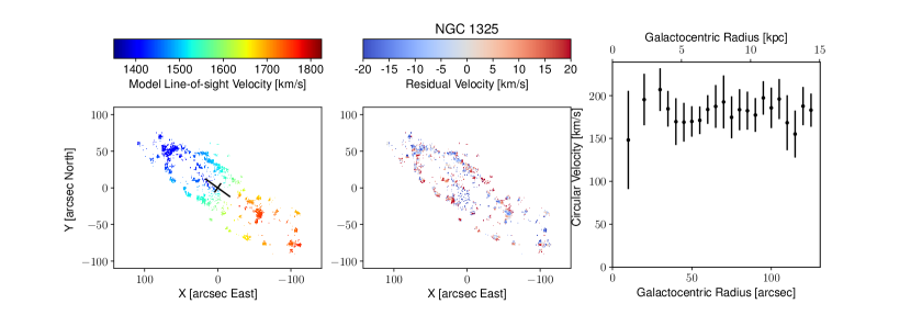
Figure 7.— Same as Figure 4, but for NGC 1325. At a distance of 23.7 Mpc, the physical scale is $115\textrm{ pc}/\arcsec$.

4.4. NGC 1325

Our data on NGC 1325 (Figure 7) indicate that this galaxy has a regular projected flow pattern. We derive a rotation curve that is approximately flat over a wide range of radii. Notably, we detect very little H$\alpha$ emission in the innermost $\sim 25$″ of the map, where our velocity estimates are correspondingly sparse and uncertain. Our best-fitting projection angles for this galaxy agree extremely well with those from the photometric models of Kuzio de Naray et al. (in prep.), as shown in Figure 3, but the position of the center differs by over 10″, probably because of the dearth of kinematic data in the inner parts.

Rubin et al. (1982) adopted an inclination of 70° for this galaxy, which is identical within the uncertainty with our best fit value, and our extracted rotation curve agrees reasonably well (Figure 18) with their measurements at $R>50\arcsec$. We do not, however, reproduce the slow rise interior to this radius that they report; this discrepancy could indicate that their slit did not pass through the center.

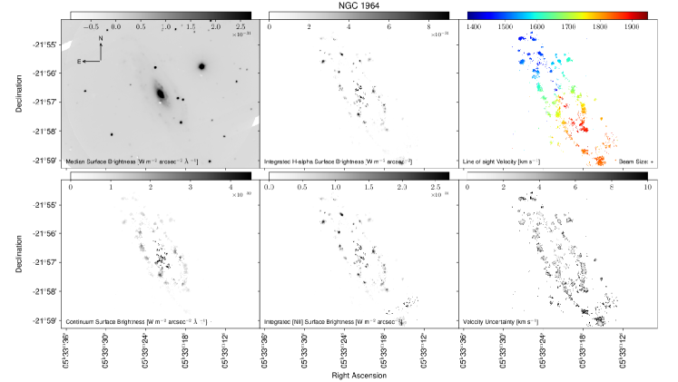
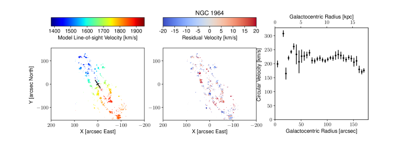
Figure 8.— Same as Figure 4, but for NGC 1964. At a distance of 20.9 Mpc, the physical scale is $101\textrm{ pc}/\arcsec$.

4.5. NGC 1964

We find, Figure 8, an almost regular flow pattern for NGC 1964. Our fitted center position and projection angles agree, within the estimated uncertainties (see Figure 3), with those derived from the I-band image by Kuzio de Naray et al. (in prep.).

As shown in Figure 18, our derived rotation curve is similar to that measured previously by Mathewson & Ford (1996), who adopted an inclination of 68°, compared to our 74°.

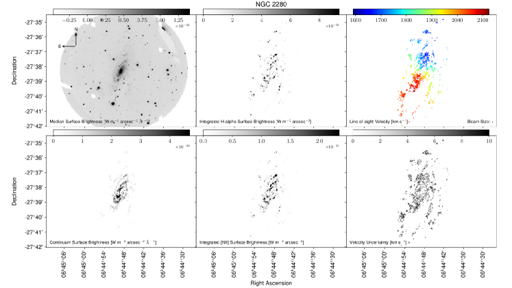
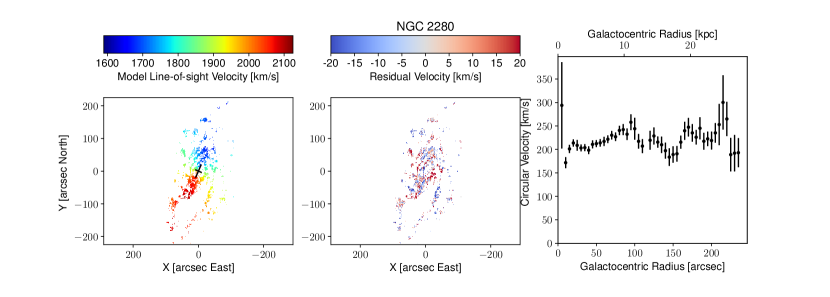
Figure 9.— Same as Figure 4, but for NGC 2280. At a distance of 24.0 Mpc, the physical scale is $116\textrm{ pc}/\arcsec$.

blah

4.6. NGC 2280

Our previous paper (Mitchell et al., 2015) presented a kinematic map for NGC 2280 that was derived from the same Fabry-Pérot data cube. The most significant difference between the maps and models presented in that work and those presented here is increased spatial resolution due to a change in our pixel binning procedure. As mentioned in §§2.2 and 2.3, we have made minor refinements to our flatfielding and ghost subtraction routines which have improved the data reduction process, and here we also include a fit to the [N II] 6583 line in addition to the H$\alpha$ line, which results in a slightly increased image depth.

Our derived velocity map for NGC 2280, presented in Figure 9, again reveals a regular flow pattern that is typical of a rotating disk galaxy seen in projection. Unlike many of the other galaxies in our sample, we have been able to extract reliable velocities at both very small and very large radii, producing one of the most complete rotation curves in this sample. Aside from the inermost point, which is very uncertain, the measured orbital speed agrees well with that in our previous paper, where we also demonstrated general agreeement with the H I rotation curve.

The position of the center, inclination, and position angle of this galaxy are very well constrained in our models, with uncertainties $\lesssim 1$° for both angle parameters. These values are consistent with our previous work on this galaxy in Mitchell et al. (2015), but the estimated inclination, 63.5° is in tension (see Figure 3) with the 69.6° derived from the I-band image by Kuzio de Naray et al. (in prep.), who also estimated the uncertainty on each angle to be $\sim 1\arcdeg$.

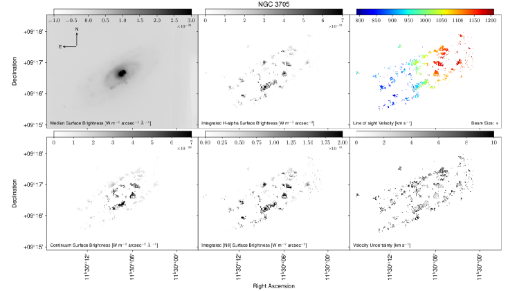
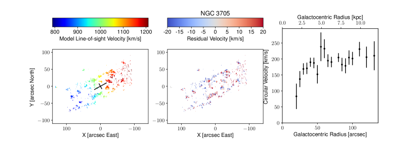
Figure 10.— Same as Figure 4, but for NGC 3705. At a distance of 18.5 Mpc, the physical scale is $89.7\textrm{ pc}/\arcsec$.

Our rotation curve NGC 2280 extends to much larger radii than those published previously, as shown in Figure 18. We derive systematically slightly larger velocities than did Mathewson & Ford (1996) (red points), who adopted $i=61\arcdeg$. Our estimated velocities are almost double the values reported by Sperandio et al. (1995) (green points), who did not give an inclination for this galaxy and may have reported projected, i.e. line-of-sight, velocities.

4.7. NGC 3705

We have derived the maps shown in Figure 10 from our data on NGC 3705. We detect no H$\alpha$ emission in the central $\sim 20\arcsec$ of the galaxy, and the innermost fitted velocities have large uncertainties. For $R\gtrsim 80\arcsec$, the rotation curve appears to be approximately flat over a broad range of radii.

Our values for NGC 3705’s center and projection angles are consistent with (see Figure 3) the values from the I-band image fitted by Kuzio de Naray et al. (in prep.), but our lack of velocity measurements at small radii made it difficult to pinpoint the center.

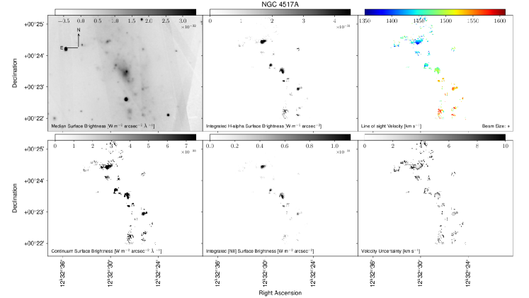
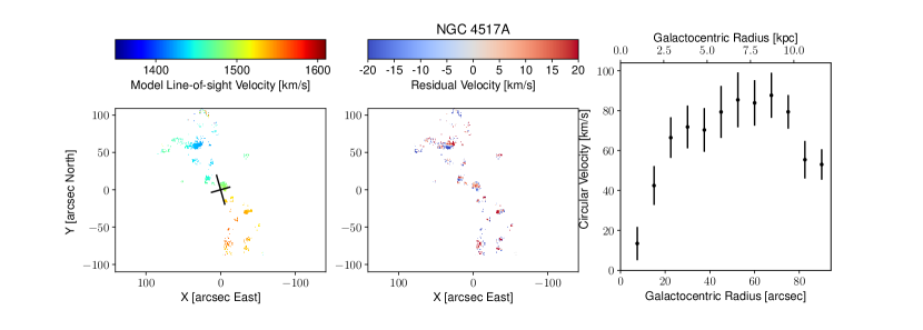
Figure 11.— Same as Figure 4, but for NGC 4517A. At a distance of 26.7 Mpc, the physical scale is $129\textrm{ pc}/\arcsec$.

blah

4.8. NGC 4517A

Our velocity map for NGC 4517A, Figure 11, like that for NGC 337A, is very sparsely sampled, and both galaxies are morphologically classified as Irregular. Our rotation curve extracted from an axisymmetric model of this galaxy is sparsely sampled and has large uncertainties. These uncertainties also reflect the uncertainty in the inclination.

The projection parameters of our best-fitting model have some of the largest uncertainties in Table 2, but are consistent, within the uncertainties (see Figure 3), with the values derived from the I-band image by Kuzio de Naray et al. (in prep.), and our fitted center agrees well with the photometric estimate.

Our estimates of the circular speed in NGC 4517A generally agree with the values measured by Neumayer et al. (2011), though both their PPAK data and ours are quite sparse (Figure 18). Their slightly higher orbital speeds are a consequence of a difference in adopted inclination of $i=90\arcdeg-33\arcdeg=57\arcdeg$ compared with our 51°.

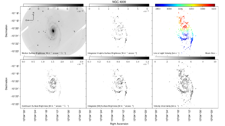
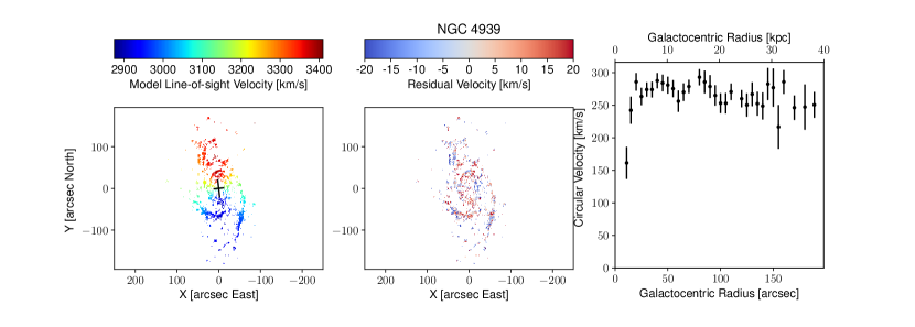
Figure 12.— Same as Figure 4, but for NGC 4939. At a distance of 41.6 Mpc, the physical scale is $202\textrm{ pc}/\arcsec$.

4.9. NGC 4939

Figure 12 presents our results for NGC 4939, which is the most luminous galaxy in our sample. The rotation curve rises steeply before becoming approximately flat for $R\gtrsim 25\arcsec$ at a value of 270 km s^-1 out to nearly 40 kpc in the disk plane. Our kinematic projection parameters and center for this galaxy agree very well (see Figure 3) with those derived from the I-band image by Kuzio de Naray et al. (in prep.).

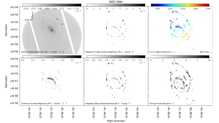
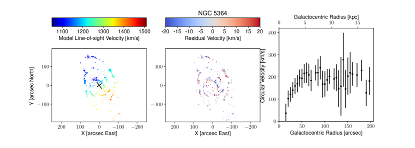
Figure 13.— Same as Figure 4, but for NGC 5364. At a distance of 18.1 Mpc, the physical scale is $87.8\textrm{ pc}/\arcsec$.

blah

4.10. NGC 5364

The H$\alpha$ emission in NGC 5364 very strongly traces its spiral arms and we detect no H$\alpha$ emission within the innermost $\sim 15\arcsec$. The rotation curve is rising roughly linearly outside this radius before becoming approximately flat for $R\gtrsim 80\arcsec$. Because the kinematic data are somewhat sparse, the galaxy’s inclination has a moderately large uncertainty, leading to a large uncertainty in the overall normalization of the rotation curve.

Our fitted position angle and inclination differ (see Figure 3) by a few degrees from the values derived from the I-band image by Kuzio de Naray et al. (in prep.), although differences are not large compared with the uncertainties. Again the lack of kinematic data in the inner part of map led to larger than usual uncertainties in the position of the center.

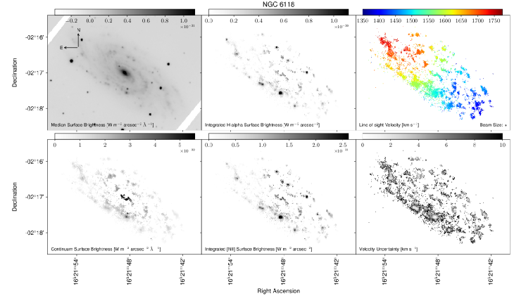
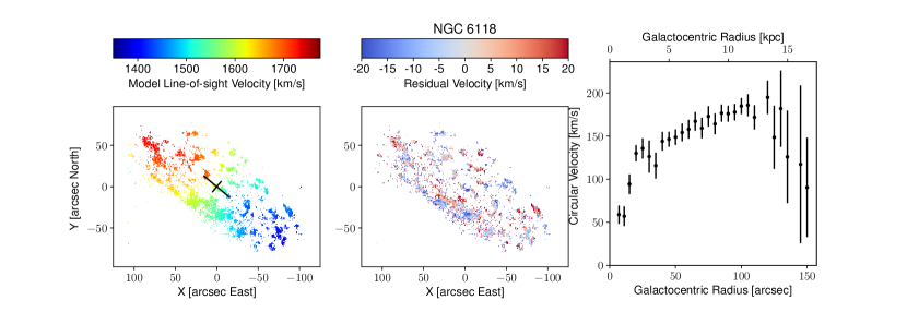
Figure 14.— Same as Figure 4, but for NGC 6118. At a distance of 22.9 Mpc, the physical scale is $111\textrm{ pc}/\arcsec$.

blah

4.11. NGC 6118

Our velocity map for NGC 6118 is presented in Figure 14. The rotation curve extracted from our axisymmetric model rises continuously from the center to $R\gtrsim 100\arcsec$. The decreasing values beyond this radius have large uncertainties.

Our best-fitting projection angles agree (Figure 3) with the values derived from the I-band image by Kuzio de Naray et al. (in prep.), but the centers disagree by about 5″, or about $6\sigma$.

Our rotation curve also agrees very well (Figure 18) with that obtained by Meyssonnier (1984) using a longslit and who adopted an inclination of 62°.

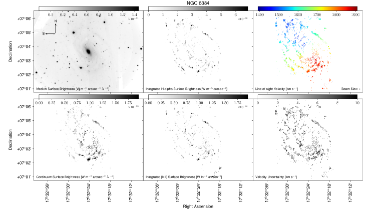
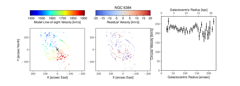
Figure 15.— Same as Figure 4, but for NGC 6384. At a distance of 19.7 Mpc, the physical scale is $95.5\textrm{ pc}/\arcsec$.

blah

4.12. NGC 6384

We present our velocity map for NGC 6384 in Figure 15. As in NGC 5364, the H$\alpha$ emission closely traces the spiral arms. We detect no H$\alpha$ emission within the innermost $\sim 25\arcsec$. Our fitted rotation curve is roughly flat from this point to the outermost limits of our data.

Our best-fitting model’s inclination is in reasonable agreement with the uncertain value (see Figure 3) derived from the I-band image by Kuzio de Naray et al. (in prep.), while the position angle and center are in better agreement.

Figure 18 shows that our estimates of the circular speed in NGC 6384 are systematically higher than those of Sperandio et al. (1995), as was the case for NGC 2280. Again these authors appear not have corrected their orbital speeds for inclination.

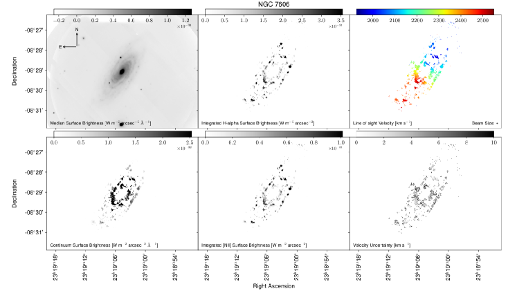
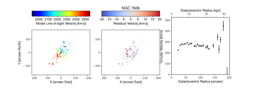
Figure 16.— Same as Figure 4, but for NGC 7606. At a distance of 34.0 Mpc, the physical scale is $165\textrm{ pc}/\arcsec$.

blah

4.13. NGC 7606

NGC 7606 is the fastest-rotating galaxy in this sample and the second most-luminous. Again the velocity map, Figure 16, displays the flow pattern of a typical spiral disk, and again we detect no H$\alpha$ emission in the innermost $\sim 15\arcsec$. Our fitted rotation curve appears to be rising from our innermost point, becoming roughly flat from $R\sim 30\arcsec$, before declining somewhat from $\sim 50$–$120\arcsec$ with a hint of an outer increase, although the uncertainties are large due to the sparseness of our data at these radii.

The inclination and position angle of this galaxy are extremely tightly constrained by our kinematic models and agree very well, Figure 3, with the projection angles derived from the I-band image by Kuzio de Naray et al. (in prep.), as does the location of the center despite the absence of data at small radii.

In general, our rotation curve measurements agree well with the previous measurements by Rubin et al. (1982) (blue points in Figure 18) and Mathewson & Ford (1996) (red points), who adopted inclinations of 66° and 70° respectively.

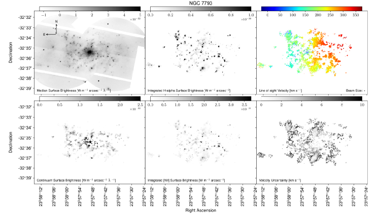
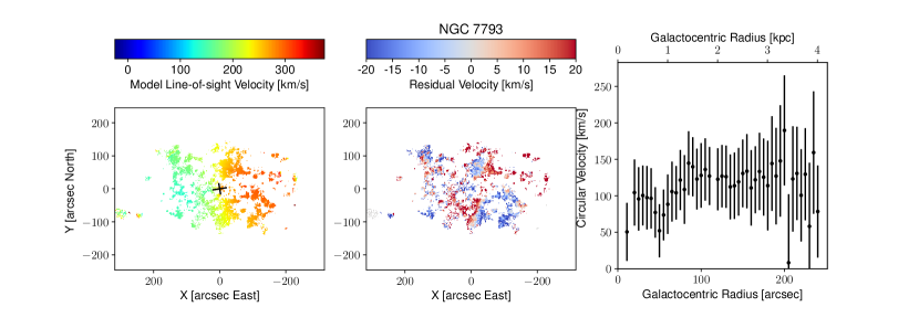
Figure 17.— Same as Figure 4, but for NGC 7793. At a distance of 3.44 Mpc, the physical scale is $16.7\textrm{ pc}/\arcsec$. Because we obtained 4 observations of the East (approaching) side of this galaxy and only 1 observation of the West (receding) side, our sensitivity is significantly stronger on the Eastern portion of these maps. All 5 observations overlap in the central region.

4.14. NGC 7793

NGC 7793 has the largest angular size of our sample and the velocity map, Figure 17, was derived from the combination of two separate pointings.

Our fitted rotation curve shows a general rise to $R\sim 100\arcsec$, except for a slight decrease around $R\sim 40\arcsec$. Our data in the outermost parts of the galaxy are too sparse to measure the orbital speed reliably. As for NGC 337A, the large uncertainties on individual points in the rotation curve are mostly due to the large uncertainty in NGC 7793’s inclination in our model.

The projection parameters of our best-fitting model agree well within the larger than usual uncertainties, Figure 3, with those derived from the I-band image by Kuzio de Naray et al. (in prep.), and while our fitted center is some 14″ from the photometric center, our uncertainty estimates are also large, so that this discrepancy is $2.5\sigma$.

Again in Figure 18 we compare our estimated rotation curve with those previously reported by Davoust & de Vaucouleurs (1980) (orange points) and by Dicaire et al. (2008) (purple points), who adopted inclinations of 53° and 46° respectively that are both larger than our 40°. Consequently, our estimated speeds are above theirs at most radii. The shapes of the rotation curves are generally similar, although we find a steeper inner rise.

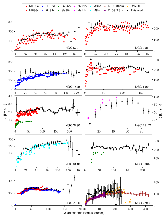
Figure 18.— A comparison of our best-fitting model rotation curves (black circles with error bars) to previous measurements from the literature. In all cases, squares are from the approaching side of the galaxy, triangles from the receding side, and circles from an azimuthal average. Unless otherwise specified, we have used own own best-fitting values for systemic velocity and inclination (see Table 2) to deproject the data. Red points (NGC 578, 908, 1964, 2280, and 7606): Mathewson & Ford (1996) via H$\alpha$ longslit spectroscopy (Note: We have adopted a systemic velocity of 1960 km s^-1 for NGC 1964 rather than our best-fitting value to match the authors’ spectra. The authors also report a rotation curve for NGC 1325, but the wavelength calibration for those data appears to have been incorrect.). Blue points (NGC 1325 and 7606): Rubin et al. (1982) via H$\alpha$ and [N II] longslit spectroscopy. Green points (NGC 2280 and 6384): Sperandio et al. (1995) via H$\alpha$ and [N II] longslit spectroscopy. Magenta points (NGC 4517A): Neumayer et al. (2011) via H$\alpha$ IFU spectroscopy. Cyan points (NGC 6118): Meyssonnier (1984) via optical longslit spectroscopy. Brown and purple points (NGC 7793): Dicaire et al. (2008) via H$\alpha$ Fabry-Pérot spectrophotometry. Orange points (NGC 7793): Davoust & de Vaucouleurs (1980) via H$\alpha$ Fabry-Pérot spectrophotometry.

4.15. Discussion

As we have discussed for the individual cases, the rotation curves we derive from fitting axisymmetric flow patterns to our velocity maps agree quite well with previously published estimates from several different authors and using a number of different optical instruments. These comparisons are shown in Figure 18, where most systematic discrepancies can be attributed to differences between the inclinations we adopt, and those in the comparison work. This generally good agreement is reassuring.

4.16. Oval disks?

Discrepancies between the position angle and inclination fitted separately to a kinematic map and a photometric image of the same galaxy would be expected if the disk were intrinsically oval, as has been claimed in some cases (e.g Portas et al., 2011) and emphasized as a possibility by Kormendy (2013). Even were the projected major axis to be closely aligned with either of the principal axes of a strongly oval disk, the fitted inclinations should differ.

We have no clear evidence of this behavior in our sample of galaxies, since the projection angles derived from fitting axisymmetric models to our velocity maps generally agree, within the estimated uncertainties, with those fitted to the I-band images (Kuzio de Naray et al., in prep.), as shown in Figure 3. We argued above that the discrepancy in NGC 337A is due to the faintness of the outer disk, while those in NGC 578 and NGC 908 can be ascribed to asymmetries. Note that Barnes & Sellwood (2003) reported that the position angle of the galaxy major axis estimated from photometric images and kinematic maps never exceeded 4° in their larger sample of 74 galaxies, and Barrera-Ballesteros et al. (2014) found only minor misalignments in a sample of intrinsically barred galaxies. Since these were all randomly selected spiral galaxies, it would seem that the incidence of intrinsically oval disks is low, at least over the radial extent of these maps.

Futhermore, Barnes & Sellwood (2003), found that the kinematic centers of their models were within 2$\farcs$7 of the photmetric centers in 67 out of 74 galaxies in their sample. Here we find the centers of our kinematic models are consistent in several cases with the photometric centers (see Figure 3), and the greater discrepancies generally arise where our maps are sparse or lack data in the center.

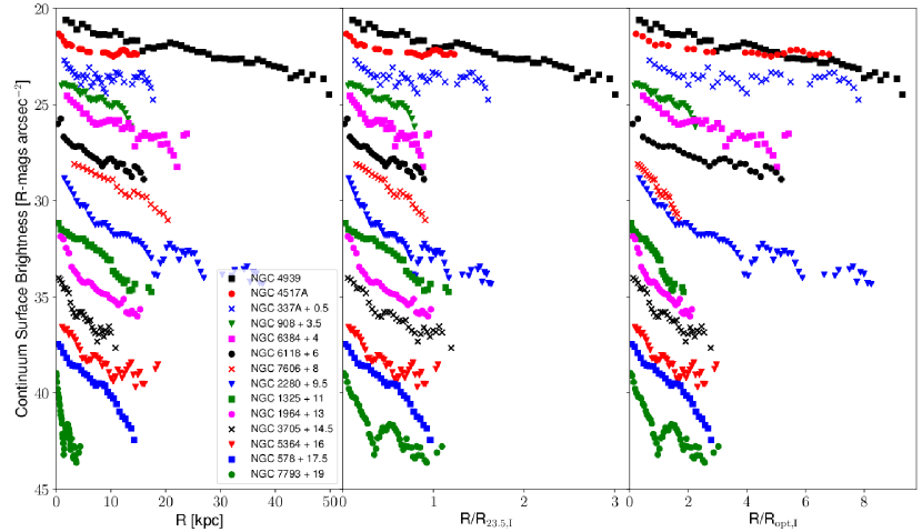
Figure 19.— Left: Azimuthally averaged R-band continuum surface brightness profiles plotted as functions of galactocentric radius in kpc. Center: The same values plotted as functions of galactocentric radius rescaled by each galaxy’s $R_{23.5}$ in the I-band. Right: The same values plotted as functions of galactocentric radius rescaled by each galaxy’s $R_{\rm opt}$ in the I-band. In each panel, the lines have been vertically offset by a constant to separate them.

5. Radial trends

Figure 19 shows the azimuthally averaged R-band continuum surface brightness of our galaxies derived from our H$\alpha$ Fabry-Pérot data cubes plotted against three different measures of galactocentric radius. These surface brightness profiles assume that the disk projection parameters are those of the best-fitting I-band models of Kuzio de Naray et al. (in prep.). The surface brightness profiles show qualitative and quantitative agreement with the R-band surface brightness profiles of Kuzio de Naray et al. (in prep.), but have a smaller radial extent.

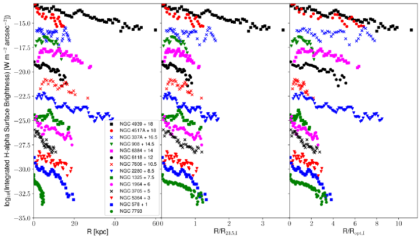
Figure 20.— Left: Azimuthally averaged integrated H$\alpha$ surface brightness profiles plotted as functions of galactocentric radius in kpc. Center: The same values plotted as functions of galactocentric radius rescaled by each galaxy’s $R_{23.5}$ in the I-band. Right: The same values plotted as functions of galactocentric radius rescaled by each galaxy’s $R_{\rm opt}$ in the I-band. In each panel, the lines have been vertically offset by a constant to separate them.

Figure 20 shows the azimuthally averaged integrated H$\alpha$ surface brightnesses of our galaxies, i.e. the values of $F_{H}$ in Equation 4. These values should be considered as lower limits on the true H$\alpha$ intensity, as the averages were taken over all pixels in a radial bin, including those which fell below our signal-to-noise threshold.

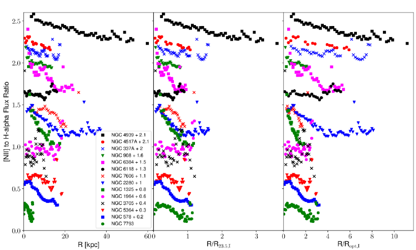
Figure 21.— Left: Azimuthally averaged N2 Index ($\mathrm{N2}\equiv\log(\mathrm{F_{\mathrm{N2~{}6583}}/\mathrm{F_{H\alpha}}})$) plotted as functions of galactocentric radius in kpc. Center: The same values plotted as functions of galactocentric radius rescaled by each galaxy’s $R_{23.5}$ in the I-band. Right: The same values plotted as functions of galactocentric radius rescaled by each galaxy’s $R_{\rm opt}$ in the I-band. In each panel, the lines have been vertically offset by a constant to separate them.

5.1. [N II]-to-H$\alpha$ Ratio and Oxygen Abundance

Figure 21 shows the azimuthally averaged value of the ratio of the integrated [N II] 6583 surface brightness to the integrated H$\alpha$ surface brightness, commonly known as the “N2 Index” (Alloin et al., 1979)

$$\mathrm{N2}\equiv\log(F_{\mathrm{N2}~{}6583}/F_{\mathrm{H\alpha}}).$$ (6)

It is important to note that the plotted quantity is the average value of the ratio ($\langle F_{N}/F_{H}\rangle$) and not the ratio of the averages ($\langle F_{N}\rangle/\langle F_{H}\rangle$). We note that all of our galaxies show a downward trend in this parameter. The relative intensities of these two lines are complicated functions of metallicity and electron temperature in the emitting gas, and the line intensity ratio is also known to be sensitive to the degree of ionization of the gas (Shaver et al., 1983).

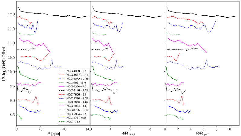
Figure 22.— Left: Azimuthally averaged oxygen abundances ($12+\log(\mathrm{O}/\mathrm{H})$) plotted as functions of galactocentric radius in kpc. Center: The same values plotted as functions of galactocentric radius rescaled by each galaxy’s $R_{23.5}$ in the I-band. Right: The same values plotted as functions of galactocentric radius rescaled by each galaxy’s $R_{\rm opt}$ in the I-band. In each panel, the lines have been vertically offset by a constant to separate them.

Because this ratio is sensitive to the metallicity of a galaxy and does not strongly depend on absorption, it has been widely used as an indicator of oxygen abundance (e.g. Pérez-Montero & Contini, 2009; Marino et al., 2013); Pettini & Pagel (2004) show that the data support an approximately linear relation between oxygen abundance and N2 index, which holds over the range $-2\gtrsim\mathrm{N2}\gtrsim-0.5$, but the relation may steepen at both higher and lower values of the ratio. Marino et al. (2013) give the following relation between the N2 index and oxygen abundance:

$$12+\log(\mathrm{O}/\mathrm{H})=8.743+0.462\times\mathrm{N2}.$$ (7)

We have used this relation to derive the mean radial variation of oxygen abundance in our galaxies displayed in Figure 22. As in many previous studies, we find that our galaxies generally manifest a declining trend in metallicity (e.g. Vila-Costas & Edmunds, 1992; Zaritsky et al., 1994; Moustakas et al., 2010; Belfiore et al., 2017). With the exception of NGC 6384, the most extended normalized profiles (e.g. NGC 4939, NGC 337A, NGC 4939, NGC 2280) show hints of a flattening in the outer parts, as has also been reported for large samples (e.g. Sánchez et al., 2014; Sánchez-Menguiano et al., 2016). NGC 4939 is the only galaxy discussed in this work known to host an active galactic nucleus (AGN). Away from the nucleus of this galaxy, and in all other galaxies in our sample, most ionizing radiation probably comes from hot, young stars. The extra ionizing radiation from the AGN in NGC 4939 may be the reason for central spike in the apparent oxygen abundance in this case.

6. Summary

We have presented high spatial resolution ($\sim$2.5″) H$\alpha$ velocity fields of 14 of the 19 galaxies in the RINGS sample, as well as maps of these galaxies’ R-band continuum emission and H$\alpha$ and [N II] integrated surface brightness. Additionally, we have presented azimuthally averaged integrated surface brightness profiles of these emission lines. We observe a general downward trend of the [N II]-to-H$\alpha$ emission ratio with radius in all of our galaxies.

We have used the DiskFit software package of Spekkens & Sellwood (2007) and Sellwood & Zánmar Sánchez (2010) to model the velocity fields presented in this work. From these models, we have extracted rotation curves at high spatial resolution and have shown good general agreement with those previously published, where available. In most cases, the projection geometries of these models agree well with the photometric models of Kuzio de Naray et al. (in prep.). This agreement argues against the disks being intrinsically oval.

As of 2015 Sept, the medium-resolution Fabry-Pérot etalon of SALT RSS is no longer available for observations due to deterioration of the reflective coatings. The remaining five galaxies of the RINGS sample are scheduled to be completed in the Fabry-Pérot system’s high-resolution mode.

References

- Alloin et al. (1979) Alloin, D., Collin-Souffrin, S., Joly, M., & Vigroux, L. 1979, A&A, 78, 200
- Astropy Collaboration et al. (2013) Astropy Collaboration, Robitaille, T. P., Tollerud, E. J., et al. 2013, A&A, 558, A33
- Barnes & Sellwood (2003) Barnes, E. I., & Sellwood, J. A. 2003, AJ, 125, 1164
- Barrera-Ballesteros et al. (2014) Barrera-Ballesteros, J. K., Falcón-Barroso, J., García-Lorenzo, B., et al. 2014, A&A, 568, A70
- Begeman (1987) Begeman, K. G. 1987, PhD thesis, , Kapteyn Institute, (1987)
- Belfiore et al. (2017) Belfiore, F., Maiolino, R., Tremonti, C., et al. 2017, MNRAS, 469, 151
- Bershady et al. (2010) Bershady, M. A., Verheijen, M. A. W., Swaters, R. A., et al. 2010, ApJ, 716, 198
- Bosma (1978) Bosma, A. 1978, PhD thesis, PhD Thesis, Groningen Univ., (1978)
- Bottinelli et al. (1985) Bottinelli, L., Gouguenheim, L., Paturel, G., & de Vaucouleurs, G. 1985, A&AS, 59, 43
- Brook (2015) Brook, C. B. 2015, MNRAS, 454, 1719
- Brook et al. (2011) Brook, C. B., Governato, F., Roškar, R., et al. 2011, MNRAS, 415, 1051
- Cappellari & Copin (2003) Cappellari, M., & Copin, Y. 2003, MNRAS, 342, 345
- Crawford et al. (2010) Crawford, S. M., Still, M., Schellart, P., et al. 2010, in Proc. SPIE, Vol. 7737, Observatory Operations: Strategies, Processes, and Systems III, 773725
- Davoust & de Vaucouleurs (1980) Davoust, E., & de Vaucouleurs, G. 1980, ApJ, 242, 30
- Di Cintio et al. (2014) Di Cintio, A., Brook, C. B., Macciò, A. V., et al. 2014, MNRAS, 437, 415
- Dicaire et al. (2008) Dicaire, I., Carignan, C., Amram, P., et al. 2008, AJ, 135, 2038
- Einasto (1965) Einasto, J. 1965, Trudy Astrofizicheskogo Instituta Alma-Ata, 5, 87
- Epinat et al. (2008) Epinat, B., Amram, P., Marcelin, M., et al. 2008, MNRAS, 388, 500
- Erroz-Ferrer et al. (2015) Erroz-Ferrer, S., Knapen, J. H., Leaman, R., et al. 2015, MNRAS, 451, 1004
- Gao et al. (2008) Gao, L., Navarro, J. F., Cole, S., et al. 2008, MNRAS, 387, 536
- Gnedin et al. (2004) Gnedin, O. Y., Kravtsov, A. V., Klypin, A. A., & Nagai, D. 2004, ApJ, 616, 16
- Governato et al. (2010) Governato, F., Brook, C., Mayer, L., et al. 2010, Nature, 463, 203
- Gunn et al. (1979) Gunn, J. E., Knapp, G. R., & Tremaine, S. D. 1979, AJ, 84, 1181
- Hayashi & Navarro (2006) Hayashi, E., & Navarro, J. F. 2006, MNRAS, 373, 1117
- Herbig (1995) Herbig, G. H. 1995, ARA&A, 33, 19
- Hernandez et al. (2005) Hernandez, O., Carignan, C., Amram, P., Chemin, L., & Daigle, O. 2005, MNRAS, 360, 1201
- Hernandez et al. (2008) Hernandez, O., Fathi, K., Carignan, C., et al. 2008, PASP, 120, 665
- Holmes et al. (2015) Holmes, L., Spekkens, K., Sánchez, S. F., et al. 2015, MNRAS, 451, 4397
- Humlíček (1982) Humlíček, J. 1982, Journal of Quantitative Spectroscopy and Radiative Transfer, 27, 437
- Hunter (2007) Hunter, J. D. 2007, Computing In Science & Engineering, 9, 90
- Jones et al. (2002) Jones, D. H., Shopbell, P. L., & Bland-Hawthorn, J. 2002, MNRAS, 329, 759
- Jones et al. (2001) Jones, E., Oliphant, T., Peterson, P., et al. 2001, SciPy: Open source scientific tools for Python
- Kamphuis (1993) Kamphuis, J. J. 1993, PhD thesis, PhD Thesis, University of Groningen, (1993)
- Katz et al. (2017) Katz, H., Lelli, F., McGaugh, S. S., et al. 2017, MNRAS, 466, 1648
- Kormendy (2013) Kormendy, J. 2013, Secular Evolution in Disk Galaxies, ed. J. Falcón-Barroso & J. H. Knapen, 1