Effects of finite-range interactions on the one-electron spectral properties of one-dimensional metals: Application to Bi/InSb(001)
Abstract
We study the one-electron spectral properties of one-dimensional interacting electron systems in which the interactions have finite range. We employ a mobile quantum impurity scheme that describes the interactions of the fractionalized excitations at energies above the standard Tomonga-Luttinger liquid limit and show that the phase shifts induced by the impurity describe universal properties of the one-particle spectral function. We find the explicit forms in terms of these phase shifts for the momentum dependent exponents that control the behavior of the spectral function near and at the -plane singularities where most of the spectral weight is located. The universality arises because the line shape near the singularities is independent of the short-distance part of the interaction potentials. For the class of potentials considered here, the charge fractionalized particles have screened Coulomb interactions that decay with a power-law exponent . We apply the theory to the angle-resolved photo-electron spectroscopy (ARPES) in the highly one-dimensional bismuth-induced anisotropic structure on indium antimonide Bi/InSb(001). Our theoretical predictions agree quantitatively with both (i) the experimental value found in Bi/InSb(001) for the exponent that controls the suppression of the density of states at very small excitation energy and (ii) the location in the plane of the experimentally observed high-energy peaks in the ARPES momentum and energy distributions. We conclude with a discussion of experimental properties beyond the range of our present theoretical framework and further open questions regarding the one-electron spectral properties of Bi/InSb(001).
I Introduction
One-dimensional (1D) interacting systems are characterized by a breakdown of the basic Fermi liquid quasiparticle picture. Indeed, no quasiparticles with the same quantum numbers as the electrons exist when the motion is restricted to a single spatial dimension. Rather, in a 1D lattice, correlated electrons split into basic fractionalized charge-only and spin-only particles Blumenstein_11 ; Voit_95 . Hence the removal or addition of electrons generates an energy continuum of excitations described by these exotic fractionalized particles which are not adiabatically connected to free electrons. Hence they must be described using a different language.
These models share common low-energy properties associated with the universal class of the Tomonaga-Luttinger liquid (TLL) Blumenstein_11 ; Voit_95 ; Tomonaga_50 ; Luttinger_63 . To access their high-energy dynamical correlation functions beyond the low-energy TLL limit, approaches such as the pseudofermion dynamical theory (PDT) Carmelo_05 or the mobile quantum impurity model (MQIM) Imambekov_09 ; Imambekov_12 must be used. Those approaches incorporate nonlinearities in the dispersion relations of the fractionalized particles.
An important low-energy TLL property of 1D correlated electronic metallic systems is the universal power-law scaling of the spectral intensity such that and . Here the exponent controls the suppression of the density of states (SDS) and is a small excitation energy near the ground-state level. The value SDS exponent is determined by that of the TLL charge parameter Blumenstein_11 ; Voit_95 ; Schulz_90 . Importantly, this exponent provides useful information about the range of the underlying electron interactions.
In the case of integrable 1D models solvable by the Bethe ansatz Bethe_31 (such as the 1D Hubbard model Lieb_68 ; Martins_98 ), the PDT and MQIM describe the same mechanisms and lead to the same expressions for the dynamical correlation functions Carmelo_18 . The advantage of the MQIM is that it also applies to non-integrable systems Imambekov_12 . The exponents characterizing the singularities in these systems differ significantly from the predictions of the linear TLL theory, except in the low-energy limit where the latter is valid.
For integrable 1D lattice electronic models with only onsite repulsion (such as the Hubbard model), the TLL charge parameter is larger than and thus the SDS exponent is smaller than . In non-integrable systems a SDS exponent larger than stems from finite-range interactions Schulz_90 .
In fact, as shown in Table 1, for the metallic states of both 1D and quasi-1D electronic systems, the SDS exponent frequently has experimental values in the range Blumenstein_11 ; Voit_95 ; Schulz_90 ; Claessen_02 ; Kim_06 ; Schoenhammer_93 ; Ma_17 ; Ohtsubo_15 ; Ohtsubo_17 . In actual materials, a finite effective range interaction Bethe_49 ; Blatt_49 ; Joachain_75 ; Preston_75 ; Flambaum_99 generally results from screened long-range Coulomb interactions with potentials vanishing as an inverse power of the separation with an exponent larger than one. In general, such finite-range interactions in 1D lattice systems represent a complex and unsolved quantum problem involving non-perturbative microscopic electronic processes. Indeed, as originally formulated, the MQIM does not apply to lattice electronic systems with finite-range interactions whose screened Coulomb potentials vanish as an inverse power of the electron distance.
Recently, the MQIM has been extended to a class of electronic systems with effective interaction ranges of about one lattice spacing, compatible with the high-energy one-electron spectral properties observed in twin grain boundaries of molybdenum diselenide MoSe2 Ma_17 ; Cadez_19 . This has been achieved by suitable renormalization of the phase shifts of the charge fractionalized particles. That theoretical scheme, called here “MQIM-LO”, accounts for the effects of only the leading order (LO) in the effective range expansion Bethe_49 ; Blatt_49 of such phase shifts.
In this paper we consider a bismuth-induced anisotropic structure on indium antimonide which we henceforth call Bi/InSb(001) Ohtsubo_15 . Experimentally, strong evidence has been found that Bi/InSb(001) exhibits 1D physics Ohtsubo_15 ; Ohtsubo_17 . However, a detailed understanding of the exotic one-electron spectral properties revealed by its angle resolved photo-emission spectroscopy (ARPES) Ohtsubo_15 ; Ohtsubo_17 at energy scales beyond the TLL has remained elusive. In particular, the predictions of the MQIM-LO for the location in the plane of the experimentally observed high-energy peaks in the ARPES momentum distribution curves (MDC) and energy distribution curves (EDC) of Bi/InSb(001) do not lead to the same quantitative agreement as for the ARPES in the MoSe2 line defects Ma_17 ; Cadez_19 . This raises the important question of what additional effects must be included to obtain agreement with the experimental data.
In this paper, we answer this question by extending the MQIM-LO to a larger class of 1D lattice electronic systems with finite-range interactions by accounting for higher-order terms in the effective range expansion Bethe_49 ; Blatt_49 ; Landau_65 ; Kermode_90 ; Burke_11 of the phase shifts of the fractionalized charged particles. While the corresponding higher order “MQIM-HO” corresponds in general to a complicated, non-perturbative many-electron problem, we find, unexpectedly, that the interactions of the fractionalized charged particles with the charge mobile quantum impurity occur in the unitary limit of (minus) infinite scattering length Newton_82 ; Zwerger_12 ; Horikoshi_17 . In that limit, the separation between the interacting charged particles (the inverse density) is much greater than the range of the interactions, and the calculations simplify considerably.
The unitary limit plays an important role in the physics of many physical systems, including the dilute neutron matter in shells of neutron stars Dean_03 and in atomic scattering in systems of trapped cold atoms Zwerger_12 ; Horikoshi_17 . Our discovery of its relevance in a condensed matter system is new and reveals new physics.
| System | Parameter | SDS exponent | Technique | Source |
|---|---|---|---|---|
| (TMTSF)2XX=PF6,AsF6,ClO4 | Optical conductivity | from SI of Ref. Blumenstein_11, | ||
| Carbon Nanotubes | Photoemission | from SI of Ref. Blumenstein_11, | ||
| Purple Bronze Li0.9Mo6O17 | ARPES and tunneling spectroscopy | from SI of Ref. Blumenstein_11, | ||
| 1D Gated Semiconductors | Transport conductivity | from SI of Ref. Blumenstein_11, | ||
| MoSe2 1D line defects | ARPES | from Ref. Ma_17, | ||
| Bi/InSb(001) | ARPES | from Ref. Ohtsubo_15, |
The results of the MQIM-HO are consistent with the expectation that the microscopic mechanisms behind the one-electron spectral properties of Bi/InSb(001) include finite-range interactions. Indeed, accounting for the effective range of the corresponding interactions Joachain_75 ; Preston_75 ; Flambaum_99 leads to theoretical predictions that quantitatively agree with both (i) the experimental value of the SDS exponent () in Bi/InSb(001) observed in and (ii) the location in the plane of the experimentally observed high-energy peaks in the ARPES MDC and EDC.
Since Bi/InSb(001) is a complex system and the MQIM-HO predictions are limited to the properties (i) and (ii), in the discussion section of this paper we consider other possible effects beyond the present theoretical framework that might contribute to the microscopic mechanisms determining spectral properties of Bi/InSb(001).
In this paper we employ units of and . In Sec. II we introduce the theoretical scheme used in our studies. The effective-range expansion of the phase shift associated with the interactions of the charge fractionalized particles and charge hole mobile impurity, the corresponding unitary limit, and the scattering lengths are all issues we address in Sec. III. In Sec. IV the effective range expression is derived and expressed in terms of the ratio of the renormalized and bare scattering lengths. In Sec. V we show how our approach predicts the location in the plane of the experimentally observed high-energy Bi/InSb(001) ARPES MDC and EDC peaks. In Sec. VI, we discuss our results and experimental properties outside the present theoretical framework, mention open questions on the Bi/InSb(001) spectral properties, and offer concluding remarks.
II The model
The 1D model Hamiltonian associated with the MQIM-HO for electronic density is given by,
| (1) |
Here , , for , and is a continuous screening function such that , which at large vanishes as some inverse power of whose exponent is larger than one, so that .
We use a representation of the fractionalized (charge) and (spin) particles that also naturally emerges in the MQIM-LO Ma_17 . For simplicity, in general in this paper they are called particles and particles, respectively. They occupy a band and an band whose momentum values and , respectively, are such that and . In the thermodynamic limit one often uses a continuum representation in terms of corresponding band momentum variables and band momentum variables with ground-state occupancies and , respectively, where . The energy dispersions for and particles, and , respectively, are defined for these momentum intervals in Eqs. (34) and (36)-(42) of Appendix A.
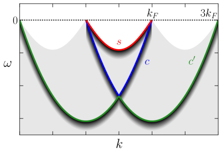
Most of the weight of the one-electron spectral function is generated by transitions to excited states involving creation of one hole in the band, one hole in the band, plus low-energy particle-hole processes in such bands. Processes where both holes are created away from the band and band Fermi points and , respectively, contribute to the spectral-function continuum. Processes where the band hole is created at momentum values spanning its band interval and the hole (spinon) is created near one of its Fermi points contribute to the and branch lines whose spectra run from and , respectively. Since in such processes the band hole is created away from the band Fermi points, we call it a (charge) hole mobile impurity. Finally, processes where the band hole is created at momentum values in the interval and the hole (holon) is created near one of its Fermi points contribute to the branch line whose spectrum runs from . In the case of these processes it is the band hole that is created away from the corresponding band Fermi points. Hence we call it (spin) hole mobile impurity. See a sketch of such spectra in Fig. 1. In the remainder of this paper the charge (and spin) hole mobile impurity is merely called (and ) impurity.
The one-electron operators matrix elements between energy eigenstates in the expressions for the spectral function involve phase shifts and the charge parameter whose value is determined by them. Its range for the present lattice systems is , where the bare parameter defined by Eq. (48) of Appendix A refers to the 1D Hubbard model. Note that the model in Eq. (1), becomes the 1D Hubbard model at the bare charge parameter value, . In this limit, the SDS exponent reads with and for and , respectively. For there is a transformation Ma_17 for each fixed value of and such that and . This maps the 1D Hubbard model onto the model, Eq. (1), upon gently turning on . Consistent with this result, for . For the corresponding SDS exponent intervals are . ¡ The phase shifts in the one-electron matrix elements play a major role in our study by appearing explicitly in the expressions of the momentum-dependent exponents of the one-electron removal spectral function. These phases shifts are and . Specifically, and are the phase shifts, respectively, imposed on a particle of band momentum by a and impurity created at momentum and . (Their explicit expressions are given below.) The charge parameter is given by a superposition of charge-charge phase shifts,
The expressions for the exponents of spectral functions also involve the phase shifts and induced on a particle of band momentum by a and impurity created at momentum and , respectively. Their simple expressions are invariant under the transformation and, due to the spin symmetry, are interaction, density, and momentum independent. (Except for in the expression at .)
For small energy deviations and near the branch lines and branch line, the spectral function behaves as,
| (2) |
respectively. Here and are , , and dependent constants for energy and momentum values corresponding to the small energy deviations and , respectively, and are high energies beyond those of the TLL.
The upper bounds of the constants , , and in Eq. (2) are known from matrix elements and sum rules for spectral weights, but their precise values remain in general an unsolved problem. The expressions for the spectra and exponents are given in Eqs. (33) and (35) of Appendix A, respectively. As discussed in Appendix B, the MQIM-HO also applies to the low-energy TLL limit in which such exponents have different expressions. For the present high-energy regime, they have the same expressions as for the MQIM-LO except that the phase shift in that of the spectral function exponents and has MQIM-HO additional terms.
That the branch line coincides with the edge of the support for the spectral function ensures that near it the line shape is power-law like, as given in Eq. (2). For the branch likes, which run within the spectral weight continuum, the lifetime in Eq. (2) is very large for the interval , so that the expression given in that equation is nearly power-law like, . The finite-range interaction effects increase upon decreasing in the interval where . In it the corresponding impurity relaxation processes associated with large lifetimes and in Eq. (2) for the intervals for which and , respectively, start transforming the power-law singularities into broadened peaks with small widths. Such effects become more pronounced upon further decreasing in the interval . As discussed in more detail below in Sec. V.4, for ranges for which the exponents and become positive upon decreasing , the relaxation processes wash out the peaks entirely.
III The effective-range expansion and the unitary limit
III.1 The effective-range expansion
As we shall establish in detail below, the finite-range electron interactions have their strongest effects in the charge-charge interaction channel. In contrast, for the charge-spin channel, the renormalization factor of the phase shift,
| (3) |
remains that of the MQIM-LO.
For small relative momentum of the impurity of momentum and particle of momentum the phase shift associated with the charge-charge channel obeys an effective range expansion,
| (4) |
This equation is the same as for three-dimensional (3D) s-wave scattering problems if is replaced by Bethe_49 ; Blatt_49 . The first and second terms involve the scattering length and effective range , respectively. The third and higher terms are negligible and involve the shape parameters Bethe_49 ; Blatt_49 ; Burke_11 ; Kermode_90 ; Landau_65 .
One finds that in the bare charge parameter limit, , the effective range expansion reads where , is the bare phase shift defined in Eqs. (43)-(47) of Appendix A, and is the bare scattering length.
Due to the 1D charge-spin separation at all MQIM energy scales, the repulsive electronic potential gives rise to an attractive potential associated with the interaction of the particle and impurity at a distance . To go beyond the MQIM-LO, we must explicitly account for the general properties of whose form is determined by that of . The corresponding relation between the electron and particle representations is discussed see Appendix C. The attractive potential is negative for where is a non-universal distance that either vanishes or is much smaller than the lattice spacing . Moreover, for the present class of systems vanishes for large as,
| (5) |
Here is a non-universal reduced mass, is an integer determined by the large- behavior of , and is a length scale whose dependence for is given below in Sec. IV. (And is twice the van der Waals length at ).
Since has asymptotic behavior , the scattering length, effective range, and shape parameter terms in Eq. (4) only converge if , , and , respectively Burke_11 . We shall find that agreement with the experimental results is achieved provided that the effective range studied in Sec. IV is finite and this requires that in Eq. (5).
Similarly to the potentials considered in Refs. Flambaum_99, and Gribakin_93, , the class of potentials with large-distance behavior, Eq. (5) and whose depth is larger that the scattering energy of the corresponding interactions considered here are such that the positive “momentum” obeys a sum rule of general form,
| (6) |
Here where is a relative fluctuation that involves two uniquely defined yet non-universal scattering lengths, and . As justified in Sec. IV, in the present unitary-limit case discussed in Sec. III.2, they are the bare and renormalized scattering lengths, respectively, defined in that section. The physically important renormalized charge parameter range is for which . The term in Eq. (6) refers to a potential boundary conditionFlambaum_99 ; Gribakin_93 with for that interval. (In that regime, the expressions in Eq. (6) are similar to those in Eqs. (4) and (6) of Ref. Flambaum_99, with , , , and corresponding to , , , and , respectively.) A function for the interval for which merely ensures that the sum rule in Eq. (6) continuously vanishes as .
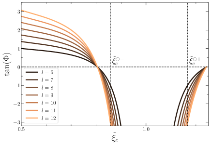
Our choice of potentials with large- behavior given in Eq. (5) is such that the sum rule, Eq. (6), is obeyed yet for small the form of is not universal and is determined by the specific small- form of itself. The zero-energy phase in Eq. (6) whose physics is further clarified below can be expressed as,
| (7) |
Indeed, for and . Here for with the ratio decreasing from at to at . For it is an increasing function of such that for finite.
The universal form of the spectral function near the singularities, Eq. (2), is determined by the large behavior of , Eq. (5), and sum rules, Eqs. (6) and (7). In the spectral-weight continuum, its form is not universal, as it depends on the specific small form of determined by .
The length scale in Eq. (5) is found below in Sec. IV to obey the inequality in units of . ( in such units corresponds to the important parameter of Ref. Flambaum_99, in units of Bohr radius Å with and corresponding to and , respectively.) This inequality justifies why for and implies that in Eq. (7) has for large values. This is consistent with the above mentioned requirement of the scattering energy of the residual interactions of the particles and impurity being smaller than the depth of the potential well, which since must be large. Here is a small non-universal potential-dependent value such that at which and reaches its maximum value.
III.2 The unitary limit and the scattering lengths
As confirmed below in Sec. IV, the expression for the phase shift in the thermodynamic limit,
| (8) |
for remains the same as for the MQIM-LO. Its use along with that of for the bare phase shift in the leading term of the corresponding effective-range expansions gives the scattering lengths. In the thermodynamic limit they read,
| (9) |
respectively. This is known as the unitary limit Zwerger_12 ; Horikoshi_17 .
The validity of the MQIM-HO refers to this limit, which occurs provided that , , and as confirmed below that . The dependence of the bare charge parameter on the density and is defined by Eq. (48) of Appendix A. It is such that for and for for and for and at for both and . This implies that provided that the relative momentum obeys the inequality . This excludes electronic densities very near and for all values and excludes large values for the remaining electronic densities.
The phase shifts incurred by the particles from their interactions with the impurity created at momentum have band momenta in two small intervals and near the band Fermi points and , respectively. As discussed in Appendix B, the creation of an impurity in the band intervals and refers to the low-energy TLL regime. Its velocity becomes that of the low-energy particle-hole excitations near and , respectively. In this regime, the physics is different, as the impurity loses its identity, since it cannot be distinguished from the band holes (TLL holons) in such excitations.
The small momentum can be written as . The unitary limit refers to the corresponding low-density of particle scatterers with phase shift and band momentum values and near and , respectively. They, plus the single impurity constitute the usual dilute quantum liquid of the unitary limit whose density is thus . is such that and for . Here is the number of particle scatterers in .
In the thermodynamic limit one has that is very small or even such that . Consistent with this result, the following relations of the usual unitary limit of the dilute quantum liquid unitary limit Zwerger_12 , and hold. The effective range derived in Sec. IV is such that as . The unitary limit requirement that in the thermodynamic limit is the reason that the value is excluded from the regime in which the MQIM-HO is valid.
Importantly, although both and , the ratio is finite. Since below in Sec. IV we confirm that and are in Eq. (6) the scattering lengths given by Eq. (9), the value of in their ratio expression is found to be controlled by the potential though in the sum rules provided in Eqs. (6) and (7) as,
| (10) |
The first expression on the right-hand side of this equation is specific to the present 1D quantum problem and follows directly from Eq. (9). Hence in the present case in Eq. (6) can be expressed as,
| (11) |
One finds from the use of Eq. (10) that effects of the finite-range interactions controlled by relative fluctuation in , Eq. (6), are stronger for when , , and in Fig. 2. Upon increasing within the intervals and , the relative fluctuation increases from for to for , crossing and at and , respectively. Upon further increasing , the ratio decreases from to at , crossing at . Here and are given by Eqs. (12) and (13) with where is the bare scattering length in Eq. (9). For the electronic density and interaction (the values used in Sec. V for Bi/InSb(001)), , , and .
The renormalized charge parameter intervals for which and for which refer to two qualitatively different problems. Importantly, the value in the transformation is uniquely defined for each of these two intervals solely by the bare charge parameter , Eq. (48) of Appendix A, the integer quantum number in the potential large- expression, Eq. (5), and its sum rule zero-energy phase , Eq. (7), as follows:
| (12) | |||||
where,
| (13) |
IV The effective range
IV.1 The effective-range general problem and cancellation of its unwanted terms
The MQIM-HO accounts for the higher terms in the effective range expansion, Eq. (4), so that as anticipated the phase shift acquires an additional term, , relative to the MQIM-LO,
| (14) |
The second term in the expression for the phase shift reveals that its renormalization is controlled by the scattering lengths associated with the leading term in the effective range expansion. The bare phase shift in that expression is defined in Eqs. (43)-(47) of Appendix A. Furthermore, the function in the expression of vanishes for and is such that its use in the term on the left-hand side of Eq. (4), , gives rise to all the shape parameter terms in the expansion, Eq. (4), beyond the two leading terms, .
Fortunately, in the unitary limit all properties that are characterized by these higher-order terms become irrelevant also for . Hence is given by , which gives at small . (That vanishes in the thermodynamic limit confirms that at the phase shift has the same value , Eq. (8), as for the MQIM-LO.)
Both the unitary limit and the fact that for the scattering energy of the residual interactions of the particles and impurity are much smaller than the depth of the potential will play important roles in the following derivations of the effective range in the expression of , Eq.(14).
First, note that the phase shift term (see Eq. (14)) of in the effective range expansion, Eq. (4), contributes only to the leading term in that expansion , . Thus it does not contribute to the effective range . Indeed, that phase shift term reads , Eq. (8), at whereas it vanishes at , so that in the thermodynamic limit the derivative is ill defined.
For a potential with large- behavior, , Eq. (5), the effective range in the phase shift term of Eq. (14) follows from standard scattering-theory methods, and becomes Joachain_75 ; Preston_75 ; Flambaum_99
| (15) |
This integral converges provided that .
The bare limit boundary condition for all corresponds to the wave function in Eq. (15). It is the zero-energy solution of the Schrödinger equation for the free motion,
Here is the reduced mass of the particle and impurity. The function then has the form for all .
In contrast, the wave function in Eq. (15) is associated with the potential induced by the potential in Eq. (1). The former is associated with the interaction of the particle and impurity. That wave function is thus the solution of a corresponding Schrödinger equation at zero energy,
| (16) |
with the boundary condition . It is normalized at as .
The charge parameter interval for which that corresponds to the second expression in Eq. (12) is of little interest for our studies, as similar values are reachable by the 1D Hubbard model. Two boundary conditions that must be obeyed by in that parameter interval are and . They are satisfied by the following phenomenological effective range expression,
| (17) |
In the case of the interval for which that corresponds to the first expression in Eq. (12), the explicit derivation of the integral in the effective range expression, Eq. (15), simplifies because the inequalities in units of and are found to apply, as reported in Sec. III. This ensures that for the scattering energy of the residual interactions of the particles and impurity is much smaller than the depth of the potential .
The following analysis applies to general scattering lengths , finite or infinite, and potentials with these general properties. They imply that the large- function obeying a Schrödinger equation,
whose attractive potential is given by its large-distance asymptotic behavior , Eq. (5), which has the general form,
| (18) |
This expression can be used for all provided that at small distances where it is deep is replaced by a suitable energy-independent boundary condition. This is also valid for 3D s-wave scattering problems whose potentials have the above general properties and whose scattering lengths are parametrically large Flambaum_99 .
and are in Eq. (18) independent constants and and where and are Bessel functions of argument,
From the use in Eq. (18) of the asymptotic behavior, , of the Bessel functions for and thus one finds that the normalization at as requires that,
| (19) |
and
| (20) |
It is convenient to write the integrand in Eq. (15) as where,
| (21) |
and the functions and are given by,
| (22) |
and
| (23) | |||||
respectively.
The separation in Eq. (21) is convenient because the divergences all appear in the functions and . That and have the expressions given in Eqs. (19) and (20), respectively, ensures that both and read and thus the divergences from and exactly cancel each other under the integration of Eq. (15). Hence can be expressed as,
| (24) |
IV.2 The energy-independent boundary condition
The only role of , Eq. (22), is to cancel within , Eq. (21), under the integration in Eq. (15). In the general expression for the effective range given in that equation, is the solution of Eq. (16) with the actual potential defined in its full domain, . The alternative use of Eq. (24), which was derived by using the function large- expression, Eq. (18), for the whole domain , also leads to the effective range, Eq. (15). This applies provided that is replaced at small distances near , where it is deep, by the energy-independent boundary condition defined below. It accounts for the effects from for small distances.
In the unitary limit the inverse scattering length, , which appears in the expression, Eq. (20), is at the middle of negative and positive values and could refer to or . Hence in that limit there is not much difference between the repulsive and attractive scattering cases. As discussed in Ref. Castin_12, for the case of two particles with a s-wave interaction, the scattering lengths in the attractive and repulsive cases of the unitary limit merely refer to different states of the same scattering problem.
For a potential with a finite scattering length and having the general properties reported above, at small distances where the potential is deep it can be replaced by an energy-independent boundary condition such that the ratio reads where . Here is a potential dependent zero-energy phase, , and for . Moreover, where , is a relative fluctuation, and given in Eq. (20) is a mean scattering length determined by the asymptotic behavior of the potential through the integer and the length scale . For instance, in terms of the constants and , of the scattering problem studied in Ref. Flambaum_99, , the ratio on the left hand side of the above boundary condition reads where .
For the present range the length scale whose expression is given below is finite in the unitary limit and thus the related length scale in Eq. (20) is also finite. It follows both that and the constant , Eq. (20), vanishes. This result is clearly incorrect. The reason is that we have have not yet accounted for the behavior of at small distances through a suitable energy-independent boundary condition. In the case of the unitary limit, this boundary condition renders both and in Eq. (20) finite. Specifically, the scattering length is suitably mapped under it into a finite scattering length , so that is mapped onto the following corresponding finite constant ,
| (25) |
Here yet may be different from in Eq. (10). Indeed, the relation is insensitive to such phase differences. In the unitary limit the boundary condition is thus equivalent to a transformation such that .
The energy-independent boundary condition in Eq. (25) is in terms of the finite scattering length such that is given by , similarly to scattering problems of the same universality class whose scattering lengths are parametrically large Flambaum_99 ; Gribakin_93 . The positivity of often occurs for potentials that for large distances are attractive Flambaum_99 . If were negative, , then would be given by , which would violate both the requirements that and that in the bare limit, .
Importantly, the cancellation is independent of the value of the scattering length in the expressions for and . Hence all results associated with Eqs. (15)-(24) remain the same, with replaced by . This includes the effective range , Eq. (24), remaining determined only by .
The main property of the transformation is the corresponding exact equality of the ratios, . This actually justifies why the scattering lengths and , Eqs. (9), can be used in in Eq. (6). That transformation is also the mechanism through which the renormalized scattering length emerges in .
Hence similarly to finite- scattering problems of the same universality class, as for instance those studied in Refs. Flambaum_99, and Kishi_17, , the relations of general form, Eq. (6), apply. In the present unitary limit the scattering length ratio in them equals the ratio also given by Eq. (10). The sum rule , Eq. (7), encodes the effects from for small distance near , referring to the interval around .
IV.3 The effective range dependence on the scattering length finite ratio
The use of the function , Eq. (23), with the constants and given in Eqs. (19) and (25), respectively, in Eq. (24) leads for to,
After performing the integrations, one finally reaches the following expression valid for the present charge parameter interval and ,
| (26) |
That here the coefficient,
| (27) |
is identified with the lattice spacing results from the imposition of having the same value for and . The coefficients and in Eq. (26) can be expressed in terms the usual function and are given by,
| (28) |
respectively. They decrease from at to and for .
The effective range , Eq. (26), appears in the expression of the spectral function exponents and , Eq. (35) of Appendix A, through the expression for the phase shift , Eq. (14). for is excluded, as it is outside the range of validity of the unitary limit. The values found below in Sec. V for Bi/InSb(001) are given in Table 5. They obey the unitary limit inequality, .
The effective range, Eq. (26), can alternatively be expressed in terms of the ratio involving the finite scattering lengths and defined by Eqs. (20) and (25), respectively.
The expression for the lattice spacing , Eq. (27), contains important physical information: Its inverse gives the following expression valid for for the length scale in the potential expression, Eq. (5), and the related length scale , Eq. (7),
| (29) |
Here is given by at , reaches a maximum at , and decreases to as , so that in units of as given in Table 5. Thus for .
As in the case of 3D s-wave atomic scattering problems Flambaum_99 ; Gribakin_93 , this shows that for the scattering energy of the interactions of the particles and impurity is indeed much smaller than the depth of the potential well. This confirms the consistency of the derivation of the effective range for that assumed the validity of such properties.
The length scales involved in the MQIM-HO description are explicitly defined in Table 2.
| Length scale | Description |
|---|---|
| length scale in the large- potential decay with exponent , , Eqs. (5) and (29) | |
| lattice spacing related to (twice the van der Waals length at ) as given in Eq. (27) | |
| and | scattering lengths at and , respectively, within the transformation, Eqs. (9) and (10) |
| effective range for the interval of physical interest, Eqs. (26) and (28) |
V ARPES in Bi/InSb(001)
V.1 Brief information on the sample preparation and ARPES experiments
Concerning the preparation of the Bi/InSb(001) surface, a substrate InSb(001) was cleaned by repeated cycles of Ar sputtering and annealing up to K. Bi was evaporated on it up to nominally monolayers (ML): One ML is defined as the atom density of bulk-truncated substrate. Then, the substrate was flash-annealed up to K for seconds. The resulting surface showed a () low-energy electron diffraction pattern.
Although the Bi/InSb(001) surface state is formed by evaporating Bi on the InSb substrate, in addition to Bi also In and Sb are found at the surface, modified from their bulk positions by Bi evaporation. Hence Bi, In, and Sb can all be significant sources of the surface electronic states. Detailed information of the characterization of the Bi/InSb(001) surface sample is provided in Ref. Ohtsubo_15, .
ARPES measurements were performed at eV and taken at K in the CASSIOPÉE beamline of SOLEIL synchrotron. The photoelectron kinetic energy at and the overall energy resolution of the ARPES setup were calibrated by the Fermi edge of the photoelectron spectra from Mo foils attached to the sample. The energy resolution was 20 meV. The ARPES taken at K is shown in Fig. 3.
The theoretical predictions reported in this paper refer to (i) the -plane location of the high-energy Bi/InSb(001) MDC and EDC ARPES peaks and (ii) the value of the power-law SDS exponent associated with the angle integration to detect the low-energy suppression of the photoelectron intensity that were performed at , near the boundary of the () surface Brillouin zone ().
V.2 Criteria for agreement between ARPES and the present theory
Refs. Ohtsubo_15, and Ohtsubo_17, found strong experimental evidence that Bi/InSb(001) at momentum component and temperature K displays 1D physics with an SDS exponent that for small eV has values in the interval .
As discussed and justified below in Sec. VI.1, the one-electron spectral properties of Bi/InSb(001) are expected to be controlled mainly by the interplay of one dimensionality and finite-range electron interactions, despite a likely small level of disorder. Consistent with an SDS exponent larger than stemming from finite-range interactions Schulz_90 , here we use the MQIM-HO to predict one-electron spectral properties of Bi/InSb(001).
As discussed in Sec. VI.1, Bi/InSb(001) is a complex system and some of its experimental properties beyond those studied here may involve microscopic processes other than those described by the MQIM-HO and the Hamiltonian, Eq. (1). This includes coupling to two-dimensional (2D) physics if is smoothly changed to .
As reported in Sec. III.1, the MQIM-HO can describe both the low-energy TLL regime and the spectral function, Eq. (2), at high energies near the -plane singularities. At and in the vicinity of those singularities, the renormalization from its bare form is determined by the large behavior of , Eq. (5), and its sum rules, Eqs. (6) and (7), which refer to a high energy regime that goes well beyond the TLL limit.
Hence we can predict two properties of the one-electron spectral function : (i) the location in the plane of the experimentally observed high-energy peaks in the ARPES MDC and EDC and (ii) the value of the low-energy SDS exponent . Our theoretical results describe the former high-energy experimental data taken at K for which the smearing of the spectral function singularities by thermal fluctuations is negligible. The quantitative agreement with the corresponding experimental data taken at fixed momentum reached below provides further evidence of 1D physics and electron finite-range interactions in Bi/InSb(001).
| Agreement | Description |
|---|---|
| First type | overall -plane shapes of the theoretical branch-line spectra, Eq. (33), versus ARPES experimental spectra |
| Second type | -plane location of the singularities corresponding to negative exponents, Eq. (35), versus ARPES peaks |
| Third type | SDS exponent from the dependence of the exponents, Eq. (35), on versus its low- experimental value |
A first type of agreement of the theoretical branch-line energy spectra with the -plane shape of the ARPES image spectra must be reached for well-defined fixed values of electronic density and interaction . Through Eq. (48) of Appendix (A), these uniquely determine the value of the bare charge parameter to be used in the transformations suited to Bi/InSb(001). In addition, that first type of agreement also determines the value of the transfer integral .
The experimental values of the lattice spacing and of the momentum width of the spectra at provide the Fermi momentum and thus the electronic density . At the density , the ratio of the experimental energy bandwidths of the branch line spectrum and of the and branch line spectra at momentum uniquely determine . (See such energy bandwidths in the sketch of the theoretical spin and charge and branch lines in Fig. 1.) Finally, the experimental values of and determine the value of the transfer integral .
As discussed below in Sec. V.3, from the available experimental data it is not possible to trace the energy dispersion of the branch line. However, combining the experimental data on the EDC with kinematic constraints of the MDC provides information about the most probable value of the energy at which its bottom is located, which equals the branch line energy bandwidth .
A second type of agreement is between the momentum interval and corresponding energy interval for which the exponents , , and , Eq. (35) of Appendix A, are negative and the -plane location of the experimentally observed high-energy ARPES MDC and EDC peaks. That agreement must be reached at the fixed and values and corresponding bare charge parameter value obtained from the first type of agreement. This second type of agreement is reached at some values of the integer quantum number in the large- potential expression, Eq. (5), and of the renormalized charge parameter (and thus of , see Eqs. (12) and (13)).
For the theoretically predicted high-energy ARPES peaks located on the branch line, there is only limited experimental information. Hence we start by finding the and values at which the second type of agreement is reached concerning the momentum intervals where the exponents and are negative and the corresponding -plane location of the experimentally observed high-energy ARPES MDC and EDC peaks. Fortunately, it turns out that the values lead to a prediction of location in the -plane of the high-energy ARPES peaks associated with the branch line that is consistent with the available experimental EDC data.
This second type of agreement is reached for specific values. This then provides a prediction for the SDS exponent obtained from a different low-energy experiment that detects the suppression of the photoelectron intensity. That the SDS exponent determined by the values for which the second type of agreement is reached is also that measured within the low-energy angle integrated photoemission intensity then becomes the required third type of agreement.
In the Lehmann representation of the spectral function, the first and second types of agreement correspond to the energy spectra and the overlaps of the one-electron matrix elements, respectively. The exponents in Eq. (35) of Appendix A involved in the second type of agreement depend both on and momentum-dependent phase shifts and . There is no apparent direct relation between the high-energy ARPES MDC peaks and the low-energy SDS. That the MQIM-HO describes the main microscopic mechanisms behind the specific one-electron spectral properties of Bi/InSb(001) then requires that the third type of agreement is fulfilled.
The three types of agreement between theory and experiment are explicitly described in Table 3.
V.3 Searching for agreement between theory and experiments
V.3.1 First type of agreement
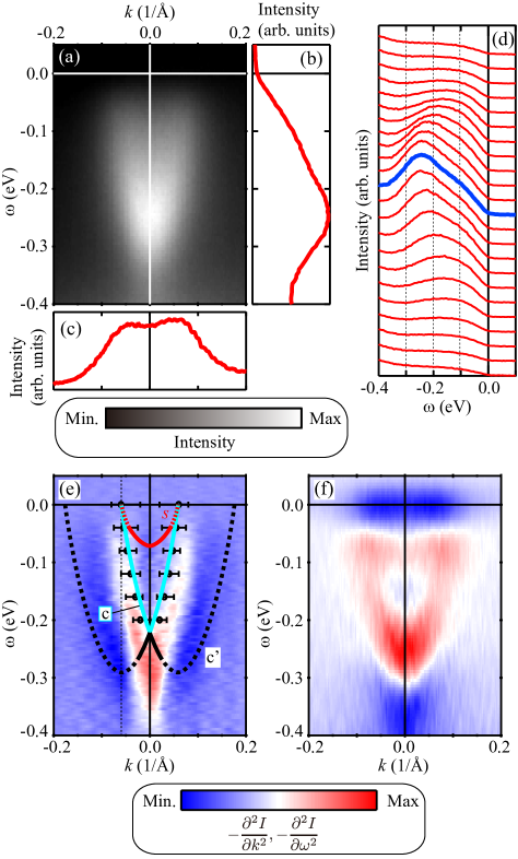
The MDC spectral shape plotted in Fig. 3(c) displays two peaks centered at well defined Fermi momentum values and , respectively. Furthermore, the experimental circles (with error bars) in Fig. 3(e) clearly indicate that the MDC peaks are located on two lines that in the limit of zero energy start at such two Fermi momenta. Since the experimental data lead to , one finds from a small electronic density, .
The experimental value of the branch line energy bandwidth is directly extracted from analysis of the experimental MDC data provided in Fig. 3(e). From analysis of the EDCs in Fig. 3(d) alone one finds that there is a uncertainty eV concerning the energy at which the bottom of the branch line is located. It is clear that in this energy region there is a hump that cannot be explained by assuming the single peak at eV, which refers to the bottom of the branch line.
The zero-energy level of the theoretically predicted downward-convex parabolic-like dispersion of the branch line plotted in Fig. 3(e) (see also sketch depicted in Fig. 1) refers to the Fermi level. Hence the branch line energy bandwidth equals that of its bottom. While the energy range uncertainty of that bottom energy is experimentally rather wide, one can lessen it by combining the experimental ARPES MDC intensity distribution shown in Fig. 3(c) with its kinematical constraints, which follow from the finite-energy bandwidth of the theoretical branch line. One then finds that the most probable value of the branch line bottom energy and thus of is between and eV.
The maximum momentum width of the ARPES MDC intensity distribution shown in Fig. 3(c) for energy eV allowed by such kinematic constraints involves the superposition of two maximum momentum widths , centered at and , respectively. Within the MQIM-HO, these kinematical constraints explain the lack of spectral weight in well-defined -plane regions shown in Fig. 1. Fortunately, the lines that limit such regions without spectral weight only involve the band dispersion spectrum.
In the case of the spectral weight centered at and , respectively, such kinematical constraints imply that for each energy value the corresponding maximum momentum width reads,
| (30) |
where and the band dispersion spectrum is given in Eq. (33) of Appendix A.
For the kinematical constraints, Eq. (30), are those of a TLL, , consistent with Orgad_01 . However, for energy larger than the branch line energy bandwidth , which is that at which the branch line bottom is located in the experimental data, there are no kinematical constraints.
The absolute value of the derivative with respect to of the ARPES MDC intensity plotted in Fig. 3(c) increases in a interval and decreases for . Theoretically, the ARPES MDC intensity should be symmetrical around . Its actual experimental shape then introduces a small uncertainty in the value of . The relatively large intensity in the tails located at the momentum region is explained by the larger uncertainty in the branch line bottom energy . Indeed, the ARPES MDC under consideration refers to an energy eV within that uncertainty. And, as given in Eq. (30), there are no kinematic constraints for .
One can then identify the most probable value of within its uncertainty interval as that for which at the energy eV the kinematic constraints would limit the ARPES MDC intensity to momentum values within the interval . The corresponding momenta are the inflection points at which the derivative of the variation of the ARPES MDC intensity with respect to changes sign in Fig. 3(c). The momentum width associated with is thus that of the ARPES MDC shown in that figure if one excludes the tails.
The corresponding maximum momentum width , Eq. (30), of the two overlapping spectral weights centered at and , respectively, that at eV would lead to the kinematic constraint , so that . According to the kinematic constraints in Eq. (30), this is fulfilled when at so that the branch line energy spectrum reads eV. Accounting for the combined and uncertainties, the most probable value of the energy bandwidth is larger than eV and smaller than eV, as that of the theoretical branch line plotted in Fig. 3(e).
At electronic density the best second type of agreement between theory and experiments discussed in the following is reached within that combined uncertainty by the and values that are associated with the energy bandwidth of such a theoretical branch line. They read and eV, as determined from the corresponding ratio and experimental value in Fig. 3(e). Hence within the MQIM-HO the first type of agreement with the ARPES spectra is reached by choosing these parameter values for the electronic density .
V.3.2 Second type of agreement
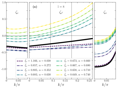
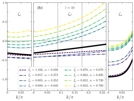
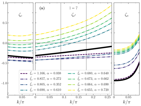
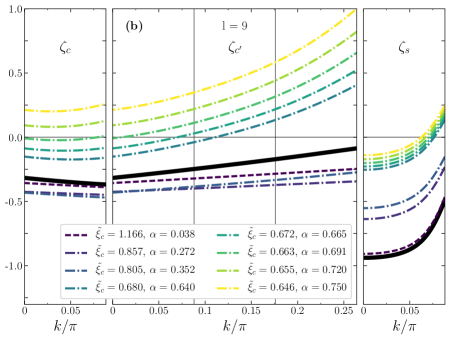
The second type of agreement involves the theoretical exponents , Eq. (35) of Appendix A. They are plotted for and as a function of the momentum in Fig. 4(a) for and in Fig. 4(b) for . In Appendix A, they are plotted as a function of for several additional values of .
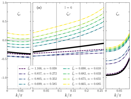

The different curves in each figure are associated with different values of the charge parameter and thus of the SDS exponent and effective range . The black solid lines refer to the bare charge parameter limit, . The values , , and correspond to , , and , respectively.
As justified in Sec. V.2, we start by finding the and values at which the second type of agreement is reached. It refers to the momentum intervals (and corresponding energy ranges) at which the exponents and are negative. Those are required to agree with the corresponding -plane location of the experimentally observed high-energy ARPES MDC and EDC peaks in Figs. 3(e) and (f), respectively. This reveals that the integers and the values of the charge parameter and corresponding SDS exponent for which agreement is reached are those for which the exponents and , Eq. (35) of Appendix A, in the spectral-function expression near the and branch lines, Eq. (2), are negative for and , respectively.
In the case of the exponent , the momentum appearing in the interval is such that is vanishing or very small in the thermodynamic limit. It is the experimental value of the small theoretical band momentum associated with the low density of particle scatterers near the band Fermi points and considered in Sec. III.2.
Concerning the momentum interval for which the exponent must be negative, there is a small uncertainty in the value of . It is such that where in Fig. 3(e) is the momentum width of the ARPES image crossed by the branch line.
This small uncertainty, which in the units used in the figures corresponds to , implies corresponding small uncertainties in the and values at which for each agreement with the experimentally observed high-energy ARPES MDC and EDC peaks is reached. The corresponding two limiting values of such and uncertainties at which the exponent in Fig. 4 and in Figs. 5 and 6 of Appendix A crosses zero at and , respectively, are given in Table 4 for each integer .
Following the direct relation between the and branch lines spectra, that ensures that the exponent is indeed negative for intervals where , as also required for the second type of agreement to be reached.
Hence regarding the and branch lines, agreement between theory and experiments is reached by the and values that in Fig. 4 and in Figs. 5 and 6 of Appendix A correspond to the branch line exponent curves crossing zero between and . (In such figures only the two corresponding branch line exponent curves crossing zero at and , respectively, are plotted.)
| () | () | () | () | |
|---|---|---|---|---|
The theoretical branch line exponent , Eq. (35) of Appendix A, does not depend on the integer quantum number . For the values for which the branch line exponent curves cross zero between and in Fig. 4 and in Figs. 5 and 6 of Appendix A, the exponent is negative in corresponding intervals and thus positive for . Here is a function of , , and and are the two momentum values at which vanishes.
The predicted location at of the ARPES MDC peaks associated with the branch line cannot be confirmed from the available experimental data. Indeed and as mentioned in Sec. V.2, it is not possible to extract from such data the dispersion of that line. However, the corresponding energy intervals are consistent with the available experimental data from the EDCs in Fig. 3(d). Here is the bottom of the branch line energy, as estimated in Sec. V.3.1 from the interplay of the kinematical constraints, Eq. (30), and the ARPES MDC shown in Fig. 3(c) for eV.
V.3.3 Third type of agreement
From the above results we see that for agreement with the experimentally observed high-energy ARPES MDC and EDC peaks in Figs. 3(e) and (f) is reached by the exponents curves referring to and values belonging to the small intervals reported in Table 5. The overlap of the subintervals obtained for each given in that table then leads to the theoretical predictions and .
Table 5 also provides the corresponding intervals of the effective range in units of the lattice spacing that refer to first and second types of agreements. The effective range dependence on the bare charge parameter , renormalized charge parameter , and integer quantum number values at which such agreements have been reached is defined by combining Eqs. (10) and (26). That table also provides the values of the length scale in the same units whose dependence on is given in Eq. (29). Upon increasing from to , the effective range values for which there is agreement with the experiments change from to , respectively.
According to the analysis of Sec. V.3.2, agreement with the experimentally observed high-energy -plane ARPES MDC and EDC peaks distribution has been reached for the SDS exponent range . The third type of agreement between theory and experiments defined in Sec. V.3.2 is reached provided that such a predicted SDS exponent range agrees with the values measured within the low-energy angle integrated photoemission intensity. An experimental uncertainty of the SDS exponent was found for 0.1 eV in Ref. Ohtsubo_15, .
The remarkable quantitative agreement of the MQIM-HO predictions within the third criterion reported in Sec. V.3.2 provides evidence of finite-range interactions playing an active role in the Bi/InSb(001) spectral properties and confirms the 1D character of its metallic states also found in Ref. Ohtsubo_15, .
| 6.3 | |||||
| 6.5 | |||||
| 6.5 | |||||
V.4 Interplay of relaxation processes with the momentum dependence of the exponents
Here we discuss the physical mechanisms within the MQIM-HO that underlie the dependence of the exponents , , and on the charge parameter . These exponents are plotted in Fig. 4 and in Figs. 5 and 6 of Appendix A.
In the bare charge parameter limit, , the exponents being negative or positive just refers to a different type of power-law behavior near the corresponding charge and spin branch lines. For , this applies only to the spin branch line. It coincides with the edge of support of the one-electron removal spectral function that separates -plane regions without and with finite spectral weight. Hence conservation laws impose that, near that line, the spectral function remains of power-law form, Eq. (2), for both intervals and . As confirmed from an analysis of the branch-line exponents plotted in Fig. 4 and in Figs. 5 and 6 of Appendix A, the effect of decreasing the charge parameter from its initial bare value (and thus increasing the SDS exponent from ) is merely to increase the spin branch line exponent . Except for two regions near and corresponding to , that exponent remains negative, so that the singularities prevail. In the complementarily small momentum regions near defined by where the exponent is positive, the line shape remains of power-law type.
Analysis of the and branch-line exponents curves plotted in the same figures reveals that the situation is different for the one-electron removal spectral function in the vicinity of the charge and branch lines, Eq. (2). These are located in the continuum of the one-electron spectral function. The physics is though different for the subintervals and , respectively.
Smoothly decreasing from its initial bare value to , produces effects quite similar to those of increasing within the 1D Hubbard model to Carmelo_18 . Indeed, these changes render and more negative and lead to an increase of the width of the intervals in which they are negative. Within the interval, a large number of conservation laws that are behind the factorization of the scattering matrix into two-particle scattering processes survive, which tend to prevent the impurity from undergoing relaxation processes. Hence the lifetimes and in Eq. (2) are very large for the intervals for which the corresponding branch line exponents are negative, so that the expression given in the equation for the spectral function near the branch lines is nearly power-law like, .
The effects of the finite-range interactions increase upon decreasing within the interval where for and . Indeed, smoothly decreasing within that interval tends to remove an increasing number of conservation laws, which strengthens the effects of the impurity relaxation processes. Such effects become more pronounced when and , upon further decreasing within the interval .
In the intervals for which the branch line exponents remain negative, the lifetimes in Eq. (2) remain large and the impurity relaxation processes only slightly broaden the spectral-function power-law singularities, as given in Eq. (2). For the complementary ranges for which such exponents become positive upon decreasing and thus increasing , the high-energy singularities are rather washed out by the relaxation processes.
As confirmed by analysis of the curves plotted in Fig. 4 and in Figs. 5 and 6 of Appendix A, starting at and downwards, smoothly decreasing from first gradually enhances the domains where is positive. Further decreasing after the branch line singularities are fully washed out leads to the emergence of a branch line domain starting at and upwards in which that line singularities are finally fully washed out up to below a smaller value.
VI Discussion and concluding remarks
VI.1 Discussion of other effects and properties outside the range of the MQIM-HO
As reported in Sec. V.1, the ARPES data were taken at K and the angle integrations to detect the suppression of the photoelectron intensity were performed at , near the boundary of the () surface Brillouin zone ().
As shown in Fig. 2(b) of Ref. Ohtsubo_15, , at there is an energy gap between the spectral features studied in this paper within a 1D theoretical framework and a bulk valence band. Due to that energy gap, the coupling between the two problems is negligible, which justifies that the system studied here corresponds to 1D physics.
Smoothly changing from to corresponds to smoothly turning on the coupling to the 2D physics. As shown in Fig. 2(a) of Ref. Ohtsubo_15, , at the energy gap between the spectral features studied in this paper and that bulk valence band has been closed. The study of the microscopic mechanisms involved in the physics associated with turning on the coupling to the 2D physics by smoothly changing from to is an interesting problem that deserves further investigation.
Another interesting open problem refers to theoretical prediction of the MDC for extended momentum intervals and of the EDC for corresponding energy ranges. The universal form of the spectral function near the singularities, Eq. (2), is determined by the large behavior of the potential , Eq. (5), which follows from that of the potential in Eq. (1), and potential sum rules, Eqs. (6) and (7). As reported in Eqs. (12) and (13), the value of the renormalized charge parameter behind the renormalization of the phase shifts in the exponents of that spectral function expression, Eq. (2), is indeed controlled by the value of the initial bare charge parameter , the integer quantum number associated with the potential large- behavior, Eq. (5), and the zero-energy phase determined by that potential sum rules, Eqs. (6) and (7). Plotting a MDC for extended momentum intervals and an EDC for corresponding energy ranges is a problem that involves non-universal properties of the one-electron removal spectral function. This would require additional information of that function in -plane regions where it is determined by the detailed non-universal dependence on of the specific electronic potential suitable to Bi/InSb(001).
Another interesting issue refers to the validity of the MQIM-HO to describe the Bi/InSb(001) one-electron spectral properties. The question is whether the interplay of one dimensionality and electron finite-range interactions is indeed the main microscopic mechanism behind such properties. As in all lattice electronic condensed matter systems, it is to be expected that there are both some degree of disorder effects and electron-electron effects in the Bi/InSb(001) physics. However, we can provide evidence that the interplay of latter effects with the Bi/InSb(001) metallic states one dimensionality is the dominant contribution to the one-electron removal spectral properties.
The first strong evidence that this is so is the experimentally observed universal power-law scaling of the spectral intensity . (Here refers to the Fermi-level energy.) For instance, at and finite and at and low it was found in Ref. Ohtsubo_15, to have the following TLL behaviors for Bi/InSb(001),
| (31) |
respectively, where is the SDS exponent.
If there were important effects from disorder, its interplay with electron-electron interactions would rather give rise in the case of 1D and quasi-1D systems to a spectral intensity with the following behaviors Rollbuhler_01 ; Mishchenko_01 ; Bartoscha _02 ,
| (32) |
for . Here is the bare diffusion coefficient and is a constant that depends on the effective electron-electron interaction and electronic density.
The behaviors in Eq. (32) are qualitatively different from those reported in Eq. (31), which are those experimentally observed in Bi/InSb(001). This holds specially for , in which case disorder effects cannot generate such a temperature power-law scaling. Also the experimentally found behavior disagrees with that implied by Eq. (32).
Further, in the limit of low and , the MQIM-HO describes the corresponding TLL limit in which the universal power-law scaling of the spectral intensity has the behaviors reported in Eq. (31). Theoretically, the value of the SDS exponent depends on those of the electronic density , the interaction , and the renormalized charge parameter . Within the MQIM-HO phase shifts constraints, its values span the intervals .
The theoretically predicted value has been determined from agreement of the one-electron spectral function, Eq. (2), with the ARPES peaks location in the -plane. The quantitative agreement then reached refers to the experimental value obtained for at eV in Ref. Ohtsubo_15, . For low temperatures and the MQIM-HO also leads to the behavior given in Eq. (31).
Finally, despite bismuth Bi, indium In, and antimony Sb being heavy elements, the present 1D surface metallic states do not show any detectable spin-orbit coupling effects and nor any related Rashba-split bands. In this regard, it is very important to distinguish the system studied in this paper with 1-2 monatomic layers of Bi thickness whose ARPES data were first reported in Ref. Ohtsubo_15, from the system with a similar chemical name which was studied in Ref. Kishi_17, , which refers to 5-20 monatomic layers of Bi thickness. One expects, and indeed observes, significant qualitative differences in these two systems.
VI.2 Concluding remarks
In this paper we have discussed an extension of the MQIM-LO used in the theoretical studies of the ARPES in the line defects of MoSe2 Ma_17 . This MQIM-type approach Imambekov_09 ; Imambekov_12 accounts only for the renormalization of the leading term in the effective range expansion of the charge-charge phase shift, Eq. (4). As shown in Ref. Cadez_19, , this is a good approximation if the effective range of the interactions of the particles and the impurity is of about one lattice spacing.
The MQIM-HO developed in this paper accounts for the renormalization of the higher terms in the effective range expansion of the charge-charge phase shift, Eq. (4). It applies to a class of 1D lattice electronic systems described by the Hamiltonian, Eq. (1), which has longer range interactions. The quantum problem described by that Hamiltonian is very involved in terms of many-electron interactions. However, we found that a key simplification is the unitary limit associated with the scattering of the fractionalized charged particles by the impurity. We have shown a theory based on the MQIM-HO with finite-range interactions, Eq. (1), applies to the study of some of the one-electron spectral properties of Bi/InSb(001) measured at momentum component and temperature K.
Consistent with the relation of the electron and particle representations discussed in Appendix C, the form of the attractive potential associated with the interaction of the particles and the impurity at a distance is determined by that of the electronic potential in Eq. (1). The universal behavior of the spectral function near the singularities given in Eq. (2) whose -plane location refers to that of the experimentally observed high-energy ARPES peaks, is determined by the large behavior of shown in Eq. (5) and sum rules, Eqs. (6) and (7). Otherwise the spectral function expression in the continuum is not universal.
Despite the limited available experimental information about the ARPES peaks located on the spin branch line, we have shown that all the three criteria associated with the different types of agreement between theory and experiments considered in Sec. V.2 are satisfied. This provides further evidence to that given in Ref. Ohtsubo_15, for the interplay of one dimensionality and finite-range interactions playing an important role in the one-electron spectral properties of the metallic states in Bi/InSb(001).
Acknowledgements.
J. M. P. C. acknowledges the late Adilet Imambekov for discussions that were helpful in producing the theoretical part of the paper. Y. O. and S.-i. K. thank illuminating discussions to obtain and analyze the ARPES dataset by Patrick Le Fèvre, François Bertran, and Amina Taleb-Ibrahimi. J. M. P. C. would like to thank Boston University’s Condensed Matter Theory Visitors Program for support and the hospitality of MIT. J. M. P. C. and T. Č. acknowledge the support from Fundação para a Ciência e Tecnologia (FCT) through the Grants UID/FIS/04650/2013, PTDC/FIS-MAC/29291/2017, and SFRH/BSAB/142925/2018, NSAF U1530401 and computational resources from Computational Science Research Center (CSRC) (Beijing), and the National Science Foundation of China (NSFC) Grant 11650110443.Appendix A Useful quantities
The spectra of the branch lines in the expressions for the one-electron removal spectral function in Eq. (2) have for the MQIM-HO the same general form as for the MQIM-LOMa_17 ; Cadez_19 and read,
| (33) |
Here and are the and particle energy dispersions, respectively. For the and band momentum intervals at which the and impurities, respectively, are created under one-electron excitations the energy dispersions and corresponding group velocities read,
| (34) |
Here the bare energy dispersions and are defined below and where is given in Eq. (54) of Appendix C. It reads for whereas for the range of most interest for our studies where . For the latter range, its limiting behaviors are
The renormalization in Eq. (34) is related to the expression , Eq. (54) of Appendix C, and the corresponding ratio of the renormalized and bare band Fermi velocities Carmelo_TT . That the spin dispersion remains invariant under finite-range interactions whereas the charge dispersion bandwidth and the charge Fermi velocity are slightly increased as the range of interactions increases is known from numerical studies Hohenadler_12 . (See the related charge and spin spectra in Fig. 7 of Ref. Hohenadler_12, and the corresponding discussion.)
In the MQIM-HO, the momentum dependent exponents in the expressions for the one-electron removal spectral function, Eq. (2), also have the same form as for the MQIM-LO. However, some of the quantities in their following expressions have additional MQIM-HO terms,
| (35) |
These exponents are plotted in Figs. 4(a) and 4(b) as a function of the momentum within the MQIM-HO for , , and even values and , respectively. In this appendix they are plotted in Figs. 5 and 6 for even values and odd values , respectively.
The phase shifts and that in Eq. (35) appear in units of are defined in Eqs. (3) and (14), respectively. The bare phase shifts and in the latter equations are defined below. The MQIM-HO phase shift term in Eq. (14) accounts for effects of finite-range interactions beyond the MQIM-LO through the spectral function exponents and in Eq. (35).
The small momentum in Eq. (35) such that is in general smaller than the momentum considered in the discussions of Sec. V.3.2. It has the same role for the band as for the band, concerning the crossover between the low-energy TLL and high-energy regimes. As discussed below in Appendix B, for physical momenta associated with creation of the impurity at in the small band momentum in the absolute value interval and creation of the impurity at in the small band momentum absolute value interval corresponding to the low-energy TLL regime the expressions for the exponents, Eq. (35), are not valid.
The bare energy dispersions and in Eq. (34) are defined as follows,
| (36) |
The distributions and appearing here are solutions of the coupled integral equations,
| (37) |
and
| (38) | |||||
The rapidity distribution functions and for the and impurity occupancies and , respectively, in the arguments of the auxiliary dispersions and in Eq. (36) are defined in terms of their inverse functions where and where , respectively. The latter are defined by the equations,
| (39) | |||||
The parameter in Eqs. (36), (38), and (39) is defined by the relations,
| (40) |
Furthermore, the distributions and in Eq. (39) are the solutions of the coupled integral equations,
| (41) |
and
| (42) | |||||
In the and limits the solution and the use of Eqs. (36)-(42) leads to the following analytical expressions for the dispersions and ,
and
respectively.

The bare phase shifts and in the expressions of the phase shifts and provided in Eqs. (3) and (14), respectively, are given by,
| (43) |
where the quantities and where are particular cases of the rapidity dependent auxiliary phase shifts and . Those are the solution of the following integral equations,
| (44) |
and
| (45) |
respectively, where,
| (46) | |||||
| (47) | |||||
and is the usual function.
In the and limits the solution and the use of Eqs. (43)-(47) leads to the following analytical expressions for the bare phase shifts and ,
and
respectively
The dependence on the electronic density and interaction of the bare charge parameter is defined by the following relation and equation,
| (48) |
where is given in Eq. (47). Its limiting behaviors are,
where for .
Finally, the extended domain of relative fluctuation , Eq. (11), is briefly discussed. For the physical processes of interest for the problem studied in this paper, in Eq. (48) varies in the domain . The relative fluctuation in Eq. (11) where applies though to all finite negative values of and . This refers to an extended domain .
Its new subinterval corresponds to electronic potentials of the same general form, and for , as those in Eq. (1) but for which . In the general case there are transformations within which the function is smoothly turned on from at to (i) positive and (ii) negative values, respectively. Considering all such processes and values leads to charge parameters that vary in the intervals and , respectively, for which the relations given in Eqs. (12) and (13) remain valid. The scattering length symmetry relations, and , then confirm that both and in .
Within the new subinterval the SDS exponent varies in the physically irrelevant range . refers here to . Only transformations for which both and refer to processes contributing to the physical problem studied in this paper.
Appendix B Relation to the TLL regime and crossover to it
Both the MQIM-LO and the MQIM-HO also apply to the low-energy TLL regime whose spectral-function exponents near the branch lines are different from those given in Eq. (35). In the high energy regime whose spectral function expression, Eq. (2), was used in this paper to predict the -plane location of the high-energy Bi/InSb(001) ARPES peaks, the velocity of the or impurity is different from the velocity at the or band Fermi points, respectively.
In contrast, in the TLL regime the (i) or (ii) impurity is created in its band at a momentum in one of the intervals (i) and or (ii) and . (Here both and .) The group velocity of that impurity thus becomes that of the low-energy particle-hole excitations near the corresponding Fermi point (i) and or (ii) and , respectively. Hence they loses their identity, as they cannot be distinguished from the or holes (usual holons and spinons) in such excitations.
The exponents in Eq. (35) can be rewritten as, . Here and for the one-electron removal branch line and and for both the one-electron removal and branch lines, which correspond to different intervals of the band momentum in .
It turns out that in the TLL regime the expressions for the exponents in the above equation lose one of the four s. It is the whose sign of is that of the Fermi point whose velocity is the same as the or impurity velocity. The expressions of the exponents, Eq. (35), in the high-energy spectral function expressions Eq. (2) used in the theoretical study of the Bi/InSb(001) high-energy ARPES peaks are thus different from those of the TLL regime.
In the case of a large finite system, there is a cross-over regime between the high energy regime and the low-energy TLL regime within which the above quantity or is gradually removed as the energy decreases. This cross-over regime refers to -plane regions whose momentum and energy widths are very small or vanish in the thermodynamic limit. It is an interesting theoretical problem, but the details of its physics have no impact on the specific problems discussed in this paper.
Appendix C Electron and particle representations
In the bare limit, , the particles are directly related to rotated electrons for which double occupancy is a good quantum number for . Their operators,
| (49) |
and are generated from those of the electrons by the unitary operator . It is uniquely defined in Ref. Carmelo_17, in terms of the matrix elements between all the model energy eigenstates.
The present quantum problem is defined in a subspace without rotated-electron double occupancy. Hence merely removes the corresponding electron double occupancy from all sites around that of index at which or acts. In that subspace, the electron double occupancy reads where for and , , and . Here is the particle creation operator and and are usual spin operators written in terms of rotated-electron operators.
The same rotated-electron basis and corresponding particle representation can be used for the renormalized Hamiltonian, Eq. (1). The difference relative to the bare limit is that the states generated from the fractionalized particles configurations are not in general energy eigenstates but in the relevant subspaces for which the impurity has a large lifetime, they have overlap with single energy eigenstates.
The operator preserves the distance between electrons, being the same for rotated electrons. The rotated-electron anti-commutation relations that follow from unitarity imply that the particle operators obey a fermionic algebra, and . In the rotated-electron basis the Hamiltonian, Eq. (1), has an infinite number of terms given by the Baker-Campbell-Hausdorff formula,
| (50) |
Here , has the same expression in terms of rotated-electron operators as in terms of electron operators, and all higher terms have a kinetic nature. Indeed, the expression of only involves the three kinetic operators , , and in where gives the change in the number of rotated-electron doubly occupied sites, and,
| (51) | |||||
Consistent with the finite-range electron interactions having their strongest effects in the charge-charge interaction channel, in Eq. (50) can be expressed solely in terms of the charge particle operators as,
| (52) | |||||
Here for whole Hilbert space where the rotated-electron operators are related to those of the electrons in Eq. (49).
Importantly, despite the infinite number of terms in the Hamiltonian, Eq. (1), when expressed in terms of the rotated-electron operators, Eq. (50), its relevant term for our study is that in Eq. (52) with replaced by rotated-electron potential renormalized by the higher kinetic terms in the expansion, Eq. (50). The latter are in turn renormalized by . only involves the operators and the four operators , , and ,
| (53) | |||||
Higher kinetic terms also only involve the operators and , Eq. (51), and at different relative sites.
The interaction between a particle at site and the impurity at site refers to a Hamiltoninan term of the form . In terms of , it refers to suitably transformed operators and corresponds to Carmelo_TT . The part of the renormalization by the infinite kinetic energy terms beyond in Eq. (50) that contributes to the universal properties is accounted for by the transformation. The non-universal part is within the non-universal inverse reduced mass to which is also proportional, .
The Fourier transform of controls the band energy dispersion and velocity renormalization. At it has the universal behavior Carmelo_TT ,
| (54) | |||||
Here is the bare band velocity at defined by Eq. (34) of Appendix A for , , and is related to the enhancement parameter in that equation as and thus determines its value, . The expression in Eq. (54) gives at and and for , as required by the properties of the related potential for .
On the other hand, the Fourier transform of the potential is found in Ref. Carmelo_TT, to read at where the coefficient is given by for and for . The quantity is related to the phase-shift and matrix-element renormalization.
References
- (1) C. Blumenstein, J. Schäfer, S. Mietke, S. Meyer, A. Dollinger, M. Lochner, X. Y. Cui, L. Patthey, R. Matzdorf, and R. Claessen, Nature Phys. 7, 776 (2011).
- (2) J. Voit, Rep. Prog. Phys. 58, 977 (1995).
- (3) S. Tomonaga, Prog. Theor. Phys. 5, 544 (1950).
- (4) J. M. Luttinger, J. Math. Phys. 4, 1154 (1963).
- (5) J. M. P. Carmelo, K. Penc, and D. Bozi, Nucl. Phys. B 725, 421 (2005); 737, 351 (E) (2006).
- (6) A. Imambekov and L. I. Glazman, Science 323, 228 (2009).
- (7) A. Imambekov, T. L. Schmidt, and L. I. Glazman, Rev. Mod. Phys. 84, 1253 (2012).
- (8) H. J. Schulz, Phys. Rev. Lett. 64, 2831 (1990).
- (9) H. Bethe, Z. Phys. 71, 205 (1931).
- (10) E. H. Lieb and F. Y. Wu, Phys. Rev. Lett. 20, 1445 (1968).
- (11) M. J. Martins and P. B. Ramos, Nucl. Phys. B 522, 413 (1998).
- (12) J. M. P. Carmelo and P. D. Sacramento, Phys. Reports 749, 1 (2018).
- (13) R. Claessen, M. Sing, U. Schwingenschlögl, P. Blaha, M. Dressel, and C. S. Jacobsen, Phys. Rev. Lett. 88, 096402 (2002).
- (14) B. J. Kim, H. Koh, E. Rothenberg, S.-J. Oh, H. Eisaki, N. Motoyama, S. Uchida, T. Tohyama, S. Maekawa, Z.-H. Shen, and C. Kim, Nature Phys. 2, 397 (2006).
- (15) K. Schönhammer and M. Meden, J. of Elec. Spect. and Rel. Phenom. 62, 225 (1993).
- (16) Y. Ma, H. C. Diaz, J. Avila, C. Chen, V. Kalappattil, R. Das, M.-H. Phan, T. Čadež, J. M. P. Carmelo, M. C. Asensio, and M. Batzill, Nature Comm. 8, 14 231 (2017).
- (17) Y. Ohtsubo, J.-I. Kishib, K. Hagiwara, P. Le Fèvre, F. Bertran, A. Taleb-Ibrahimi, H. Yamane, D.-I. Ideta, M. Matsunami, K. Tanaka, and S.-i. Kimura, Phys. Rev. Lett. 115, 256404 (2015).
- (18) Y. Ohtsubo, J.-I. Kishib, K. Hagiwara, P. Le Fèvre, F. Bertran, A. Taleb-Ibrahimi, and S.-i. Kimura, J. Elec. Spectr. Rel. Phenom. 220, 37 (2017).
- (19) H. A. Bethe, Phys. Rev. 76, 38 (1949).
- (20) J. M. Blatt and J. D. Jackson, Phys. Rev. 76, 18 (1949).
- (21) C. J. Joachain, Quantum Collision Theory (North-Holland, Amsterdam, 1975).
- (22) Preston, M. A., and R. K. Bhaduri, ,+ Structure of the Nucleus (Addison-Wesley, Reading, Ma, 1975).
- (23) V. V. Flambaum, G. F. Gribakin, and C. Harabati, Phys. Rev. A 59, 1998 (1999).
- (24) T. Čadež, L. Li, E. V. Castro, and J. M. P. Carmelo, Phys. Rev. B 99, 155109 (2019).
- (25) L. D. Landau and E. M. Lifshitz, Quantum Mechanics: Non-Relativistic Theory (Pergamon, Oxford, 1965).
- (26) M. W. Kermode and W. van Dijk, Phys. Rev. C 42, 1891 (1990).
- (27) P. G. Burke, R-Matrix Theory of Atomic Collisions (Springer-Verlag, Heidelberg, 2011), Sec. 1.4.
- (28) R. G. Newton, Scattering Theory of Waves and Particles (Springer-Verlag, Berlin, 1982).
- (29) W. Zwerger (Editor), The BCS-BEC Crossover and the Unitary Fermi Gas, Lecture Notes in Physics Vol. 836, (Springer-Verlag, Heidelberg, 2012).
- (30) M. Horikoshi, M. Koashi, H. Tajima, Y. Ohashi, and M. Kuwata-Gonokami, Phys. Rev. X 7, 041004 (2017).
- (31) D. J. Dean and M. Hjorth-Jenson, Rev. Mod. Phys. 75, 607 (2003).
- (32) G. F. Gribakin and V. V. Flambaum, Phys. Rev. A 48, 546 (1993).
- (33) D. Orgad, S. A. Kivelson, E. W. Carlson, V. J. Emery, X. J. Zhou, and Z. X. Shen, Phys. Rev. Lett. 86, 4362 (2001).
- (34) J. Rollbühler and H. Grabert, Phys. Rev. Lett. 87, 126804 (2001).
- (35) E. G. Mishchenko, A.V. Andreev, and L. I. Glazman, Phys. Rev. Lett. 87, 246801 (2001).
- (36) L. Bartoscha and P. Kopietz, Eur. Phys. J. B 28, 29 (2002)
- (37) J. Kishi, Y. Ohtsubo, T. Nakamura, K. Yaji, A. Harasawa, F. Komori, S. Shin, J. E. Rault, P. Le Fèvre, F. Bertran, A. Taleb-Ibrahimi, M. Nurmamat, H. Yamane, S. Ideta, K. Tanaka, and S. Kimura, Phys. Rev. Materials 1, 064602 (2017).
- (38) J. M. P. Carmelo, T Čadež, D. K. Campbell, M. Sing, and R. Claessen, (unpublished).
- (39) M. Hohenadler, S. Wessel, M. Daghofer, and F. F. Assaad, Phys. Rev. B 85, 195115 (2012).
- (40) J. M. P. Carmelo and T Čadež, Nucl. Phys. B 914, 461 (2017).
- (41) Y. Castin and F. Werner, Lecture Notes in Phys. 836, 127 (2012).