Improving Accuracy of Electrochemical Capacitance and
Solvation Energetics in First-Principles Calculations

Abstract

Reliable first-principles calculations of electrochemical processes require accurate prediction of the interfacial capacitance, a challenge for current computationally-efficient continuum solvation methodologies. We develop a model for the double layer of a metallic electrode that reproduces the features of the experimental capacitance of Ag(100) in a non-adsorbing, aqueous electrolyte, including a broad hump in the capacitance near the Potential of Zero Charge (PZC), and a dip in the capacitance under conditions of low ionic strength. Using this model, we identify the necessary characteristics of a solvation model suitable for first-principles electrochemistry of metal surfaces in non-adsorbing, aqueous electrolytes: dielectric and ionic nonlinearity, and a dielectric-only region at the interface. The dielectric nonlinearity, caused by the saturation of dipole rotational response in water, creates the capacitance hump, while ionic nonlinearity, caused by the compactness of the diffuse layer, generates the capacitance dip seen at low ionic strength. We show that none of the previously developed solvation models simultaneously meet all these criteria. We design the Nonlinear Electrochemical Soft-Sphere solvation model (NESS) which both captures the capacitance features observed experimentally, and serves as a general-purpose continuum solvation model.

I Introduction

The electrochemical double layer plays a central role in the chemistry of a wide variety of processes including electrocatalysis, biocatalysis, and corrosion. Over the last century, the fundamental structure and properties of the electrochemical double layer have been characterized extensively, facilitated by advances in spectroscopy Fried and Boxer (2015); Fleischmann et al. (1973), microscopy Wiechers et al. (1988) and single-crystal electrochemistryClavilier (1980). The charge and electric field distributions in the double layer vary with applied potential in complex ways, exhibiting a rich interplay between the surface structure, electrolyte and adsorbates.Baskin and Prendergast (2017) Measuring, understanding, and quantitatively modeling these distributions is vital because they can strongly affect chemical reactions at the electrochemical interface.

The charge and electric field distributions collectively contribute to the overall change in charge with potential, or electrochemical capacitance of the double layer. This capacitance frequently contains signatures of ion adsorption and chemical reactions at the interface. Fundamental studies of the intrinsic response of the double layer therefore employ single-crystalline metal surfaces and a non-adsorbing electrolyte. Fig. 1 shows the experimental capacitance curves of Ag(100) in aqueous KPF₆ electrolyte,Valette (1982) the archetypal capacitance of a metal surface in non-adsorbing aqueous electrolyte. These curves exhibit a characteristic wide ‘hump’ shape that is nearly independent of electrolyte concentration, and a narrower ‘dip’ at the potential of zero charge (PZC) that becomes increasingly pronounced at low electrolyte concentrations.Hamelin (1986); Parsons (1990); Trasatti (1979); Damaskin and Frumkin (1974)

The concentration-dependent dip in the electrochemical capacitance can be explained by the Gouy-Chapman-Stern (GCS) modelStern (1924), one of the simplest models for the interface. This model contains two capacitance contributions in series: a concentration-independent contribution from the dielectric region devoid of ions next to the electrode (Helmholtz capacitance), and the strongly concentration and potential-dependent contribution from ions that are further away (diffuse capacitance). The latter ionic contribution is strongly nonlinear with the potential and grows exponentially as the potential deviates from the neutral value, producing the dip feature in the net series capacitance. However, this model does not exhibit the reduction in capacitance further away from the potential of zero charge (the hump).

More generally, the total series capacitance observed experimentally can be decomposed into a diffuse contribution, and a concentration-independent but potential-dependent contribution containing the hump.Grahame (1947); Parsons and Zobel (1965) Theories to explain this hump have historically included dielectric saturation of water, adsorption of ions, and ion packing.Trasatti (1979); Damaskin and Frumkin (1974); Schmickler and Henderson (1986); Saradha and Sangaranarayanan (1998); Amokrane and Badiali (1992); Markovich et al. (2014)

Capturing complex capacitance behavior in calculations that include electronic structure effects of the surface and the reaction species is essential for understanding double layer effects on adsorbates and chemical reactions.Xiao et al. (2016); Jason D. Goodpaster and Head-Gordon (2016); Garza et al. (2018) However, accurately capturing capacitance features with strictly ab initio methods would require ab initio molecular dynamics (AIMD) calculations that are unfeasibly large because of the large number of solvent molecules and electrolyte ions necessary for meaningful statistics, and the long equilibration time of the electrolyte distribution. A tractable alternative is to couple density-functional theory (DFT) calculations of the electronic-structure sensitive reactants and surface with a continuum representation of the electrolyte. A continuum solvation model suitable for this purpose must then capture the effect of non-adsorbing electrolytes, while the electrode and specific adsorbates are included explicitly in the DFT calculation.

In this paper, we demonstrate the shortcomings of current state-of-the-art solvation models for metallic electrodes in non-adsorbing, aqueous electrolyte, and find that they do not reproduce the capacitance features that are experimentally observed. We then use a simple extension of the Gouy-Chapman-Stern model to illustrate the need for a dielectric-only region at the interface, and nonlinear dielectric effects in the bulk electrolyte. We formulate the Nonlinear Electrochemical Soft-Sphere (NESS) solvation model, an extension of the recently-developed Soft-Sphere (atomic-sphere-based) solvation modelFisicaro et al. (2017), that includes the necessary nonlinear effects and dielectric-only region. We show that NESS, used in conjunction with DFT calculations of the metal surface, can capture the magnitude, shape, and ionic concentration dependence of the measured electrochemical capacitance of Ag(100) immersed in aqueous KPF₆, while simultaneously remaining accurate for solvation energies of ions and neutral molecules.

II Current solvation models

Continuum solvation models approximate the effect of a liquid environment by placing the solute (treated quantum-mechanically using DFT) in a cavity within a dielectric continuum. Ions in an electrolyte additionally contribute a Debye screening response in the continuum. Beyond this ansatz, solvation models differ in the construction and parametrization of the cavity, as well as the treatment of the continuum dielectric and ionic response. Broadly, determining the cavity from the solute electron density (iso-density) and/or electrostatic potential involves a few easily-determined parameters, whereas determining the cavity using atom-centered spheres involves many parameters and more complexity but offers greater flexibility. Additionally, the approximations used to model the dielectric and ionic continuum regions can be either linear or nonlinear in response to the applied potential. Nonlinearity of the dielectric response arises from saturation of solvent dipoles aligning to the local electric field, while nonlinearity of the ionic response arises from the Boltzmann occupation factor of the ions at the local potential. The latter exponential increase in local ion concentration results in increased localization of ions near the electrode and increased diffuse contribution to the capacitance, giving rise to the capacitance dip as discussed for GCS theory above. Finally, the ionic and dielectric cavities can be separated by a distance typically denoted by $x_{2}$ in GCS theory, or they can share the same cavity ($x_{2}$=0).

Model	Response		Cavities
	$\epsilon$	$\kappa$	Type	$x_{2}\neq 0$
LinearPCMGunceler et al. (2013); Letchworth-Weaver and Arias (2012) =VASPsolMathew et al. (2014)	L	L	$n$	No
CANDLESundararaman and Goddard (2015)	L	L	$n,\phi$	No
SCCSAndreussi et al. (2012); Dupont et al. (2013)	L	L	$n$	No
Anderson and JinnouchiJinnouchi and Anderson (2008)	L	NL	$n$	Yes
Dabo et al. 2010Dabo et al. (2010)	L	NL	$n$	Yes
NonlinearPCMGunceler et al. (2013); Sundararaman and Schwarz (2017)	NL	NL	$n$	No
Soft-sphereFisicaro et al. (2017)	L	none	Atom	No
NESS [this work]	NL	NL	Atom	Yes

Table 1: Categorization of solvation models for electrochemistry by linearity of fluid dielectric ($\epsilon$) and ionic ($\kappa$) response, cavity parametrization type, and presence of a separate ionic cavity ($x_{2}\neq 0$). Here L = linear, NL = nonlinear, $n$ = solute electron density (iso-density models), $\phi$ = solute electrostatic potential and Atom = atomic spheres.

Table 1 summarizes the above choices for the predominant solvation models used for electrochemistry, most of which adopt linear dielectric and ionic responses, precluding treatment of the capacitance dip and hump, as we show below. Additionally, simultaneous accuracy for properties of molecules, ions and surfaces is challenging in iso-density models, because of different ideal cavity sizes for capturing solvation energies of positive and negative solute charges,Sundararaman and Goddard (2015) and for capturing capacitance of metallic surfaces.Sundararaman and Schwarz (2017) The recent Soft-Sphere solvation modelFisicaro et al. (2017) brings the added flexibility of atomic parametrization, traditionally employed only in finite molecular calculations,Tomasi et al. (2005); Marenich et al. (2009) to calculations for periodic systems including solid-liquid interfaces. This model has so far not included ionic response or nonlinearity, and has not yet been applied to electrochemical systems. We take advantage of the flexibility of the atomic parametrization of the Soft-Sphere model, and add the key ingredients required for accurate electrochemical predictions that we show below: a separate ionic cavity ($x_{2}\neq 0$) and nonlinear responses of the dielectric and ions, resulting in the NESS model.

We start by comparing the electrochemical capacitance of Ag(100) in non-adsorbing KPF₆ electrolyte against the capacitance predicted by previously-developed solvation models.Valette (1982) For each solvation model, we perform a series of grand-canonical DFT calculationsSundararaman et al. (2017a) in the JDFTx plane-wave DFT softwareSundararaman et al. (2017b) for 25 uniformly spaced potentials in a range extending 0.8 V on either side of the neutral potential (PZC), and calculate the differential capacitance as a finite-difference derivative. We use a seven-layer Ag(100) slab with $12\times 12\times 1$ $k$-point sampling, cold smearing with width $\sigma=0.01~{}E_{h}$ (see SI for convergence checks), the ‘PBE’ exchange-correlation functional,Perdew et al. (1996) and ‘GBRV’ ultrasoft pseudopotentialsGarrity et al. (2014) with a 20 $E_{h}$ (Hartree) plane-wave cutoff. We set the vacuum/electrolyte spacing to at least three times the Debye screening length for each ionic concentration, additionally employing truncated Coulomb interactionsSundararaman and Arias (2013) to isolate periodic images along the third direction.Dabo et al. (2010)

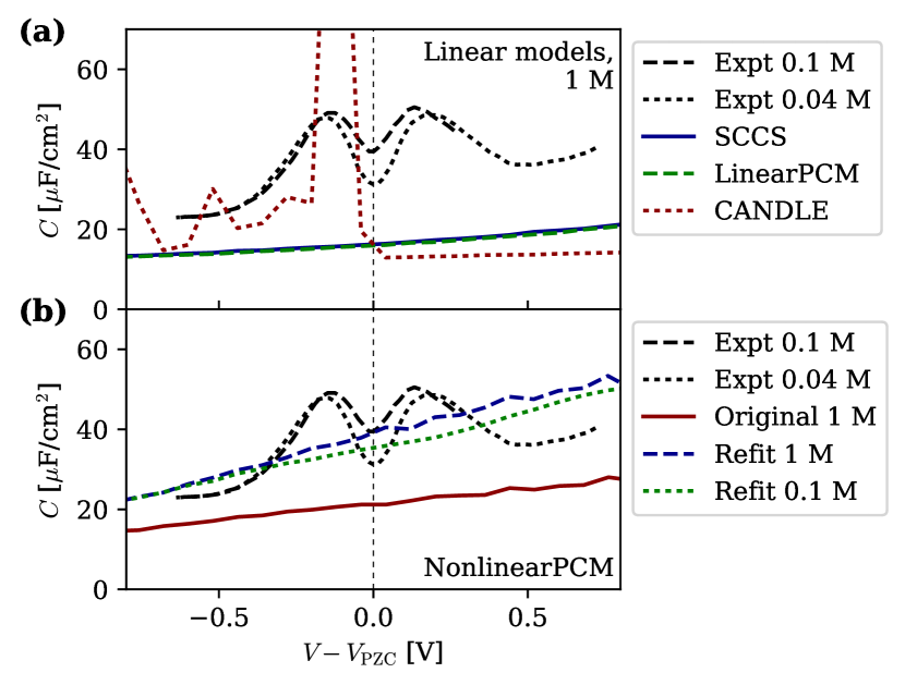
Figure 1: Comparison of capacitance of Ag(100) in KPF₆ with experimental measurementsValette (1982) for (a) linear solvation models including SCCSAndreussi et al. (2012), LinearPCMGunceler et al. (2013) and CANDLESundararaman and Goddard (2015) at a fixed ionic concentration of 1 M (M = mol/L), and (b) nonlinear solvation models including the original parametrization of NonlinearPCMGunceler et al. (2013) and its refit version.Sundararaman and Schwarz (2017) The linear models show none of the potential or concentration dependence features of the experimental data,Sundararaman and Schwarz (2017) while refit NonlinearPCM exhibits only a modest capacitance reduction near the PZC at low ionic concentration.

First, Fig. 1(a) compares the experimental capacitance of Ag(100) with solvation models that solve the linearized Poisson-Boltzmann equation. Of these, the SCCSAndreussi et al. (2012) and LinearPCMGunceler et al. (2013) models lead to a capacitance well below the experimental values, with a slight linear increase with potential, capturing none of the potential or electrolyte-concentration dependence, as expected and discussed previously.Sundararaman and Schwarz (2017) (Note that the commonly used VASPsol modelMathew et al. (2014) re-implements and hence produces identical results to LinearPCM.Gunceler et al. (2013)) The CANDLE Sundararaman and Goddard (2015) model exhibits higher capacitance for negative potentials, along with an unphysical spike when transitioning from positive to negative potentials, because it adjusts the cavity size based on solute electric field to account for asymmetry in solvation of cations and anions. (See SI for a more detailed discussion on the capacitance of CANDLE.)

Next, Fig. 1(b) shows the effect of including dielectric saturation from the rotational response of water molecules as well as the response of electrolyte ions based on the nonlinear Poisson-Boltzmann equation, as in the NonlinearPCM model.Gunceler et al. (2013) The overall capacitance of this model is too low because of a large cavity that results in too low a Helmholtz capacitance, which also dominates the series capacitance and masks nonlinear effects in the diffuse capacitance. Refitting this model’s cavity to match the typical magnitude of the experimental capacitanceSundararaman and Schwarz (2017) exhibits some reduction in capacitance near the PZC for lower ionic concentrations. However, the capacitance still varies almost linearly with potential, with a larger positive slope. This asymmetry with respect to the potential of zero charge results from the electron-density parametrization of the solvent cavity: at positive potentials, the positively charged surface has a lower electron density tail extending from the surface, which pulls the cavity closer and increases the capacitance. Letchworth-Weaver and Arias (2012) This is a particularly large effect for the refit version of NonlinearPCM, because the cavity is determined by a higher electron density threshold, which occurs relatively closer to the metal atoms.

III Toy model

To understand the limitations of existing DFT-based solvation approaches and identify the key pieces necessary to correctly capture electrochemical capacitance, we next study a model system illustrated in Fig. 2(a) that minimally extends GCS theory. The model is composed of a continuum plane of charge representing the metal, a continuum solvent, and a continuum electrolyte. The metal and solvent are separated by a small gap of width $x_{1}$, and the ions are excluded from a solvent region of width $x_{2}$. Assuming the metal is at potential $\phi_{0}$ and extends until $x=0$, the potential $\phi(x)$ for $x>0$ satisfies the nonlinear Poisson-Boltzmann equation

$$\nabla\cdot\epsilon(x,|\nabla\phi|)\nabla\phi +\kappa^{2}(x,\phi)\phi=0,$$ (1)

$$\textrm{with }\epsilon(x,E)\equiv \ 1+\Theta(x-x_{1})(\epsilon(E)-1),$$ (2)

$$\kappa^{2}(x,\phi)\equiv \ \Theta(x-x_{1}-x_{2})\frac{8\pi N_{\mathrm{ion}}e^{2}\sinh\frac{\phi}{k_{B}T}}{\phi}$$ (3)

and with boundary conditions $\phi(0)=\phi_{0}$ and $\phi(\infty)=0$. Here, $\epsilon(E)$ is the field-dependent dielectric constant of liquid water, $N_{\mathrm{ion}}$ is the concentration of a 1:1 electrolyte, $\kappa$ is the inverse Debye screening length, $T$ is temperature, $e$ is the elementary charge, $k_{B}$ is the Boltzmann constant, and $\Theta(x)$ is the Heaviside step function. We use the implicit form $\epsilon(E)=\epsilon_{b}/(1+4(D/D_{0})^{2}+3(D/D_{0})^{4})$ with $D\equiv\epsilon(E)E$, bulk dielectric constant $\epsilon_{b}=78.4$ and fit parameter $D_{0}=36~{}\mu$C/cm², which accurately reproduces SPC/E molecular dynamics predictions for $\epsilon(E)$.Sundararaman et al. (2014) We solve differential equation (1) using a 1D finite-element method for a series of $\phi_{0}$, calculate the metal surface charge density $\sigma=-4\pi\left.\frac{\partial\phi}{\partial x}\right|_{x=0}$ for each, and extract the differential capacitance $\partial\sigma/\partial\phi_{0}$ from a finite difference derivative. In order to consider if ion packing is responsible for the hump, we also solve the modified Poisson-Boltzmann (mPB) equation,Markovich et al. (2014) where the effective $\kappa^{2}$ is instead given by

$$\kappa^{2}(x,\phi)\equiv\Theta(x-x_{1}-x_{2})\frac{8\pi N_{\mathrm{ion}}e^{2}\sinh\frac{\phi}{k_{B}T}}{\phi\left(1+4\eta\sinh^{2}\frac{\phi}{2k_{B}T}\right)}.$$ (4)

For the ion packing fraction $\eta\equiv\frac{4\pi}{3}(R_{\mathrm{cat}}^{3}+R_{\mathrm{an}}^{3})N_{\mathrm{ion}}$, we use an upper-bound cation radius of $R_{\mathrm{cat}}=2.79$ Å  for K⁺ including its hydration shellMarcus (1988), and an anion radius of $R_{\mathrm{an}}=2.41$ Å  for the PF${}^{-}_{6}$ ion.Roobottom et al. (1999)

Fig. 2(b) shows the capacitance predicted by this toy model for the case of the linear dielectric, $\epsilon(0)$. With $x_{1}=0$, the model reduces to GCS theory and the predicted capacitance is much higher than experiment for a typical value of $x_{2}=2.6$ Å. A small vacuum region, $x_{1}=0.1$ Å , is necessary to make the magnitude of the capacitance reasonable; note that this small vacuum gap has the same capacitance as a solvent gap $x_{2}=7.8$ Å  due to the bulk dielectric constant of water, $\epsilon_{b}=78.4$. With a linear dielectric, GCS theory and this new model both produce a constant capacitance far from PZC. Fig. 2(c,d) demonstrate that introducing $\epsilon(E)$, the nonlinear dielectric which includes dielectric saturation, produces the hump feature (the reduction of capacitance far from PZC). Also note that the shape of the hump agrees best with experimental measurements for a theory which includes a solvent-only region, characterized by non-zero $x_{2}=2.6$ Å  in Fig. 2(d). When $x_{2}=0$, as in Fig. 2(c), the width and the height of the capacitance hump are both too large compared to the experiment. Fig. 2(c,d) also show the effects of ion packing, as described by mPB theory with a modified $\kappa^{2}$ as discussed above. Inclusion of ion packing produces a hump-like feature, but with a substantially smaller magnitude than observed in experiment. While this effect may be dominant for ionic liquids Markovich et al. (2014), dielectric saturation is the more important effect for non-adsorbing aqueous electrolyte because of water’s high dielectric constant, the small size of the ions, and the fact that water molecules (rather than ions) are closest to the surface. Additionally, the NonlinearPCM solvation model Gunceler et al. (2013) already includes ion packing effects at a level comparable to mPB theory Markovich et al. (2014) and yet it did not produce an observable hump in Fig. 1.

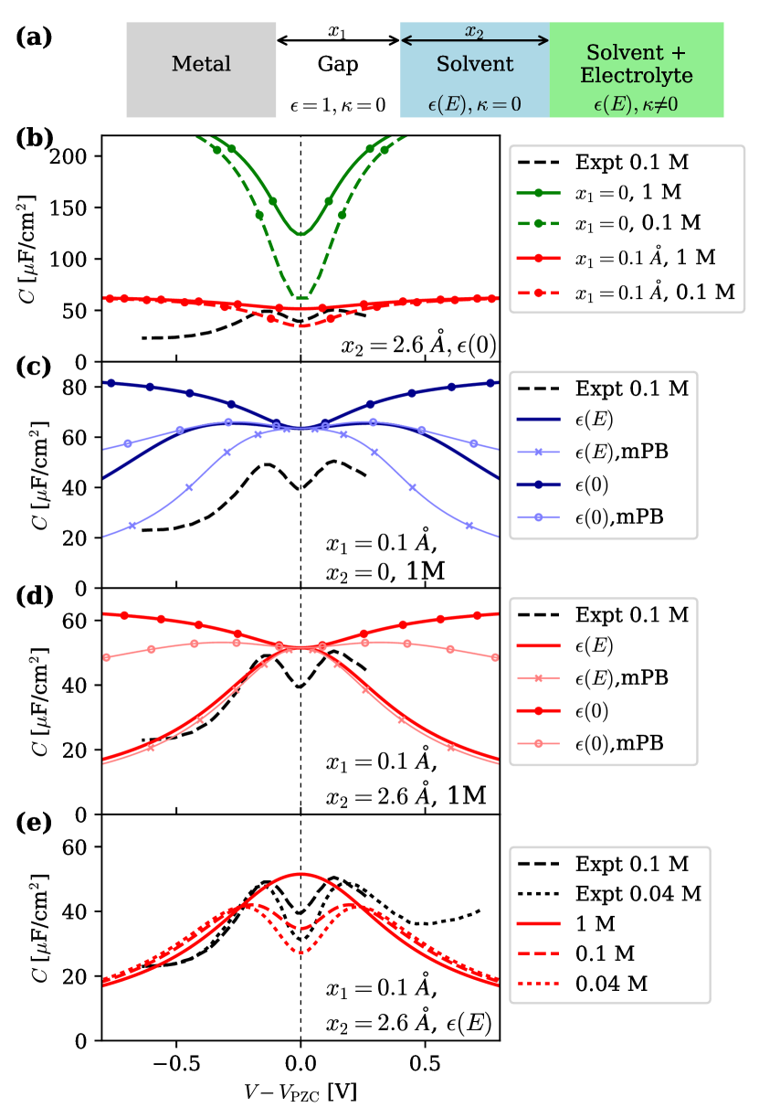
Figure 2: Experimental capacitance of Ag(100)Valette (1982) compared against the toy model illustrated in (a) containing vacuum and solvent gaps of width $x_{1}$ and $x_{2}$ respectively between the metal electrode and electrolyte. (b) Effect of $x_{1}$ on model capacitance for a linear dielectric $\epsilon(0)$, where $x_{1}=0$ is GCS theory. (c,d) Effect of nonlinearity ($\epsilon(E)$) and ion packing as described by the modified Poisson-Boltzmann (mPB) theory on model capacitance for (c) $x_{2}=0$ and (d) $x_{2}=2.6$ Å ; both nonzero solvent gap and dielectric saturation are needed to match experimental shape and mPB theory does not produce a hump to the extent observed in experiment. (e) Electrolyte concentration dependence of the capacitance: nonlinear toy model with $x_{1}$ and $x_{2}$ reproduces hump and dip features well.

Fig. 2(e) shows that the nonlinear toy model with non-zero $x_{1}$ and $x_{2}$ has both the expected capacitance maximum and dips depending on the ionic concentration. However, relatively minor disagreements remain with the experimental curve, including the missing plateaus and slight asymmetry far from PZC, speculated to arise from specific adsorption of water or ions Trasatti (1983); Valette (1981); Damaskin and Frumkin (1974). Understanding the origin of these secondary features seen experimentally and capturing them in a solvation model will be the subject of future work. For instance, future studies could consider the interplay between dielectric saturation and electrolyte packing using a method such as classical density-functional theory with molecular orientations for the solvent Sundararaman and Arias (2014); Sundararaman et al. (2014).

IV New solvation model

Here, we focus on obtaining a continuum solvation model for DFT that captures the hump and dip features qualitatively, and Fig. 2 indicates that such a solvation model must be nonlinear in both the dielectric and ionic responses, and it must have a solvent region that excludes ions ($x_{2}\neq 0$). (Continuum solvation models already include $x_{1}\neq 0$ due to the gap between the electron density of the solute and the solvent cavity.) Table 1 illustrates that none of the previously developed solvation models simultaneously include both nonlinearities and $x_{2}\neq 0$. Additionally, our previous work Sundararaman and Goddard (2015); Sundararaman and Schwarz (2017) found that electron density-based parametrization of solvation model cavities results in limited simultaneous accuracy for properties of molecules, ions, and metal surfaces.

We therefore construct a solvation model with cavities based on atom-centered spheres that is also suitable for calculations of extended systems in the plane-wave basis, starting from the recently proposed Soft-Sphere solvation model.Fisicaro et al. (2017) In this model, the cavity shape function is determined as

$$s(\vec{r})=\prod_{i}\frac{1}{2}\mathrm{erfc}\frac{R_{i}-|\vec{r}-\vec{r}_{i}|}{\sigma}$$ (5)

which goes smoothly from zero in the vicinity of atoms located at positions $\vec{r}_{i}$ to one in the solvent region more than the radius $R_{i}$ away, with a transition width $\sigma$ set to 0.5 Bohr. The sphere radii $R_{i}=fR_{i}^{0}$, where $f$ is a scale parameter fit to solvation energies, and $R_{i}^{0}$ are a set of standard atomic radii, chosen to be the universal force field (UFF) Rappe et al. (1992) van der Waals radii in Ref. 21.

The Soft-Sphere solvation model includes only linear dielectric response and neglects Debye screening from the electrolyte and hence cannot correctly capture electrochemical capacitance. Therefore, we construct the Nonlinear Electrochemical Soft-Sphere (NESS) solvation model by using the Soft-Sphere cavity definition in NonlinearPCM Gunceler et al. (2013), and including an additional ionic cavity so that $x_{2}$ is non-zero. Specifically we set the spatial modulation $s(\vec{r})$ of the nonlinear dielectric response in NonlinearPCM, exactly as given by (5), (instead of a threshold $n_{c}$ on the electron density $n(\vec{r})$ as in Ref. 22). Further, we set the spatial modulation of the nonlinear ionic response to a separate cavity function $s_{\mathrm{ion}}(\vec{r})$, which is still given by (5) except with modified radii $R_{i}^{\mathrm{ion}}=fR_{i}^{0}+x_{2}$, which introduces an electrolyte-excluded solvent region of width $x_{2}$. All remaining details of the model are identical to NonlinearPCM and share most of its implementation in JDFTx,Sundararaman et al. (2017b) including the nonlinear response functions, the term with effective surface tension $t$ to capture non-electrostatic free energy contributions and the algorithms to converge the solvation free energy and to handle charged solutes in periodic boundary conditions. (See Refs. 22 and 33 for further details.)

Model	MAE [kcal/mol]
	Neutral	Cations	Anions	All
Linear dielectric
LinearPCMGunceler et al. (2013)=VASPsolMathew et al. (2014)	1.27	2.10	15.1	3.59
SCCSAndreussi et al. (2012)	1.20	2.55	17.4	3.97
CANDLESundararaman and Goddard (2015)	1.27	2.62	3.46	1.81
Soft-sphereFisicaro et al. (2017)	1.25	6.02	10.4	3.41
Nonlinear dielectric
Orig. NonlinearPCMGunceler et al. (2013)	1.28	16.1	27.0	7.55
Refit NonlinearPCMSundararaman and Schwarz (2017)	1.44	14.4	27.6	7.51
NESS [this work]	1.29	3.67	9.58	2.96

Table 2: Comparison of mean absolute errors (MAEs) in aqueous solvation energies of the same set of 240 neutral molecules, 51 cations and 55 anions between several prominent grid / plane-wave based solvation models. CANDLE yields the lowest MAE in a single parametrization due to charge-asymmetry correction, but that leads to unphysical features in the capacitance (Fig. 1). The NESS model parametrized to neutral solvation energies is reasonably accurate for solvation energies (highlighted below), while simultaneously predicting electrochemical capacitance in good agreement with experiment (Fig. 3). (See SI for additional comparison of ionic parametrizations of the SCCS, Soft-sphere and NESS models.)

We perform solvation free energy calculations of a large set of neutral solutes, cations and anions, including ionic screening (1 M electrolyte) for the ion calculations. We fit the empirical parameters $f$ (cavity scale factor) and $t$ (effective tension = $\alpha+\gamma$ in Ref. 21’s notation) to the solvation free energies. When fit to neutral solutes, we find optimum parameters $f=1.00$ and $t=1.02\times 10^{-5}$, which we use for subsequent calculations here. Table 2 compares the accuracy of this parametrization for solvation energies of neutral solutes, cations and anions with that of several previous solvation models. (See SI for further details on the parametrization, including fits to cation or anion solvation energies alone.) Our new NESS model performs comparably to the linear Soft-Sphere model, and in its parametrization to neutral solutes, is substantially more accurate than the original NonlinearPCM.Gunceler et al. (2013) It still falls short of CANDLE,Sundararaman and Goddard (2015) which is able to deliver the best overall accuracy for solvation free energies within a single parametrization because it accounts for charge asymmetry. However, that feature of CANDLE results in unphysical capacitance predictions, as shown in Fig. 1 and discussed above and in the SI.

Using the new NESS model parametrization, we perform capacitance calculations of the Ag(100) surface. We note that for the capacitance calculations, the silver atom radius in the original Soft Sphere model is small enough so that the fluid leaks into the interior of the silver slab. For these calculations, we have modified our model to exclude the solvent from the interior of the slab. Fig. 3 shows that the NESS model predicts the electrochemical capacitance of Ag(100) in much better agreement with experiment than any previous solvation model, including both the hump and the dip features. However, the capacitance maximum is not centered at the PZC as was the case for the toy model in Fig. 2(e). In this solvation model, the cavity is independent of the electron density, while the electrons extend further from the metal atoms with increasing negative charge, reducing the gap and increasing the capacitance. As $x_{2}$ increases, the contribution of this gap capacitance to the total series capacitance becomes less important, reducing the asymmetry of the hump, as seen in Fig. 3. In reality, the solvent likely moves further away with increasing negative charge, due to excess electrons (as captured by the iso-density cavities), resulting in a more symmetric hump.

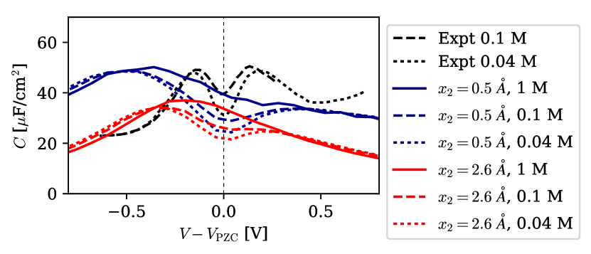
Figure 3: NESS solvation model predicted capacitance for $x_{2}=0.5$ and 2.6 Å, exhibiting both the hump and dip features of the experimental capacitance.

To more conclusively identify the source of the asymmetry in the capacitance curves from the NESS solvation model, we use the electron density results from the NESS calculations as inputs for the $x_{1}$ parameter in our toy model. Fig. 4(a) depicts the induced charge at the Ag(100) surface as a function of applied potential, assigning the distance between the electron density peak and the cavity onset as the $x_{1}^{\mathrm{eff}}$ parameter, plotted in Fig. 4(b) as a function of the electrode surface charge density $\sigma$. Fig. 4(c) depicts the results of the toy model, using the $\sigma$-dependent $x_{1}^{\mathrm{eff}}$ results from Fig. 4(b). The toy model capacitance in Fig. 4(c) and the NESS capacitance of Fig. 3 are in very good agreement, confirming that the asymmetry in the NESS model is caused by the dielectric cavity remaining spatially fixed while the induced charge density shifts with potential.

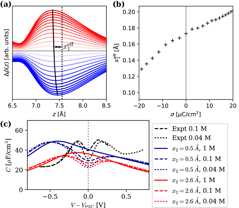
Figure 4: (a) Induced charge density at Ag(100) surface as a function of applied potential, from bottom to top: +0.8 V to -0.8 V relative to the PZC, as in Fig. 3. Dotted line indicates location of dielectric cavity turn-on, and the solid line indicates the maximum of the induced charge density. (b) The separation between these locations in part (a) is the effective vacuum distance, $x_{1}^{\mathrm{eff}}$ between the metal and the solvent as defined in the toy model above, but which now depends on the electrode surface charge density $\sigma$. (c) Capacitance curves predicted by the toy model with this $\sigma$-dependent $x_{1}^{\mathrm{eff}}$.

V Conclusions and Outlook

The NESS solvation model brings the computational electrochemistry community closer to developing an all-purpose solvation model for ions, molecules, and electrified surfaces, but there are still many opportunities for improvement and deeper understanding. For instance, improvements to the dielectric cavity definition and to the dielectric response at the interface have potential to increase accuracy. For the dielectric cavity, the original Soft-Sphere model and NESS employ an atomic radius for each element, currently set based on vdW radii from the UFF force field Rappe et al. (1992). These radii have been carefully evaluated for the few atoms present in organic solutes for which extensive solvation free energy data is readily available. This choice fortuitously gave good results for Ag(100) capacitance, but that might not be the case for all metal surfaces, and for all properties. Additionally, the solvent cavity presently remains fixed with potential and charge on the metal surface; understanding and incorporating the variation of water-metal distance with surface charge could result in further improvements in accuracy for the capacitance. We note that previous solvation models with isodensity cavity parametrizationsJinnouchi and Anderson (2008); Andreussi et al. (2012); Dupont et al. (2013); Fattebert and Gygi (2003); Sundararaman and Goddard (2015); Gunceler et al. (2013); Sundararaman and Schwarz (2017) mitigate some of this asymmetry, but have not yet simultaneously captured solvation energetics and electrochemical capacitance within a single parametrization. Therefore, future work may need to employ a hybrid approach that combines the flexibility of atomic-sphere based cavities with the response to electron density inherent to isodensity cavities. Additionally, for the dielectric response at the interface and near ions, we have assumed that the response of the water remains unchanged from bulk; future improvements could include modulation of the dielectric response adjacent to the solute.

In summary, we find that a solvation model must contain nonlinearities in both the ionic and dielectric responses, along with a region of space containing only the dielectric, in order to capture the features seen in the experimental capacitance curves of metals such as Ag(100) immersed in non-adsorbing electrolytes. By including these characteristics, the NESS solvation model substantially improves on previous solvation models for electrochemical systems, qualitatively capturing key features in the experimental electrochemical capacitance.

VI Supplemental Material

See supplemental information for the convergence of the capacitance with the number of layers of Ag, number of $k$-points, and electron density smearing width. Additionally, the supplemental information contains a discussion of the capacitance behavior of the CANDLE solvation model, and parametrization details of the NESS solvation model developed in this paper.

References

References

- Fried and Boxer (2015) S. D. Fried and S. G. Boxer, Acc. Chem. Res. 48, 998 (2015).
- Fleischmann et al. (1973) M. Fleischmann, P. J. Hendra, and A. J. McQuillan, J. Chem. Soc., Chem. Commun. 0, 80 (1973).
- Wiechers et al. (1988) J. Wiechers, T. Twomey, D. Kolb, and R. Behm, J. Electroanal. Chem. and Interfacial Electrochem. 248, 451 (1988).
- Clavilier (1980) J. Clavilier, J. Electroanal. Chem. 107, 205 (1980).
- Baskin and Prendergast (2017) A. Baskin and D. Prendergast, J. Electrochem. Soc. 164, E3438 (2017).
- Valette (1982) G. Valette, J. Electroanal. Chem. and Interfacial Electrochem. 138, 37 (1982).
- Hamelin (1986) A. Hamelin, in Trends in Interfacial Electrochemistry, Vol. 179, edited by A. Silva (NATO ASI Series, 1986) Chap. 5, pp. 83–102.
- Parsons (1990) R. Parsons, Chem. Rev. 90, 813 (1990).
- Trasatti (1979) S. Trasatti, Mod. Aspects Electrochem. 13, 81 (1979).
- Damaskin and Frumkin (1974) B. Damaskin and A. Frumkin, Electrochim. Acta 19, 173 (1974).
- Stern (1924) O. Stern, Z. Elektrochem. Angew. Phys. Chem. 30, 508 (1924).
- Grahame (1947) D. Grahame, Chem. Rev. 41, 441 (1947).
- Parsons and Zobel (1965) R. Parsons and F. Zobel, J. Electroanal. Chem. 9, 333 (1965).
- Schmickler and Henderson (1986) W. Schmickler and D. Henderson, J. Chem. Phys. 85, 1650 (1986).
- Saradha and Sangaranarayanan (1998) R. Saradha and M. Sangaranarayanan, J. Phys. Chem. B 102, 5468 (1998).
- Amokrane and Badiali (1992) S. Amokrane and J. Badiali, in Modern Aspects of Electrochemistry, Number 22, edited by Bockris (1992).
- Markovich et al. (2014) T. Markovich, D. Andelman, and R. Podgornik, in Handbook of Lipid Membranes: Molecular, Functional, and Materials Aspects, edited by C. Safinya and J. Radler (Taylor & Francis, 2014) Chap. 9.
- Xiao et al. (2016) H. Xiao, T. Cheng, W. A. Goddard III, and R. Sundararaman, J. Am. Chem. Soc. 138, 483 (2016).
- Jason D. Goodpaster and Head-Gordon (2016) A. T. B. Jason D. Goodpaster and M. Head-Gordon, J. Phys. Chem. Lett. 7, 1471 (2016).
- Garza et al. (2018) A. J. Garza, A. T. Bell, and M. Head-Gordon, J. Phys. Chem. Lett. 9, 601 (2018).
- Fisicaro et al. (2017) G. Fisicaro, L. Genovese, O. Andreussi, S. Mandal, N. N. Nair, N. Marzari, and S. Goedecker, J. Chem. Theory Comput. 13, 3829 (2017).
- Gunceler et al. (2013) D. Gunceler, K. Letchworth-Weaver, R. Sundararaman, K. A. Schwarz, and T. A. Arias, Modell. and Simul. Mat. Sci. Eng. 21, 074005 (2013).
- Letchworth-Weaver and Arias (2012) K. Letchworth-Weaver and T. A. Arias, Phys. Rev. B 86, 075140 (2012).
- Mathew et al. (2014) K. Mathew, R. Sundararaman, K. Letchworth-Weaver, T. A. Arias, and R. G. Hennig, J. Chem. Phys. 140 (2014).
- Sundararaman and Goddard (2015) R. Sundararaman and W. Goddard, J. Chem. Phys 142, 064107 (2015).
- Andreussi et al. (2012) O. Andreussi, I. Dabo, and N. Marzari, J. Chem. Phys 136, 064102 (2012).
- Dupont et al. (2013) C. Dupont, O. Andreussi, and N. Marzari, J. Chem. Phys 139, 214110 (2013).
- Jinnouchi and Anderson (2008) R. Jinnouchi and A. Anderson, Phys. Rev. B 77, 245417 (2008).
- Dabo et al. (2010) I. Dabo, Y. Li, N. Bonnet, and N. Marzari, in Fuel Cell Science: Theory, Fundamentals, and Biocatalysis, edited by A. Wieckowski and J. Norskov (Wiley, 2010) Chap. 13.
- Sundararaman and Schwarz (2017) R. Sundararaman and K. Schwarz, J. Chem. Phys. 146, 084111 (2017).
- Tomasi et al. (2005) J. Tomasi, B. Mennucci, and R. Cammi, Chem. Rev. 105, 2999 (2005).
- Marenich et al. (2009) A. V. Marenich, C. J. Cramer, and D. G. Truhlar, J. Phys. Chem. B 113, 6378 (2009).
- Sundararaman et al. (2017a) R. Sundararaman, W. A. Goddard III, and T. A. Arias, J. Chem. Phys. 146, 114104 (2017a).
- Sundararaman et al. (2017b) R. Sundararaman, K. Letchworth-Weaver, K. Schwarz, D. Gunceler, Y. Ozhabes, and T. A. Arias, SoftwareX 6, 278 (2017b).
- Perdew et al. (1996) J. P. Perdew, K. Burke, and M. Ernzerhof, Phys. Rev. Lett. 77, 3865 (1996).
- Garrity et al. (2014) K. F. Garrity, J. W. Bennett, K. Rabe, and D. Vanderbilt, Comput. Mater. Sci. 81, 446 (2014).
- Sundararaman and Arias (2013) R. Sundararaman and T. Arias, Phys. Rev. B 87, 165122 (2013).
- Sundararaman et al. (2014) R. Sundararaman, K. Letchworth-Weaver, and T. A. Arias, J . Chem. Phys. 140, 144504 (2014).
- Marcus (1988) Y. Marcus, Chem. Rev. 88, 1475 (1988).
- Roobottom et al. (1999) H. K. Roobottom, H. D. B. Jenkins, J. Passmore, and L. Glasser, J. Chem. Ed. 76, 1570 (1999).
- Trasatti (1983) S. Trasatti, J. Electroanal. Chem. 150, 1 (1983).
- Valette (1981) G. Valette, J. Electroanal. Chem. 122, 285 (1981).
- Sundararaman and Arias (2014) R. Sundararaman and T. Arias, Comp. Phys. Comm. 185, 818 (2014).
- Rappe et al. (1992) A. K. Rappe, C. J. Casewit, K. S. Colwell, I. Goddard, W. A., and W. M. Skiff, J. Am. Chem. Soc. 114, 10024 (1992).
- Fattebert and Gygi (2003) J. L. Fattebert and F. Gygi, Int. J. Quantum Chem. 93 (2003).