[1801.07671] INTRODUCTION

Astronomy Letters, 2018, Vol. 44, No 3, pp. 193–201.

Search for Stellar Streams Based on Data from

the RAVE5 and Gaia TGAS Catalogues

A.T. Bajkova¹¹1e-mail: anisabajkova@gao.spb.ru and V.V. Bobylev

Pulkovo Astronomical Observatory, Russian Academy of Sciences,

Pulkovskoe sh. 65, St. Petersburg, 196140 Russia

Abstract—We have analyzed the space velocities of stars with the proper motions and trigonometric parallaxes from the Gaia TGAS catalogue in combination with the line-of-sight velocities from the RAVE5 catalogue. In the $V,\sqrt{U^{2}+2V^{2}}$ velocity plane we have identified three clumps, BB17-1, BB17-2, and BB17-3, in the region of large velocities ( $V<-150$ km s^-1). The stars of the BB17-1 and BB17-2 clumps are associated with the kinematic groups VelHel-6 and VelHel-7 detected previously by Helmi et al. We give the greatest attention to the BB17-3 clump. The latter is shown to be most closely linked with the debris of the globular cluster $\omega$ Cen. In the BB17-3 clump we have identified 28 stars with a low velocity dispersion with respect to the center of their distribution. All these stars have very close individual age estimates: $\log t\approx 10$ . The distribution of metallicity indices in this sample is typical for the stars of the globular cluster $\omega$ Cen. In our opinion, the BB17-3 clump can be described as a homogeneous stream in the debris of the cluster $\omega$ Cen.

DOI: 10.1134/S1063773718020019

INTRODUCTION

A study of the ellipsoidal distribution of stellar space velocities as a function of stellar age led to an understanding of the dynamical properties of the Galaxy and its subsystems. The observed velocity distribution turned out to be nonuniform (Eggen 1958, 1996).

The fine structure of the velocity field manifests itself in different planes. An analysis of the rectangular $U,V,W$ velocities is most popular. Even in the region of relatively small (up to $\sim$ 40 km s^-1) $U$ and $V$ velocities there are known peaks named after their association with open star clusters (OSCs), such as the Pleiades, Sirius, Coma Berenices, or the Hyades (Eggen 1958, 1996). It was suggested to associate a number of peaks with older open star clusters and stellar groups in the Galactic disk, for example, Wolf 630, 61 Cygni (Eggen 1969), $\zeta$ Herculis, $\sigma$ Puppis, or $\varepsilon$ Indi (Eggen 1971a).

According to the theory of stellar streams (Eggen 1996), the peaks reflect the presence of tubes or stellar debris, OSC debris, in circumsolar space. Such debris must be formed during the disruption of clusters under the influence of Galactic tides, giant molecular clouds, and other gravitational perturbations. The debris gradually extend along the Galactic orbit of clusters and are completely mixed with the stellar Galactic background 1–2 Gyr later. The presence of debris is confirmed by numerical simulations of the dynamical evolution of OSCs (Chumak et al. 2005; Chumak and Rastorguev and 2006a, 2006b).

An analysis of the stellar velocities from the Hipparcos (1997) catalogue showed that, in addition to the already known peaks, the two-dimensional distribution of $UV$ velocities has a more complex structure. Specifically, there are several extended “branches” located almost parallel to one another (Skuljan et al. 1999).

Apart from the branches, bimodality of the distribution manifests itself in the $UV$ velocity plane (Dehnen 1998, 2000). Such a velocity stratification can be caused by resonance effects. In particular, the formation of the $\zeta$ Herculis ( $V\approx-50$ km s^-1) and Wolf 630 ( $V\approx-20$ km s^-1, $U\approx 40$ km s^-1) streams can be explained by the resonances produced by the central Galactic bar (Dehnen 2000; Fux 2001).

Tidal tails have been detected in a number of globular clusters (Grillmair et al. 1995; Leon et al. 2000; Odenkirchen et al. 2001; Belokurov et al. 2006; Sollima et al. 2011; Navarrete et al. 2017) and dwarf galaxies, satellites of the Milky Way Galaxy (Ibata et al. 2001; Grillmair and Dionatos 2006; Helmi 2008). Some of the observed clumps of stellar $UV$ velocities in the solar neighborhood at velocities $V<-100$ km s^-1 are associated with such debris. For example, these include the Arcturus (Eggen 1971b) and KFR08 (Klement et al. 2008) streams. It is suggested that several stellar streams with high velocities $V<-150$ km s^-1 consisting of extremely metal-poor stars recently discovered by Helmi et al. (2017) are the debris of disrupted satellite galaxies. In the opinion of these authors, most of the detected streams are associated with the debris of the globular cluster $\omega$ Cen.

The goal of this study is to analyze the stellar velocity field in the solar neighborhood to reveal stellar groups with a common dynamical origin. We focus our attention on the stars with large velocities relative to the Sun and, as a rule, these are fairly old, metalpoor stars. For our analysis we use the positions, proper motions, and trigonometric parallaxes from the Gaia DR1 catalogue (Gaia Collaboration, Prusti et al. 2016) in combination with the line-of-sight velocities from the RAVE (RAdial Velocity Experiment) catalogue (Steinmetz et al. 2006).

DATA

The observations within the RAVE project have been performed since 2003 in the Southern Hemisphere at the 1.2-m Schmidt telescope of the Anglo-Australian Observatory. Five releases of the catalogue have been published. The mean line-of-sight velocity error is about 3 km s^-1. The RAVE5 version (Kunder et al. 2017) contains data on 457 588 stars; more than 200 000 of them are common to the first published version of the Gaia catalogue.

This version was produced from a combination of the data in the first year of orbital Gaia satellite observations with the Tycho-2 stellar positions (Hog et al. 2000). It is designated as TGAS (Tycho.Gaia Astrometric Solution; Brown et al. 2016; Lindegren et al. 2016) and contains the positions, trigonometric parallaxes, and proper motions of $\sim$ 2 million stars. For $\sim$ 90 000 stars common to the Hipparcos (1997) catalogue the mean random error of their proper motions is $\sim$ 0.06 mas yr^-1 (milliarcseconds per year); for the remaining stars this error is $\sim$ 1 mas yr^-1 (Brown et al. 2016).

METHOD

We know three stellar velocity components from observations: the line-of-sight velocity $V_{r}$ and the two velocity components $V_{l}=4.74r\mu_{l}\cos b$ and $V_{b}=4.74r\mu_{b}$ along the Galactic longitude $l$ and latitude $b$ expressed in km s^-1. The proper motion components $\mu_{l}\cos b$ and $\mu_{b}$ are expressed in mas yr^-1. The coefficient 4.74 is the ratio of the number of kilometers in an astronomical unit to the number of seconds in a tropical year, and $r$ is the stellar heliocentric distance in kpc. In this paper the distances are calculated using the trigonometric parallaxes from the Gaia TGAS catalogue and, therefore, $r=1/\pi.$ The $U,V,W$ velocities along the rectangular Galactic $x,y,z$ coordinate axes are calculated via the $V_{r},V_{l},V_{b}$ components:

\begin{array}[]{lll}U=V_{r}\cos l\cos b-V_{l}\sin l-V_{b}\cos l\sin b,\\ V=V_{r}\sin l\cos b+V_{l}\cos l-V_{b}\sin l\sin b,\\ W=V_{r}\sin b+V_{b}\cos b.\end{array}

(1)

where the velocity $U$ is directed from the Sun to the Galactic center, $V$ is in the direction of Galactic rotation, and $W$ is directed to the North Galactic Pole. To extract the statistically significant signals of nonuniformities in the distributions of $UV$ velocities, we use the wavelet transform known as a powerful tool for filtrating spatially localized signals (Chui 1997; Vityazev 2001). The wavelet transform of the two dimensional distribution $f(U,V)$ consists in its decomposition into analyzing wavelets $\psi(U/a,V/a)$ , where $a$ is the coefficient that allows the wavelet of a certain scale to be extracted from the entire family of wavelets characterized by the same shape $\psi$ . The wavelet transform $w(\xi,\eta)$ is defined as a correlation function in such a way that at any given point $(\xi,\eta)$ in the $UV$ plane we have one real value of the following integral:

\begin{array}[]{ccc}\displaystyle w(\xi,\eta)=\int_{-\infty}^{\infty}\int_{-\infty}^{\infty}f(U,V)\psi\Biggl{(}\displaystyle\frac{(U-\xi)}{a},\frac{(V-\eta)}{a}\Biggr{)}dUdV,\end{array}

(2)

which was called the wavelet coefficient at point $(\xi,\eta)$ . Obviously, in the case of finite discreet maps that we deal with, their number is finite and equal to the number of square bins on the map.

Refer to caption — Figure 1: Wavelet map of the $V,\sqrt{U^{2}+2V^{2}}$ velocity plane. The stellar velocities are given relative to the Sun.

As the analyzing wavelet we use a traditional wavelet called the Mexican HAT (MHAT). The two-dimensional MHAT wavelet is described by the expression

\psi(d/a)=\Biggl{(}2-\frac{d^{2}}{a^{2}}\Biggr{)}e^{-d^{2}/2a^{2}},

(3)

where $d^{2}=U^{2}+V^{2}$ . The wavelet (3) is obtained from differentiating the Gaussian function twice. The main property of the function $\psi$ is that its integral over $U$ and $V$ is zero, which allows any nonuniformities in the distribution being studied to be detected. If the distribution being analyzed is uniform, then all coefficients of the wavelet transform will be zero.

To select the candidates without significant random observational errors, we took the stars satisfying the following criteria:

\begin{array}[]{ccc}|V_{r}|<350~{}{\hbox{\rm km s${}^{-1}$}},\\ \sigma_{V_{r}}<5~{}{\hbox{\rm km s${}^{-1}$}},\\ \sigma_{\mu_{\alpha}\cos\delta}<10~{}{\hbox{\rm mas yr${}^{-1}$}},\\ ~{}~{}~{}~{}\sigma_{\mu_{\delta}}<10~{}{\hbox{\rm mas yr${}^{-1}$}},\\ \sigma_{\pi}/\pi<0.5.\end{array}

(4)

More than 200 000 stars with the trigonometric parallaxes and proper motions from the Gaia TGAS catalogue and the line-of-sight velocities from the RAVE5 catalogue satisfy these constraints. The constraint on the magnitude of the line-of-sight velocity $|V_{r}|$ is related to the existence of an appreciable number of low-quality measurements (with low signal-to noise ratios) with line-of-sight velocities exceeding the threshold escape velocity from the Galaxy.

Table 1: Data on the stars of the BB17-3 clump

TYC	$l,$ deg.	$b,$ deg.	$T_{\hbox{\tiny\rm eff}},$ K	$\log~{}$ g	[M/H], dex	$\pi_{Gaia},$ mas	$\log t$
8004-1288-1	$1.4$	$-62.5$	5212	2.94	$-1.83\pm 0.18$	$0.67\pm 0.33$	$10.00\pm 0.05$
7954-0027-1	$1.8$	$-36.7$	5076	2.76	$-1.86\pm 0.18$	$1.07\pm 0.32$	$9.99\pm 0.07$
6989-0218-1	$4.8$	$-78.1$	4993	2.72	$-0.85\pm 0.09$	$1.95\pm 0.41$	$9.89\pm 0.22$
7442-1834-1	$11.9$	$-32.0$	5801	0.78	$-0.47\pm 0.09$	$5.35\pm 0.29$
6900-0414-1	$14.8$	$-27.1$	5725	3.98	$-2.12\pm 0.26$	$1.26\pm 0.29$	$9.98\pm 0.12$
6410-0404-1	$48.2$	$-73.1$	4931	2.13	$-1.59\pm 0.14$	$1.52\pm 0.34$	$9.99\pm 0.07$
4696-0131-1	$171.8$	$-62.2$	5931	3.87	$-1.06\pm 0.19$	$3.53\pm 0.30$	$9.93\pm 0.20$
7028-0807-1	$229.0$	$-52.5$	5457	2.73	$-2.35\pm 0.27$	$0.86\pm 0.28$	$10.01\pm 0.06$
7042-1158-1	$236.3$	$-41.5$	4962	1.86	$-1.36\pm 0.17$	$1.61\pm 0.25$	$9.99\pm 0.11$
7018-0652-1	$238.2$	$-62.0$	5109	3.60	$-1.01\pm 0.19$	$2.58\pm 0.23$	$9.91\pm 0.19$
6520-0236-1	$239.0$	$-15.0$	4985	1.87	$-1.33\pm 0.17$	$0.94\pm 0.31$	$9.88\pm 0.28$
8075-0797-1	$257.5$	$-43.9$	4031	0.55	$-1.23\pm 0.14$	$0.62\pm 0.27$	$10.00\pm 0.08$
8890-0860-1 *	$276.5$	$-34.1$	3800	1.00	$0.00\pm 0.10$	$1.25\pm 0.45$
8048-0222-1	$277.4$	$-62.3$	4655	0.82	$-2.03\pm 0.14$	$1.02\pm 0.32$	$10.00\pm 0.05$
6658-1026-1	$279.8$	$32.2$	5434	3.05	$-1.31\pm 0.18$	$4.31\pm 0.43$
6656-0054-1	$282.0$	$34.9$	5500	3.77	$-2.15\pm 0.26$	$3.54\pm 0.36$	$10.00\pm 0.08$
9152-1687-1	$285.6$	$-41.5$	5659	4.74	$-2.10\pm 0.26$	$2.80\pm 0.29$	$10.00\pm 0.10$
8227-1820-1	$291.6$	$9.2$	4794	0.80	$-2.82\pm 0.14$	$0.70\pm 0.26$	$10.00\pm 0.06$
4954-0606-1	$296.1$	$56.3$	5038	1.74	$-1.54\pm 0.17$	$1.30\pm 0.49$	$10.00\pm 0.12$
8852-0851-1	$298.1$	$-53.8$	5055	4.39	$-2.04\pm 0.26$	$0.77\pm 0.25$	$9.99\pm 0.10$
8473-0759-1	$300.4$	$-63.4$	4836	2.44	$-0.62\pm 0.09$	$1.13\pm 0.24$	$9.76\pm 0.25$
6112-0045-1	$308.7$	$46.9$	5846	3.56	$-2.33\pm 0.26$	$2.59\pm 0.92$	$10.00\pm 0.07$
9032-2385-1	$314.6$	$-6.3$	4921	1.97	$-1.33\pm 0.17$	$1.36\pm 0.34$	$9.78\pm 0.40$
8821-0626-1	$333.3$	$-48.3$	5750	3.21	$-1.32\pm 0.18$	$0.62\pm 0.26$	$9.99\pm 0.15$
8828-0140-1	$333.4$	$-49.4$	6000	3.50	$-0.75\pm 0.08$	$1.12\pm 0.48$	$9.85\pm 0.21$
4977-1226-1	$343.6$	$52.9$	5033	2.55	$-1.08\pm 0.17$	$1.11\pm 0.28$	$9.85\pm 0.35$
8401-0199-1	$346.6$	$-27.1$	4625	1.39	$-1.21\pm 0.17$	$0.97\pm 0.26$
8389-1156-1	$352.1$	$-26.4$	4713	0.97	$-1.78\pm 0.17$	$1.21\pm 0.25$	$9.99\pm 0.10$

(*) This star cannot be found by its Tycho number in the SIMBAD electronic database, but it has an alternative designation, RAVE J051701.4 $-$ 661815.

RESULTS

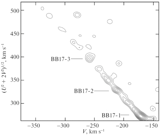
To identify the low-power clumps in the region of high space velocities, we apply the approach proposed by Arifyanto and Fuchs (2006). For this purpose, we consider the distribution of stellar velocities in the $V,\sqrt{U^{2}+2V^{2}}$ plane. Using this approach, Klement et al. (2008) discovered the KFR08 stream, while Bobylev et al. (2010) found new bright members of this stream.

Figure 1 presents the wavelet map of the $V,\sqrt{U^{2}+2V^{2}}$ velocity plane constructed using the same stars as those in the previous step. The three BB17-1, BB17-2, and BB17-3 clumps now manifest themselves especially clearly, while the BB17-3 clump appears as a completely isolated peak. Interestingly, in Fig. 5 from Bobylev et al. (2010) constructed using Hipparcos data we can see low-power clumps of stars near the BB17-2 ( $V=-220$ km s^-1, $\sqrt{U^{2}+2V^{2}}=330$ km s^-1) and BB17-3 ( $V=-270$ km s^-1, $\sqrt{U^{2}+2V^{2}}=390$ km s^-1) peaks.

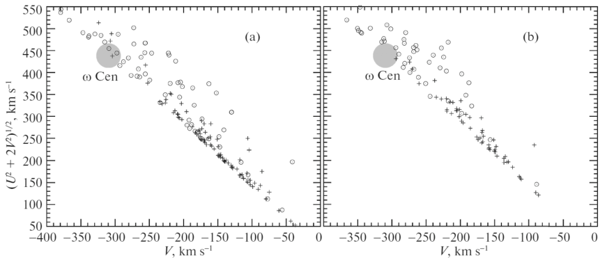
The velocity distribution of low-metallicity stars in the $V,\sqrt{U^{2}+2V^{2}}$ plane for nine groups whose list was taken from Helmi et al. (2017) is shown in Fig. 2. Here we want to show that the positions of the stars from the VelHel-1, 2, 3, 4, 5, 8, and 9 groups are fairly close to the position of the globular cluster $\omega$ Cen.

Note that Helmi et al. (2017) searched for the groups by analyzing the integrals of motion, i.e., based on a technique different from ours. Moreover, they used the photometric distances from the RAVE5 catalogue, because their goal was to analyze the stars sufficiently far from the Sun, $r>100$ pc. To construct Fig. 2, we calculated the stellar velocities using both the trigonometric parallaxes (while ignoring the constraints (4)) and the photometric distances by taking into account the constraints (4).

The position of the globular cluster $\omega$ Cen in this figure is marked by the circle whose size exceeds considerably the random measurement errors of the cluster velocities. Although the radius of this circle is arbitrary, we wish to emphasize that there is a noticeable velocity dispersion in the cluster and its debris. According to the determinations by Sollima et al. (2009), the stellar velocity dispersion at the center of the cluster $\omega$ Cen is about 17.2 km s^-1 and reaches approximately 5.2 km s^-1, but then remains at a level of 7–8 km s^-1 for a long time at increasingly large distances from the cluster center.

According to Helmi et al. (2017), the VelHel-6 and VelHel-7 groups are not associated with the debris of the globular cluster $\omega$ Cen. As can be seen from Fig. 2a, most of the crosses are concentrated near $V=-170$ km s^-1 and $\sqrt{U^{2}+2V^{2}}=250$ km s^-1, but rare crosses are also encountered in the upper part of the diagram, while open circles are encountered in its lower part. A considerably larger concentration of open circles to the position of $\omega$ Cen and a tighter concentration of crosses to the BB17-1 and BB17-2 peaks (Fig. 1) are clearly seen in Fig. 2b. We can conclude that the results of our selection of stars based on a fairly simple technique agree well with the results of applying the method based on the calculation of the integrals of motion.

We determined the significance level of the revealed peaks by the method of Monte Carlo simulations as described in Skuljan et al. (1999). For this purpose, we generated $M=10000$ random realizations of $(U,V)$ velocities by taking into account their measurement errors. We assumed the errors to be additive and to be distributed according to a normal law with zero mean and a dispersion equal to the measurement error. For each random realization we constructed a wavelet map and determined whether there was a clump in the region of the revealed peaks. The ratio of the number $N$ of realizations that show the presence of peaks to the total number $M$ of random realizations gives the significance level of the peaks. In our case, the significance level of the new revealed peaks was approximately 91%. This means that the detected clumps may be deemed real rather than generated by random noise with a probability of about 91%.

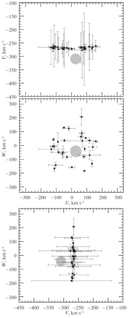
The stellar velocity distribution for the BB17-3 stream in the $UV,$ $UW,$ and $VW$ planes is presented in Fig. 3; the position of the globular cluster $\omega$ Cen is marked by the circle of an arbitrary size. Note the $UW$ velocity plane, in which the velocity dispersions in both coordinates, $\sigma_{U}$ and $\sigma_{W}$ , are seen to be equal; however, here we can say nothing about the dispersion $\sigma_{V}$ because of the peculiarities of our selection of stars.

It is well known that an isotropic (Maxwellian) velocity distribution takes place in spherically symmetric systems, for example, in globular clusters. At present, the isotropy of the velocity dispersion has been measured quite reliably for several globular clusters (Watkins et al. 2015) by invoking the Hubble Space Telescope observations of stellar proper motions. The mean ratio of the velocity dispersions in the tangential and radial directions at the cluster center calculated from the data on 22 globular clusters is $\sigma_{t}/\sigma_{r}=0.992\pm 0.005$ , while for the globular cluster $\omega$ Cen this ratio is $\sigma_{t}/\sigma_{r}=1.01\pm 0.01$ .

The velocity dispersion in the debris, of course, will be larger than that in the parent cluster or galaxy, but the main properties must be retained. It is also assumed that the stars in the debris must have a homogeneous chemical composition owing to their common origin.

The stars of the BB17-3 stream that we selected are listed in the table. Column 1 gives the numbers according to the Tycho-2 catalogue; columns 2 and 3 give the Galactic coordinates $l,b;$ columns 4–6 give the effective temperature $T_{\hbox{\tiny\rm eff}},$ gravity $\log~{}$ g, and metallicity [M/H] copied from the RAVE5 catalogue; the next-to-last column gives the trigonometric parallax $\pi_{Gaia}$ ; and the last column gives the individual age estimate copied from the RAVE4 catalogue (Kordopatis et al. 2013). Note that the influence of the well-known Lutz–Kelker bias (Lutz and Kelker 1973) is negligible at small $\sigma_{\pi}/\pi$ (10–15%); otherwise, this bias should be taken into account (Stepanishchev and Bobylev 2013; Astraatmadja and Bailer-Jones 2017). As can be seen from the table, the selected stars mostly have an acceptable mean level of errors $\sigma_{\pi}/\pi$ , which do not exceed 0.27. In addition, the entire group is very homogeneous in age.

In fact, we selected the stars based on the boundaries of the corresponding peak in Fig. 1. For this purpose, we took the stars in a square with a $V$ side from $-$ 258 km s^-1 to $-$ 278 km s^-1 and a $\sqrt{U^{2}+2V^{2}}$ side from 380 to 405 km s^-1. Our list has no stars common to both the groups of probable members of the $\omega$ Cen stream proposed by Helmi et al. 2017) and the list of probable bright members of this stream from Navarrete et al. (2015). Note that Helmi et al. (2017) selected the candidates with metallicities [M/H] $\leq-1.5,$ typical for the lowest-metallicity halo stars. As can be seen from the table, the metallicities of our selected stars lie in the range [M/H] $\leq$ 0. On the whole, this is consistent with the spectroscopic analysis of stars in the globular cluster $\omega$ Cen by Gratton et al. (2011), who established the presence of several populations with different chemical compositions in this cluster. As Villanova et al. (2014) showed, the subgiants in the globular cluster $\omega$ Cen form five populations with different metallicities, a mean age of $\sim$ 10 Gyr, and a dispersion around this value of $\sim$ 2 Gyr.

At the same time, such metallicities and ages are typical for halo stars (Jofré and Weiss 2011). Therefore, we cannot separate the halo stars from the stars of the $\omega$ Cen debris in our sample of BB17-3 clump stars based on their metallicities and ages.

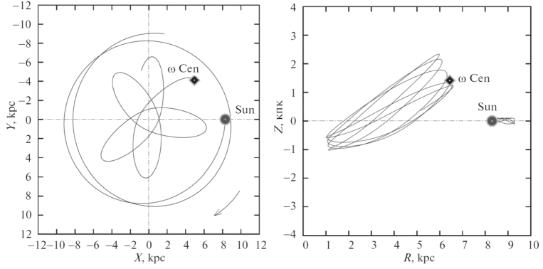
Figure 4 presents the Galactic orbits of the Sun and the globular cluster $\omega$ Cen constructed in an interval of 400 Myr into the future. The following input parameters taken from the SIMBAD electronic astronomical database were used for the cluster $\omega$ Cen: $\alpha=201^{\circ}.69165,$ $\delta=-47^{\circ}.47694,$ $\mu_{\alpha}\cos\delta=-6.01\pm 0.25$ mas yr^-1, $\mu_{\delta}=-5.02\pm 0.25$ mas yr^-1, $V_{r}=238\pm 5$ km s^-1, and $d=5.5\pm 0.2$ kpc. The peculiar velocity of the Sun relative to the local standard of rest was assumed to be $(u_{\odot},v_{\odot},w_{\odot})=(11.1,12.2,7.3)$ km s^-1, as determined by Schönrich et al. (2010). To construct the Galactic orbits of the Sun and the globular cluster $\omega$ Cen, we used the axisymmetric three-component model of the Galactic potential with parameters from Bajkova and Bobylev (2016), where it is designated as model III. The debris of constructing the Galactic orbits of globular clusters are described in Bobylev and Bajkova (2017). It can be seen from Fig. 4 that the Sun’s motion is prograde (coincides in direction with the Galactic one), while the motion of the cluster $\omega$ Cen is retrograde. There is good agreement of our constructed orbit with the results of other authors, for example, the orbits from Mizutani et al. (2003) or Majewski et al. (2012) constructed using other models of the Galactic gravitational potential.

DISCUSSION AND CONCLUSIONS

Let us first say a few words about the main characteristics of the cluster $\omega$ Cen. Among all of the known globular clusters in the Galaxy, $\omega$ Cen is one of the biggest. Indeed, it has the largest size, the greatest oblateness $\varepsilon=0.17$ (Watkins et al. 2015), the highest luminosity, and the largest mass, whose estimates lie in the range from $5\times 10^{6}M_{\odot}$ (Meylan et al. 1995) to $2.5\times 10^{6}M_{\odot}$ (van de Ven et al. 2006). Thus, this cluster contains several million stars, but it can also lose many stars because of the tidal effect of the Galaxy, especially since the pericenter of the cluster orbit is very close to the Galactic center (Fig. 4).

(1) An examination of Fig. 4 leads to the question of precisely how the stars of the $\omega$ Cen debris ended up in the solar neighborhood. After all, to reach the solar circle, these stars should traverse approximately 2 kpc in the radial direction.

Note, for example, the results of numerical simulations of the dynamical evolution of the globular cluster Note, for example, the results of numerical simulations of the dynamical evolution of the globular cluster $\omega$ Cen and the formation of its debris obtained by Ideta and Makino (2004). As these authors showed, already $\sim$ 0.44 Gyr after the start time of the dwarf galaxy’s disruption, the width of its debris in the radial direction was $\sim$ 4 kpc in some places, while after 0.88 Gyr the debris fills the solar circle almost completely. In these simulations the initial mass of the dwarf progenitor galaxy was $1.3\times 10^{8}M_{\odot}$ and it was located at an initial distance of $\sim$ 6 kpc from the center of the Milky Way.

The results by Meza et al. (2005), who studied the debris of the origin of a series of debris formed through multiple periodic encounters of the dwarf progenitor galaxy of the globular cluster $\omega$ Cen with the Milky Way, are even more interesting. Based on numerical simulations, these authors showed that during each encounter the dwarf galaxy left stars with different energies and angular momenta in the corresponding debris. The debris were preserved at different Galactocentric distances. Therefore, a present day observer sees such stars as different kinematic streams. In these simulations the initial mass of the dwarf galaxy was $4.6\times 10^{9}M_{\odot}$ and it was located at an initial distance of 140 kpc from the center of the Milky Way and moved in a highly elliptical orbit.

Mizutani et al. (2003) modeled the kinematic properties of the tidal disruption of a dwarf galaxy in the attractive field of the Milky Way. The central part of the dwarf galaxy was assumed to contain the globular cluster $\omega$ Cen. The motion of the dwarf galaxy was traced in a long time interval in the past, 1.5–1.9 Gyr, using several models. They confirmed that the motion of the series of formed debris is retrograde. A strong concentration of debris stars near the solar circle was found in one of the models (model 2).

Majewski et al. (2012) pointed that their selected candidates are concentrated in the fourth Galactic quadrant. Their simulations showed that most stars from the $\omega$ Cen debris are located within the solar circle and are concentrated in the fourth quadrant, near the current position of this cluster. Note that a similar conclusion follows from an analysis of the Galactic coordinates for the stars in our table.

(2) All of the identified 28 stars in the BB17-3 clump have very close ages. The distribution of their metallicity indices resembles that observed for the stars of the globular cluster $\omega$ Cen. For example, looking at Fig. 2b, we can conclude that the stars covering almost the entire upper left corner of the diagram, i.e., filling the square with a $V$ side from $-250$ to $-200$ km s^-1 and a $\sqrt{U^{2}+2V^{2}}$ side from 350 to 500 km s^-1, belong to the $\omega$ Cen debris. The stars in this square are distributed quite uniformly. However, as can be seen from Fig. 1, the 28 stars of the BB17-3 clump form a separate peak clearly visible by the unaided eye. We can assume with a high probability that these stars belong to the debris of the cluster $\omega$ Cen. We also get the impression that they can belong to a fairly homogeneous “stream” in the cluster debris.

(3) The positions of the BB17-1 and BB17-2 peaks agree well with the positions of the VelHel-6 and VelHel-7 streams (if, for example, Fig. 1 and Fig. 2b are compared) found by Helmi et al. (2017). In fact, the presence of two such streams was confirmed in this paper. At present, no specific cluster or galaxy that could form debris or streams with such characteristics has been proposed. Therefore, searching for such objects can become an interesting task in future.

We can conclude that in this paper the greatest attention is given to the BB17-3 clump. We showed that it is most closely linked with the debris of the globular cluster $\omega$ Cen. In this clump we identified 28 stars having a low velocity dispersion with respect to the center of their distribution in the $V,\sqrt{U^{2}+2V^{2}}$ plane. The list of BB17-3 clump members does not overlap with the list of members of the VelHel-1, 2, 3, 4, 5, 8, and 9 groups described by Helmi et al. (2017) and also associated with the debris of the globular cluster $\omega$ Cen. All these stars have very close individual age estimates, $\log t\approx 10$ . The distribution of metallicity indices in this sample is typical for the stars of the globular cluster $\omega$ Cen. In our opinion, the 28 stars of the BB17-3 clump can be characterized as a homogeneous stream in the extended debris of the cluster $\omega$ Cen.

ACKNOWLEDGMENTS

We are grateful to the referee for the useful remarks that contributed to an improvement of the paper. This work was supported by the Basic Research Program P–7 of the Presidium of the Russian Academy of Sciences, the “Transitional and Explosive Processes in Astrophysics” Subprogram. In our study we used the SIMBAD electronic database.

REFERENCES

1. M. I. Arifyanto and B. Fuchs, Astron. Astrophys. 449, 533 (2006).

2. T. L. Astraatmadja and C. A. L. Bailer-Jones, Astrophys. J. 833, 119 (2017).

3. A. T. Bajkova and V. V. Bobylev, Astron. Lett. 42, 567 (2016).

4. V. Belokurov, N. W. Evans, M. J. Irwin, P. C. Hewett, and M. I. Wilkinson, Astrophys. J. 637, L29 (2006).

5. V. V. Bobylev, A. T. Bajkova, and A. A. Mylläri, Astron. Lett. 36, 27 (2010).

6. V. V. Bobylev and A. T. Bajkova, Astron. Rep. 61, 551 (2017).

7. A. G. A. Brown, A. Vallenari, T. Prusti, J. de Bruijne, F. Mignard, R. Drimmel, C. Babusiaux, et al. (GAIA Collab.), Astron. Astrophys. 595, 2 (2016).

8. C. K. Chui, Wavelets: A Mathematical Tool for Signal Analysis (SIAM, Philadelphia, PA, 1997).

9. Ya. O. Chumak, A. S. Rastorguev, and S. D. Arset, Astron. Lett. 31, 308 (2005).

10. Ya. O. Chumak and A. S. Rastorguev, Astron. Lett. 32, 157 (2006a).

11. Ya. O. Chumak and A. S. Rastorguev, Astron. Lett. 32, 446 (2006b).

12. W. Dehnen, Astron. J. 115, 2384 (1998).

13. W. Dehnen, Astron. J. 119, 800 (2000).

14. O. J. Eggen, Mon. Not. R. Astron. Soc. 118, 65 (1958).

15. O. J. Eggen, Publ. Astron. Soc. Pacif. 81, 553 (1969).

16. O. J. Eggen, Publ. Astron. Soc. Pacif. 83, 251 (1971a).

17. O. J. Eggen, Publ. Astron. Soc. Pacif. 83, 271 (1971b).

18. O. J. Eggen, Astron. J. 112, 1595 (1996).

19. R. Fux, Astron. Astrophys. 373, 511 (2001).

20. R. G. Gratton, C. I. Johnson, S. Lucatello, V. DÓrazi, and C. Pilachowski, Astron. Astrophys. 534, 72 (2011).

21. C. J. Grillmair, K. C. Freeman, M. Irwin, and P. J. Quinn, Astron. J. 109, 2553 (1995).

22. C. J. Grillmair, and O. Dionatos, Astrophys. J. Lett. 651, L29 (2006).

23. A. Helmi, Astron. Astrophys. Rev. 15, 145 (2008).

24. A. Helmi, J. Veljanoski, M. A. Breddels, H. Tian, and L. V. Sales, Astron. Astrophys. 598, 58 (2017).

25. E. Hog, C. Fabricius, V. V. Makarov, U. Bastian, P. Schwekendiek, A. Wicenec, S. Urban, T. Corbin, and G. Wycoff, Astron. Astrophys. 355, L27 (2000).

26. R. Ibata, M. Irwin, G. F. Lewis, and A. Stolte, Astrophys. J. 547, L133 (2001).

27. M. Ideta and J. Makino, Astrophys. J. 616, L107 (2004).

28. P. Jofré and A. Weiss, Astron. Astrophys. 533, 59 (2011).

29. R. Klement, B. Fuchs, and H.-W. Rix, Astrophys. J. 685, 261 (2008).

30. G. Kordopatis, G. Gilmore, M. Steinmetz, C. Boeche, G. M. Seabroke, A. Siebert, T. Zwitter, J. Binney, et al., Astron. J. 146, A134 (2013).

31. A. Kunder, G. Kordopatis, M. Steinmetz, T. Zwitter, P. McMillan, L. Casagrande, H. Enke, J. Wojno, et al., Astron. J. 153, 75 (2017).

32. S. Leon, G. Meylan, and F. Combes, Astron. Astrophys. 359, 907 (2000).

33. L. Lindegren, U. Lammers, U. Bastian, J. Hernandez, S. Klioner, D. Hobbs, A. Bombrun, D. Michalik, et al., Astron. Astrophys. 595, 4 (2016).

34. T. E. Lutz and D. H. Kelker, Pub. Astron. Soc. Pacif. 85, 573 (1973).

35. S. R. Majewski, D. L. Nidever, V. V. Smith, G. J. Damke, W. E. Kunkel, R. J. Patterson, D. Bizyaev, and A. E. García Pérez, Astrophys. J. 747, L37 (2012).

36. G. Meylan, M. Mayor, A. Duquennoy, and P. Dubath, Astron. Astrophys. 303, 761 (1995).

37. A. Meza, J. F. Navarro, M. G. Abadi, and M. Steinmetz, Mon. Not. R. Astron. Soc. 359, 93 (2005).

38. A. Mizutani, M. Chiba, and T. Sakamoto, Astrophys. J. 589, L89 (2003).

39. C. Navarrete, J. Chané, I. Ramirez, A. Meza, G. Anglada-Escudé, and E. Shkolnik, Astrophys. J. 808, 103 (2015).

40. C. Navarrete, V. Belokurov, and S. E. Koposov, Astrophys. J. 841, 23 (2017).

41. M. Odenkirchen, E. K. Grebel, C. M. Rockosi, W. Dehnen, R. Ibata, H.-W. Rix, A. Stolte, et al., Astrophys. J. 548, L165 (2001).

42. T. Prusti, J.H. J. de Bruijne,A.G. A. Brown, A. Vallenari, C. Babusiaux, C. A. L. Bailer-Jones, U. Bastian, M. Biermann, et al. (GAIA Collab.), Astron. Astrophys. 595, 1 (2016).

43. R. Schönrich, J. Binney, and W. Dehnen, Mon. Not. R. Astron. Soc. 403, 1829 (2010).

44. J. Skuljan, J. B. Hearnshaw, and P. L. Cottrell, Mon. Not. R. Astron. Soc. 308, 731 (1999).

45. A. Sollima, M. Bellazzini, R. L. Smart, M. Correnti, E. Pancino, F. R. Ferraro, and D. Romano, Mon. Not. R. Astron. Soc. 396, 2183 (2009).

46. A. Sollima, D. Martinez-Delgado, D. Valls-Gabaud, and J. Penarrubia, Astrophys. J. 726, 47 (2011).

47. M. Steinmetz, T. Zwitter, A. Siebert, F. G. Watson, K. C. Freeman, U. Munari, R. Campbell, M. Williams, et al., Astron. J. 132, 1645 (2006).

48. A. S. Stepanishchev and V. V. Bobylev, Astron. Lett. 39, 185 (2013).

49. G. van de Ven, R. C.E. van den Bosch, E. K. Verolme, and P. T. de Zeeuw, Astron. Astrophys. 445, 513 (2006).

50. S. Villanova, D. Geisler, R. G.Gratton, and S. Cassisi, Astrophys. J. 791, 107 (2014).

51. V. V. Vityazev, Wavelet Analysis of Time Series (SPb. Gos. Univ., St. Petersburg, 2001) [in Russian].

52. L. L. Watkins, R. P. van der Marel, A. Bellini, and J. Anderson, Astrophys. J. 803, 29 (2015).

53. The Hipparcos and Tycho Catalogues, ESA SP–1200 (1997).