Khovanov homology detects the trefoils
Abstract.
We prove that Khovanov homology detects the trefoils. Our proof incorporates an array of ideas in Floer homology and contact geometry. It uses open books; the contact invariants we defined in the instanton Floer setting; a bypass exact triangle in sutured instanton homology, proven here; and Kronheimer and Mrowka’s spectral sequence relating Khovanov homology with singular instanton knot homology. As a byproduct, we also strengthen a result of Kronheimer and Mrowka on representations of the knot group.
1. Introduction
Khovanov homology assigns to a knot a bigraded abelian group
whose graded Euler characteristic recovers the Jones polynomial of . In their landmark paper [KM11], Kronheimer and Mrowka proved that Khovanov homology detects the unknot, answering a weaker version of the famous open question below.
Question 1.1.
Does the Jones polynomial detect the unknot?
The question below is perhaps even more difficult.
Question 1.2.
Does the Jones polynomial detect the trefoils?
The goal of this paper is to prove that Khovanov homology detects the right- and left-handed trefoils, and , answering a weaker version of Question 1.2.
Recall that and are both isomorphic to but are supported in different bigradings. Our main result is the following.
Theorem 1.3.
if and only if is a trefoil.
As a bigraded theory, Khovanov homology therefore detects each of and . One should not expect similar results for other knots in general, since for example Khovanov homology does not distinguish the knots and from each other.
Like Kronheimer and Mrowka’s unknot detection result, Theorem 1.3 relies on a relationship between Khovanov homology and instanton Floer homology. More surprising is that our proof also hinges fundamentally on ideas from contact geometry. Essential tools include the invariant of contact 3-manifolds with boundary we defined in the instanton Floer setting [BS16b]; our naturality result for sutured instanton homology [BS15]; and an instanton Floer version of Honda’s bypass exact triangle, established here.
We describe below how our main Theorem 1.3 follows from a certain result, Theorem 1.7, in the instanton Floer setting. We then explain how the latter theorem can be used to strengthen a result of Kronheimer and Mrowka on representations of the knot group. Finally, we outline both the ideas which motivated our approach to Theorem 1.7 and the proof itself, and along the way we state a bypass exact triangle for instanton Floer homology.
1.1. Trefoils and reduced Khovanov homology
We first note that Theorem 1.3 follows from the detection result below for reduced Khovanov homology .
Theorem 1.4.
if and only if is a trefoil.
To see how Theorem 1.3 follows, let us suppose Then
by the Universal Coefficient Theorem. Recall the general facts that
-
(1)
and fit into an exact triangle
-
(2)
.
The first implies that while the second implies that
These together force by another application of the UCT. Therefore, is a trefoil by Theorem 1.4. We describe below how Theorem 1.4 follows from Theorem 1.7.
1.2. Trefoils and instanton Floer homology
To prove that Khovanov homology detects the unknot, Kronheimer and Mrowka established in [KM11] a spectral sequence relating Khovanov homology and singular instanton knot homology, the latter of which assigns to a knot an abelian group . In particular, they proved that
Kronheimer and Mrowka moreover showed that the right side is odd and greater than one for nontrivial knots. Theorem 1.4 therefore follows immediately from the result below.
Theorem 1.5.
If then is a trefoil.
We prove Theorem 1.5 using yet another knot invariant. The instanton knot Floer homology of a knot is a -module defined in [KM10b] as the sutured instanton homology of the knot complement with two oppositely oriented meridional sutures,
where is an oriented meridian. It is related to singular instanton knot homology as follows [KM11, Proposition 1.4],
Theorem 1.5 therefore follows immediately from the result below.
Theorem 1.6.
If then is a trefoil.
Our proof of Theorem 1.6 makes use of some additional structure on . Namely, if is a Seifert surface for then may be endowed with a symmetric Alexander grading,
where
This grading depends only on the relative homology class of the surface in . We will omit this class from the notation when it is unambiguous, as when . Kronheimer and Mrowka proved in [KM10b] that if is fibered with fiber then
Moreover, they showed [KM10b, KM10a] that the Alexander grading completely detects genus and fiberedness when . Specifically,
| (1) | ||||
| (2) |
exactly as in Heegaard knot Floer homology.
We claim that Theorem 1.6 (and therefore each preceding theorem) follows from the result below, which states that the instanton knot Floer homology of a fibered knot is nontrivial in the next-to-top Alexander grading.
Theorem 1.7.
Suppose is a genus fibered knot in with fiber . Then .
To see how Theorem 1.6 follows, let us suppose that
Then is supported in Alexander gradings and by symmetry and genus detection (1). Note that since is otherwise the unknot and
a contradiction. So we have that
The fiberedness detection (2) therefore implies that is fibered. But Theorem 1.7 then forces . We conclude that is a genus one fibered knot. It follows that is either a trefoil or the figure eight, but of the latter is 5-dimensional, so is a trefoil.
Remark 1.8.
In summary, we have shown that Theorem 1.7 implies all of the other results above including that Khovanov homology detects the trefoils. The bulk of this paper is therefore devoted to proving Theorem 1.7. Before outlining its proof in detail below, we describe an application of Theorem 1.5 to representations of the knot group.
1.3. Trefoils and representions
Given a knot in the 3-sphere, consider the representation variety
where is a chosen meridian and
Recall that the representation variety of a trefoil is given by
where is the reducible homomorphism in and is the unique conjugacy class of irreducibles. We conjecture that detects the trefoil.
Conjecture 1.9.
if and only if is a trefoil.
We prove this conjecture modulo an assumption of nondegeneracy, using Theorem 1.6 together with the relationship between and described in [KM10b, Section 7.6] and [KM10a, Section 4.2].
The rough idea is that points in should correspond to critical points of the Chern-Simons functional whose Morse-Bott homology computes ; the reducible corresponds to a single critical point while conjugacy classes of irreducibles ought to correspond to circles of critical points. In other words, the reducible should contribute 1 generator and each class of irreducibles should contribute 2 generators (generators of the homology of the corresponding circle of critical points) to a chain complex which computes . This heuristic holds true as long as the circles of critical points corresponding to irreducibles are nondegenerate in the Morse-Bott sense. Thus, if is the number of conjugacy classes of irreducibles and the corresponding circles of critical points are nondegenerate then
Theorem 1.6 therefore implies the following.
Theorem 1.10.
Suppose there is one conjugacy class of irreducible homomorphisms in . If these homomorphisms are nondegenerate, then is a trefoil.
This improves upon a result of Kronheimer and Mrowka [KM10b, Corollary 7.20] which under the same hypotheses concludes only that is fibered.
1.4. The proof of Theorem 1.7
The rest of this introduction is devoted to explaining the proof of Theorem 1.7. This result and its proof were inspired by work of Baldwin and Vela-Vick [BVV18] who proved the following analogous result in Heegaard knot Floer homology.
Theorem 1.11.
Suppose is a genus fibered knot in with fiber . Then .111The conclusion of this theorem also holds for .
Theorem 1.11 can be used to give new proofs that the dimension of detects the trefoil [HW18] and that -space knots are prime [Krc15]. It has no bearing, however, on whether Khovanov homology detects the trefoils, as there is no known relationship between Khovanov homology and Heegaard knot Floer homology.
We summarize below the proof of Theorem 1.11 from [BVV18] and then explain how it can be reformulated in a manner that is translatable to the instanton Floer setting.
Suppose is a fibered knot as in Theorem 1.11 and let be an open book with page and monodromy corresponding to the fibration of with supporting a contact structure on .
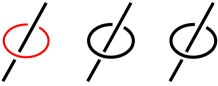
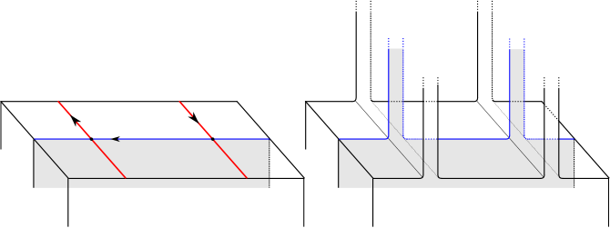
When it suits us, we are free to assume in proving Theorem 1.7 that is not right-veering, meaning that sends some arc in to the left at one of its endpoints, as shown in Figure 1 and made precise in [HKM07].
2pt
at 47 28 \pinlabel at 20 28 \pinlabel at 41 -3 \pinlabel at 65 57
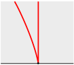
To see that we can make this assumption without loss of generality, note that one of or is not right-veering since otherwise and . (Indeed, if then we can take disjoint, properly embedded arcs which cut into a disk, and these arcs trace out embedded spheres in whose complement is minus balls, so gluing the spheres back in gives . Alternatively, the open book is a Murasugi sum of open books , each of which supports with its tight contact structure, and hence supports their connected sum.) If is right-veering then we can use the fact that knot Floer homology is invariant under reversing the orientation of and consider instead the knot with open book .
Recall that the knot Floer homology of is the homology of the associated graded object of a filtration
of the Heegaard Floer complex of induced by the knot. By careful inspection of a Heegaard diagram for adapted to the open book , Baldwin and Vela-Vick prove:
Lemma 1.12.
If the monodromy is not right-veering then there exist and such that generates and .
To see how Lemma 1.12 implies Theorem 1.11, let us assume that the monodromy is not right-veering. Given and as guaranteed by Lemma 1.12, it is then an easy exercise to see that and nonzero imply that the class
is nonzero. Theorem 1.11 then follows from the symmetry
Our strategy is to translate a version of this proof to the instanton Floer setting. Of course, it does not translate readily. For one thing, it makes use of Heegaard diagrams in an essential way. For another, it relies on a description of knot Floer homology as coming from a filtration of the Floer complex of the ambient manifold, for which there is no analogue in .
Our solution to these difficulties starts with a reformulation of Lemma 1.12 in terms of the minus version of knot Floer homology, which assigns to a knot a module over the polynomial ring . Specifically, we observe that Lemma 1.12 can be recast as follows:
Lemma 1.13.
If the monodromy is not right-veering then the generator of
is in the kernel of multiplication by .
Indeed, if we reverse the roles of the and basepoints in the above Heegaard diagram for , then we obtain a diagram for where the generators and lie in filtration gradings and , respectively. In , one records disks which cross the basepoint times with the coefficient , so the relation in from the original Heegaard diagram, which is certified by a holomorphic disk from to passing through once, becomes in after the basepoint swap; hence, in .
It may seem as though this reformulation of Lemma 1.12 makes translation even more difficult, as there is no analogue of whatsoever in the instanton Floer setting. Surprisingly, however, it is Lemma 1.13 that proves most amenable to translation.
Our approach is inspired by work of Etnyre, Vela-Vick, and Zarev, who provide in [EVVZ17] a more contact-geometric description of with its -module structure. As we show below, their work enables a proof of Lemma 1.13 in terms of sutured Floer homology groups, bypass attachment maps, and contact invariants. The value for us in proving Lemma 1.13 from this perspective is that while there is no analogue of in the instanton Floer setting, there are instanton Floer analogues of these groups, bypass maps, and contact invariants, due to Kronheimer and Mrowka [KM10b] and the authors [BS16b]. We are thus able to port key elements of this alternative proof of Lemma 1.13 to the instanton Floer setting and, with additional work, use these elements to prove Theorem 1.7. Below, we:
As the binding of the open book , the knot is naturally a transverse knot in . Moreover, we will show in Section 6 that has a Legendrian approximation with Thurston-Bennequin invariant
For each , let be the result of negatively Legendrian stabilizing the knot a total of times and then positively/negatively stabilizing the result one additional time. Note that each is also a Legendrian approximation of . Let
be the contact manifold with convex boundary and dividing set obtained by removing a standard neighborhood of from . These contact manifolds are related to one another via positive and negative bypass attachments. By work of Honda, Kazez, and Matić in [HKM08], these bypass attachments induce maps on sutured Floer homology,
for each , which satisfy
where refers to the Honda-Kazez-Matić contact invariant defined in [HKM09]. The main result of [EVVZ17] says that is isomorphic to the direct limit
of these sutured Floer homology groups and the negative bypass attachment maps. Moreover, under this identification, multiplication by is the map on this limit induced by the positive bypass attachment maps .
We now observe that Lemma 1.13 has a very natural interpretation and proof in this direct limit formulation. The first step is to identify the element of the direct limit which corresponds to the generator of . For this, recall that Vela-Vick proved in [VV11] that the transverse binding has nonzero invariant
where refers to the transverse knot invariant defined by Lisca, Ozsváth, Stipsicz, and Szabó in [LOSS09]. Moreover, this class lies in Alexander grading
| (3) |
according to [LOSS09]. So is the generator of
But Etnyre, Vela-Vick, and Zarev proved that corresponds to the element of the direct limit represented by the contact invariant
for any . It follows that corresponds to the element of the limit represented by
Lemma 1.13 therefore follows from the lemma below.
Lemma 1.14.
If the monodromy is not right-veering then
But this lemma follows immediately from the result below since the invariant vanishes for overtwisted contact manifolds.
Lemma 1.15.
If the monodromy is not right-veering then is overtwisted.
This concludes our alternative proof of Lemma 1.13, modulo the proof of Lemma 1.15 which we provide in Section 6. We now describe in detail our proof of Theorem 1.7, inspired by these ideas.
The instanton Floer analogues of and are the contact invariants
and bypass attachment maps
we defined in [BS16b]. Guided by the discussion above, our approach to proving Theorem 1.7 begins with the following analogue of Lemma 1.14.
Lemma 1.16.
If the monodromy is not right-veering then .
We note that Lemma 1.16 follows immediately from Lemma 1.15 since our contact invariant vanishes for overtwisted contact manifolds, just as the invariant does.
Unfortunately, Lemma 1.16 does not automatically imply Theorem 1.7 in the same way that Lemma 1.14 implies Theorem 1.11, as the latter implication ultimately makes use of structure that is unavailable in the instanton Floer setting. Indeed, proving Theorem 1.7 from the starting point of Lemma 1.16 requires some additional ideas, as explained below.
First, we recall that in [SV09], Stipsicz and Vértesi proved that the hat version of the Lisca, Ozsváth, Stipsicz, Szabó transverse invariant,
can be described as the invariant of the contact manifold obtained by attaching a certain bypass to the complement of a standard neighborhood of any Legendrian approximation of . In particular, the contact manifold resulting from these Stipsicz-Vértesi bypass attachments is independent of the Legendrian approximation, as shown in the proof of [SV09, Theorem 1.5]. Inspired by this, we define an element
where
is the map our work [BS16b] assigns to the Stipsicz-Vértesi bypass attachment. Since each is a Legendrian approximation of , the contact manifold obtained from these attachments, and hence , is independent of .
We prove that the invariant of the transverse binding lies in the top Alexander grading, just as in Heegaard Floer homology:
Theorem 1.17.
.
Moreover, we prove the following analogue of Vela-Vick’s result [VV11] that the transverse binding of an open book has nonzero Heegaard Floer invariant.
Theorem 1.18.
is nonzero.
Remark 1.20.
Our proof of Theorem 1.18 relies on formal properties of our contact invariants as well as the surgery exact triangle and adjunction inequality in instanton Floer homology. In fact, our argument can be ported directly to the Heegaard Floer setting to give a new proof of Vela-Vick’s theorem.
The task remains to put all of these pieces together to conclude Theorem 1.7. This involves proving a bypass exact triangle in sutured instanton homology analogous to Honda’s triangle in sutured Heegaard Floer homology. In Section 4 we prove the following.
Theorem 1.21.
Suppose is a 3-periodic sequence of sutures related by the moves in a bypass triangle as in Figure 2. Then there is an exact triangle
in which the maps are the corresponding bypass attachment maps.
2pt
\pinlabel at 24 117
\pinlabel at 149 118
\pinlabel at 97 37
\pinlabel at -3 145
\pinlabel at 173 144
\pinlabel at 85 -8
\endlabellist
For example, we show that the map fits into a bypass exact triangle of the form
| (4) |
as provided by Theorem 1.21, in which the map comes from attaching a Stipsicz-Vértesi bypass.
To prove Theorem 1.7, let us now assume that the monodromy is not right-veering. Then
by Lemma 1.16. Exactness of the triangle (4) then tells us that there is a class such that
The composition
| (5) |
therefore satisfies
which is nonzero by Theorem 1.18. It follows that the class is nonzero as well.
Although the map in (5) is not a priori homogeneous with respect to the Alexander grading, we prove that it shifts the grading by at most 1. On the other hand, this composition is trivial on the top summand
since by Theorems 1.17 and 1.18 this summand is generated by , and
by exactness of the triangle (4). This immediately implies the result below.
Theorem 1.22.
The component of in is nonzero.
Theorem 1.7 then follows from the symmetry
This completes our outline of the proof of Theorem 1.7. There are several challenges involved in making this outline rigorous. The most substantial and interesting of these has to do with the Alexander grading, as described below.
1.5. On the Alexander grading
Kronheimer and Mrowka define the Alexander grading on by embedding the knot complement in a particular closed -manifold. On the other hand, the argument outlined above relies on the contact invariants in we defined in [BS16b] and our naturality results from [BS15] (the latter tell us that different choices in the construction of yield groups that are canonically isomorphic, which is needed to talk sensibly about maps between groups). Both require that we use a much larger class of closures. Accordingly, one obstacle we had to overcome was showing that the Alexander grading can be defined in this broader setting in such a way that it agrees with the one Kronheimer and Mrowka defined (so that it still detects genus and fiberedness). We hope this contribution might prove useful for other purposes as well.
1.6. Organization
Section 2 provides the necessary background on instanton Floer homology, sutured instanton homology, and our contact invariants. We also prove several results in this section which do not appear elsewhere but are familiar to experts. In Section 3, we give a more robust definition of the Alexander grading associated with a properly embedded surface in a sutured manifold. In Section 4, we prove a bypass exact triangle in sutured instanton homology. In Section 5, we define invariants of Legendrian and transverse knots in and establish some of their basic properties. In Section 6, we prove Theorem 1.7 according to the outline above. As discussed, this theorem implies the other theorems stated above, including our main result that Khovanov homology detects the trefoil.
1.7. Acknowledgments
We thank Chris Scaduto and Shea Vela-Vick for helpful conversations, and the referees for many useful comments which improved the exposition. We also thank Etnyre, Vela-Vick, and Zarev for their beautiful article [EVVZ17] which inspired certain parts of our approach. Finally, we would like the acknowledge the debt this paper owes to the foundational work of Kronheimer and Mrowka.
2. Background
2.1. Instanton Floer homology
This section provides the necessary background on instanton Floer homology. Our discussion is borrowed from [KM10b], though we include proofs of some propositions and lemmas which are familiar to experts but do not appear explicitly elsewhere. Our description of the surgery exact triangle is taken from [Sca15]. All surfaces in this paper will be orientable.
Let be an admissible pair; that is, a closed, oriented 3-manifold and a closed, oriented 1-manifold intersecting some embedded surface transversally in an odd number of points. We associate the following data to this pair:
-
•
A Hermitian line bundle with Poincaré dual to ;
-
•
A bundle equipped with an isomorphism .
The instanton Floer homology is the Morse homology of the Chern-Simons functional on the space of connections on modulo determinant-1 gauge transformations, as in [Don02]. It is a -graded -module.
Notation 2.1.
Given disjoint oriented -manifolds we will use the shorthand
as it will make the notation cleaner in what follows.
For each even-dimensional class , there is an operator
defined by a cohomology class in ; these are introduced in [KM10b, §7.2] as a straightforward adaptation of a construction for closed 4-manifold invariants in [DK90], though they had already appeared in some form in [Muñ99]. These operators are additive in that
Moreover, any two such operators commute. Using work of Muñoz [Muñ99], Kronheimer and Mrowka prove the following in [KM10b, Corollary 7.2].
Theorem 2.2.
Suppose is a closed surface in of positive genus with odd. Then the simultaneous eigenvalues of the operators and on belong to a subset of the pairs
for and , where .
With this, they make the following definition.
Definition 2.3.
The commutativity of these operators implies that for any closed surface the operator acts on . Moreover, Kronheimer and Mrowka obtain the following bounds on the spectrum of this operator without the assumption that is odd [KM10b, Proposition 7.5].
Proposition 2.4.
For any closed surface of positive genus, the eigenvalues of
belong to the set of even integers between and .
We are interested in studying the eigenspace decompositions of operators of the form , which may not be diagonalizable. In this section, we will use eigenspace in proofs to mean generalized eigenspace, but in the statements of results we will always say “generalized eigenspace” so that they can be understood unambiguously later.
Lemma 2.5.
If then the generalized -eigenspace of acting on is isomorphic to its generalized -eigenspace for each .
Proof.
Suppose . Then the -eigenspace of acting on is the simultaneous -eigenspace of the operators on . Recall that is a -graded group. We may thus write an element of this group as , where is in grading mod 8. It then follows immediately from the fact that and are degree 2 operators and is a degree 4 operator that the map which sends
defines an isomorphism from the -eigenspace of to the -eigenspace of these operators. ∎
Suppose and are admissible pairs. A cobordism from the first pair to the second induces a map
which depends up to sign only on the homology class and the isomorphism class of , where two such pairs are isomorphic if they are diffeomorphic by a map which intertwines the boundary identifications (the surface specifies a bundle over restricting to the bundles on the boundary specified by and ). Moreover, if and are homologous in then
| (6) |
which implies the following.
Lemma 2.6.
Suppose is in the generalized -eigenspace of . Then is in the generalized -eigenspace of .
Proof.
Since is in the -eigenspace of , there exists an integer such that
The relation (6) then implies that
which confirms that is in the -eigenspace of . ∎
A similar result holds if is the disjoint union of two admissible pairs
In this case, induces a map
Moreover, if
is homologous in to then
| (7) |
which implies the following analogue of Lemma 2.6.
Lemma 2.7.
Suppose is in the generalized -eigenspace of and is in the generalized -eigenspace of . Then is in the generalized -eigenspace of .
Proof.
Under the hypotheses of the lemma, there exists an integer such that
It follows easily from the relation (7) that
Each term in this sum vanishes since either or , which confirms that lies in the -eigenspace of . ∎
Lemmas 2.6 and 2.7 will be used repeatedly in Section 3. They are also used to prove the next proposition and its corollary, which will in turn be important in the proof of Theorem 1.7 in Section 6. In particular, Proposition 2.8 will be used to constrain the Alexander grading shift of the map described in Section 1.4.
Suppose for the proposition below that is a cobordism from to and that and are closed surfaces of the same positive genus which are homologous in with and odd. Then Lemma 2.6 implies that restricts to a map
Proposition 2.8.
Suppose and are closed surfaces and is a closed surface of genus and self-intersection such that
in . If belongs to the generalized -eigenspace of , then we can write
where each lies in the generalized -eigenspace of the action of on .
Proof.
First, suppose is odd. Consider the cobordism
obtained from by removing a tubular neighborhood of . We may assume that intersects a fiber transversely in an odd number of points. Then for we have
where is the cobordism map
and is the relative invariant of the -manifold . From the discussion above, we can write
where is in the -eigenspace of the operator on . Recall that an element lies in the -eigenspace of on by definition. Since a point in either or is homologous to a point in , Lemma 2.7 implies that lies in both the - and -eigenspaces of on . Thus,
We therefore have that
From the discussion above, we can write as a sum
where each is in the -eigenspace of the operator on
Suppose belongs to the -eigenspace of the operator as in the proposition. It then follows from Lemma 2.7 that
lies in the -eigenspace of for each . We may therefore write
where
is in the -eigenspace of .
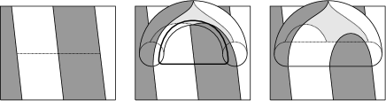
Now suppose is even. We claim that there is a surface homologous to of genus . Let be a tubular neighborhood of in . Let be a parallel copy of in . We cut open along a non-separating curve , cut open along a parallel curve , and glue these cut open surfaces together in a way that is consistent with their orientations and results in a connected surface of genus . Figure 3 shows how we modify in to obtain , where is an annular neighborhood of in .
2pt \pinlabel at 18 54 \pinlabel at 20 84

By tubing to a copy of , we obtain a closed surface homologous to of genus , where . This surface has odd and self-intersection , and we have the relation
in . Now suppose that belongs to the -eigenspace of . Then belongs to the -eigenspace of . The argument in the previous case tells us that we can write
where each lies in the -eigenspace of the action of on . Then
and the right side is again zero for large enough, meaning that is in the -eigenspace of . Since
we have that
Since the eigenvalues of must also be even integers, we see that the minimum eigenvalue of showing up in the expansion of into eigenvectors of is . Applying the same argument but for a surface homologous to of genus and satisfying
shows that the maximum eigenvalue of showing up in the expansion of is . This proves the result. ∎
For the corollary below, suppose are such that is defined.
Corollary 2.9.
Suppose are closed surfaces of the same genus and is a closed surface of genus such that
in . If belongs to the generalized -eigenspace of , then we can write
where each lies in the generalized -eigenspace of the action of on .
Proof.
Simply apply Proposition 2.8 to the product cobordism from to itself. ∎
We will make repeated use of the surgery exact triangle in instanton Floer homology. This triangle goes back to Floer but appears in the form below in work of Scaduto [Sca15].
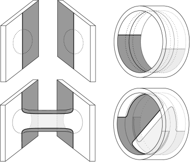
Suppose is a framed knot in . Let be an oriented -manifold in which is disjoint from . Let denote the result of -surgery on , and let be the induced -manifold in , for . There is then a sequence of -handle cobordisms
| (8) |
which induce homomorphisms on instanton Floer homology that fit into an exact triangle as follows.
Theorem 2.10.
There is an exact triangle
as long as , and are all admissible pairs. Here each of , , and is a properly embedded surface in , , or bounded by the indicated 1-manifolds at either end: is the union of a product cylinder from to and a closed surface, and and are each the union of the analogous product cylinder with a disk bounded by in the corresponding 2-handle.
2pt \pinlabel at 25 100 \pinlabel at 62.5 51 \pinlabel at 96.5 51 \pinlabel at 26.5 51 \pinlabel at 26.5 17.5 \pinlabel at 61.5 17.5 \pinlabel at 96.5 17.5 \pinlabel at 59 100 \pinlabel at 94 100 \pinlabel at 25 66.5 \pinlabel at 59.5 66.5 \pinlabel at 93.5 66.5 \pinlabel at 25 33 \pinlabel at 59.5 33 \pinlabel at 93.5 33
at 14 1.5 \pinlabel at 49 1 \pinlabel at 83 1
Since each manifold in the surgery exact triangle is obtained from the preceding one via integer surgery, we can in fact produce three different surgery exact triangles involving the same 3-manifolds and 4-dimensional cobordisms. This is illustrated in Figure 4, where in each row we use a different pair of 3-manifold and framed knot to construct an exact triangle; in the first row, we use to recover Theorem 2.10, while the other two exact triangles correspond to surgeries on and . The only differences between these three triangles are the 1-manifolds used to define the instanton Floer groups and the 2-dimensional cobordisms between those 1-manifolds.
2.2. Sutured instanton homology
This section provides the necesary background on sutured instanton homology. Our discussion is adapted from [BS15, BS16b], though the basic construction of is of course due to Kronheimer and Mrowka [KM10b].
2.2.1. Closures of sutured manifolds
We first recall the following definition.
Definition 2.11.
A balanced sutured manifold is a compact, oriented 3-manifold together with an oriented multicurve whose components are called sutures. Letting
oriented as a subsurface of , it is required that:
-
•
neither nor has closed components,
-
•
with , and
-
•
.
The following examples will be important for us.
Example 2.12.
Suppose is a compact, connected, oriented surface with nonempty boundary. The pair
is called a product sutured manifold.
Example 2.13.
Given a knot in a closed, oriented -manifold , let
where is a tubular neighborhood of and and are oppositely oriented meridians.
Definition 2.14.
An auxiliary surface for is a compact, connected, oriented surface with the same number of boundary components as components of .
Suppose is an auxiliary surface for , that is a tubular neighborhood of , and that
is an orientation-reversing diffeomorphism.
Definition 2.15.
We form a preclosure of
by gluing to according to .
This preclosure has two diffeomorphic boundary components,
where
Let and choose an orientation-reversing diffeomorphism
which fixes a point . We form a closed -manifold
by gluing to according to the maps
and we let and be the natural inclusions.
Let be the curve formed as the union of the arcs
Choose a nonseparating curve ; we note that this requires . For convenience, we will also use to denote the distinguished surface and to denote the curve .
Definition 2.16.
We refer to the tuple as a closure of .222In [BS16b], we called such a tuple a marked odd closure.
The genus refers to the genus of .
Remark 2.17.
Suppose is a closure of . Then the tuple
is a closure of
2.2.2. Sutured instanton homology
Following Kronheimer and Mrowka [KM10b], we make the definition below.
Definition 2.18.
Given a closure of , the sutured instanton homology333In [BS15], we called this the twisted sutured instanton homology and denoted it by instead. of is the -module
Kronheimer and Mrowka proved that, up to isomorphism, is an invariant of . (In fact, they took to be their invariant, but proved it isomorphic to via excision.) In [BS15], we constructed for any two closures of of genus at least two a canonical isomorphism
which is well-defined up to multiplication in . (See the proof of Theorem 3.5 for details of the construction.) In particular, these isomorphisms satisfy, up to multiplication in ,
for any triple of such closures. The groups and isomorphisms ranging over closures of of genus at least two thus define what we called a projectively transitive system of -modules in [BS15].
Definition 2.19.
The sutured instanton homology of is the projectively transitive system of -modules defined by the groups and canonical isomorphisms above.
Remark 2.20.
The isomorphisms are defined using -handle and excision cobordisms. We will provide more details in Section 3, where we show that these isomorphisms respect the Alexander gradings associated to certain properly embedded surfaces in .
Remark 2.21.
We emphasize that if either or has genus one, then there is still an isomorphism , though it may not be canonical. We will show in Theorem 3.5 that even these non-canonical isomorphisms respect the Alexander gradings, which will be necessary to relate our Alexander grading to one defined by Kronheimer and Mrowka (see Remarks 3.10 and 3.11).
The following result of Kronheimer and Mrowka [KM10b, Proposition 7.8] will be important for us. We sketch their proof below so that we can refer to this construction later.
Proposition 2.22.
Suppose is a product sutured manifold as in Example 2.12. Then
Proof.
Let be an auxiliary surface for . Form a preclosure by gluing to according to a map
of the form for some diffeomorphism . This preclosure is then a product
To form a closure, we let and glue to by maps
as usual, where fixes a point on . We then define and as described earlier to obtain a closure , where
is the surface bundle over the circle with fiber and monodromy . We then have that
by [KM10b, Proposition 7.8] in the case , and more generally by excision [KM10b, Theorem 7.7] exactly as in the proof of [KM10b, Lemma 4.7]. ∎
As mentioned in the introduction, Kronheimer and Mrowka define in [KM10b, Section 7.6] the instanton Floer homology of a knot as follows.
Definition 2.23.
Suppose is a knot in a closed, oriented -manifold . The instanton knot Floer homology of is given by
where is the knot complement with two meridional sutures as in Example 2.13.
2.2.3. Contact handle attachments and surgery
In [BS16b], we defined maps on associated to contact handle attachments and surgeries, which we will review below; see Figure 5 for illustrations of such handle attachments. These contact handle attachments can be viewed purely as operations on sutured manifolds, and this is the perspective we take in this subsection. However, we will first motivate the name by summarizing the contact geometric origin of this construction, which we will return to in Section 2.3.
A collection of sutures specifies an -invariant contact structure in a collar neighborhood of , for which is convex with dividing set ; see [Gir91] for details on convex surfaces. We can then naturally glue other contact manifolds with convex boundaries to by orientation-reversing diffeomorphisms which identify the dividing sets. For example, if we view as the unit disk in the plane and let , then has a tight contact form which makes the boundary convex. Its dividing set is disconnected, consisting of the four arcs
lying on and respectively. Attaching a contact 1-handle means gluing this to along by a map taking dividing curves to sutures, whereas a contact 2-handle is instead glued along . In either case we get a manifold with corners, and when we smooth them out, Honda’s “edge-rounding” procedure [Hon00, Lemma 3.11] tells us how to connect the various sutures/dividing arcs on the boundary, exactly as shown in Figure 5.
From here on we will suppress the inclusion maps and from the notation specifying a closure , since any time we want to use to construct some new closure there will be a natural, essentially unique way to define the corresponding and .
2pt \pinlabel at 300 277
First, we consider contact -handle attachments.
Suppose is obtained from by attaching a contact -handle. Then one can show that any closure of the first also naturally specifies a closure of the second (the only difference between these closures are the embeddings ). We therefore define the -handle attachment map
to be the identity map on instanton Floer homology. For closures of genus at least two, these maps commute with the canonical isomorphisms described above and thus define a map
as in [BS16b, Section 3.2].
Next, we consider contact -handle attachments.
Suppose is obtained from by attaching a contact -handle along a curve . Let be a closure of . We proved in [BS16b, Section 3.3] that -framed surgery on naturally yields a closure of , where is the surgered manifold. Let
be the cobordism obtained from by attaching a -handle along , and let be the cylinder
The fact that is disjoint from means that and are isotopic in . Since these surfaces have the same genus, Lemma 2.6 implies that the induced map
restricts to a map
For closures of genus at least two, these maps commute with the canonical isomorphisms and therefore define a map
as shown in [BS16b, Section 3.3].
Finally, we consider surgeries.
Suppose is obtained from via -surgery on a framed knot . A closure of naturally gives rise to a closure of , where is the surgered manifold as in the -handle attachment case. The -handle cobordism corresponding to this surgery induces a map
| (9) |
as in the previous case. We showed in [BS16b, Section 3.3] that for closures of genus at least two, these maps commute with the canonical isomorphisms and thus give rise to a map
Remark 2.24.
We have asserted that all of the handle-attaching and surgery maps commute with the canonical isomorphisms when the closures and have genus at least two, but this restriction can be weakened: if either closure has genus one, then these maps still commute with the non-canonical isomorphisms mentioned in Remark 2.21.
2.3. The contact invariant
We assume some familiarity with contact structures and open books; see Etnyre [Etn03] or Geiges [Gei08] for a general introduction, Etnyre [Etn06] for material on open books, and Massot [Mas14] for convex surfaces. One of the key things we will take from convex surface theory is Giroux flexibility [Gir91], which essentially says that given a surface and multicurve bounding a subsurface , there is a unique (up to isotopy) vertically invariant contact structure on such that is convex with dividing set . In particular, this allows us to glue contact structures along convex surfaces with the same dividing sets.
The background material on partial open books is introduced in large part to establish common notation. In what follows, we write to refer to a contact manifold with nonempty convex boundary and dividing set ; we call such a triple a sutured contact manifold.
Definition 2.25.
A partial open book is a triple , where:
-
•
is a connected, oriented surface with nonempty boundary,
-
•
is a subsurface of formed as the union of a neighborhood of with -handles in , and
-
•
is an embedding which restricts to the identity on .
Definition 2.26.
A basis for a partial open book is a collection
of disjoint, properly embedded arcs in such that deformation retracts onto ; essentially, the basis arcs in specify the cores of -handles used to form .
A partial open book specifies a sutured contact manifold as follows.
Suppose is a partial open book with basis . Let be the unique tight contact structure on the handlebody
For , let be the curve on given by
| (10) |
Definition 2.27.
We define to be the sutured contact manifold obtained from by attaching contact -handles along the curves above.
Remark 2.28.
Up to a canonical isotopy class of contactomorphisms, does not depend on the choice of basis . It does depend on , however, via the -handles attached along the , which can be understood as gluing each arc to its image .
Definition 2.29.
A partial open book decomposition of consists of a partial open book together with a contactomorphism
for some basis of .
Remark 2.30.
We will generally conflate partial open book decompositions with partial open books. Given a partial open book decomposition as above, we will simply think of as being equal to . In particular, we will view as obtained from by attaching contact -handles along the curves in (10).
Half of the relative Giroux correspondence, proven in [HKM09], states the following.
Theorem 2.31.
Every admits a partial open book decomposition.
Example 2.32.
Given an open book decomposition of a closed contact manifold , the triple
is a partial open book decomposition for the complement of a Darboux ball in .
Example 2.33.
Given an open book decomposition of a closed contact manifold with a Legendrian knot realized on the page , the triple
is a partial open book decomposition for the complement of a standard neighborhood of .
To define the contact invariant of , we choose a partial open book decomposition of . Let be a basis for and let
be the corresponding curves as in (10). Let
be the composition of the maps associated to contact -handle attachments along the curves , as described in Section 2.2.3. Recall from Proposition 2.22 that
and let be a generator of this group. The following is from [BS16b, Definition 4.2].
Definition 2.34.
We define the contact class to be
As the notation suggests, this class does not depend on the partial open book decomposition of . Indeed, we proved the following in [BS16b, Theorem 4.3].
Theorem 2.35.
is an invariant of the sutured contact manifold .
We will often think about the contact class in terms of closures. For that point of view, let be a closure of with
as in the proof of Proposition 2.22. As mentioned in the definition of the contact -handle attachment maps, performing -framed surgery on the curves
naturally yields a closure of . We then define
where
is the map associated to the corresponding -handle cobordism , is the usual cylindrical cobordism, and is a generator of
In particular, this class is well-defined up to multiplication in . Our invariance result is then the statement that the classes defined in this manner, for any partial open book decompositions and closures of genus at least two, are related by the canonical isomorphisms between the groups assigned to different closures.
Remark 2.36.
For convenience of notation, we will often use the shorthand and to denote the classes and , respectively.
Below are some important properties of the contact class, all proven in [BS16b, Section 4.2]. In brief, the contact class vanishes for overtwisted contact manifolds and behaves naturally with respect to contact handle attachment and contact -surgery on Legendrian knots. We view both contact 1-handles and contact 2-handles as having the unique -invariant contact structure on whose dividing set on is a properly embedded arc, as described at the beginning of Section 2.2.3.
Theorem 2.37.
If is overtwisted then .
Theorem 2.38.
Suppose is the result of attaching a contact -handle to for or . Then the associated map
defined in Section 2.2.3 sends to .
Theorem 2.39.
Suppose is a Legendrian knot in and that is the result of contact -surgery on . Then the associated map
defined in Section 2.2.3 sends to .
For the sake of later applications, we now observe that the map fits into a surgery exact triangle, where the third term involves the Floer homology of the sutured manifold obtained by -surgery on . Suppose is obtained from via -surgery on a framed knot . Let be a closure of , and let
be the tuples obtained from by performing - and -surgery on . These are naturally closures of the sutured manifolds
Note that and are obtained from surgeries on ,
By Theorem 2.10 (and Lemma 2.6), there is an exact triangle
| (11) |
Here, is the curve in corresponding to the meridian of , as in Figure 6; and is the product in , which was called in (9), so we have .
Strictly speaking, this triangle is one of the variations described after Theorem 2.10, corresponding to the second row of Figure 4; again, the 3-manifolds and cobordisms between them are the same, but the 1-manifolds and cobordisms between them are different. This particular exact triangle corresponds to surgery on , with its usual framing inherited from , since - and -surgeries on produce and .
2pt \pinlabel at 26.5 16.5 \pinlabel at 61 16.5 \pinlabel at 95 16.5
at 60.5 34 \pinlabel at 26 34 \pinlabel at 94.5 34
at 12 1 \pinlabel at 46 1 \pinlabel at 81 1
3. The Alexander grading
In [KM10b, Section 7.6], Kronheimer and Mrowka explain how a Seifert surface for a knot gives rise to an “Alexander grading” on the instanton knot Floer homology defined in Definition 2.23; the name indicates that together with this grading categorifies the Alexander polynomial of . In their construction, they use a genus one closure of formed with an annular auxiliary surface. In this section, we describe how more generally a properly embedded surface in any sutured manifold which intersects the sutures twice gives rise to a grading on , which we also call an Alexander grading, using closures of any genus. In particular, we prove that this grading is preserved by the canonical isomorphisms relating the groups assigned to different closures.
Before beginning the discussion in earnest, we recall why this is necessary. In Section 5 we will define an invariant which associates to a transverse knot an element
In Section 6 we will prove that if is the connected binding of an open book supporting , with fiber surface , then generates the top Alexander grading . Its grading is determined in Theorem 1.17, which we prove by computing for a certain contact structure the Alexander grading of our contact invariant
where the sutures are not meridional, and then showing that is the image of this invariant under a map which preserves this grading. This argument therefore requires a notion of grading for more general choices of sutures. In fact, even in the case of , we need a more general construction because cannot be defined directly using Kronheimer and Mrowka’s preferred genus one closures.
Suppose is a balanced sutured manifold and is a properly embedded, oriented surface in with one boundary component such that the closed curve intersects transversely in two points, and , and let
as shown in Figure 7. To define the Alexander grading on associated with , we first cap off in a closure of .
2pt \pinlabel at 94 87 \pinlabel at 204 87 \pinlabel at 68 99 \pinlabel at 230 99 \pinlabel at 148 98 \pinlabel at 55 59 \pinlabel at 332 59
at 342 99 \pinlabel at 427 98 \pinlabel at 358 143 \pinlabel at 387 143
at 467 143 \pinlabel at 496 143
Let be an auxiliary surface with an identification
we note that and need not be connected. Let be an annular neighborhood of such that intersects in the arcs
and let
be the diffeomorphism . Let be the preclosure obtained by gluing to according to . Let be a nonseparating, properly embedded arc in with endpoints at and . Let be the properly embedded surface in obtained as the union of with the 1-handle , as shown in Figure 7. The boundary of consists of the two circles
where . The fact that is nonseparating in implies that the circles are nonseparating in . In forming a closure, we can therefore choose a diffeomorphism
which identifies with . Let and let
be the closed manifold formed according to in the manner described in Section 2.2, immediately after Definition 2.15. We define
in the usual way, for some fixed by , and choose for a curve which intersects in one point. (This last condition will be useful at the beginning of the proof of Theorem 3.5.)
Definition 3.1.
We say that a closure defined as above is adapted to .
By way of comparison, Kronheimer and Mrowka insist in [KM10b] that be the complement of a null-homologous knot in a closed manifold , with a pair of oppositely-oriented meridians. They then work with a specific genus-one closure (denoted in [KM10b, Definition 5.4]) which is adapted to any Seifert surface for .
Let
be the closed surface in obtained as the union of with the annulus . Note that is obtained from by capping off its boundary with a punctured torus, so that
We use to define an Alexander grading on , generalizing the construction of [KM10b, Section 7.6], as follows.
Definition 3.2.
Given a closure of adapted to , the sutured instanton homology of in Alexander grading relative to is the generalized -eigenspace of the operator
We denote this generalized eigenspace by .
Remark 3.3.
As the notation above suggests, the Alexander grading on relative to depends only on the class
as this class determines the homology class of , and the operator depends only on .
Lemma 3.4.
The group is trivial for . Thus,
Proof.
This follows immediately from Proposition 2.4, which implies that the eigenvalues of on belong to the set of even integers from to . ∎
We next prove that this construction gives a well-defined Alexander grading on .
Theorem 3.5.
Suppose and are closures of adapted to . For each , we have
Moreover, when and have genus at least two, the canonical isomorphism restricts to an isomorphism
for each .
Proof.
We will proceed in two steps: first we consider closures of the same genus, and then we see what happens when we increase the genus by one. In the first case, the isomorphism is built out of cobordism maps induced by Dehn surgeries, and these surgeries avoid the closed surfaces and built from whose eigenspaces define the Alexander grading, so the grading passes through unchanged. In the second case, we choose a convenient closure whose auxiliary portion can be cut open to “insert” extra genus, leading to a closure of genus . Then is realized by a more complicated “excision” cobordism, and we will have to work a bit harder to relate the homology classes (and hence eigenspaces) of and on either end of this cobordism.
To begin, we let
be closures of adapted to . Let us suppose first that . Since the curves and are essential in and intersect in one point, we can find a diffeomorphism
| (12) |
which identifies with the corresponding . We can also ensure that this map sends the point defining to the corresponding point defining .
Note that for genus closures, there is a unique isotopy class of such diffeomorphisms since the complements
are disks in this case. Thus, we automatically have
when . More generally, the diffeomorphism in (12) allows us to view and as formed from the same preclosure , according to different diffeomorphisms
where is a diffeomorphism of fixing . We may factor as a composition of positive and negative Dehn twists around curves
disjoint from . This then allows us to view as obtained from via -surgeries on copies
of the .
Suppose first that only positive Dehn twists appear in the factorization of . Let be the associated cobordism from to , obtained from by attaching -framed -handles along the in , with . Since and are isotopic in and
Lemma 2.6 implies that the induced map
restricts to a map
| (13) |
The map in (13) defines the canonical isomorphism when both closures have genus at least 2 [BS15, Definition 9.10]. Since the are disjoint from , the surgery curves are disjoint from the annulus which caps off the surface to form . The capped off surfaces and are therefore isotopic in . Lemma 2.6 then implies that restricts to an isomorphism
for each , as claimed.
If both positive and negative Dehn twists appear in the factorization of then the isomorphism relating and is defined as the composition of a map as in (13) with the inverse of such a map, so the same argument applies.
Next, suppose is a closure of adapted to as in the beginning of this section, and let us borrow the notation used there. We will construct a closure adapted to with
and show that the isomorphism relating and preserves Alexander gradings.
To start, let be a closed curve dual to the arcs and (we can choose so that these arcs are parallel). Let us assume that the map
used to form identifies the curves
Let be a closed genus 2 surface containing parallel curves and and a curve dual to both. Let be the surface obtained by cutting and open along and and gluing these cut-open surfaces together according to a homeomorphism of their boundaries which identifies and with and , respectively, as shown in Figure 8.
2pt \pinlabel at 25 23 \pinlabel at 345 22
at 60 24 \pinlabel at 177 23 \pinlabel at 382 23 \pinlabel at 60 97 \pinlabel at 28 97 \pinlabel at 92 65 \pinlabel at 25 53 \pinlabel at 179 97 \pinlabel at 142 65 \pinlabel at 178 52 \pinlabel at 347 96 \pinlabel at 382 98 \pinlabel at 347 54
The union is then a nonseparating, properly embedded arc in . Let
be the closure of adapted to formed using the auxiliary surface and a diffeomorphism which restricts to
and to
In particular, identifies the two circles
so that caps off to a closed surface in in the usual manner.
Note that is obtained by cutting and open along the tori
and , respectively, and regluing. From this point of view, the capped off surface is obtained by cutting and the torus open along essential curves and regluing. There is a standard excision-type cobordism
associated to this cutting and regluing, as described in [KM10b, Section 3] and [BS15, Section 9.3.2], and a corresponding map
Kronheimer and Mrowka prove in [KM10b, Proposition 7.9] that the generalized -eigenspace of the operator acting on is one-dimensional. Let be a generator of this eigenspace. Then, since the disjoint union of surfaces
is homologous in to , and
Lemma 2.7 implies that defines a map
| (14) |
The map in (14) is an isomorphism [KM10b, Section 3]. (Roughly, we can glue to an excision-type cobordism in the other direction, and the result can be turned into a product cobordism by replacing an embedded with two copies of ; this only changes the induced map on the top eigenspace by a scalar factor, so it must have been an isomorphism.) Moreover, it agrees with the canonical isomorphism defined in [BS15] when .
Since intersects the torus in a single point, Theorem 2.2 says that the only eigenvalue of acting on is . It follows that the generalized -eigenspace of on is simply the group we denote by We therefore have that
Note that the only eigenvalue of acting on is by Proposition 2.4 since is a torus. In particular, is in the generalized -eigenspace of this operator . Then, since the disjoint union of surfaces
is homologous in to , Lemma 2.7 implies that the map restricts to an isomorphism
for each .
Finally, for any two closures and of adapted to , we define the isomorphism (the canonical isomorphism if both closures have genus at least 2)
to be a composition of isomorphisms defined as above. This completes the proof. ∎
Given Theorem 3.5, we make the following definition for a surface in as above.
Definition 3.6.
The sutured instanton homology of in Alexander grading relative to is the projectively transitive system of -modules
consisting of the groups for , together with the canonical isomorphisms between them from Theorem 3.5.
Remark 3.7.
Remark 3.8.
If admits a genus one closure then the Alexander grading on with respect to is symmetric by Lemma 2.5. That is,
for each .
Following [KM10b, Section 7.6], we make the definition below.
Definition 3.9.
Given a knot in a closed, oriented -manifold with Seifert surface , the instanton knot Floer homology of in Alexander grading relative to is
When the relative homology class of is unambiguous we will omit it from the notation.
Remark 3.10.
Remark 3.11.
Since the knot complement admits a genus one closure, the Alexander grading on relative to is symmetric by Remark 3.8. That is,
for each .
Kronheimer and Mrowka proved the following three results. The first follows from [KM10b, Theorem 7.18] and the discussion at the end of [KM10b, Section 7.6]; the second is [KM10b, Proposition 7.16]; and the third is [KM10a, Proposition 4.1]. As explained in the introduction, all three are important in our proof of Theorem 1.6.
Theorem 3.12.
If is fibered with fiber then .
Theorem 3.13.
For , .
Theorem 3.14.
For , if and only if is fibered.
4. The bypass exact triangle
In this section, we prove the bypass exact triangle, stated in the introduction as Theorem 1.21. Our proof is very similar to the proof we gave in [BS16a, Section 5] for sutured monopole homology, and we will rely on the topological ideas developed there. We must be a bit careful in the instanton Floer setting, however, with the bundles involved in the exact triangle.
Suppose is a balanced sutured manifold and is an arc which intersects transversally in three points, including both endpoints of . A bypass move along replaces with a new set of sutures which differ from in a neighborhood of , as shown in Figure 9.
2pt \pinlabel at 22 28
As background, bypasses were introduced by Honda [Hon00, §3.4]. The rough idea, also present in [Gir00], is that a contact structure on a thickened surface can be described in terms of some discrete data, namely the dividing curves on and finitely many times in at which the dividing curves on change. These changes are modeled by taking to be the boundary of a neighborhood of , where the bypass is a certain half-disk with Legendrian boundary, attached to along an arc as shown in Figure 9, and then the change in dividing curves from to is precisely a bypass move. They have been widely applied to classify tight contact structures on many 3-manifolds, as well as Legendrian representatives of various smooth knot types in ; the original use in [Hon00] was to classify tight contact structures on lens spaces.
A bypass move can be achieved by attaching a contact -handle along disks in centered at the endpoints of and then attaching a contact -handle along the union of with an arc on the boundary of this -handle, as shown in Figure 10. We refer to this sequence of handle attachments as a bypass attachment along , following [Hon00, Ozb11]. A bypass attachment along therefore gives rise to a morphism
which is the composition of the corresponding contact - and -handle attachment maps defined in Section 2.2.2. Theorem 2.38 implies the following.
2pt \pinlabel at 51 56 \pinlabel at 242 36 \endlabellist
Proposition 4.1.
Suppose is obtained from by attaching a bypass along . Then the induced map sends to .
Figure 11 shows a sequence of bypass moves, performed in some fixed neighborhood in , resulting in a 3-periodic sequence of sutures on . Such a sequence is called a bypass triangle. Unpublished work of Honda shows that a bypass triangle gives rise to a bypass exact triangle in sutured Heegaard Floer homology. We proved a similar result in the monopole Floer setting in [BS16a, Theorem 5.2]. Here, we prove the analogue for sutured instanton homology, stated below.
2pt
\pinlabel at 24 117
\pinlabel at 149 118
\pinlabel at 97 37
\pinlabel at -3 145
\pinlabel at 173 144
\pinlabel at 85 -8
\endlabellist
Theorem 1.21.
Suppose is a 3-periodic sequence of sutures resulting from successive bypass moves along arcs as in Figure 11. Then there is an exact triangle
in which are the corresponding bypass attachment maps.
Proof.
The main idea behind the proof is that there are closures of these three sutured manifolds which are related as in the surgery exact triangle of Theorem 2.10. This was first shown in the proof of [BS16a, Theorem 5.2] by an argument we review below. Unlike in the monopole Floer case, though, it is not obvious that the cobordism maps in the surgery exact triangle relating the instanton Floer groups of these closures are the same as those which induce the bypass attachment maps on , as the bundles on these cobordisms are different in the two cases. However, we show that one can choose closures so that any two of the three maps agree with those that induce the bypass attachment maps. This allows us to prove exactness of the triangle in Theorem 1.21 at each group, one group at a time.
Note that by enlarging our local picture slightly, we can think of the arcs as being arranged as in Figure 12 with respect to . We may therefore view
as being obtained from by attaching bypasses along the arcs
respectively. As described above, attaching a bypass along amounts to attaching a contact -handle along disks centered at the endpoints of and then attaching a contact -handle along a curve which extends over the handle, as in Figure 12. Let be the sutured manifold obtained by attaching all three to , as in Figure 12. For , let be the result of attaching a contact -handle to along . Then
2pt
\pinlabel at 61 79
\pinlabel at 106 181
\pinlabel at 151 282
\pinlabel at 769 71
\pinlabel at 815 173
\pinlabel at 861 273
\endlabellist
Recall from Section 2.2.2 that contact -handle attachment has little effect on the level of closures. Specifically, a closure of a sutured manifold after a -handle attachment can also be viewed naturally as a closure of the sutured manifold before the -handle attachment, and the corresponding -handle attachment morphism is simply the identity map. We therefore have canonical identifications
for , where the subscript of is taken mod . In particular, is canonically identified with . Therefore, to prove Theorem 1.21, it suffices to prove that there is an exact triangle
| (15) |
where is the map associated to contact -handle attachment along .
Recall that on the level of closures, contact -handle attachment corresponds to surgery. Specifically, if is a closure of , then there is a closure of of the form , where is the result of -framed surgery on . To see this, we write and consider the effect of the surgery operation on each of and separately. Since sits on the boundaries of both and , removing a small neighborhood carves a piece out of each without changing their topology. After doing so, the intersection is now an annulus fibered by -framed push-offs of , and the surgery fills each of them with a disk, which amounts to gluing a 2-handle to along . The same happens on the auxiliary part of the closure, where gluing in the family of disks now effectively adds a handle to the auxiliary surface that was used to construct , filling in the arcs that the 2-handle operation removes from , so that this surgery leads to a closure of without having to change the surface .
Having said this, the map is now induced by the -handle cobordism map
corresponding to this surgery, where is the usual cylindrical cobordism
In order to prove the exactness of the triangle (15) at , say, it therefore suffices to prove exactness of the sequence
| (16) |
Our approach is to find a closure of such that the surgeries relating the above are exactly the sort one encounters in the surgery exact triangle of Theorem 2.10, as depicted in Figure 4. Fortunately, the proof of [BS16a, Theorem 5.2] shows that for any closure ,
-
•
is the cobordism associated to -surgery on some ,
-
•
is the cobordism associated to -surgery on a meridian of ,
-
•
is the cobordism associated to -surgery on a meridian of ,
as desired. Theorem 2.10 then says that there is an exact sequence of the form
| (17) |
Note that this sequence (17) is subtly different from that in (16). For one thing, the Floer group on the left is defined using the -manifold rather than On the other hand, this group depends, up to isomorphism, only on the homology class of this -manifold, and we can find a closure such that is null-homologous in . Indeed, the construction in the beginning of Section 3, and illustrated in Figure 7, shows that for any curve (like ) in the boundary of a sutured manifold which intersects the sutures twice, we can find a closure in which this curve bounds a once-punctured torus such that the framing on the curve induced by this surface agrees with the framing induced by the boundary. Let be such a closure. Then (17) becomes the exact sequence
| (18) |
where is the cobordism given as the composition of the once-punctured torus viewed as a cobordism from to with . To deduce (16) from (18), it suffices to show that
| (19) |
Recall that these maps depend only on the relative homology classes of the various -dimensional cobordisms involved. Since we have chosen a closure in which is nullhomologous in and is obtained via -surgery on with respect to the framing induced by the once-punctured torus providing the nullhomology, we have that
The long exact sequence of the pair shows in this case that a relative homology class in is determined by its boundary. Since and have the same boundary, they represent the same class, which then implies the first equality in (19); likewise, for the second equality. This proves that the triangle in (15) is exact at . Identical arguments show that it is exact at the other groups, completing the proof of Theorem 1.21. ∎
5. Invariants of Legendrian and transverse knots
In this section, we define invariants of Legendrian and transverse knots in instanton knot Floer homology. As described in the introduction, our construction is motivated by Stipsicz and Vértesi’s interpretation [SV09] of the Legendrian and transverse knot invariants in Heegaard Floer homology defined by Lisca, Ozsváth, Stipsicz, and Szabó [LOSS09], and is nearly identical to a previous construction of the authors in monopole knot Floer homology [BS18]. These invariants and their properties will be important in our proof of Theorem 1.7 in the next section, as outlined in the introduction.
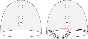
Suppose is an oriented Legendrian knot in a closed contact -manifold . Let
be the sutured contact manifold obtained by removing a standard neighborhood of from . Attaching a bypass to this knot complement along the arc shown in Figure 13 yields the knot complement with its two meridional sutures. We refer to this operation as a Stipsicz-Vértesi bypass attachment as it was studied extensively by those authors in [SV09]. Let us denote by
| (20) |
the sutured contact manifold obtained via this attachment. Inspired by [SV09, Theorem 1.1], we define the Legendrian invariant to be the contact invariant of this manifold.
2pt \pinlabel at 170 0
at 105 85 \pinlabel at 162 135
at 145 49
\endlabellist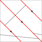
Definition 5.1.
Given a Legendrian knot , let
This class is by construction an invariant of the Legendrian knot type of .
Stipsicz and Vértesi observed in the proof of [SV09, Theorem 1.5] that the sutured contact manifold and therefore the class is invariant under negative Legendrian stabilization of . This then enables us to define an invariant of transverse knots in via Legendrian approximation as below since any two Legendrian approximations of a transverse knot are related by negative Legendrian stabilization.
Definition 5.2.
Given a transverse knot with Legendrian approximation , let
This class is an invariant of the transverse knot type of .
Remark 5.3.
Given a transverse knot with Legendrian approximation , we have
where
is the map our theory associates to the Stipsicz-Vértesi bypass attachment.
Below, we prove some results about the Legendrian invariant which will be important in Section 6. Our proofs are similar to those of analogous results in the monopole Floer setting [BS18, Siv12]. First, we establish the following notation.
Notation 5.4.
Given a closed contact 3-manifold , we will denote by the sutured contact manifold
obtained by removing a Darboux ball from , with dividing set consisting of a single curve on the boundary. In particular, we will write for the contact invariant of this sutured contact manifold.
The result below is an analogue of [BS18, Proposition 3.13].
Lemma 5.5.
Suppose is a Legendrian unknot with contained inside a Darboux ball in . Then there is an isomorphism
which sends to .
Proof.
Attaching a contact -handle to results in a sutured contact manifold of the form
The associated contact -handle attachment isomorphism
| (21) |
identifies with . (We recall from §2.2.3 that this isomorphism is merely the identity map on for some which is simultaneously a closure of both and .) It thus suffices to check that is isotopic to the contact structure used to define , obtained by removing a standard neighborhood of and attaching a Stipsicz-Vértesi bypass. Since we can arrange that this operation and the contact -handle attachment both take place in a Darboux ball, it suffices to check this in the case
But in this case, is a solid torus with two longitudinal sutures. As there is a unique isotopy class of tight contact structures on the solid torus with this dividing set, we need only check that and are both tight.
The class is nonzero since is Stein fillable [BS16b, Theorem 1.4]. It follows that is nonzero as well since the isomorphism (21) identifies this class with . This implies that is tight by Theorem 2.37.
The fact that is tight follows from the fact that the Heegaard Floer Legendrian invariant of the unknot in is nonzero, since this invariant agrees with the Heegaard Floer contact invariant of according to [SV09, Theorem 1.1]. (One can also prove tightness directly—i.e., without using Heegaard Floer homology—though it takes more room.) ∎
The result below follows immediately from Theorem 2.39.
Lemma 5.6.
Let and be disjoint Legendrian knots in , and let be the contact manifold obtained by contact -surgery on . If has image in then there is a homomorphism
which sends to .∎
At the level of closures of sutured manifolds, the homomorphism of Lemma 5.6 is simply the cobordism map on instanton homology associated to attaching a -dimensional 2-handle along , as described in §2.2.3.
Lemma 5.7.
Suppose is a Legendrian knot in and that is the result of contact -surgery on . Then there is a homomorphism
which sends to .
Proof.
Let be a Legendrian isotopic pushoff of with an extra positive twist around , as in Figure 14.
2pt
\pinlabel at 15 10
\pinlabel at 15 28
\endlabellist
The lemmas above culminate in Theorem 5.8 below, which is an analogue of [Siv12, Corollary 5.4] and [BS18, Corollary 3.16]. The exact triangle argument used in its proof was inspired by Lisca and Stipsicz’s proof of [LS04, Theorem 1.1]. We will use Theorem 5.8 in our proof of Theorem 1.18 in the next section, which states that is nonzero for transverse bindings of open books.
Theorem 5.8.
Suppose is a Legendrian knot in with 4-ball genus such that . Then
Proof.
Choose a Darboux ball disjoint from . Let denote the sutured contact manifold obtained by removing this ball from . Note that contact -surgery on results in a sutured contact manifold
which is topologically the result of -surgery on with respect to its Seifert framing, minus a ball. We have that is nonzero since is Stein fillable [BS16b, Theorem 1.4]. We will use the surgery exact triangle and the adjunction inequality to show that the map
| (22) |
defined in Section 2.2.3 is injective. But we know that
by Theorem 2.39. This will show that is nonzero as well, which will then imply that is nonzero by Lemma 5.7, proving the theorem.
Let be a closure of and let
be the tuples obtained from by performing - and -surgeries on with respect to its contact framing. These tuples are naturally closures of
respectively. As observed in (11), Theorem 2.10 gives us an exact triangle
where is the curve in corresponding to the meridian of , as in Figure 6, and moreover the map on is induced by .
Note that is topologically the same as the cobordism from to obtained from by attaching a -framed -handle along with respect to its Seifert framing. This cobordism contains a closed surface of genus and self-intersection
gotten by capping off the surface bounded by which attains
with the core of the -handle. The surface violates the adjunction inequality [KM95, Theorem 1.1], which implies that the map
Therefore,
is injective, and this means that the map in (22) is injective as well. This completes the proof of Theorem 5.8 as discussed above. ∎
6. Proof of Theorem 1.7
In this section we prove Theorem 1.7, restated below, as outlined in the introduction.
Theorem 1.7.
Suppose is a genus fibered knot in with fiber . Then .
Suppose for the rest of this section that is a fibered knot as in the hypothesis of Theorem 1.11. Let be an open book corresponding to the fibration of with supporting a contact structure on . We begin with some preliminaries.
Definition 6.1.
Given a properly embedded arc , we say that sends to the left at an endpoint if is not isotopic to and if, after isotoping so that it intersects minimally, is to the left of near , as shown in Figure 15.
This definition and the one below are due to Honda, Kazez, and Matić [HKM07].
Definition 6.2.
is not right-veering if it sends some arc to the left at one of its endpoints.
2pt
at 47 28 \pinlabel at 19 28 \pinlabel at 41 -3 \pinlabel at 65 57

Remark 6.3.
For the proof of Theorem 1.7, we may assume without loss of generality that the monodromy is not right-veering. Indeed, note that one of or is not right-veering since otherwise
If is right-veering then we use the fact that is invariant under reversing the orientation of and consider instead the knot with open book . We will make clear below where we are relying on the assumption that is not right-veering; most of the results in this section do not require it.
Remark 6.4.
Since is invariant under reversing the orientation of , it suffices to prove that
That is what we do in this section.
With these preliminaries out of the way, we may proceed to the proof of Theorem 1.7.
As the binding of the open book , the knot is naturally a transverse knot in . We may not be able to approximate by a Legendrian on a page of , but we can positively stabilize to an open book as in Figure 16, whose monodromy
is the composition of with a positive Dehn twist around the curve shown in the figure, and then let denote the Legendrian approximation of shown there on a page of . The fact that this can be made Legendrian is a consequence of the Legendrian realization principle [Hon00, Theorem 3.7], because the union of two pages of is a convex surface whose dividing set is the binding, and because is nonseparating in and hence a “non-isolating” curve in .
Since lies in a convex surface and is disjoint from the dividing curves , we have
where denotes the twisting of the contact planes along with respect to the framing given by . We observe that is obtained from by plumbing on a positive Hopf band, through which passes once, and so it follows that
| (23) |
We will see later (Remark 6.6) why this is important.
Let denote the positive/negative Legendrian stabilization of . In particular, is also a Legendrian approximation of . Let
denote the contact manifold with convex boundary and dividing set obtained by removing a standard neighborhood of from .
2pt
at 97 249 \pinlabel at 425 249
at 610 93
at 396 91
Recall from the previous section (Remark 5.3) that the transverse invariant is given by
where
is the map induced by a Stipsicz-Vértesi bypass attachment. In the case , this bypass is attached along the arc shown in Figure 17. Stipsicz and Vértesi also showed in the proof of [SV09, Theorem 1.5] that
by attaching a bypass along the arc shown in Figure 17. Letting
denote the associated bypass attachment map, as in the introduction, we have that
Recall from the introduction that our proof of Theorem 1.7 begins with the following lemma.
2pt \pinlabel at 170 0
at 105 85 \pinlabel at 162 135
at 75 115
\pinlabel at 145 49
\pinlabel at 448 132
\endlabellist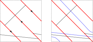
Lemma 1.16.
If the monodromy is not right-veering then
This in turn follows immediately from the lemma below, by Theorem 2.37.
Lemma 1.15.
If the monodromy is not right-veering then is overtwisted.
Remark 6.5.
Baker and Onaran proved in [BO15, Theorem 5.2.3] a similar result under the strictly stronger assumption that is the negative stabilization of another open book.
Proof of Lemma 1.15.
Suppose is not right-veering. Let be a properly embedded arc in with endpoints and such that sends to the left at . We can arrange that the -handle added to in forming the stabilization and the curve are as shown in the middle of Figure 18. Note in particular that intersects the Legendrian realization in one point and with negative sign.
2pt
at 106 258 \pinlabel at 434 257
at 769 254 \pinlabel at 233 118
at 620 100 \pinlabel at 955 98
at 208 68 \pinlabel at 118 68 \pinlabel at 396 96
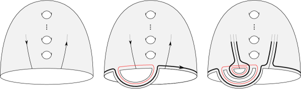
Given this setup, there is a standard way to realize on a page of the open book obtained by positively stabilizing , as shown in Figure 19. Namely, is given by the curve obtained by pushing along the arc and then over the -handle that was added in the stabilization. The right of Figure 18 provides another view of this realization .
2pt \pinlabel at 15 34
at 178 34 \pinlabel at 78 29
at 122 27
\pinlabel at 285 27
\pinlabel at 72 -1
\pinlabel at 72 50
\endlabellist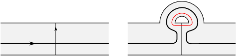
We now prove the remaining theorems which combine with Lemma 1.16 to prove Theorem 1.7, as outlined in the introduction. First, we have the following.
Theorem 1.17.
. In other words, the class is supported in Alexander grading .
Proof.
We will first prove that
| (24) |
As in Example 2.33, a partial open book for the complement is given by
Let be a basis for such that the endpoints of the basis arcs intersect as shown in the middle of Figure 20. Let
be the corresponding curves on the boundary of as defined in (10), so that
is obtained from
by attaching contact -handles along the . By Definition 2.34, the element is then the image of the generator
under the map associated to these -handle attachments.
2pt
at 218 33 \pinlabel at 538 33 \pinlabel at 33 52 \pinlabel at 360 52 \pinlabel at 520 75 \pinlabel at 470 5
at 790 5
\endlabellist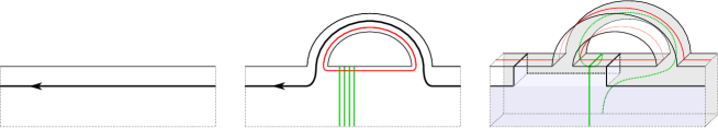
We claim that
| (25) |
To prove this, we let be a closure of adapted to a properly embedded copy of in as shown on the right of Figure 20. Let us assume that this closure is formed using an annular auxiliary surface. That is, to form we first form a preclosure by gluing a thickened annulus to in such a way that extends to a surface in obtained from by adding a -handle, as shown in the lower left of Figure 21.
2pt
\pinlabel at 510 145
\endlabellist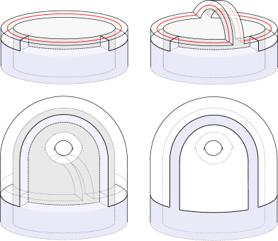
Then is defined to be and is formed by gluing to as specified by a diffeomorphism
which identifies the two boundary components
of . The surface caps off in to a closed surface , which is the union of with the annulus
We claim that and differ in by a torus. Indeed, if we remove the annulus from we recover , which is isotopic to the subsurface of shown in blue in the lower right of Figure 21. The union of this subsurface with the white annulus is equal to . So, the difference is homologous to the torus obtained as the union of these two annuli. Note that
By definition, then, the class is an element of the generalized -eigenspace of the operator
Corollary 2.9 then implies that it is also an element of the generalized -eigenspace of the operator
since and differ by a torus. But the latter eigenspace is, by definition, . This implies that lies in Alexander grading , as claimed in (25).
To show that lies in Alexander grading , as in (24), recall that on the level of closures, this class is the image of under the map induced by the cobordism associated to -framed surgeries on . The right of Figure 20 shows that these curves do not intersect the surface in , which means that they are disjoint from the capped off surface . This means that the capped off surfaces defining the Alexander gradings on the two ends of this cobordism are isotopic in the cobordism. Lemma 2.6 then implies the cobordism map respects the Alexander grading, which proves the claim.
To complete the proof of Theorem 1.17, we need only show that the bypass attachment map preserves Alexander grading, keeping in mind that
The argument for this is the same as above. The map is the composition of the maps associated to attaching a -handle with feet at the endpoints of the arc in Figure 17 and then attaching a -handle along the union of with an arc passing once over this 1-handle. Call this union . Suppose is a closure of the manifold obtained after the -handle attachment, adapted to . Then it is also a closure of , and, on the level of closures, is induced by the cobordism associated to surgery on . The right of Figure 17 shows that the arc does not intersect the surface , which implies that the surgery curve is disjoint from the capped off surface . This cobordism map therefore respects the Alexander grading, as argued above, which proves the claim. ∎
Remark 6.6.
It was important at the end of the proof of Theorem 1.17 that the arc was disjoint from the surface . This claim relied on the depiction of in Figure 17, so it behooves us to justify this depiction. This is where the observation
in (23) comes into play. First, this condition implies that
These two Thurston-Bennequin calculations then imply that each component of and intersects in and points, respectively. This forces to be as indicated in Figure 17.
Next, we prove the following analogue of Vela-Vick’s theorem [VV11] that the connected binding of an open book has nonzero transverse invariant in Heegaard Floer homology.
Theorem 1.18.
is nonzero.
Proof.
We first show that there is some genus fibered knot with open book such that the corresponding transverse invariant is nonzero. We then use the surgery exact triangle to show that there is an isomorphism
| (26) |
for any two such fibered knots which sends to Theorem 1.18 will follow.
For the first, let be the braid with two strands and positive crossings. Note that has genus . As a positive braid, is fibered with , with open book supporting the tight contact structure on . As the transverse binding of this open book, we have that
Let be the Legendrian representative of shown in Figure 22. We have that
Theorem 5.8 therefore implies that
We claim that is a Legendrian approximation of . For this, simply note that the transverse pushoff of has self-linking number
The transverse simplicity of torus knots, proven by Etnyre and Honda [EH01], then implies that is transversely isotopic to the transverse binding . In other words, is a Legendrian approximation of . It then follows that
is nonzero, as desired.
at 60 45 \pinlabel at 64.8 31.5

Suppose next that is a genus fibered knot with open book . Let be the fibered knot corresponding to the open book , where is a positive Dehn twist around a nonseparating curve . We first prove the isomorphism (26) for this pair.
Note that can be viewed as a Legendrian knot in the contact structure on corresponding to , with contact framing equal to the framing induced by . In this case, is the result of contact -surgery on . Let
be the sutured contact manifolds obtained by removing standard neighborhoods of Legendrian approximations and of and and attaching Stipsicz-Vértesi bypasses, as described in the previous section. Then is naturally a Legendrian knot in the first of these sutured contact manifolds, as is a subsurface of a page of a partial open book for this contact manifold. The second sutured contact manifold above is the result of contact -surgery on . Moreover, we have that
| (27) |
as per Remark 5.3.
Let be a closure of adapted to . Let
be the tuples obtained from by performing - and -surgery on with respect to the framing induced by . These are naturally closures of the sutured manifolds
adapted to in each case. By Theorem 2.10, there is a surgery exact triangle
as in (11), where is the curve in corresponding to the meridian of .
We can push slightly off of to ensure that the capped off surfaces in these closures are isotopic in the cobordisms between them. Lemma 2.6 then implies that the maps in this exact triangle respect the eigenspace decompositions associated with the operators . In particular, we have an exact triangle
where the third group denotes the generalized -eigenspace of the operator acting on . But the surface is homologous in to a surface of genus
obtained by surgering along , so Proposition 2.4 tells us that this -eigenspace is trivial. The map is therefore an isomorphism. Recall that this map gives rise to the map we denote by in Section 2.2.3. We have shown above that restricts to an isomorphism
Finally, since any two genus fibered knots and with fiber have open books with monodromies related by positive and negative Dehn twists around nonseparating curves in , we conclude that there is for any two such knots an isomorphism
sending to As discussed above, this completes the proof of Theorem 1.18. ∎
The bypass attachment along the arc in Figure 17 fits into a bypass triangle as shown in Figure 23. Note that the arc of attachment in the upper right is precisely the arc defining the Stipsicz-Vértesi bypass attachment which induces the map .
2pt
at 402 370 \pinlabel at 459 420
at 782 370 \pinlabel at 905 421
at 837 420
\pinlabel at 345 428
\pinlabel at 578 452
\pinlabel at 758 261
\pinlabel at 410 260
\endlabellist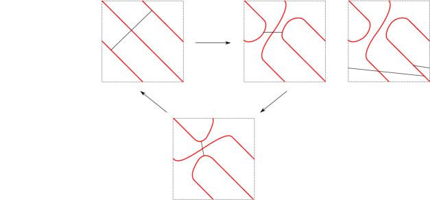
By Theorem 1.21, there is a corresponding bypass exact triangle of the form
| (28) |
To prove Theorem 1.7, let us now assume that the monodromy is not right-veering. Then
by Lemma 1.16. Exactness of the triangle (28) then tells us that there is a class
such that
The composition
| (29) |
therefore satisfies
| (30) |
which is nonzero by Theorem 1.18. Thus, is nonzero.
The class is not a priori homogeneous with respect to the Alexander grading on . However, we prove the following, which completes the proof of Theorem 1.7.
Theorem 6.7.
The component of in is nonzero.
Proof.
The composite map is ultimately induced by a cobordism
from a closure
to another closure
corresponding to surgery on curves away from the embedded copies of in these . We can arrange that these two closures are adapted to . The capped off surfaces and in these closures are unions of with once-punctured tori,
The surfaces are isotopic within as they are contained on the boundary of a product region
We therefore have that
| (31) |
in , where is the genus two surface in with self-intersection given as the union
of these once-punctured tori. Let be the element representing the class Write
where . We know from (30) that the map sends to a representative of , which must be a nonzero element of by Theorems 1.17 and 1.18. It follows from Proposition 2.8 and the relation (31), however, that the only components of whose images can have nonzero components in are and , since . On the other hand, we claim that
This will prove that must be nonzero, proving the theorem. For this claim, note that
since is fibered. This group is therefore generated by by Theorems 1.17 and 1.18. If is zero then we are done. If not, then represents a nonzero multiple of , so
Thus, it remains to show that the latter is zero. For this, recall that
It then follows that
by the exactness of the triangle (28). ∎
References
- [BO15] Kenneth L. Baker and Sinem Onaran. Nonlooseness of nonloose knots. Algebr. Geom. Topol., 15(2):1031–1066, 2015.
- [BS15] John A. Baldwin and Steven Sivek. Naturality in sutured monopole and instanton homology. J. Differential Geom., 100(3):395–480, 2015.
- [BS16a] John A. Baldwin and Steven Sivek. A contact invariant in sutured monopole homology. Forum Math. Sigma, 4:e12, 82, 2016.
- [BS16b] John A. Baldwin and Steven Sivek. Instanton Floer homology and contact structures. Selecta Math. (N.S.), 22(2):939–978, 2016.
- [BS18] John A. Baldwin and Steven Sivek. Invariants of Legendrian and transverse knots in monopole knot homology. J. Symplectic Geom., 16(4):959–1000, 2018.
- [BVV18] John Baldwin and David Shea Vela-Vick. A note on the knot Floer homology of fibered knots. Algebr. Geom. Topol., 18(6):3669–3690, 2018.
- [DG09] Fan Ding and Hansjörg Geiges. Handle moves in contact surgery diagrams. J. Topol., 2(1):105–122, 2009.
- [DK90] S. K. Donaldson and P. B. Kronheimer. The geometry of four-manifolds. Oxford Mathematical Monographs. The Clarendon Press, Oxford University Press, New York, 1990. Oxford Science Publications.
- [Don02] S. K. Donaldson. Floer homology groups in Yang-Mills theory, volume 147 of Cambridge Tracts in Mathematics. Cambridge University Press, Cambridge, 2002. With the assistance of M. Furuta and D. Kotschick.
- [EH01] John B. Etnyre and Ko Honda. Knots and contact geometry. I. Torus knots and the figure eight knot. J. Symplectic Geom., 1(1):63–120, 2001.
- [Etn03] John B. Etnyre. Introductory lectures on contact geometry. In Topology and geometry of manifolds (Athens, GA, 2001), volume 71 of Proc. Sympos. Pure Math., pages 81–107. Amer. Math. Soc., Providence, RI, 2003.
- [Etn06] John B. Etnyre. Lectures on open book decompositions and contact structures. In Floer homology, gauge theory, and low-dimensional topology, volume 5 of Clay Math. Proc., pages 103–141. Amer. Math. Soc., Providence, RI, 2006.
- [EVVZ17] John B. Etnyre, David Shea Vela-Vick, and Rumen Zarev. Sutured Floer homology and invariants of Legendrian and transverse knots. Geom. Topol., 21(3):1469–1582, 2017.
- [Gei08] Hansjörg Geiges. An introduction to contact topology, volume 109 of Cambridge Studies in Advanced Mathematics. Cambridge University Press, Cambridge, 2008.
- [Gir91] Emmanuel Giroux. Convexité en topologie de contact. Comment. Math. Helv., 66(4):637–677, 1991.
- [Gir00] Emmanuel Giroux. Structures de contact en dimension trois et bifurcations des feuilletages de surfaces. Invent. Math., 141(3):615–689, 2000.
- [HKM07] Ko Honda, William H. Kazez, and Gordana Matić. Right-veering diffeomorphisms of compact surfaces with boundary. Invent. Math., 169(2):427–449, 2007.
- [HKM08] Ko Honda, William H. Kazez, and Gordana Matić. Contact structures, sutured Floer homology, and TQFT. Preprint, arXiv:math/0807.2431v1[math.GT], 2008.
- [HKM09] Ko Honda, William H. Kazez, and Gordana Matić. The contact invariant in sutured Floer homology. Invent. Math., 176(3):637--676, 2009.
- [Hon00] Ko Honda. On the classification of tight contact structures. I. Geom. Topol., 4:309--368, 2000.
- [HW18] Matthew Hedden and Liam Watson. On the geography and botany of knot Floer homology. Selecta Math. (N.S.), 24(2):997--1037, 2018.
- [KM95] P. B. Kronheimer and T. S. Mrowka. Gauge theory for embedded surfaces. II. Topology, 34(1):37--97, 1995.
- [KM10a] Peter Kronheimer and Tom Mrowka. Instanton Floer homology and the Alexander polynomial. Algebr. Geom. Topol., 10(3):1715--1738, 2010.
- [KM10b] Peter Kronheimer and Tomasz Mrowka. Knots, sutures, and excision. J. Differential Geom., 84(2):301--364, 2010.
- [KM11] P. B. Kronheimer and T. S. Mrowka. Khovanov homology is an unknot-detector. Publ. Math. Inst. Hautes Études Sci., (113):97--208, 2011.
- [Krc15] David Krcatovich. The reduced knot Floer complex. Topology Appl., 194:171--201, 2015.
- [LOSS09] Paolo Lisca, Peter Ozsváth, András I. Stipsicz, and Zoltán Szabó. Heegaard Floer invariants of Legendrian knots in contact three-manifolds. J. Eur. Math. Soc. (JEMS), 11(6):1307--1363, 2009.
- [LS04] Paolo Lisca and András I. Stipsicz. Ozsváth-Szabó invariants and tight contact three-manifolds. I. Geom. Topol., 8:925--945, 2004.
- [Mas14] Patrick Massot. Topological methods in 3-dimensional contact geometry. In Contact and symplectic topology, volume 26 of Bolyai Soc. Math. Stud., pages 27--83. János Bolyai Math. Soc., Budapest, 2014.
- [Muñ99] Vicente Muñoz. Ring structure of the Floer cohomology of . Topology, 38(3):517--528, 1999.
- [Ozb11] B. Ozbagci. Contact handle decompositions. Topology Appl., 158(5):718--727, 2011.
- [Sca15] Christopher W. Scaduto. Instantons and odd Khovanov homology. J. Topol., 8(3):744--810, 2015.
- [Siv12] Steven Sivek. Monopole Floer homology and Legendrian knots. Geom. Topol., 16(2):751--779, 2012.
- [SV09] András I. Stipsicz and Vera Vértesi. On invariants for Legendrian knots. Pacific J. Math., 239(1):157--177, 2009.
- [VV11] David Shea Vela-Vick. On the transverse invariant for bindings of open books. J. Differential Geom., 88(3):533--552, 2011.