$SU(2)$ Yang-Mills solitons in $R^{2}$ gravity

Abstract

We construct new family of spherically symmetric regular solutions of $SU(2)$ Yang-Mills theory coupled to pure $R^{2}$ gravity. The particle-like field configurations possess non-integer non-Abelian magnetic charge. A discussion of the main properties of the solutions and their differences from the usual Bartnik-McKinnon solitons in the asymptotically flat case is presented. It is shown that there is continuous family of linearly stable non-trivial solutions in which the gauge field has no nodes.

I Introduction

Modified theories of gravity gained increasing interest in past decade since it now seems accepted that the inflationary scenario in the early Universe is related with modification of the usual Einstein-Hilbert action Starobinsky:1980te , in particular via addition of the quadratic curvature terms. The simplest $R+R^{2}$ model Salam:1978fd is proven to be renormalizable Stelle:1976gc ; Stelle:1977ry , further, it appears in a natural way as a limit of the string theory Ellis:2013xoa . Such generalizations have been also studied as an explanation for the dark energy problem Capozziello:2002rd ; Starobinsky:2007hu .

The linear Einstein term is not always assumed to be present in the action of the modified gravity. The pure $R^{2}$ theory has some advantages Kounnas:2014gda ; Alvarez-Gaume:2015rwa , in particular it is the only ghost-free higher order theory. On the other hand, it admits supergravity generalization Ferrara:2015ela ; Kuzenko:2016nbu . Further, pure $R^{2}$ black hole and wormhole solutions were constructed in Kehagias:2015ata ; Duplessis:2015xva , very recently the pure $R^{2}$ theory supplemented by a set of complex scalar fields was investigated in Ellis:2017xwz as a limit of supergravity model. However, not much known about solutions of the $R^{2}$ gravity coupled to the non-Abelian fields.

Spatially localised particle-like solutions of the classical Yang-Mills theory coupled to the usual gravity have been the subject of long standing research interest since Bartnik and McKinnon found these solutions in 1988 Bartnik:1988am . These globally regular self-gravitating field configurations were discovered numerically in the asymptotically flat $\mbox{SU}(2)$ Einstein-Yang-Mills (EYM) theory. It has been shown that they are linked to the nontrivial hairy black holes Volkov:1989fi ; Bizon:1990sr , this observation sparked a lot of activity over last two decades, see e.g. Volkov:1998cc ; Volkov:2016ehx . The $\mbox{SU}(2)$ Bartnik-McKinnon (BM) solutions in the asymptotically flat space are spherically symmetric and purely magnetic with the net magnetic charge equal to zero Galtsov:1989ip ; Bizon:1992pi , further they are unstable with respect to linear perturbations of the metric and the gauge field Straumann:1989tf ; Zhou:1991nu ; Lavrelashvili:1994rp . The BM solutions were subsequently generalized to the $\mbox{SU}(N)$ Kuenzle:1991wa ; Brodbeck:1994np ; Kleihaus:1995tk and the $\mbox{SO}(N)$ Bartnik:2009hc ; Oliynyk:2000vf Einstein-Yang-Mills theory, axially symmetric generalizations of the BM solutions were considered in Kleihaus:1996vi ; Ibadov:2004rt .

An interesting observation is that a variety of features of asymptotically flat self-gravitating BM solutions and the corresponding hairy black holes are not shared by their counterparts in the asymptotically anti-de Sitter (AdS) space-time Winstanley:1998sn ; Bjoraker:1999yd ; Bjoraker:2000qd ; Sarbach:2001mc . There is a continuum of new magnetically charged field configurations with asymptotically non-vanishing magnetic flux, which are stable under linear perturbations of the fields. One can consider these solutions as describing non-Abelian monopoles in the absence of a Higgs field with a non-integer magnetic charge Bjoraker:1999yd ; Bjoraker:2000qd . On the other hand, these solutions are relevant in the context of the AdS/QFT holographical correspondence Gubser:2008wv . As discussed in Baxter:2007au ; Winstanley:2008ac , the EYM solutions in AdS₄ spacetime possess generalizations with higher gauge groups, there is also variety of interesting axially-symmetric AdS solutions of the EYM equations Radu:2001ij ; Kichakova:2014fta .

The main purpose of this work is to explicitly construct $R^{2}$ counterparts of the spherically symmetric solutions of the EYM system, looking for new features induced by the different structure of the gravitational part of the action.

II $R^{2}$ Yang-Mills model

We consider the $\mbox{SU}(2)$ Yang-Mills gauge field coupled to pure $R^{2}$ gravity in $(3+1)$ dimensions. The model is defined by the scale invariant action

$$S=\int\sqrt{-g}\left(\frac{R^{2}}{2\kappa}-{\rm Tr}\;F_{\mu\nu}F^{\mu\nu}\right)d^{4}x$$ (1)

where $R$ is the usual curvature scalar, $g$ denotes the determinant of the metric $g_{\mu\nu}$ and $\kappa$ is the effective gravitational coupling constant. The matter field sector is defined by the $\mbox{SU}(2)$ field strength tensor

$$F_{\mu\nu}=\partial_{\mu}A_{\nu}-\partial_{\nu}A_{\mu}-i[A_{\mu},A_{\nu}]\,,$$

and $A_{\mu}=\frac{1}{2}A_{\mu}^{a}\tau^{a}\in\mathfrak{su}(2)$.

It is known the pure $R^{2}$ theory is equivalent to the usual Einstein gravity with additional real scalar field Kounnas:2014gda . Indeed, one can replace the $R^{2}$ term with $\frac{R^{2}}{\kappa}\to 2tR-\kappa t^{2}$, where $t$ is a Lagrange multiplier. Then the variational equation for the field $t$, which is non-propagating in this frame, yields the $R^{2}$ term back. Consequent rescaling of the metric to the Einstein frame and redefinition of the field $t\to\phi\sim\ln(2t)$, transforms the pure $R^{2}$ gravity to the standard gravitational action with a cosmological constant, coupled to a massless scalar field $\phi$ Kounnas:2014gda .

The scale invariant model (1) in the Einstein frame after rescaling takes the form

$$S=\int\sqrt{-g}\left(\frac{1}{2}R-\frac{1}{2}\partial_{\mu}\phi\partial^{\mu}\phi-\frac{\kappa}{8}-{\rm Tr}\;F_{\mu\nu}F^{\mu\nu}\right)d^{4}x$$ (2)

Here the quantity $\frac{\kappa}{4}$ is playing the role of the cosmological constant.

Such a theory, with positive cosmological constant and both scalar and non-Abelian Yang-Mills fields in the matter sector, is not very common, Most attention is usually devoted to similar models with an exponential dilaton coupling, see e.g. Lavrelashvili:1992ia ; Kleihaus:1996vi ; Radu:2004xp . On the other hand, the reformulated model in the Einstein frame may only capture part of the possible solutions of the original theory with $R^{2}$ term Kehagias:2015ata , so hereafter we restrict our consideration to the model (1).

Variation of the action (1) with respect to the metric $g_{\mu\nu}$ yields the $R^{2}$ gravity equations, which are counterparts of the usual Einstein equations:

$$RR_{\mu\nu}-\frac{1}{4}R^{2}g_{\mu\nu}-\nabla_{\mu}\nabla_{\nu}R+g_{\mu\nu}\square R=\frac{\kappa}{2}T_{\mu\nu}\,.$$ (3)

Here the Yang-Mils stress-energy tensor is

$$T_{\mu\nu}=-4\;{\rm Tr}\left(F_{\mu\rho}F_{\nu}^{\rho}-\frac{1}{4}g_{\mu\nu}F^{\rho\sigma}F_{\rho\sigma}\right)\,.$$ (4)

Variation of the action (1) with respect to the gauge field $A_{\mu}$ leads to the Yang-Mills equations in the curved space-time

$$\nabla_{\mu}F^{\mu\nu}-i[A_{\mu},F^{\mu\nu}]=0$$ (5)

Note that the equations of $R^{2}$ gravity (3) are highly non-linear fourth order differential equations, it is not obvious how such a system can be integrated in a general case. However, we can see that the left hand side of the gravitational equations (3) is covariantly constant, thus Kehagias:2015ata

$$\nabla^{\mu}T_{\mu\nu}=0\,.$$ (6)

Further, the action (1) is classically scale invariant, i.e. ${\rm Tr}\;T_{\mu\nu}=0$. Taking trace on both sides of the Eq. (3) we obtain

$$\square R=0\,.$$ (7)

Thus, in the static case the regular solutions of the Laplace equation (7) on the entire space $\mathbb{R}^{3}$ without event horizon, are harmonic functions. In such a case the Liouville’s theorem guarantees that $R=\textrm{const}$ is a solutions of Eq. (7). This result greatly simplifies the consideration, indeed there are two distinct situations. In the case of zero curvature, the solutions of the model (1) in the asymptotically flat spacetime are trivial and $T_{\mu\nu}=0$. In the second case we suppose that the scalar curvature is a non-vanishing constant. Then the $R^{2}$ gravitational equation (3) can be written in the Einsteinian form

$$R_{\mu\nu}-\frac{1}{4}g_{\mu\nu}R=\frac{\kappa}{2R}T_{\mu\nu}\,.$$ (8)

Since the curvature scalar is a constant, solutions of this equation are given by the equivalent Einstein equations in the AdS spacetime upon identification $R=4\Lambda$ and rescaling of the gravitational coupling constant as $\kappa\to\frac{\kappa}{8\Lambda}$.

II.1 Spherically symmetric ansatz and the boundary conditions

We restrict our consideration to the static spherically symmetric field configuration, which are counterparts of the usual BM solutions. Then the spherically symmetric purely magnetic Ansatz for the Yang-Mill field is given by

$$A_{0}=0\,;\qquad A_{i}^{a}=\varepsilon^{a}_{ij}\frac{x_{j}}{r^{2}}\left(1-w(r)\right)\,,$$ (9)

where $w(r)$ is the profile function. For the metric, we employ the usual spherically symmetric line element

$$ds^{2}=-\sigma^{2}(r)N(r)dt^{2}+\frac{dr^{2}}{N(r)}+r^{2}\left(d\theta^{2}+\sin^{2}\theta~{}d\phi^{2}\right)\,.$$ (10)

Within this specific ansatz (10), the Laplace equation (7) becomes

$$\frac{R_{rr}}{R_{r}}+\frac{N_{r}}{N}+\frac{\sigma_{r}}{\sigma}+\frac{2}{r}=0\,.$$ (11)

A general solution of this equation can be written as

$$R=C_{1}+C_{2}\int\limits_{0}^{\infty}\frac{dr}{r^{2}\sigma N}\,,$$

where $C_{1},C_{2}$ are two arbitrary constants. The regularity condition yields $C_{2}=0$, as it is mentioned above, the curvature scalar is a constant.

Note that in the case of positive constant curvature, the spherically-symmetric solutions of the Yang-Mills system coupled to $R^{2}$ gravity are effectively equivalent to the asymptotically de-Sitter solutions in the Yang-Mills model coupled to the usual Einstein gravity Volkov:1996qj . This is not the case, however, for the asymptotically AdS solutions with a negative constant curvature, $R<0$. In the Einstein gravity this situation would correspond to a non-conventional choice of the negative gravitational coupling constant. Hereafter we consider the case of $R<0$.

As we can see, this equivalence also holds for a theory (2) in the Jordan frame. Indeed, in the case of constant scalar curvature the scalar field $\phi$ should also be constant, the corresponding dynamical equation is just $\square\phi=0$ and the field $\phi$ is constant everywhere in space. Thus, it does not affect the dynamical equations for the metric functions and the Yang-Mills field, in the Jordan frame the scalar field is effectively decoupled.

Within the spherically symmetric ansatz (9),(10), the variational equations associated with the action (1) can be reduced to the following system of three non-linear differential equations

$$\begin{split}w_{rr}&=w_{r}\frac{r^{2}R[r^{2}R+4(N-1)]+2\kappa(w^{2}-1)^{2}}{4NRr^{3}}+\frac{w(w^{2}-1)}{Nr^{2}}\,,\\ N_{r}&=-\frac{\kappa(w^{2}-1)^{2}}{2Rr^{3}}+\frac{R[Rr^{2}+4(N-1)]+4\kappa Nw_{r}^{2}}{4Rr}\,,\\ \sigma_{r}&=\frac{\kappa\sigma w_{r}^{2}}{Rr}\,.\end{split}$$ (12)

Note that the metric function $\sigma(r)$ can be integrated out,

$$\sigma(r)=\sigma(0)\exp\left(\frac{\kappa}{R}\int_{0}^{\infty}\frac{w_{r}^{2}}{r}dr\right)\,.$$

The series expansion of the equations (12) near the origin yields

$$\begin{split}w&\approx 1-br^{2}+O(r^{4})\,,\\ \sigma&\approx\sigma_{0}+\frac{2\kappa b^{2}}{R}+O(r^{4})\,,\\ N&\approx 1-\left(\frac{2\kappa b^{2}}{R}+\frac{R^{2}}{12}\right)r^{2}+O(r^{4})\,.\end{split}$$ (13)

Similarly, on the spacial boundary

$$\begin{split}w&\approx w_{\infty}-\frac{6w_{\infty}(w_{\infty}^{2}-1)}{Rr^{2}}+O(r^{-4})\,,\\ \sigma&\approx 1+O(r^{-4})\,,\\ N&\approx 1-\frac{R}{12}r^{2}-\frac{2M}{r}+\frac{\kappa(w_{\infty}^{2}-1)^{2}}{2Rr^{2}}+O(r^{-3})\,.\end{split}$$ (14)

Here $\sigma_{0},M$ and $w_{\infty}$ are constants that have to be determined numerically. The constants $\kappa$ and $b$ are the parameters of a particular spherically-symmetric solutions of the $R^{2}$ Yang-Mills coupled system.

Thus, in order to obtain regular solutions of this model with finite energy density we have to impose the following boundary conditions

$$w(0)=1\,,\quad w_{r}(0)=0\,,\quad N(0)=0\,\quad\sigma(\infty)=1\,.$$ (15)

Evidently, they agree with the corresponding boundary conditions for the asymptotically AdS EYM system, see Bjoraker:1999yd .

The static regular localized solutions are characterized by the mass $\mathcal{M}$ and by the non-Abelian magnetic charge

$$Q=\frac{1}{4\pi}\int\sqrt{-g}\varepsilon^{ijk}F_{ij}dS_{k}=(1-w_{\infty}^{2})\frac{\tau_{3}}{2}\,.$$ (16)

For the gauge invariant charge we use the definition $|Q|$, where the vertical bars denote the Lie-algebra norm Sudarsky:1992ty . Similar to the asymptotically AdS solutions in the usual EYM system Winstanley:1998sn ; Bjoraker:1999yd ; Bjoraker:2000qd ; Sarbach:2001mc , the function $w(r)$ does not need to have an asymptotic value $w_{\infty}=\pm 1$, the charge (16) generally is not integer.

Note that by analogy with the corresponding solutions in the AdS₄ spacetime, we can reparametrize the metric function $N(r)$ as

$$N(r)=1-\frac{2m(r)}{r}-\frac{Rr^{2}}{12}\,,$$ (17)

where the function $m(r)$ has an asymptotic limit $m(\infty)=M$. However, in the $R^{2}$ gravity the usual definition of the Arnowitt-Deser-Misner mass should be modified in the comparison with the case of the conventional general relativity Deser:2002rt . Thus, the parameter $M$ does not uniquely specify the mass, in the system under consideration the static energy is defined as $\mathcal{M}=MR$ instead Deser:2002rt ; Deser:2007vs .

III Numerical results

Solutions for system of equations (12) with boundary conditions (15) are constructed numerically using shooting algorithm, based on Dormand-Prince 8th order method with adaptive stepsize. The relative errors of calculations are lower than $10^{-10}$. Similar to the case of the soliton solutions in the usual EYM model, for each fixed values of the parameter $\kappa$ there is a continuous set of regular magnetic solutions labeled by the free adjustable parameter $b$. Typical solutions are displayed in Fig. 1. For all the solutions we present we make use of the scale invariance of the model (1) and take the value of the curvature scalar $R=-1$.

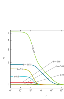
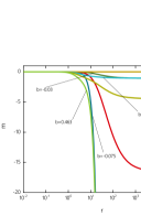
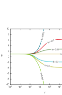
Figure 1: $R^{2}$ EYM solutions for $R=-1$, $\kappa=1$ and some set of values of $b$: The metric function $\sigma(r)$ (upper left plot), the mass function $m(r)$ (upper right plot) and the profile function of the gauge field $w(r)$ (bottom plot) are plotted as functions of the radial coordinate $r$.

Variation of the shooting parameter $b$ gives us a continuous family of solutions, which are qualitatively similar to the usual Einstein-Yang-Mills monopoles in asymptotically AdS spacetime Bjoraker:1999yd ; Bjoraker:2000qd . However, there are some important differences. First, the regular finite energy $R^{2}$ EYM magnetic solutions exist only for one finite interval of values of the parameter $b$ bounded from above and below, $b\in[b_{min},b_{max}]$ where $b_{min}<0$. Contrary to this case, a continuum of monopole solutions in the conventional EYM AdS₄ exists for all values of the shooting parameter bounded from above only Bjoraker:1999yd ; Bjoraker:2000qd . On the other hand, the family of finite energy EYM solutions in the fixed AdS background also exist for only one interval in parameter space Radu:2001ij . Secondly, there is an additional parameter labeling the usual EYM AdS₄ solutions, the number $n$ of oscillations of the Yang-Mills field. Our numerical results show that for the $R^{2}$ EYM system there are only solutions with $n=0$ or $n=1$. Thus, although the $R^{2}$ gravity coupled to the Yang-Mills theory can be conformally transformed to Einstein frame, where it takes the form of the standard Einstein gravity with cosmological constant and both massless scalar and non-Abelian Yang-Mills fields in the matter sector, the solutions of these models are still quite different, there is no one-to-one correspondence between them.

Setting the shooting parameter $b=0$ yields the trivial zero energy solution with vanishing non-Abelian magnetic field in the AdS space with a cosmological constant $\Lambda=\frac{R}{4}$. Increasing of the parameter $b$ lead to increase of both the energy and the magnetic charge of the configuration. These solutions are of particular interest because, as we will see below, they are stable against linear perturbations. At some value of $b$ the asymptotic value of the gauge field function $w_{\infty}$ approaches zero and the magnetic charge takes its maximal value, $|Q|=1$. Further increase of the parameter $b$ leads to decrease of the charge which again deviates from an integer, on this unstable branch of solutions the gauge field profile function $w(r)$ has a single node. At some upper critical value of the parameter $b$ both the mass and the energy diverge, see Fig. 2

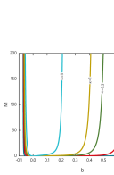
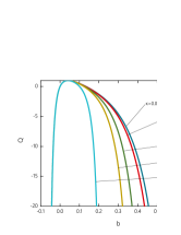
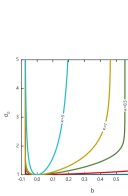
Figure 2: The energy (upper left plot), the magnetic charge (upper right plot) and the value of the metric function $\sigma_{0}=\sigma(0)$ (bottom plot) of $R^{2}$ EYM solutions are shown as functions of the parameter $b$ for some set of values of the gravitational coupling $\kappa$ at $R=-1$.

Similarly, decreasing of the parameter $b$ from zero is leading to decrease of the magnetic charge of the configuration, along this branch the energy rapidly increases, both the energy and the charge diverge at some negative value of $b=b_{min}$. No solution seems to exist for $b$ less than this value. Note that the pattern of critical behavior is different from the usual EYM monopoles, the metric function $N$ of the $R^{2}$ EYM solutions diverge at both extremities of the interval of values of $b$, while it approaches zero in the case of the EYM AdS₄ solutions Bjoraker:2000qd . As shown in Fig. 2, the interval of values of the parameter $b$ decreases when the gravitational coupling constant $\kappa$ gets larger. The contraction of this interval is mainly because of decrease of the upper critical value $b_{max}$, the lower critical value $b_{min}$ weakly depends on variations of the coupling constant $\kappa$. Dependencies of the critical values of the parameter $b$ on $\kappa$ are shown in Fig. 3. Both critical values, $b_{max}$ and $b_{min}$, approach zero as $\kappa$ tends to infinity, however the upper critical value $b_{max}$ decreases monotonically, while the lower critical value $b_{min}$ possesses a minimum at $\kappa\sim 6$.

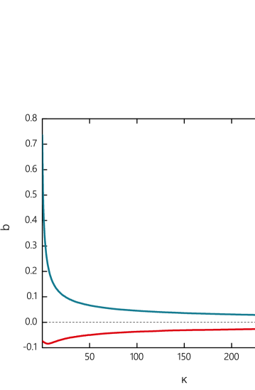
Figure 3: Critical values of the parameter $b$ are shown as functions of the effective gravitational coupling constant $\kappa$ for $R=-1$.

IV Linear stability analysis

In is known that the usual EYM AdS₄ magnetic solutions with no node in $w(r)$ are stable with respect to linear perturbations Bjoraker:1999yd ; Bjoraker:2000qd , so we can expect the same arguments can be applied to the corresponding solutions of the $R^{2}$ EYM system. We consider small time-dependent perturbations of the configuration (9) described by the general magnetic ansatz for the spherically symmetric Yang-Mills connection

$$A=\frac{1}{2}\left\{u(r,t)\tau_{3}dr+[w(r,t)\tau_{1}+v(r,t)\tau_{2}]d\theta+[w(r,t)\tau_{2}-v(r,t)\tau_{1}+\cot\theta\tau_{3}]\sin\theta d\phi\right\}\,.$$ (18)

It is more convenient in the stability analysis to make use of the following parametrization for the metric

$$ds^{2}=-e^{\nu(r,t)}N(r,t)dt^{2}+e^{\lambda(r,t)}dr^{2}+r^{2}(d\theta^{2}+\sin^{2}\theta d\phi^{2})\,,$$ (19)

instead of (10).

The functions in this general ansatz can be now written as the sum of the static solution, which stability we are investigating, and a time dependent perturbations:

$$\begin{split}w(r,t)&=w(r)+\delta w(r,t)\,,\qquad u(r,t)=\delta u(r,t)\,,\qquad v(r,t)=\delta v(r,t)\,;\\ \nu(r,t)&=\nu(r)+\delta\nu(r,t)\,,\qquad\lambda(r,t)=\lambda(r)+\delta\lambda(r,t)\,.\end{split}$$ (20)

Substituting (20) into the action of the system (1) and retaining only terms linear in perturbations, we variate the corresponding functional with respect to the fluctuations of the matter fields $\delta w,\delta u$ and $\delta v$. The equations for fluctuations of the metric fields can be obtained from the linearized gravitational equations (8). In particular, integration of the corresponding $rt$-equation over time yields the relation

$$\delta\lambda=\frac{2\kappa w_{r}}{Rr}\delta w\,.$$

Another relation between the perturbations can be obtained from the linear combination of the $tt$- and $rr$- Einsteinian equations, together with the corresponding unperturbed equations:

$$\delta\lambda_{r}+\delta\nu_{r}=\frac{4\kappa w_{r}}{Rr}\delta w\,.$$

With there relations at hands, we arrive to the following system of the linearized equations

$$\begin{split}&4r^{4}R^{2}e^{\lambda}\delta w_{tt}+2\kappa e^{\lambda+\nu}\delta ww_{r}^{2}\left(r^{2}R(r^{2}R-4)+2\kappa(w^{2}-1)^{2}\right)\\ &+4r^{3}R^{2}e^{\nu}(\delta w_{r}-r\delta w_{rr})+rRe^{\lambda+\nu}\left(\delta w_{r}(r^{2}R(r^{2}R-4)+2\kappa(w^{2}-1)^{2})\right)\\ &+4r^{2}R^{2}e^{\lambda+\nu}\delta w(3w^{2}-1)+16\kappa rRe^{\lambda+\nu}\delta ww_{r}\,w(w^{2}-1)=0\,;\\[4.0pt] &4e^{\lambda}r^{3}R\delta v_{tt}+r^{2}Re^{\lambda+\nu}w\delta u(r^{2}R-4)+4rRe^{\lambda+\nu}\delta v(w^{2}-1))\\ &+e^{\lambda+\nu}\delta v_{r}\left(r^{2}R(r^{2}R-4)+2\kappa(w^{2}-1)^{2}\right)+2\kappa e^{\lambda+\nu}\delta u\,w(w^{2}-1)^{2}\\ &+4e^{\nu}r^{2}R\left(\delta v_{r}-2rw_{r}\delta u-rw\delta u_{r}-r\delta v_{rr}+w\delta u\right)=0\,;\\[4.0pt] &2r^{2}\delta u_{tt}+4e^{\nu}w(\delta v_{r}+w\delta u)-4e^{\nu}w_{r}\delta v=0\end{split}$$ (21)

Note that the equation for the fluctuations $\delta w$ is decoupled from the other two equations, which involve $\delta v$ and $\delta u$. The first equation defines the even parity fluctuations, while the other two equations correspond to the odd parity fluctuations.

Now we can suppose the fluctuations are harmonic, i.e.

$$\begin{split}\delta\nu(r,t)&=\delta\nu(r)e^{i\omega t}\,,\quad\delta\lambda(r,t)=\delta\lambda(r)e^{i\omega t}\,;\\ \delta w(r,t)&=\delta w(r)e^{i\omega t}\,,\quad\delta u(r,t)=\delta u(r)e^{i\omega t}\,,\quad\delta v(r,t)=\delta v(r)e^{i\omega t}\,.\end{split}$$ (22)

Thus, the eigenvalue equation for the even-parity perturbations is

$$A\delta_{w}{rr}+B\delta w_{r}+C\delta w=\omega^{2}\delta w\,,$$ (23)

and the odd-parity perturbations are described by the equations

$$\begin{split}D\delta_{w}{rr}&+E\delta v_{r}+F\delta v+G\delta u_{r}+H\delta u=\omega^{2}\delta v\,,\\ I\delta v_{r}&+J\delta v+K\delta u=\omega^{2}\delta u\end{split}$$ (24)

where $A\dots K$ are the following functions of unperturbed solution:

$$\begin{split}A&=D=-e^{\nu-\lambda}\,,\quad B=E=\frac{e^{\nu}}{4r^{3}}\left(r^{4}R+4r^{2}(e^{-\lambda}-1)+\frac{2\kappa}{R}+\frac{2\kappa w^{2}(w^{2}-2)}{R}\right)\,,\\ C&=\frac{\kappa e^{\nu}}{2r^{4}R^{2}}\biggl{(}\frac{2r^{2}R^{2}(3w^{2}\!-\!1)}{\kappa}\!+\!w_{r}^{2}\left[2\kappa\!+\!r^{2}R(r^{2}R\!-\!4)\!+\!2\kappa w^{2}(w^{2}\!-\!2)\right]\!+\!8rR\,ww_{r}(w^{2}\!-\!1)\biggr{)}\,,\\ F&=\frac{e^{\nu}(w^{2}-1)}{r^{2}}\,,\quad G=-e^{\nu-\lambda}w\,,\\ H&=\frac{e^{\nu}}{4r^{3}R}\left(w[2\kappa+r^{2}R(r^{2}R-4)+2\kappa w^{2}(w^{2}-2)]+4r^{2}Re^{-\lambda}(w-2rw_{r})\right)\,,\\ I&=\frac{2e^{\nu}w}{r^{2}}\,,\quad J=-\frac{2e^{\nu}w_{r}}{r^{2}}\,,\quad K=\frac{2e^{\nu}w^{2}}{r^{2}}\,.\end{split}$$ (25)

The eigenvalue problem (24) can be solved numerically, the case of imaginary eigenvalues $\omega^{2}<0$ corresponds to the exponential growth of the perturbation, i.e. instability of the original solution. We found that for the odd-parity perturbations the results are similar with the corresponding situation in the EYM model Bjoraker:1999yd ; Bjoraker:2000qd , the number of unstable modes is equal to the number of nodes of the profile function $w(r)$. Thus, the nodeless solutions are stable with respect to the odd-parity perturbations.

The situation is much simpler for the even-parity perturbations, it turns out, that for any values of the gravitational coupling constant $\kappa$ and the shooting parameter $b$, the eigenvalues of the problem (24) are real, i.e. the solutions are stable with respect to the even-parity perturbations. Fig. 4 shows for example, the evolution of ten lowest eigenvalues of the even-parity perturbations as the shooting parameter $b$ varies, all eigenvalues remain real.

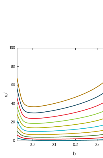
Figure 4: The eigenvalues of ten lowest even-parity perturbations of the $R^{2}$ EYM solutions are shown as functions of the parameter $b$ for $\kappa=1$ and $R=-1$.

V Conclusions

The objective of this work was to investigate properties of new regular solutions of the $\mbox{SU}(2)$ Yang-Mills theory, coupled to the pure $R^{2}$ gravity. We found a family of non-trivial spherically symmetrical solutions with non-vanishing magnetic charge, which generalize the usual Bartnik-McKinnon solitons in the EYM theory. We found that the $R^{2}$ EYM model has only solutions with no node in the gauge field profile function, or with a single node, there is no solutions with multiple nodes. Similar to the BM solutions in asymptotically AdS₄ spacetime, the nodeless solutions are stable with respect to linear perturbations.

We remark that the scale invariant $R^{2}$ EYM model is very different from the generalizations of gravity, which also include the usual linear in curvature term. The $R+R^{2}$ model is also ghost-free, however it is equivalent to the conventional Einstein gravity with an additional scalar field. Further, we found that such a model supports only regular solutions, for which the curvature scalar is zero and $T_{\mu\nu}=0$.

The scale invariance of the $R^{2}$ model with the non-Abelian matter fields will be broken when the $R^{2}$ gravity will be coupled to the Yang-Mills-Higgs system with symmetry breaking potential. We expect the properties of the corresponding monopole solutions will be different from the standard gravitating monopoles in asymptotically AdS₄ spacetime. Another direction for further work is to investigate $R^{2}$ EYM non-Abelian configurations with both electric and magnetic charges.

References

- (1) A. A. Starobinsky, Phys. Lett. 91B (1980) 99.
- (2) A. Salam and J. A. Strathdee, Phys. Rev. D 18 (1978) 4480.
- (3) K. S. Stelle, Phys. Rev. D 16 (1977) 953.
- (4) K. S. Stelle, Gen. Rel. Grav. 9 (1978) 353.
- (5) S. Capozziello, Int. J. Mod. Phys. D 11 (2002) 483
- (6) A. A. Starobinsky, JETP Lett. 86 (2007) 157
- (7) C. Kounnas, D. Lüst and N. Toumbas, Fortsch. Phys. 63 (2015) 12
- (8) J. Ellis, D. V. Nanopoulos and K. A. Olive, Phys. Rev. Lett. 111 (2013) 111301 Erratum: [Phys. Rev. Lett. 111 (2013) no.12, 129902]
- (9) S. Ferrara, A. Kehagias and M. Porrati, JHEP 1508 (2015) 001
- (10) L. Alvarez-Gaume, A. Kehagias, C. Kounnas, D. Lüst and A. Riotto, Fortsch. Phys. 64 (2016) no.2-3, 176
- (11) S. M. Kuzenko, Phys. Rev. D 94 (2016) no.6, 065014
- (12) A. Kehagias, C. Kounnas, D. Lüst and A. Riotto, JHEP 1505 (2015) 143
- (13) F. Duplessis and D. A. Easson, Phys. Rev. D 92 (2015) no.4, 043516
- (14) J. Ellis, D. V. Nanopoulos and K. A. Olive, arXiv:1711.11051 [hep-th].
- (15) R. Bartnik and J. Mckinnon, Phys. Rev. Lett. 61 (1988) 141.
- (16) M. S. Volkov and D. V. Galtsov, JETP Lett. 50 (1989) 346 [Pisma Zh. Eksp. Teor. Fiz. 50 (1989) 312]
- (17) P. Bizon, Phys. Rev. Lett. 64 (1990) 2844.
- (18) G. V. Lavrelashvili and D. Maison, Nucl. Phys. B 410 (1993) 407
- (19) M. S. Volkov and D. V. Gal’tsov, Phys. Rept. 319, 1 (1999)
- (20) M. S. Volkov, arXiv:1601.08230 [gr-qc].
- (21) D. V. Galtsov and A. A. Ershov, Phys. Lett. A 138 (1989) 160.
- (22) P. Bizon and O. T. Popp, Class. Quant. Grav. 9 (1992) 193.
- (23) N. Straumann and Z. H. Zhou, Phys. Lett. B 237 (1990) 353.
- (24) Z. h. Zhou and N. Straumann, Nucl. Phys. B 360 (1991) 180.
- (25) H. P. Kuenzle, Class. Quant. Grav. 8 (1991) 2283.
- (26) B. Kleihaus, J. Kunz and A. Sood, Phys. Lett. B 354 (1995) 240
- (27) R. A. Bartnik, M. Fisher and T. A. Oliynyk, J. Math. Phys. 51 (2010) 032504
- (28) T. A. Oliynyk and H. P. Kunzle, J. Math. Phys. 43 (2002) 2363
- (29) G. V. Lavrelashvili and D. Maison, Phys. Lett. B 343 (1995) 214
- (30) B. Kleihaus and J. Kunz, Phys. Rev. Lett. 78 (1997) 2527
- (31) O. Brodbeck and N. Straumann, Phys. Lett. B 324 (1994) 309
- (32) R. Ibadov, B. Kleihaus, J. Kunz and Y. Shnir, Phys. Lett. B 609 (2005) 150
- (33) E. Winstanley, Class. Quant. Grav. 16 (1999) 1963
- (34) J. Bjoraker and Y. Hosotani, Phys. Rev. Lett. 84 (2000) 1853
- (35) J. Bjoraker and Y. Hosotani, Phys. Rev. D 62 (2000) 043513
- (36) E. Radu and D. H. Tchrakian, Class. Quant. Grav. 22 (2005) 879
- (37) D. Sudarsky and R. M. Wald, Phys. Rev. D 46 (1992) 1453.
- (38) O. Sarbach and E. Winstanley, Class. Quant. Grav. 18 (2001) 2125
- (39) J. E. Baxter, M. Helbling and E. Winstanley, Phys. Rev. D 76 (2007) 104017
- (40) E. Winstanley, Lect. Notes Phys. 769 (2009) 49
- (41) E. Radu, Phys. Rev. D 65 (2002) 044005
- (42) O. Kichakova, J. Kunz, E. Radu and Y. Shnir, Phys. Rev. D 90 (2014) no.12, 124012
- (43) S. S. Gubser and S. S. Pufu, JHEP 0811 (2008) 033
- (44) M. S. Volkov, N. Straumann, G. V. Lavrelashvili, M. Heusler and O. Brodbeck, Phys. Rev. D 54 (1996) 7243
- (45) S. Deser and B. Tekin, Phys. Rev. Lett. 89 (2002) 101101
- (46) S. Deser and B. Tekin, Phys. Rev. D 75 (2007) 084032