On $\mathcal{L}_{\infty}$ string stability of nonlinear bidirectional asymmetric heterogeneous platoon systems

Julien Monteil    Giovanni Russo giovanni.russo1@ucd.ie    Robert Shorten IBM Research - Ireland Lab. Address: IBM Technology Campus, Mulhuddart, Dublin, 15. University College Dublin, School of Electrical Engineering. Address: Belfield, Dublin, $4$.
Abstract

This paper is concerned with the study of bidirectionally coupled platoon systems. The case considered is when the vehicles are heterogeneous and the coupling can be nonlinear and asymmetric. For such systems, a sufficient condition for $\mathcal{L}_{\infty}$ string stability is presented. The effectiveness of our approach is illustrated via a numerical example, where it is shown how our result can be recast as an optimization problem, allowing to design the control protocol for each vehicle independently on the other vehicles and hence leading to a bottom-up approach for the design of string stable systems able to track a time-varying reference speed.

keywords:
Vehicular platoons, Multi-Vehicle Systems, String Stability, Asymmetric Coupling

1 Introduction

Platoon systems designate a class of network systems where automated vehicles, typically arranged in a string, cooperate via some distributed control protocol, or coupling, in order to travel along the longitudinal direction (Levine and Athans, 1966). The vehicles need to attain a configuration where a common driving speed is achieved and, at the same time, some desired vehicle-to-vehicle distance is kept. Typically, the distributed protocols needs to be designed so as to ensure string stability of the platoon system, see e.g. (Seiler et al., 2004; Middleton and Braslavsky, 2010; Barooah et al., 2009; Hao et al., 2011; Zheng et al., 2016). Intuitively, if the system is string stable, then: (i) vehicles can attain and keep the desired configuration; (ii) the effects of disturbances are attenuated along the string.

A platoon system is said to be unidirectional (also termed as leader-follower topology) if the control protocol on each vehicle only takes as input information coming from the vehicles ahead, while it is said to be bidirectional if the control protocol takes as input information coming from the vehicles ahead and behind, see e.g. (Middleton and Braslavsky, 2010; Nieuwenhuijze, 2010). Recently, see e.g. (Hao et al., 2012; Martinec et al., 2016; Herman et al., 2017a, b), asymmetric bidirectional control algorithms have been considered, where the information from the vehicles ahead might be weighted differently than the information from the vehicles behind. Also, the platoon system is said to be homogeneous if the vehicles are all identical, heterogeneous otherwise.

Literature review

Historically, work on string stability can be traced back to (Peppard, 1974) and to the California PATH program, see e.g. (Sheikholeslam and Desoer, 1990). A convenient way to formalize the concept of string stability is via the use of $p$-signal norms. The concept of $\mathcal{L}_{p}$ string stability has been originally introduced in (Swaroop and Hedrick, 1996), where a number of sufficient conditions ensuring this property were also given. In such a paper, $\mathcal{L}_{p}$ string stability was defined for interconnected systems with no external disturbance. Recently, a similar formalism has been used in (Knorn et al., 2014), where $\mathcal{L}_{p}$ string stability has been defined for systems affected by external disturbances. Another convenient way to formalize $\mathcal{L}_{p}$ string stability has been introduced in (Ploeg et al., 2014b). In such a paper, the definition of string stability is given for systems where the first vehicle is affected by an external disturbance imposed by the leading vehicle. Essentially, following (Ploeg et al., 2014b), the platoon system with the first vehicle affected by the disturbance is $\mathcal{L}_{p}$ string stable if the $\mathcal{L}_{p}$ signal norm of the local error vector between the current and target states of the system is upper bounded by certain class $\mathcal{K}$ functions.

The notions of $\mathcal{L}_{2}$ and $\mathcal{L}_{\infty}$ string stability are particularly useful for applications. As noted in (Ploeg et al., 2014b), the use of $\mathcal{L}_{2}$ string stability is motivated by requirements of energy dissipation along the system, while the notion of $\mathcal{L}_{\infty}$ string stability is related to the maximum vehicle overshoot (Stuedli et al., 2017). This concept, in turn, has a direct interpretation in terms of vehicle collisions. For linear systems, studying $\mathcal{L}_{2}$ string stability, while lacking the interpretation in terms of collision avoidance, is analytically convenient as results can be stated in terms of the $\mathcal{H}_{\infty}$ system norm of the transfer function.

In (Middleton and Braslavsky, 2010) it is shown how $\mathcal{L}_{2}$ string stability can be achieved for a linear platoon by allowing inter-vehicle communications and in (Ploeg et al., 2014a), the design of a $\mathcal{L}_{2}$ string stable cooperative adaptive cruise controller, making use of a feed-forward term, is presented for linear systems where the disturbance is on the first vehicle. In the linear setting, in (Nieuwenhuijze, 2010) a $\mathcal{L}_{2}$ string stability definition in the $z$-domain is given for homogeneous platoon systems and this is used to analyze the performance of bidirectional constant time headway control policies. In particular, one of the main findings is that the use of a bidirectional structure can result in a better disturbance attenuation when compared to a predecessor-follower strategy. Recently, in (Swaroop and Rajagopal, 2001; Swaroop et al., 2017), it has been shown that constant time-headway policies can be used to enhance $\mathcal{L}_{2}$ string stability in linear platoon systems. Also, in (Hao et al., 2012), the robustness to external disturbances is investigated for linear, heterogeneous, platoon systems where vehicles are modeled as double integrators and where the disturbance is a sinusoidal function. In particular, quantitative comparisons between unidirectional, bidirectional and asymmetric bidirectional control protocols are presented in the paper and it is shown how asymmetric bidirectional control protocols can have a beneficial effect on string stability. Indeed, one of the main findings of this paper is that asymmetric weights on the velocity feedback enhances robustness of the platoon system. The implications of asymmetric bidirectional control protocols on disturbance scaling and $\mathcal{L}_{2}$ string stability have been further investigated for linear platoons in (Herman et al., 2017a), and in (Martinec et al., 2016) via a wave-based control approach. In (Yanakiev and Kanellakopoulos, 1998), nonlinear spacing policies are introduced for automated heavy-duty vehicles and string stability is proven on the linearized system. Instead, an approach to the design of nonlinear protocols for platoon systems has been presented in (Knorn et al., 2014), where energy-based arguments are used to prove $\mathcal{L}_{2}$ string stability. This approach has been also expanded in (Knorn et al., 2015) to mitigate the effects of time-varying measurement errors on the platoon. Finally, in (Monteil and Russo, 2017), nonlinear control protocols are studied but only stability is considered rather than string stability, while consensus-based approaches are explored in (di Bernardo et al., 2015) and (Zegers et al., 2017), where exponential stability is considered in the case where some of the vehicles in the platoon are subject to speed restrictions.

The literature on $\mathcal{L}_{\infty}$ string stability of linear platoon systems is sparse when compared to the literature on $\mathcal{L}_{2}$ string stability. Conditions for $\mathcal{L}_{\infty}$ string stability of linear, unidirectional, platoon systems have been originally investigated in (Swaroop and Hedrick, 1996, Chapter $5$). Other works on $\mathcal{L}_{\infty}$ string stability of linear platoon systems include (Swaroop and Hedrick, 1999; de Wit and Brogliato, 1999; Rogge and Aeyels, 2008; Monteil et al., 2018). In particular, in (Swaroop and Hedrick, 1999; de Wit and Brogliato, 1999) unidirectional platoons with no external disturbances are considered, while in (Rogge and Aeyels, 2008) the platoon does not have a leading vehicle and the use of ring interconnection topologies are explored, when only the first vehicle is affected by an external disturbance. Finally, in the recent work (Besselink and Johansson, 2017), the problem of studying $\mathcal{L}_{\infty}$ string stability for nonlinear homogeneous, unidirectional, platoons is investigated in the spatial domain and the methodology is illustrated by designing distributed protocols requiring each vehicle to use position, speed and acceleration from the leading vehicle.

Contribution of this paper

In the context of the above literature, this paper offers the following contributions: (i) a novel sufficient condition for $\mathcal{L}_{\infty}$ string stability is presented for heterogeneous platoon systems coupled with nonlinear, asymmetric bidirectional control protocols and subject to disturbances. The string stability definition used in this paper generalizes a number of definitions commonly used in the literature (see Definition 1 and Remark 1); (ii) The control policies devised following our theoretical results allow the platoon system to track a desired (possibly, non-constant) reference speed: this is particularly appealing for applications, where the reference speed might be used to e.g. set speed restrictions; (iii) It is shown how our theoretical results can be effectively used to design protocols guaranteeing $\mathcal{L}_{\infty}$ string stability of the platoon system. Namely, we show how the results can be recast as an optimization problem that allows to design the control protocol for each vehicle independently on the other vehicles.

2 Notation and problem formulation

2.1 Notation

Let $v$ be an arbitrary $m$-dimensional vector, $A$ be a $m\times m$ matrix and $\Theta$ be a non-singular $m\times m$ matrix. By $\left|v\right|_{p}$ we denote an arbitrary $p$-vector norm on ${\mathbb{R}}^{m}$, while $\left\|A\right\|_{p}$ and $\mu_{p}(A)$ denote the matrix norm and matrix measure of $A$ induced by $\left|\cdot\right|_{p}$, see e.g. (Vidyasagar, 1993) and Appendix A. Then, $\left|v\right|_{\Theta,p}=\left|\Theta v\right|_{p}$ is also a vector norm and its induced matrix measure is equal to $\mu_{\Theta,p}(A)=\mu_{p}\left(\Theta A\Theta^{-1}\right)$. We also denote by $\sigma_{\max}(A)$ ($\sigma_{\min}(A)$) the largest (smallest) singular value of $A$, by $[A]_{s}$ the symmetric part of $A$ and by $I_{m}$ the identity matrix of dimension $m$. The notation $A\succeq 0$ indicates that the matrix $A$ is positive semi-definite and $A\prec B$ that the matrix $A-B$ is negative definite. Consider the signal $d(\cdot):{\mathbb{R}}_{+}\rightarrow\mathcal{D}\subseteq{\mathbb{R}}^{n}$. Then, the supremum norm of $d(\cdot)$ is denoted by $\left\|d(\cdot)\right\|_{\mathcal{L}_{\infty}}=\sup_{t\geq 0}\left|d(t)\right|_{2}$. A continuous function, $a(\cdot):{\mathbb{R}}_{+}\rightarrow{\mathbb{R}}_{+}$ is: (i) a class-$\mathcal{K}$ function if $a(0)=0$ and $a(\cdot)$ is strictly increasing; (ii) a class-$\mathcal{L}$ function if it monotonically decreases to 00 as its argument tends to $+\infty$. A continuous function, $b(\cdot,\cdot):{\mathbb{R}}_{+}\times{\mathbb{R}}_{+}\rightarrow{\mathbb{R}}_{+}$, is a class-$\mathcal{KL}$ function if $b(\cdot,t)$ is a class-$\mathcal{K}$ function $\forall t\geq 0$ and $b(\xi,\cdot)$ is a class-$\mathcal{L}$ function, $\forall\xi\geq 0$.

2.2 System description

We consider platoon systems of $N>1$ heterogeneous vehicles arranged along a string and following a leading vehicle (vehicle 00). The dynamics of the $i$-th vehicle within the platoon is governed by:

$$\dot{x}_{i}=f_{i}(x_{i})+\tilde{u}_{i}+d_{i},\ \ \ x_{i}(t_{0})=x_{i,0},\ \ \ t_{0}\geq 0,$$ (1)

$i=1,\dots,N$. We consider the case where: (i) $x_{i}\in{\mathbb{R}}^{n}$; (ii) $f_{i}(x_{i}):{\mathbb{R}}^{n}\rightarrow{\mathbb{R}}^{n}$ are smooth functions; (iii) $\tilde{u}_{i}(t)$ is the distributed control protocol having the form

u~i(t):=h~i,i1(t,xi1,xi)+εih~i,i+1(t,xi+1,xi)+h~i(0)(t,xi,x0).assignsubscript~𝑢𝑖𝑡subscript~𝑖𝑖1𝑡subscript𝑥𝑖1subscript𝑥𝑖subscript𝜀𝑖subscript~𝑖𝑖1𝑡subscript𝑥𝑖1subscript𝑥𝑖superscriptsubscript~𝑖0𝑡subscript𝑥𝑖subscript𝑥0\begin{split}\tilde{u}_{i}(t)&:=\tilde{h}_{i,i-1}(t,x_{i-1},x_{i})+\varepsilon_{i}\tilde{h}_{i,i+1}(t,x_{i+1},x_{i})\\ &+{\color[rgb]{0,0,0}\definecolor[named]{pgfstrokecolor}{rgb}{0,0,0}\pgfsys@color@gray@stroke{0}\pgfsys@color@gray@fill{0}\tilde{h}_{i}^{(0)}}(t,x_{i},x_{0}).\end{split} (2)

In (2) the functions $\tilde{h}_{ij}:{\mathbb{R}}_{+}\times{\mathbb{R}}^{n}\times{\mathbb{R}}^{n}\rightarrow{\mathbb{R}}^{n}$ are smooth coupling functions and $0\leq\varepsilon_{i}\leq 1$ is the coupling gain between vehicle $i$ and the vehicle behind, i.e. vehicle $i+1$(Herman et al., 2017a). We say that (2) is: (i) an asymmetric control protocol, if $0<\varepsilon_{i}<1$; (ii) a predecessor-follower protocol, if $\varepsilon_{i}=0$; (iii) a bidirectional protocol, if $\varepsilon_{i}=1$. In (2), $x_{0}$ is the input received from vehicle 00 and the smooth function h~i(0)(,)superscriptsubscript~𝑖0{\color[rgb]{0,0,0}\definecolor[named]{pgfstrokecolor}{rgb}{0,0,0}\pgfsys@color@gray@stroke{0}\pgfsys@color@gray@fill{0}\tilde{h}_{i}^{(0)}}(\cdot,\cdot) represents a direct coupling, which requires a communication infrastructure, from the leading vehicle to vehicle $i$. If there is no communication between those vehicles, then h~i(0)(,)=0superscriptsubscript~𝑖00{\color[rgb]{0,0,0}\definecolor[named]{pgfstrokecolor}{rgb}{0,0,0}\pgfsys@color@gray@stroke{0}\pgfsys@color@gray@fill{0}\tilde{h}_{i}^{(0)}}(\cdot,\cdot)=0 by definition. The dynamics (1) - (2) models a network of nonlinear heterogeneous vehicles coupled via time-dependent coupling functions. Explicitly including nonlinearities in the design of the control protocols is useful in certain applications such as platooning of heavy-duty vehicles where the nonlinearities at the vehicles cannot be neglected, see e.g. (Alam et al., 2015) and references therein. Finally, $d_{i}(t)$ is an $n$-dimensional disturbance acting on the $i$-th vehicle (in the context of this paper a disturbance is an $n$-dimensional signal with all of its components being piece-wise continuous), $d(t):=[d_{1}(t)^{T},\ldots,d_{N}(t)^{T}]^{T}$ and $X(t):=[x_{1}(t)^{T},\ldots,x_{N}(t)^{T}]^{T}$.

2.3 Control goals

In order to introduce our results we define the unperturbed dynamics of (1) - (2) as

y˙i=fi(yi)+h~i,i1(t,yi1,yi)+εih~i,i+1(t,yi+1,yi)+h~i(0)(t,yi,x0),subscript˙𝑦𝑖subscript𝑓𝑖subscript𝑦𝑖subscript~𝑖𝑖1𝑡subscript𝑦𝑖1subscript𝑦𝑖subscript𝜀𝑖subscript~𝑖𝑖1𝑡subscript𝑦𝑖1subscript𝑦𝑖superscriptsubscript~𝑖0𝑡subscript𝑦𝑖subscript𝑥0\begin{split}\dot{y}_{i}&=f_{i}(y_{i})+\tilde{h}_{i,i-1}(t,y_{i-1},y_{i})\\ &+\varepsilon_{i}\tilde{h}_{i,i+1}(t,y_{i+1},y_{i})+{\color[rgb]{0,0,0}\definecolor[named]{pgfstrokecolor}{rgb}{0,0,0}\pgfsys@color@gray@stroke{0}\pgfsys@color@gray@fill{0}\tilde{h}_{i}^{(0)}}(t,y_{i},x_{0}),\end{split} (3)

and we denote by $Y(t):=[y_{1}(t)^{T},\ldots,y_{N}(t)^{T}]^{T}$ the stack of all $y_{i}$’s. Also, the desired solution for (3) is denoted by $Y^{\ast}(t):=[y_{1}^{\ast}(t)^{T},\ldots,\break y_{N}^{\ast}(t)^{T}]^{T}$, with $\dot{y}^{\ast}_{i}=f_{i}(y^{\ast}_{i})$, $\forall i=1,\ldots,N$. That is, $Y^{\ast}(t)$ corresponds to a desired configuration of the platoon system when there are no disturbances. Our goal in this paper is to design the control protocols $\tilde{u}_{i}(\cdot)$ in (1) so as to guarantee disturbance $\mathcal{L}_{\infty}$ string stability of the platoon system. This is formalized via the following definition, see also (Besselink and Johansson, 2017)

Definition 1.

Consider the platoon system (1) and assume that $Y^{\ast}(t)$ is a solution of its unperturbed dynamics (3). Then, (1) is said to be disturbance $\mathcal{L}_{\infty}$ string stable if there exists a class $\mathcal{KL}$ function, $\alpha$, a class-$\mathcal{K}$ function, $\beta$, such that, for any disturbance $d(t)$ and initial conditions, we have, $\forall t\geq t_{0}$, supi|xi(t)yi(t)|2α(supi|xi(t0)yi(t0)|2,t)+β(supidi())subscriptsupremum𝑖subscriptsubscript𝑥𝑖𝑡superscriptsubscript𝑦𝑖𝑡2𝛼subscriptsupremum𝑖subscriptsubscript𝑥𝑖subscript𝑡0superscriptsubscript𝑦𝑖subscript𝑡02𝑡𝛽subscriptsupremum𝑖subscriptnormsubscript𝑑𝑖subscript{\color[rgb]{0,0,0}\definecolor[named]{pgfstrokecolor}{rgb}{0,0,0}\pgfsys@color@gray@stroke{0}\pgfsys@color@gray@fill{0}{\sup_{i}\left|x_{i}(t)-y_{i}^{\ast}(t)\right|}_{{\color[rgb]{0,0,0}\definecolor[named]{pgfstrokecolor}{rgb}{0,0,0}\pgfsys@color@gray@stroke{0}\pgfsys@color@gray@fill{0}2}}}\leq\alpha\left({\color[rgb]{0,0,0}\definecolor[named]{pgfstrokecolor}{rgb}{0,0,0}\pgfsys@color@gray@stroke{0}\pgfsys@color@gray@fill{0}\sup_{i}\left|x_{i}(t_{0})-y_{i}^{\ast}(t_{0})\right|_{2}},t\right)+\beta\left({\color[rgb]{0,0,0}\definecolor[named]{pgfstrokecolor}{rgb}{0,0,0}\pgfsys@color@gray@stroke{0}\pgfsys@color@gray@fill{0}\sup_{i}}\left\|d_{{\color[rgb]{0,0,0}\definecolor[named]{pgfstrokecolor}{rgb}{0,0,0}\pgfsys@color@gray@stroke{0}\pgfsys@color@gray@fill{0}i}}(\cdot)\right\|_{\mathcal{L}_{\infty}}\right).

Remark 1.

In the above definition, supi|xi(t)yi(t)|2subscriptsupremum𝑖subscriptsubscript𝑥𝑖𝑡superscriptsubscript𝑦𝑖𝑡2{\color[rgb]{0,0,0}\definecolor[named]{pgfstrokecolor}{rgb}{0,0,0}\pgfsys@color@gray@stroke{0}\pgfsys@color@gray@fill{0}{\sup_{i}\left|x_{i}(t)-y_{i}^{\ast}(t)\right|}_{{\color[rgb]{0,0,0}\definecolor[named]{pgfstrokecolor}{rgb}{0,0,0}\pgfsys@color@gray@stroke{0}\pgfsys@color@gray@fill{0}2}}} is upper bounded by the same functions $\alpha(\cdot,\cdot)$ and $\beta(\cdot)$ for any platoon length, $N$. That is, the bounds of the definition are independent on the number of vehicles. Definition 1 is stated via the input-to-state stability formalism, see e.g. (Sontag, 2008; Khalil, 2002), and disturbances are explicitly considered (in the definition given in e.g. (Swaroop and Hedrick, 1996) disturbances are not considered). Also, Definition 1 generalizes the definition given in (Ploeg et al., 2014a) as it allows to consider platoon systems with disturbances acting on any vehicle within the system.

Remark 2.

Definition 1 can be equivalently stated in terms of $\left|\cdot\right|_{\infty}$ by noticing that:

supi|xi(t)yi(t)|2supi|xi(t)yi(t)|supi|xi(0)yi(0)|2nsupi|xi(0)yi(0)|di()nsupisupt|di(t)|,subscriptsupremum𝑖subscriptsubscript𝑥𝑖𝑡superscriptsubscript𝑦𝑖𝑡2subscriptsupremum𝑖subscriptsubscript𝑥𝑖𝑡superscriptsubscript𝑦𝑖𝑡subscriptsupremum𝑖subscriptsubscript𝑥𝑖0superscriptsubscript𝑦𝑖02𝑛subscriptsupremum𝑖subscriptsubscript𝑥𝑖0superscriptsubscript𝑦𝑖0subscriptdelimited-∥∥subscript𝑑𝑖subscript𝑛subscriptsupremum𝑖subscriptsupremum𝑡subscriptsubscript𝑑𝑖𝑡\begin{split}\sup_{i}\left|x_{i}(t)-y_{i}^{\ast}(t)\right|_{2}&\geq\sup_{i}\left|x_{i}(t)-y_{i}^{\ast}(t)\right|_{{\color[rgb]{0,0,0}\definecolor[named]{pgfstrokecolor}{rgb}{0,0,0}\pgfsys@color@gray@stroke{0}\pgfsys@color@gray@fill{0}\infty}}\\ \sup_{i}\left|x_{i}(0)-y_{i}^{\ast}(0)\right|_{2}&\leq\sqrt{n}\sup_{i}\left|x_{i}(0)-y_{i}^{\ast}(0)\right|_{\infty}\\ \left\|d_{i}(\cdot)\right\|_{\mathcal{L}_{\infty}}&\leq\sqrt{n}\sup_{i}\sup_{t}\left|d_{i}(t)\right|_{\infty},\end{split}

thus giving a bound that is still independent on the number of vehicles, $N$.

In what follows, systems fulfilling Definition 1 are simply termed as $\mathcal{L}_{\infty}$ string stable. Finally, we now establish a link between Definition 1 and the string stability definition given in (Swaroop and Hedrick, 1996).

Lemma 1.

Assume that the platoon system (1) is $\mathcal{L}_{\infty}$ string stable in accordance to Definition 1. Then, if $d_{i}(t)=0$, $\forall t\geq 0$ and $\forall i=1,\ldots,N$, Definition 1 is equivalent to the definition given in (Swaroop and Hedrick, 1996).

Proof. The proof can be obtained from (Khalil, 2002, page $175$) and it is omitted here for brevity. ∎

3 Results

With the result below, a sufficient condition for $\mathcal{L}_{\infty}$ string stability of the platoon system is given.

Theorem 1.

Consider the platoon system (1) controlled by the distributed control strategy (2). Assume that the coupling functions $\tilde{h}_{i,i-1}$, $\tilde{h}_{i,i+1}$, h~i(0)superscriptsubscript~𝑖0{\color[rgb]{0,0,0}\definecolor[named]{pgfstrokecolor}{rgb}{0,0,0}\pgfsys@color@gray@stroke{0}\pgfsys@color@gray@fill{0}\tilde{h}_{i}^{(0)}} and the control gains $\varepsilon_{i}$ are designed in a way such that, $\forall i=1,\ldots,N$ and $\forall t\geq t_{0}$:

  1. C1 -

    $\tilde{h}_{i,i-1}\left(t,y^{\ast}_{i-1},y^{\ast}_{i}\right)=\tilde{h}_{i,i+1}\left(t,y^{\ast}_{i+1},y^{\ast}_{i}\right)=0$, hi(0)(t,yi,x0)=0superscriptsubscript𝑖0𝑡subscriptsuperscript𝑦𝑖subscript𝑥00{\color[rgb]{0,0,0}\definecolor[named]{pgfstrokecolor}{rgb}{0,0,0}\pgfsys@color@gray@stroke{0}\pgfsys@color@gray@fill{0}h_{i}^{(0)}}\left(t,y^{\ast}_{i},x_{0}\right)=0;

  2. C2 -

    for some $c\neq 0$, $\bar{J}>0$

    μ2(fxi+h~i(0)xi+h~i,i1xi+εih~i,i+1xi)c2,max{h~i,i1xi12,h~i,i+1xi+12}J¯,formulae-sequencesubscript𝜇2𝑓subscript𝑥𝑖superscriptsubscript~𝑖0subscript𝑥𝑖subscript~𝑖𝑖1subscript𝑥𝑖subscript𝜀𝑖subscript~𝑖𝑖1subscript𝑥𝑖superscript𝑐2subscriptdelimited-∥∥subscript~𝑖𝑖1subscript𝑥𝑖12subscriptdelimited-∥∥subscript~𝑖𝑖1subscript𝑥𝑖12¯𝐽\begin{split}&\mu_{2}\left(\frac{\partial f}{\partial x_{i}}+\frac{\partial{\color[rgb]{0,0,0}\definecolor[named]{pgfstrokecolor}{rgb}{0,0,0}\pgfsys@color@gray@stroke{0}\pgfsys@color@gray@fill{0}\tilde{h}_{i}^{(0)}}}{\partial x_{i}}+\frac{\partial\tilde{h}_{i,i-1}}{\partial x_{i}}+\varepsilon_{i}\frac{\partial\tilde{h}_{i,i+1}}{\partial x_{i}}\right)\leq-c^{2},\\ &\max\left\{\left\|\frac{\partial\tilde{h}_{i,i-1}}{\partial x_{i-1}}\right\|_{2},\left\|\frac{\partial\tilde{h}_{i,i+1}}{\partial x_{i+1}}\right\|_{2}\right\}\leq\bar{J},\end{split} (4)

    $\forall x_{i},x_{i-1},x_{i+1}\in{\mathbb{R}}^{n}$;

  3. C3 -

    $\varepsilon_{i}<\frac{c^{2}}{\bar{J}}-1$.

Then,

supi|xi(t)yi(t)|2ec¯2(tt0)supi|xi(t0)yi(t0)|2+1ec¯2(tt0)c¯2supidi(),subscriptsupremum𝑖subscriptsubscript𝑥𝑖𝑡superscriptsubscript𝑦𝑖𝑡2superscript𝑒superscript¯𝑐2𝑡subscript𝑡0subscriptsupremum𝑖subscriptsubscript𝑥𝑖subscript𝑡0superscriptsubscript𝑦𝑖subscript𝑡021superscript𝑒superscript¯𝑐2𝑡subscript𝑡0superscript¯𝑐2subscriptsupremum𝑖subscriptdelimited-∥∥subscript𝑑𝑖subscript\begin{split}\sup_{i}\left|x_{i}(t)-y_{i}^{\ast}(t)\right|_{{\color[rgb]{0,0,0}\definecolor[named]{pgfstrokecolor}{rgb}{0,0,0}\pgfsys@color@gray@stroke{0}\pgfsys@color@gray@fill{0}2}}&\leq e^{-\bar{c}^{2}(t-t_{0})}\sup_{i}\left|x_{i}(t_{0})-y_{i}^{\ast}(t_{0})\right|_{{\color[rgb]{0,0,0}\definecolor[named]{pgfstrokecolor}{rgb}{0,0,0}\pgfsys@color@gray@stroke{0}\pgfsys@color@gray@fill{0}2}}\\ &+\frac{1-e^{-\bar{c}^{2}(t-t_{0})}}{\bar{c}^{2}}{\color[rgb]{0,0,0}\definecolor[named]{pgfstrokecolor}{rgb}{0,0,0}\pgfsys@color@gray@stroke{0}\pgfsys@color@gray@fill{0}\sup_{i}\left\|d_{i}(\cdot)\right\|_{\mathcal{L}_{\infty}}},\end{split}

$\forall t\geq t_{0}$, where $\bar{c}^{2}:=c^{2}-\bar{J}(1+\max_{i}\varepsilon_{i})$.

Proof. See Appendix B. ∎

We now focus on the special case where: (i) the vehicles within the platoon in (1) are modeled via a second order linear system with a disturbance acting on the acceleration; (ii) the desired platoon configuration is the configuration where vehicles keep a desired distance from the vehicle ahead, while following a reference speed. In doing so, we denote by qi(t)subscript𝑞𝑖𝑡{\color[rgb]{0,0,0}\definecolor[named]{pgfstrokecolor}{rgb}{0,0,0}\pgfsys@color@gray@stroke{0}\pgfsys@color@gray@fill{0}q_{i}}(t) and $v_{i}(t)$ the position and speed of the $i$-th vehicle (xi(t):=[qi(t),vi(t)]Tassignsubscript𝑥𝑖𝑡superscriptsubscript𝑞𝑖𝑡subscript𝑣𝑖𝑡𝑇x_{i}(t):=[{\color[rgb]{0,0,0}\definecolor[named]{pgfstrokecolor}{rgb}{0,0,0}\pgfsys@color@gray@stroke{0}\pgfsys@color@gray@fill{0}q_{i}}(t),v_{i}(t)]^{T}) having as initial conditions qi(0)subscript𝑞𝑖0{\color[rgb]{0,0,0}\definecolor[named]{pgfstrokecolor}{rgb}{0,0,0}\pgfsys@color@gray@stroke{0}\pgfsys@color@gray@fill{0}q_{i}}(0) and $v_{i}(0)$. The (possibly) time-varying reference speed is v0(t)subscript𝑣0𝑡v_{0}{\color[rgb]{0,0,0}\definecolor[named]{pgfstrokecolor}{rgb}{0,0,0}\pgfsys@color@gray@stroke{0}\pgfsys@color@gray@fill{0}(t)} and, without loss of generality we assume that $q_{0}(0)=0$. Then, the position of the leading vehicle at time $t$ is denoted by $q_{0}(t)$ and we let x0(t):=[q0(t),v0(t)]Tassignsubscript𝑥0𝑡superscriptsubscript𝑞0𝑡subscript𝑣0𝑡𝑇x_{0}(t):=[q_{0}(t),v_{0}{\color[rgb]{0,0,0}\definecolor[named]{pgfstrokecolor}{rgb}{0,0,0}\pgfsys@color@gray@stroke{0}\pgfsys@color@gray@fill{0}(t)}]^{T} be the input from the leading vehicle to the platoon system. The dynamics of the $i$-th vehicle, $i=1,\ldots,N$, is governed by:

qi˙=vi,miv˙i=u¯i+d¯i,formulae-sequence˙subscript𝑞𝑖subscript𝑣𝑖subscript𝑚𝑖subscript˙𝑣𝑖subscript¯𝑢𝑖subscript¯𝑑𝑖\begin{split}&\dot{{\color[rgb]{0,0,0}\definecolor[named]{pgfstrokecolor}{rgb}{0,0,0}\pgfsys@color@gray@stroke{0}\pgfsys@color@gray@fill{0}q_{i}}}=v_{i},\\ &m_{i}\dot{v}_{i}=\bar{u}_{i}+\bar{d}_{i},\end{split}

where $m_{i}$ is the mass of the $i$-th vehicle in the system, $\bar{d}_{i}(t)$ is a one-dimensional time-dependent disturbance on the vehicle and $\bar{u}_{i}(t)$ is the decentralized control protocol for the $i$-th vehicle. In compact form we have:

$$\begin{split}\dot{x}_{i}&=Fx_{i}+u_{i}+d_{i},\end{split}$$ (5)

$i=1,\ldots,N$ and where: (i) $d_{i}(t):=1/m_{i}[0,\bar{d}_{i}(t)]^{T}$; (ii) $F=\begin{bmatrix}0&1\\ 0&0\end{bmatrix}$; (iii) $u_{i}(t)=[0,\bar{u}_{i}(t)]^{T}$. For notational convenience, we let

1miu¯i(t):=hi,i1(xi1,xi)+εihi,i+1(xi+1,xi)+hi(0)(xi,x0),i=1,N.formulae-sequenceassign1subscript𝑚𝑖subscript¯𝑢𝑖𝑡subscript𝑖𝑖1subscript𝑥𝑖1subscript𝑥𝑖subscript𝜀𝑖subscript𝑖𝑖1subscript𝑥𝑖1subscript𝑥𝑖superscriptsubscript𝑖0subscript𝑥𝑖subscript𝑥0for-all𝑖1𝑁\begin{split}\frac{1}{m_{i}}\bar{u}_{i}(t):=&h_{i,i-1}(x_{i-1},x_{i})+\varepsilon_{i}h_{i,i+1}(x_{i+1},x_{i})\\ &+{\color[rgb]{0,0,0}\definecolor[named]{pgfstrokecolor}{rgb}{0,0,0}\pgfsys@color@gray@stroke{0}\pgfsys@color@gray@fill{0}h_{i}^{(0)}}(x_{i},x_{0}),\ \forall i=1,\ldots N.\end{split} (6)

We define the desired inter-vehicle distance between vehicle $i$ and the predecessor as $\delta_{i,i-1}>0$ and we denote by $Y_{d}=[y_{d,1}^{T},\ldots,y_{d,N}^{T}]^{T}$, yd,i:=[q0(t)δi,0,v0(t)]Tassignsubscript𝑦𝑑𝑖superscriptsubscript𝑞0𝑡subscript𝛿𝑖0subscript𝑣0𝑡𝑇y_{d,i}:=[q_{0}(t)-\delta_{i,0},v_{0}{\color[rgb]{0,0,0}\definecolor[named]{pgfstrokecolor}{rgb}{0,0,0}\pgfsys@color@gray@stroke{0}\pgfsys@color@gray@fill{0}(t)}]^{T}, the desired platoon configuration, where $\delta_{i,0}:=\sum_{j=0}^{i-1}\delta_{j+1,j}$. It is useful to introduce the positive constant $\alpha_{i}$ and make use of the matrices defined at the bottom of the page in (8), where the dependency on the state variables has been omitted. We set by definition $J_{i,j}(\alpha_{i},x_{i},x_{j})=0$ whenever $i,j\notin\left\{1,\ldots,N\right\}$. Also, for all $i=1,\ldots,N$, it is convenient to define the matrix

$$T_{i}:=\left[\begin{array}[]{*{20}c}1&\alpha_{i}\\ 0&1\\ \end{array}\right].$$ (7)

Given this set-up, we can state the following.

Ji,i(αi,xi,xi1,xi+1,εi):=[αi(hi,i1+εihi,i+1+hi(0))qi1αi2(hi,i1+εihi,i+1+hi(0))qi+αi(hi,i1+εihi,i+1+hi(0))vi(hi,i1+εihi,i+1+hi(0))qiαi(hi,i1+εihi,i+1+hi(0))qi+(hi,i1+εihi,i+1+hi(0))vi]Ji,i1(αi,xi,xi1):=[αihi,i1qi1αi2hi,i1qi1+αihi,i1vi1hi,i1qi1αihi,i1qi1+hi,i1vi1],Ji,i+1(αi,xi,xi+1):=[αihi,i+1qi+1αi2hi,i+1qi+1+αihi,i+1vi+1hi,i+1qi+1αihi,i+1qi+1+hi,i+1vi+1].assignsubscript𝐽𝑖𝑖subscript𝛼𝑖subscript𝑥𝑖subscript𝑥𝑖1subscript𝑥𝑖1subscript𝜀𝑖delimited-[]subscript𝛼𝑖subscript𝑖𝑖1subscript𝜀𝑖subscript𝑖𝑖1superscriptsubscript𝑖0subscript𝑞𝑖1superscriptsubscript𝛼𝑖2subscript𝑖𝑖1subscript𝜀𝑖subscript𝑖𝑖1superscriptsubscript𝑖0subscript𝑞𝑖subscript𝛼𝑖subscript𝑖𝑖1subscript𝜀𝑖subscript𝑖𝑖1superscriptsubscript𝑖0subscript𝑣𝑖missing-subexpressionmissing-subexpressionmissing-subexpressionmissing-subexpressionmissing-subexpressionmissing-subexpressionmissing-subexpressionmissing-subexpressionmissing-subexpressionmissing-subexpressionmissing-subexpressionmissing-subexpressionmissing-subexpressionmissing-subexpressionmissing-subexpressionmissing-subexpressionmissing-subexpressionmissing-subexpressionsubscript𝑖𝑖1subscript𝜀𝑖subscript𝑖𝑖1superscriptsubscript𝑖0subscript𝑞𝑖subscript𝛼𝑖subscript𝑖𝑖1subscript𝜀𝑖subscript𝑖𝑖1superscriptsubscript𝑖0subscript𝑞𝑖subscript𝑖𝑖1subscript𝜀𝑖subscript𝑖𝑖1superscriptsubscript𝑖0subscript𝑣𝑖missing-subexpressionmissing-subexpressionmissing-subexpressionmissing-subexpressionmissing-subexpressionmissing-subexpressionmissing-subexpressionmissing-subexpressionmissing-subexpressionmissing-subexpressionmissing-subexpressionmissing-subexpressionmissing-subexpressionmissing-subexpressionmissing-subexpressionmissing-subexpressionmissing-subexpressionmissing-subexpressionmissing-subexpressionmissing-subexpressionmissing-subexpressionmissing-subexpressionmissing-subexpressionmissing-subexpressionmissing-subexpressionmissing-subexpressionmissing-subexpressionmissing-subexpressionmissing-subexpressionmissing-subexpressionmissing-subexpressionmissing-subexpressionmissing-subexpressionmissing-subexpressionmissing-subexpressionmissing-subexpressionmissing-subexpressionmissing-subexpressionmissing-subexpressionmissing-subexpressionmissing-subexpressionmissing-subexpressionmissing-subexpressionmissing-subexpressionmissing-subexpressionmissing-subexpressionmissing-subexpressionmissing-subexpressionmissing-subexpressionmissing-subexpressionmissing-subexpressionmissing-subexpressionmissing-subexpressionmissing-subexpressionmissing-subexpressionmissing-subexpressionmissing-subexpressionformulae-sequenceassignsubscript𝐽𝑖𝑖1subscript𝛼𝑖subscript𝑥𝑖subscript𝑥𝑖1delimited-[]subscript𝛼𝑖subscript𝑖𝑖1subscript𝑞𝑖1superscriptsubscript𝛼𝑖2subscript𝑖𝑖1subscript𝑞𝑖1subscript𝛼𝑖subscript𝑖𝑖1subscript𝑣𝑖1missing-subexpressionmissing-subexpressionmissing-subexpressionmissing-subexpressionmissing-subexpressionmissing-subexpressionmissing-subexpressionmissing-subexpressionmissing-subexpressionmissing-subexpressionmissing-subexpressionmissing-subexpressionmissing-subexpressionmissing-subexpressionmissing-subexpressionmissing-subexpressionmissing-subexpressionmissing-subexpressionsubscript𝑖𝑖1subscript𝑞𝑖1subscript𝛼𝑖subscript𝑖𝑖1subscript𝑞𝑖1subscript𝑖𝑖1subscript𝑣𝑖1missing-subexpressionmissing-subexpressionmissing-subexpressionmissing-subexpressionmissing-subexpressionmissing-subexpressionmissing-subexpressionmissing-subexpressionmissing-subexpressionmissing-subexpressionmissing-subexpressionmissing-subexpressionmissing-subexpressionmissing-subexpressionmissing-subexpressionmissing-subexpressionmissing-subexpressionmissing-subexpressionassignsubscript𝐽𝑖𝑖1subscript𝛼𝑖subscript𝑥𝑖subscript𝑥𝑖1delimited-[]subscript𝛼𝑖subscript𝑖𝑖1subscript𝑞𝑖1superscriptsubscript𝛼𝑖2subscript𝑖𝑖1subscript𝑞𝑖1subscript𝛼𝑖subscript𝑖𝑖1subscript𝑣𝑖1missing-subexpressionmissing-subexpressionmissing-subexpressionmissing-subexpressionmissing-subexpressionmissing-subexpressionmissing-subexpressionmissing-subexpressionmissing-subexpressionmissing-subexpressionmissing-subexpressionmissing-subexpressionmissing-subexpressionmissing-subexpressionmissing-subexpressionmissing-subexpressionmissing-subexpressionmissing-subexpressionsubscript𝑖𝑖1subscript𝑞𝑖1subscript𝛼𝑖subscript𝑖𝑖1subscript𝑞𝑖1subscript𝑖𝑖1subscript𝑣𝑖1missing-subexpressionmissing-subexpressionmissing-subexpressionmissing-subexpressionmissing-subexpressionmissing-subexpressionmissing-subexpressionmissing-subexpressionmissing-subexpressionmissing-subexpressionmissing-subexpressionmissing-subexpressionmissing-subexpressionmissing-subexpressionmissing-subexpressionmissing-subexpressionmissing-subexpressionmissing-subexpressionmissing-subexpressionmissing-subexpressionmissing-subexpressionmissing-subexpressionmissing-subexpressionmissing-subexpressionmissing-subexpressionmissing-subexpressionmissing-subexpressionmissing-subexpressionmissing-subexpressionmissing-subexpressionmissing-subexpressionmissing-subexpressionmissing-subexpressionmissing-subexpressionmissing-subexpressionmissing-subexpressionmissing-subexpression\begin{array}[]{*{20}l}J_{i,i}(\alpha_{i},x_{i},x_{i-1},x_{i+1},\varepsilon_{i}):=\left[\begin{array}[]{*{20}c}\alpha_{i}\frac{\partial\left(h_{i,i-1}+\varepsilon_{i}h_{i,i+1}+{\color[rgb]{0,0,0}\definecolor[named]{pgfstrokecolor}{rgb}{0,0,0}\pgfsys@color@gray@stroke{0}\pgfsys@color@gray@fill{0}h_{i}^{(0)}}\right)}{\partial{\color[rgb]{0,0,0}\definecolor[named]{pgfstrokecolor}{rgb}{0,0,0}\pgfsys@color@gray@stroke{0}\pgfsys@color@gray@fill{0}q_{i}}}&1-\alpha_{i}^{2}\frac{\partial\left(h_{i,i-1}+\varepsilon_{i}h_{i,i+1}+{\color[rgb]{0,0,0}\definecolor[named]{pgfstrokecolor}{rgb}{0,0,0}\pgfsys@color@gray@stroke{0}\pgfsys@color@gray@fill{0}h_{i}^{(0)}}\right)}{\partial{\color[rgb]{0,0,0}\definecolor[named]{pgfstrokecolor}{rgb}{0,0,0}\pgfsys@color@gray@stroke{0}\pgfsys@color@gray@fill{0}q_{i}}}+\alpha_{i}\frac{\partial\left(h_{i,i-1}+\varepsilon_{i}h_{i,i+1}+{\color[rgb]{0,0,0}\definecolor[named]{pgfstrokecolor}{rgb}{0,0,0}\pgfsys@color@gray@stroke{0}\pgfsys@color@gray@fill{0}h_{i}^{(0)}}\right)}{\partial v_{i}}\\ \frac{\partial\left(h_{i,i-1}+\varepsilon_{i}h_{i,i+1}+{\color[rgb]{0,0,0}\definecolor[named]{pgfstrokecolor}{rgb}{0,0,0}\pgfsys@color@gray@stroke{0}\pgfsys@color@gray@fill{0}h_{i}^{(0)}}\right)}{\partial{\color[rgb]{0,0,0}\definecolor[named]{pgfstrokecolor}{rgb}{0,0,0}\pgfsys@color@gray@stroke{0}\pgfsys@color@gray@fill{0}q_{i}}}&-\alpha_{i}\frac{\partial\left(h_{i,i-1}+\varepsilon_{i}h_{i,i+1}+{\color[rgb]{0,0,0}\definecolor[named]{pgfstrokecolor}{rgb}{0,0,0}\pgfsys@color@gray@stroke{0}\pgfsys@color@gray@fill{0}h_{i}^{(0)}}\right)}{\partial{\color[rgb]{0,0,0}\definecolor[named]{pgfstrokecolor}{rgb}{0,0,0}\pgfsys@color@gray@stroke{0}\pgfsys@color@gray@fill{0}q_{i}}}+\frac{\partial\left(h_{i,i-1}+\varepsilon_{i}h_{i,i+1}+{\color[rgb]{0,0,0}\definecolor[named]{pgfstrokecolor}{rgb}{0,0,0}\pgfsys@color@gray@stroke{0}\pgfsys@color@gray@fill{0}h_{i}^{(0)}}\right)}{\partial v_{i}}\end{array}\right]\\ \\ J_{i,i-1}(\alpha_{i},x_{i},x_{i-1}):=\left[\begin{array}[]{*{20}c}\alpha_{i}\frac{\partial h_{i,i-1}}{\partial{\color[rgb]{0,0,0}\definecolor[named]{pgfstrokecolor}{rgb}{0,0,0}\pgfsys@color@gray@stroke{0}\pgfsys@color@gray@fill{0}q_{i-1}}}&-\alpha_{i}^{2}\frac{\partial h_{i,i-1}}{\partial{\color[rgb]{0,0,0}\definecolor[named]{pgfstrokecolor}{rgb}{0,0,0}\pgfsys@color@gray@stroke{0}\pgfsys@color@gray@fill{0}q_{i-1}}}+\alpha_{i}\frac{\partial h_{i,i-1}}{\partial v_{i-1}}\\ \frac{\partial h_{i,i-1}}{\partial{\color[rgb]{0,0,0}\definecolor[named]{pgfstrokecolor}{rgb}{0,0,0}\pgfsys@color@gray@stroke{0}\pgfsys@color@gray@fill{0}q_{i-1}}}&-\alpha_{i}\frac{\partial h_{i,i-1}}{\partial{\color[rgb]{0,0,0}\definecolor[named]{pgfstrokecolor}{rgb}{0,0,0}\pgfsys@color@gray@stroke{0}\pgfsys@color@gray@fill{0}q_{i-1}}}+\frac{\partial h_{i,i-1}}{\partial v_{i-1}}\end{array}\right],\ \ J_{i,i+1}(\alpha_{i},x_{i},x_{i+1}):=\left[\begin{array}[]{*{20}c}\alpha_{i}\frac{\partial h_{i,i+1}}{\partial{\color[rgb]{0,0,0}\definecolor[named]{pgfstrokecolor}{rgb}{0,0,0}\pgfsys@color@gray@stroke{0}\pgfsys@color@gray@fill{0}q_{i+1}}}&-\alpha_{i}^{2}\frac{\partial h_{i,i+1}}{\partial{\color[rgb]{0,0,0}\definecolor[named]{pgfstrokecolor}{rgb}{0,0,0}\pgfsys@color@gray@stroke{0}\pgfsys@color@gray@fill{0}q_{i+1}}}+\alpha_{i}\frac{\partial h_{i,i+1}}{\partial v_{i+1}}\\ \frac{\partial h_{i,i+1}}{\partial{\color[rgb]{0,0,0}\definecolor[named]{pgfstrokecolor}{rgb}{0,0,0}\pgfsys@color@gray@stroke{0}\pgfsys@color@gray@fill{0}q_{i+1}}}&-\alpha_{i}\frac{\partial h_{i,i+1}}{\partial{\color[rgb]{0,0,0}\definecolor[named]{pgfstrokecolor}{rgb}{0,0,0}\pgfsys@color@gray@stroke{0}\pgfsys@color@gray@fill{0}q_{i+1}}}+\frac{\partial h_{i,i+1}}{\partial v_{i+1}}\end{array}\right].\\ \end{array} (8)
Corollary 1.

Consider the platoon system (5) controlled by the control strategy (6). Assume that the coupling functions $h_{i,i-1}$, $h_{i,i+1}$, hi(0)superscriptsubscript𝑖0{\color[rgb]{0,0,0}\definecolor[named]{pgfstrokecolor}{rgb}{0,0,0}\pgfsys@color@gray@stroke{0}\pgfsys@color@gray@fill{0}h_{i}^{(0)}} and the control gains $\varepsilon_{i}$ are designed in a way such that, $\forall i=1,\ldots,N$:

  1. C1 -

    $h_{i,i-1}\left(y_{d,i-1},y_{d,i}\right)=h_{i,i+1}\left(y_{d,i+1},y_{d,i}\right)=0$, hi(0)(yd,i,x0)=0superscriptsubscript𝑖0subscript𝑦𝑑𝑖subscript𝑥00{\color[rgb]{0,0,0}\definecolor[named]{pgfstrokecolor}{rgb}{0,0,0}\pgfsys@color@gray@stroke{0}\pgfsys@color@gray@fill{0}h_{i}^{(0)}}(y_{d,i},x_{0})=0;

  2. C2 -

    for some $\alpha_{i}>0$, $c\neq 0$, $\bar{J}>0$

    $$\begin{split}&\mu_{2}\left(J_{i,i}(\alpha_{i},x_{i},x_{i-1},\varepsilon_{i})\right)\leq-c^{2},\\ &\max\left\{\left\|J_{i,i-1}(\alpha_{i},x_{i},x_{i-1})\right\|_{2},\left\|J_{i,i+1}(\alpha_{i},x_{i},x_{i+1})\right\|_{2}\right\}\leq\bar{J},\end{split}$$ (9)

    $\forall x_{i},x_{i-1},x_{i+1}\in{\mathbb{R}}^{2}$;

  3. C3 -

    $\varepsilon_{i}<\frac{c^{2}}{\bar{J}}-1$.

Then the system is $\mathcal{L}_{\infty}$ string stable. Moreover, $\forall i=1,\ldots,N$:

$$\begin{split}\sup_{i}\left|x_{i}(t)-y_{d,i}(t)\right|_{2}&\leq Ke^{-\bar{c}^{2}t}\sup_{i}\left|x_{i}(0)-y_{d,i}(0)\right|_{2}\\ &+K\frac{1-e^{-\bar{c}^{2}t}}{\bar{c}^{2}}\sup_{i}\left\|d_{i}(\cdot)\right\|_{\mathcal{L}_{\infty}},\end{split}$$ (10)

$\forall t\geq 0$ and where $\bar{c}^{2}:=c^{2}-\bar{J}(1+\max_{i}\varepsilon_{i})$ and $K:=\frac{\max_{i}\left\{\sigma_{\max}(T_{i})\right\}}{\min_{i}\left\{\sigma_{\min}(T_{i})\right\}}$.

Proof. See Appendix B. ∎

Remark 3.

C1 of Theorem 1 implies that the desired platoon configuration is a solution of (1). For platoon dynamics (5), as the desired inter-vehicle distances are independent on the reference speed, C1 can be fulfilled via a constant inter-vehicle spacing policy. In turn, as noted in e.g. (Herman et al., 2017b; Stuedli et al., 2017), for systems with more than one integrator in the open loop, string stability cannot be guaranteed by these policies. This is typically overcome by allowing vehicles to take as input information from the leader. C2 implies that, in order to achieve string stability, the distributed protocols need to be designed so as to minimize the matrix measures/norms of the matrices in (8). C3 states that the asymmetric coupling gains need to be designed as a function of the bounds obtained from C2.

Remark 4.

In Section 4, we show how the fulfillment of C2 and C3 can be recast as an optimization problem that allows to design the control protocol for each vehicle independently on the other vehicles. In turn, this leads to a bottom-up approach in the design of the platoon system.

Finally, we now define the matrix Hi,i(αi,xi,xi+1):=[αihi,i+1qiαi2hi,i+1qi+αihi,i+1vihi,i+1qiαihi,i+1qi+hi,i+1vi]assignsubscript𝐻𝑖𝑖subscript𝛼𝑖subscript𝑥𝑖subscript𝑥𝑖1delimited-[]subscript𝛼𝑖subscript𝑖𝑖1subscript𝑞𝑖superscriptsubscript𝛼𝑖2subscript𝑖𝑖1subscript𝑞𝑖subscript𝛼𝑖subscript𝑖𝑖1subscript𝑣𝑖missing-subexpressionmissing-subexpressionmissing-subexpressionmissing-subexpressionmissing-subexpressionmissing-subexpressionmissing-subexpressionmissing-subexpressionmissing-subexpressionmissing-subexpressionmissing-subexpressionmissing-subexpressionmissing-subexpressionmissing-subexpressionmissing-subexpressionmissing-subexpressionmissing-subexpressionmissing-subexpressionsubscript𝑖𝑖1subscript𝑞𝑖subscript𝛼𝑖subscript𝑖𝑖1subscript𝑞𝑖subscript𝑖𝑖1subscript𝑣𝑖missing-subexpressionmissing-subexpressionmissing-subexpressionmissing-subexpressionmissing-subexpressionmissing-subexpressionmissing-subexpressionmissing-subexpressionmissing-subexpressionmissing-subexpressionmissing-subexpressionmissing-subexpressionmissing-subexpressionmissing-subexpressionmissing-subexpressionmissing-subexpressionmissing-subexpressionmissing-subexpressionH_{i,i}(\alpha_{i},x_{i},x_{i+1}):=\left[\begin{array}[]{*{20}c}\alpha_{i}\frac{h_{i,i+1}}{\partial{\color[rgb]{0,0,0}\definecolor[named]{pgfstrokecolor}{rgb}{0,0,0}\pgfsys@color@gray@stroke{0}\pgfsys@color@gray@fill{0}q_{i}}}&-\alpha_{i}^{2}\frac{\partial h_{i,i+1}}{\partial{\color[rgb]{0,0,0}\definecolor[named]{pgfstrokecolor}{rgb}{0,0,0}\pgfsys@color@gray@stroke{0}\pgfsys@color@gray@fill{0}q_{i}}}+\alpha_{i}\frac{\partial h_{i,i+1}}{\partial v_{i}}\\ \frac{\partial h_{i,i+1}}{\partial{\color[rgb]{0,0,0}\definecolor[named]{pgfstrokecolor}{rgb}{0,0,0}\pgfsys@color@gray@stroke{0}\pgfsys@color@gray@fill{0}q_{i}}}&-\alpha_{i}\frac{\partial h_{i,i+1}}{\partial{\color[rgb]{0,0,0}\definecolor[named]{pgfstrokecolor}{rgb}{0,0,0}\pgfsys@color@gray@stroke{0}\pgfsys@color@gray@fill{0}q_{i}}}+\frac{\partial h_{i,i+1}}{\partial v_{i}}\end{array}\right] and, omitting the dependence on state variables for notational convenience, let $J_{i,i}=A_{i,i}+\varepsilon_{i}H_{i,i}$ (with the matrix $A_{i,i}$ defined accordingly).

Corollary 2.

Assume that, for the platoon system (5) - (6): (i) conditions C1, C2 and C3 of Corollary 1 are fulfilled for some $\alpha_{i}$, $c$, $\bar{J}$ and with $0<\varepsilon_{i}\leq 1$; (ii) the coupling functions $h_{i,i+1}$ are designed so that, for some $c_{h}\neq 0$, $\mu_{2}(H_{i,i})\leq-c_{h}^{2}$. Then, the corresponding predecessor-follower strategy obtained by setting $\varepsilon_{i}=0$ also ensures string stability of the platoon system.

Proof. Indeed, note that: (i) C1 is independent on $\varepsilon_{i}$; (ii) if C3 is fulfilled for some $0<\varepsilon_{i}\leq 1$, then it is also satisfied when $\varepsilon_{i}$ is set to 00. Thus, we only need to show that, if $\mu_{2}\left(J_{i,i}(\alpha_{i},x_{i},x_{i-1},\varepsilon_{i})\right)\leq-c^{2}$, then also $\mu_{2}\left(J_{i,i}(\alpha_{i},x_{i},x_{i-1},0)\right)\leq-c^{2}$. In order to do so, note that, for any $0\leq\varepsilon_{i}^{\prime}<\varepsilon_{i}$ it hold that: $\mu_{2}\left({A_{i,i}+\varepsilon_{i}^{\prime}H_{i,i}}\right)=\mu_{2}\left({A_{i,i}+\varepsilon_{i}H_{i,i}+(\varepsilon_{i}^{\prime}-\varepsilon_{i})H_{i,i}}\right)\leq\mu_{2}\left({A_{i,i}+\varepsilon_{i}H_{i,i}}\right)+(\varepsilon_{i}-\varepsilon_{i}^{\prime})\mu_{2}\left(H_{i,i}\right)\leq-c^{2}-(\varepsilon_{i}-\varepsilon_{i}^{\prime})c_{h}^{2}$, thus proving the result.

4 Numerical Validation

We now use Corollary 1 to design distributed control strategies ensuring string stability of the platoon system (5). In order to do so, we consider the protocol (6) with:

hi,i1=gi(qi1qiδi,i1)+Kvi(vi1vi),hi,i+1=gi(qi+1qi+δi+1,i)+Kvi(vi+1vi),hi(0)=Kpi,0(q0qiδi,0)+Kvi,0(v0vi),formulae-sequencesubscript𝑖𝑖1subscript𝑔𝑖subscript𝑞𝑖1subscript𝑞𝑖subscript𝛿𝑖𝑖1subscript𝐾𝑣𝑖subscript𝑣𝑖1subscript𝑣𝑖formulae-sequencesubscript𝑖𝑖1subscript𝑔𝑖subscript𝑞𝑖1subscript𝑞𝑖subscript𝛿𝑖1𝑖subscript𝐾𝑣𝑖subscript𝑣𝑖1subscript𝑣𝑖superscriptsubscript𝑖0subscript𝐾𝑝𝑖0subscript𝑞0subscript𝑞𝑖subscript𝛿𝑖0subscript𝐾𝑣𝑖0subscript𝑣0subscript𝑣𝑖\begin{split}h_{i,i-1}&=g_{i}\left(q_{i-1}-q_{i}-\delta_{i,i-1}\right)+K_{vi}\left(v_{i-1}-v_{i}\right),\\ h_{i,i+1}&=g_{i}\left(q_{i+1}-q_{i}+\delta_{i+1,i}\right)+K_{vi}\left(v_{i+1}-v_{i}\right),\\ {\color[rgb]{0,0,0}\definecolor[named]{pgfstrokecolor}{rgb}{0,0,0}\pgfsys@color@gray@stroke{0}\pgfsys@color@gray@fill{0}h_{i}^{(0)}}&=K_{pi,0}(q_{0}-q_{i}-\delta_{i,0})+K_{vi,0}\left(v_{0}-v_{i}\right),\end{split} (11)

and

$$g_{i}\left(x\right):=K_{pi,1}\tanh\left(K_{pi,2}x\right).$$ (12)

In (11) - (12), the parameters $K_{vi}$, $K_{pi,0}$, $K_{vi,0}$, $K_{pi,1}$ and $K_{pi,2}$ are control gains that will be tuned by applying Corollary 1. In the protocol, the nonlinear functions for the position coupling between vehicles (i.e. the functions $g_{i}(\cdot)$’s) are inspired by the optimal velocity model in (Bando et al., 1995), which mimics the human acceleration profile in a car-following configuration and embeds comfort considerations. Also, as in e.g. (Seiler et al., 2004; di Bernardo et al., 2015; Herman et al., 2017b; Barooah et al., 2009) we make use of a direct coupling between the leading vehicle 00 and the $i$-th vehicle in the platoon. The key difference between (11) - (12) with respect to such papers is that the coupling functions $g_{i}$’s are nonlinear and our results are global results for string stability.

In order to apply Corollary 1, we first note that C1 is verified by construction for the protocol (11) - (12) and that $\frac{\partial g_{i}(x)}{\partial x}=K_{pi,1}K_{pi,2}\left(1-\tanh^{2}\left(K_{pi,2}x\right)\right)$ ${0\leq\frac{\partial g_{i}(x)}{\partial x}\leq K_{pi,1}K_{pi,2}:=\bar{g}_{i}}$). Also, in this case, the matrices $J_{i,i}$, $J_{i,i+1}$ and $J_{i,i-1}$ are given at the bottom of the next page in (13). We recast the problem of finding a set of control gains fulfilling C2 and C3 for (13) as the optimization problem (26) of Appendix C. Such a problem was solved via the Matlab CVX module, using the Sedumi solver. In particular, by setting $\varepsilon_{i}=1$ the following set of parameters satisfying the conditions of Corollary 1 was found: $K_{pi,0}=0.50$, $K_{vi}=0.15$, $K_{vi,0}=0.38$, $K_{pi,1}=0.50$, $K_{pi,2}=0.35$. The CVX code used to solve the optimization problem (26) of Appendix C is available online at https://github.com/julien-monteil/automatica. Also, by means of Corollary 2, we know that the predecessor-follower strategy obtained by simply changing $\varepsilon_{i}$ to 00 also guarantees $\mathcal{L}_{\infty}$ string stability of the platoon system.

Ji,i(αi,xi,xi1,xi+1,εi)=[αi((1+εi)giqi+Kpi,0)1+αi2((1+εi)giqi+Kpi,0)αi(Kvi(1+εi)+Kvi,0)(1+εi)giqiKpi,0αi((1+εi)giqi+Kpi,0)Kvi(1+εi)Kvi,0],Ji,i1(αi,xi,xi1)=[αigiqi1αi2giqi1+αiKvigiqi1αigiqi1+Kvi],Ji,i+1(αi,xi,xi+1)=[αigiqi+1αi2giqi+1+αiKvigiqi+1αigiqi+1+Kvi].subscript𝐽𝑖𝑖subscript𝛼𝑖subscript𝑥𝑖subscript𝑥𝑖1subscript𝑥𝑖1subscript𝜀𝑖delimited-[]subscript𝛼𝑖1subscript𝜀𝑖subscript𝑔𝑖subscript𝑞𝑖subscript𝐾𝑝𝑖01superscriptsubscript𝛼𝑖21subscript𝜀𝑖subscript𝑔𝑖subscript𝑞𝑖subscript𝐾𝑝𝑖0subscript𝛼𝑖subscript𝐾𝑣𝑖1subscript𝜀𝑖subscript𝐾𝑣𝑖0missing-subexpressionmissing-subexpressionmissing-subexpressionmissing-subexpressionmissing-subexpressionmissing-subexpressionmissing-subexpressionmissing-subexpressionmissing-subexpressionmissing-subexpressionmissing-subexpressionmissing-subexpressionmissing-subexpressionmissing-subexpressionmissing-subexpressionmissing-subexpressionmissing-subexpressionmissing-subexpression1subscript𝜀𝑖subscript𝑔𝑖subscript𝑞𝑖subscript𝐾𝑝𝑖0subscript𝛼𝑖1subscript𝜀𝑖subscript𝑔𝑖subscript𝑞𝑖subscript𝐾𝑝𝑖0subscript𝐾𝑣𝑖1subscript𝜀𝑖subscript𝐾𝑣𝑖0missing-subexpressionmissing-subexpressionmissing-subexpressionmissing-subexpressionmissing-subexpressionmissing-subexpressionmissing-subexpressionmissing-subexpressionmissing-subexpressionmissing-subexpressionmissing-subexpressionmissing-subexpressionmissing-subexpressionmissing-subexpressionmissing-subexpressionmissing-subexpressionmissing-subexpressionmissing-subexpressionmissing-subexpressionmissing-subexpressionmissing-subexpressionmissing-subexpressionmissing-subexpressionmissing-subexpressionmissing-subexpressionmissing-subexpressionmissing-subexpressionmissing-subexpressionmissing-subexpressionmissing-subexpressionmissing-subexpressionmissing-subexpressionmissing-subexpressionmissing-subexpressionmissing-subexpressionmissing-subexpressionmissing-subexpressionmissing-subexpressionmissing-subexpressionmissing-subexpressionmissing-subexpressionmissing-subexpressionmissing-subexpressionmissing-subexpressionmissing-subexpressionmissing-subexpressionmissing-subexpressionmissing-subexpressionmissing-subexpressionmissing-subexpressionmissing-subexpressionmissing-subexpressionmissing-subexpressionmissing-subexpressionmissing-subexpressionmissing-subexpressionmissing-subexpressionformulae-sequencesubscript𝐽𝑖𝑖1subscript𝛼𝑖subscript𝑥𝑖subscript𝑥𝑖1delimited-[]subscript𝛼𝑖subscript𝑔𝑖subscript𝑞𝑖1superscriptsubscript𝛼𝑖2subscript𝑔𝑖subscript𝑞𝑖1subscript𝛼𝑖subscript𝐾𝑣𝑖missing-subexpressionmissing-subexpressionmissing-subexpressionmissing-subexpressionmissing-subexpressionmissing-subexpressionmissing-subexpressionmissing-subexpressionmissing-subexpressionmissing-subexpressionmissing-subexpressionmissing-subexpressionmissing-subexpressionmissing-subexpressionmissing-subexpressionmissing-subexpressionmissing-subexpressionmissing-subexpressionsubscript𝑔𝑖subscript𝑞𝑖1subscript𝛼𝑖subscript𝑔𝑖subscript𝑞𝑖1subscript𝐾𝑣𝑖missing-subexpressionmissing-subexpressionmissing-subexpressionmissing-subexpressionmissing-subexpressionmissing-subexpressionmissing-subexpressionmissing-subexpressionmissing-subexpressionmissing-subexpressionmissing-subexpressionmissing-subexpressionmissing-subexpressionmissing-subexpressionmissing-subexpressionmissing-subexpressionmissing-subexpressionmissing-subexpressionsubscript𝐽𝑖𝑖1subscript𝛼𝑖subscript𝑥𝑖subscript𝑥𝑖1delimited-[]subscript𝛼𝑖subscript𝑔𝑖subscript𝑞𝑖1superscriptsubscript𝛼𝑖2subscript𝑔𝑖subscript𝑞𝑖1subscript𝛼𝑖subscript𝐾𝑣𝑖missing-subexpressionmissing-subexpressionmissing-subexpressionmissing-subexpressionmissing-subexpressionmissing-subexpressionmissing-subexpressionmissing-subexpressionmissing-subexpressionmissing-subexpressionmissing-subexpressionmissing-subexpressionmissing-subexpressionmissing-subexpressionmissing-subexpressionmissing-subexpressionmissing-subexpressionmissing-subexpressionsubscript𝑔𝑖subscript𝑞𝑖1subscript𝛼𝑖subscript𝑔𝑖subscript𝑞𝑖1subscript𝐾𝑣𝑖missing-subexpressionmissing-subexpressionmissing-subexpressionmissing-subexpressionmissing-subexpressionmissing-subexpressionmissing-subexpressionmissing-subexpressionmissing-subexpressionmissing-subexpressionmissing-subexpressionmissing-subexpressionmissing-subexpressionmissing-subexpressionmissing-subexpressionmissing-subexpressionmissing-subexpressionmissing-subexpressionmissing-subexpressionmissing-subexpressionmissing-subexpressionmissing-subexpressionmissing-subexpressionmissing-subexpressionmissing-subexpressionmissing-subexpressionmissing-subexpressionmissing-subexpressionmissing-subexpressionmissing-subexpressionmissing-subexpressionmissing-subexpressionmissing-subexpressionmissing-subexpressionmissing-subexpressionmissing-subexpressionmissing-subexpression\begin{array}[]{*{20}l}J_{i,i}(\alpha_{i},x_{i},x_{i-1},x_{i+1},\varepsilon_{i})=\left[\begin{array}[]{*{20}c}-\alpha_{i}\left((1+\varepsilon_{i})\frac{\partial g_{i}}{\partial{\color[rgb]{0,0,0}\definecolor[named]{pgfstrokecolor}{rgb}{0,0,0}\pgfsys@color@gray@stroke{0}\pgfsys@color@gray@fill{0}q_{i}}}+K_{pi,0}\right)&1+\alpha_{i}^{2}\left((1+\varepsilon_{i})\frac{\partial g_{i}}{\partial{\color[rgb]{0,0,0}\definecolor[named]{pgfstrokecolor}{rgb}{0,0,0}\pgfsys@color@gray@stroke{0}\pgfsys@color@gray@fill{0}q_{i}}}+K_{pi,0}\right)-\alpha_{i}\left(K_{vi}(1+\varepsilon_{i})+K_{vi,0}\right)\\ -(1+\varepsilon_{i})\frac{\partial g_{i}}{\partial{\color[rgb]{0,0,0}\definecolor[named]{pgfstrokecolor}{rgb}{0,0,0}\pgfsys@color@gray@stroke{0}\pgfsys@color@gray@fill{0}q_{i}}}-K_{pi,0}&\alpha_{i}\left((1+\varepsilon_{i})\frac{\partial g_{i}}{\partial{\color[rgb]{0,0,0}\definecolor[named]{pgfstrokecolor}{rgb}{0,0,0}\pgfsys@color@gray@stroke{0}\pgfsys@color@gray@fill{0}q_{i}}}+K_{pi,0}\right)-K_{vi}(1+\varepsilon_{i})-K_{vi,0}\end{array}\right],\\ \\ J_{i,i-1}(\alpha_{i},x_{i},x_{i-1})=\left[\begin{array}[]{*{20}c}\alpha_{i}\frac{\partial g_{i}}{\partial{\color[rgb]{0,0,0}\definecolor[named]{pgfstrokecolor}{rgb}{0,0,0}\pgfsys@color@gray@stroke{0}\pgfsys@color@gray@fill{0}q_{i-1}}}&-\alpha_{i}^{2}\frac{\partial g_{i}}{\partial{\color[rgb]{0,0,0}\definecolor[named]{pgfstrokecolor}{rgb}{0,0,0}\pgfsys@color@gray@stroke{0}\pgfsys@color@gray@fill{0}q_{i-1}}}+\alpha_{i}K_{vi}\\ \frac{\partial g_{i}}{\partial{\color[rgb]{0,0,0}\definecolor[named]{pgfstrokecolor}{rgb}{0,0,0}\pgfsys@color@gray@stroke{0}\pgfsys@color@gray@fill{0}q_{i-1}}}&-\alpha_{i}\frac{\partial g_{i}}{\partial{\color[rgb]{0,0,0}\definecolor[named]{pgfstrokecolor}{rgb}{0,0,0}\pgfsys@color@gray@stroke{0}\pgfsys@color@gray@fill{0}q_{i-1}}}+K_{vi}\end{array}\right],\ \ \ \ J_{i,i+1}(\alpha_{i},x_{i},x_{i+1})=\left[\begin{array}[]{*{20}c}\alpha_{i}\frac{\partial g_{i}}{\partial{\color[rgb]{0,0,0}\definecolor[named]{pgfstrokecolor}{rgb}{0,0,0}\pgfsys@color@gray@stroke{0}\pgfsys@color@gray@fill{0}q_{i+1}}}&-\alpha_{i}^{2}\frac{\partial g_{i}}{\partial{\color[rgb]{0,0,0}\definecolor[named]{pgfstrokecolor}{rgb}{0,0,0}\pgfsys@color@gray@stroke{0}\pgfsys@color@gray@fill{0}q_{i+1}}}+\alpha_{i}K_{vi}\\ \frac{\partial g_{i}}{\partial{\color[rgb]{0,0,0}\definecolor[named]{pgfstrokecolor}{rgb}{0,0,0}\pgfsys@color@gray@stroke{0}\pgfsys@color@gray@fill{0}q_{i+1}}}&-\alpha_{i}\frac{\partial g_{i}}{\partial{\color[rgb]{0,0,0}\definecolor[named]{pgfstrokecolor}{rgb}{0,0,0}\pgfsys@color@gray@stroke{0}\pgfsys@color@gray@fill{0}q_{i+1}}}+K_{vi}\end{array}\right].\end{array} (13)

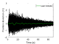
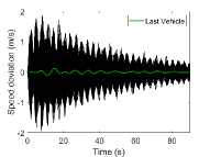
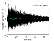
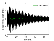
Simulations, illustrated in Figure 1, were performed by means of Matlab, using the second order Euler numerical method. In the simulations, we set v0=20m s1subscript𝑣020timesmetersecond1v_{0}=20~{}$\mathrm{m}\text{\,}{\mathrm{s}}^{-1}$ and δi,i1=δi+1,i=10msubscript𝛿𝑖𝑖1subscript𝛿𝑖1𝑖10meter\delta_{i,i-1}=\delta_{i+1,i}=10~{}$\mathrm{m}$ (note that any other inter-vehicle distance and reference speed profile could be selected as the optimization problem in Appendix C is independent on such parameters). In Figure 1, the time behavior is shown for the position and speed perturbations of a string of N=1000𝑁1000N=1000 vehicles when the perturbations di¯(t)=ηi5sin(t)exp(0.02t)¯subscript𝑑𝑖𝑡subscript𝜂𝑖5𝑡0.02𝑡\bar{d_{i}}(t)=\eta_{i}5\sin(t)\exp(-0.02t) are applied at time t=0𝑡0t=0 to 500500500 randomly selected vehicles (the parameters ηi[1,1]subscript𝜂𝑖11\eta_{i}\in[-1,1] are random scaling factors). This choice of di(t)subscript𝑑𝑖𝑡d_{i}(t)’s physically corresponds to realistic but strong disturbances (Monteil and Bouroche, 2016). Figure 1 clearly shows that, both the bidirectional and the predecessor-follower protocols designed so as to fulfill the conditions of Corollary 1 and Corollary 2, ensure a subscript\mathcal{L}_{\infty} string stable behavior. Also, in accordance to e.g. (Hao et al., 2012; Herman et al., 2017b; Nieuwenhuijze, 2010), we found in the simulations that the bidirectional control exhibits a better disturbance rejection for both the position and speed deviations (that is, the peak of the position deviation is observed to be at 2.2 mmeter\mathrm{m} for εi=0subscript𝜀𝑖0\varepsilon_{i}=0 and at 1.9 mmeter\mathrm{m} for εi=1subscript𝜀𝑖1\varepsilon_{i}=1, and the peak of the speed deviation is observed to be at 1.9 m s1timesmetersecond1\mathrm{m}\text{\,}{\mathrm{s}}^{-1} for εi=0subscript𝜀𝑖0\varepsilon_{i}=0 and at 1.7 m s1timesmetersecond1\mathrm{m}\text{\,}{\mathrm{s}}^{-1} for εi=1subscript𝜀𝑖1\varepsilon_{i}=1).

Refer to caption Refer to caption
Figure 1: Simulations for the platoon system of Section 4. Top panel: position/speed perturbations when $\varepsilon_{i}=0$, $\forall i$. Bottom panel: speed/position perturbations with $\varepsilon_{i}=1$, $\forall i$.

5 Conclusions

We presented a sufficient condition for the $\mathcal{L}_{\infty}$ string stability of asymmetrically coupled bidirectional heterogeneous, nonlinear, platoon systems. Our result directly links string stability to the design of the coupling protocols. We showed, via an example, how our result can be recast as an optimization problem and how this formulation can be used to design distributed control protocols for $\mathcal{L}_{\infty}$ string stable platoon systems. Future work will be aimed at studying: (i) whether automated vehicles can coexist with manually-driven vehicles and designing distributed control protocols supporting this mixed scenario; (ii) the possibility of devising a fully distributed control protocol for platoon systems by e.g. making use of feed-forward terms and/or nonlinear spacing policies.

Appendix

Appendix A Mathematical tools

Let $A$ be a complex $n\times n$ matrix. We recall that the matrix measure of the matrix $A$ induced by a $p$-vector norm, $\left|\cdot\right|_{p}$, is defined as $\mu_{p}(A):=\lim_{h\rightarrow 0^{+}}\frac{1}{h}\left(\left\|I+hA\right\|-1\right)$, see (Vidyasagar, 1993) and (Russo et al., 2010) where matrix measures are used in the context of nonlinear contraction analysis. In this paper we state our results in terms of $\mu_{2}(A):=\max_{i}\left(\lambda_{i}\left\{\frac{A+A^{T}}{2}\right\}\right)$, i.e. the matrix measure induced by the $2$-vector norm. Recall here that $p$-vector norms are monotone, i.e. $\forall x_{1},x_{2}\in{\mathbb{R}}^{n}$ such that $0\leq x_{1}\leq x_{2}$ it happens that $\left|x_{1}\right|_{p}\leq\left|x_{2}\right|_{p}$ (where $x_{1}\leq x_{2}$ is understood component-wise). We make use of the following result from (Russo et al., 2013).

Lemma 2.

Let: (i) $\left|\cdot\right|_{S}$ and $\mu_{S}(\cdot)$ be, respectively, any $p$-vector and its induced matrix measure on ${\mathbb{R}}^{N}$; (ii) $\left|\cdot\right|_{G}$ be the vector norm on ${\mathbb{R}}^{nN}$ defined as $\left|\xi\right|_{G}:=\left|[\left|\xi_{1}\right|_{L_{1}},\ldots,\left|\xi_{N}\right|_{L_{N}}]\right|_{S}$; (iii) $\mu_{G}(\cdot)$ be the matrix measure induced by $\left|\cdot\right|_{G}$. Finally, let $A:=(A_{ij})_{i,j=1}^{N}\in{\mathbb{R}}^{nN\times nN}$, with $A_{ij}\in{\mathbb{R}}^{n\times n}$ and let $\hat{A}:=(\hat{A}_{ij})_{i,j=1}^{N}\in{\mathbb{R}}^{N\times N}$, with $\hat{A}_{ii}:=\mu_{L_{i}}(A_{ii})$ and $\hat{A}_{ij}:=\left\|A_{ij}\right\|_{L_{i,j}}$, $\forall i,j=1,\ldots,N$. Then, $\mu_{G}(A)\leq\mu_{S}(\hat{A})$.

Appendix B Proofs of the technical results

Proof of Theorem 1

For the sake of convenience we rewrite (3) in a more compact form as $\dot{y}_{i}=g_{i}(t,Y)$, $i=1,\ldots,N$, with

$$\begin{split}g_{i}(t,Y)&:=f_{i}(y_{i})+\tilde{h}_{i,i-1}(t,y_{i-1},y_{i})\\ &+\varepsilon_{i}\tilde{h}_{i,i+1}(t,y_{i+1},y_{i})+\tilde{h}_{i,0}(t,y_{i},x_{0}).\end{split}$$ (14)

Also, we rewrite (1) - (2) as $\dot{x}_{i}=g_{i}(t,X)+d_{i}(t)$, $i=1,\ldots,N$, with the functions $g_{i}$’s defined as in (14).

Condition C1 implies that $Y^{\ast}(t)$ is a solution of the unperturbed dynamics (3). Let $z_{i}(t):=x_{i}(t)-y_{i}^{\ast}(t)$, $Z(t):=[z_{1}(t)^{T},\ldots,z_{N}(t)^{T}]^{T}$ and $d(t)$ being the stack of all $d_{i}$’s (if the disturbance does not affect the $i$-th vehicle, then $d_{i}(t)=0$). Now, following Theorem A in (Desoer and Haneda, 1972) (see also Theorem 3 in (Hamadeh et al., 2015) for a self-contained proof), the dynamics of $Z(t)$ can be expressed as

$$\dot{Z}(t)=A(t)Z(t)+d(t),$$ (15)

with $A(t):=\int_{0}^{1}\tilde{J}(t,\eta X+(1-\eta)Y)d\eta$ and where $\tilde{J}(t,X):=\frac{\partial G}{\partial X}$, with $G(t,X):=[g_{1}^{T}(t,X),\ldots,g_{N}^{T}(t,X)]^{T}$. Then, as shown in (Desoer and Haneda, 1972) and (Hamadeh et al., 2015), one gets

$$\begin{split}D^{+}\left|Z(t)\right|=&\mu(A(t))\left|Z(t)\right|+\left|d(t)\right|,\end{split}$$ (16)

where $D^{+}{\left|Z(t)\right|}$ is the Dini derivative of $\left|Z(t)\right|$, i.e. $D^{+}{\left|Z(t)\right|}:=\lim_{h\rightarrow 0^{+}}\sup\frac{1}{h}\left(\left|Z(t+h)\right|-\left|Z(t)\right|\right)$. Inequality (16) is valid for any vector norm and, in particular, it also holds when |Z|=|Z|G:=|[|z1|2,,|zN|2]|𝑍subscript𝑍𝐺assignsubscriptsubscriptsubscript𝑧12subscriptsubscript𝑧𝑁2\left|Z\right|=\left|Z\right|_{G}:=\left|\left[\left|z_{1}\right|_{{\color[rgb]{0,0,0}\definecolor[named]{pgfstrokecolor}{rgb}{0,0,0}\pgfsys@color@gray@stroke{0}\pgfsys@color@gray@fill{0}2}},\ldots,\left|z_{N}\right|_{{\color[rgb]{0,0,0}\definecolor[named]{pgfstrokecolor}{rgb}{0,0,0}\pgfsys@color@gray@stroke{0}\pgfsys@color@gray@fill{0}2}}\right]\right|_{{\color[rgb]{0,0,0}\definecolor[named]{pgfstrokecolor}{rgb}{0,0,0}\pgfsys@color@gray@stroke{0}\pgfsys@color@gray@fill{0}\infty}}. That is, by definition, $\left|Z\right|_{G}=\sup_{i}\left|z_{i}\right|_{2}$. Now, the rest of the proof is aimed at showing that there exists some $\bar{c}\neq 0$ such that $\mu_{G}\left(\tilde{J}(t,X)\right)\leq-\bar{c}^{2}$, $\forall t\geq t_{0}$ and $\forall X$ (indeed, by means of subadditivity of matrix measures this implies that $\mu(A(t))\leq-\bar{c}^{2}$). In order to show this, partition the matrix $\tilde{J}$ in $\tilde{J}=(\tilde{J}_{ij})_{i,j=1}^{N}$, with $\tilde{J}_{ij}\in{\mathbb{R}}^{n\times n}$. Then, by means of Lemma 2, we have that μG(J~)μ(J^)subscript𝜇𝐺~𝐽subscript𝜇^𝐽\mu_{G}(\tilde{J})\leq\mu_{{\color[rgb]{0,0,0}\definecolor[named]{pgfstrokecolor}{rgb}{0,0,0}\pgfsys@color@gray@stroke{0}\pgfsys@color@gray@fill{0}\infty}}(\hat{J}), where $\hat{J}:=(\hat{J}_{ij})_{i,j=1}^{N}\in{\mathbb{R}}^{N\times N}$:

J^ii=μ2(J~ii),i=1,,N,J^i,i+1=εiJ~i,i+12,i=1,,N1,J^i+1,i=J~i+1,i2,i=1,,N1.subscript^𝐽𝑖𝑖subscript𝜇2subscript~𝐽𝑖𝑖𝑖1𝑁missing-subexpressionmissing-subexpressionmissing-subexpressionmissing-subexpressionmissing-subexpressionmissing-subexpressionmissing-subexpressionmissing-subexpressionmissing-subexpressionmissing-subexpressionmissing-subexpressionmissing-subexpressionmissing-subexpressionmissing-subexpressionmissing-subexpressionmissing-subexpressionmissing-subexpressionmissing-subexpressionsubscript^𝐽𝑖𝑖1subscript𝜀𝑖subscriptnormsubscript~𝐽𝑖𝑖12𝑖1𝑁1missing-subexpressionmissing-subexpressionmissing-subexpressionmissing-subexpressionmissing-subexpressionmissing-subexpressionmissing-subexpressionmissing-subexpressionmissing-subexpressionmissing-subexpressionmissing-subexpressionmissing-subexpressionmissing-subexpressionmissing-subexpressionmissing-subexpressionmissing-subexpressionmissing-subexpressionmissing-subexpressionsubscript^𝐽𝑖1𝑖subscriptnormsubscript~𝐽𝑖1𝑖2𝑖1𝑁1missing-subexpressionmissing-subexpressionmissing-subexpressionmissing-subexpressionmissing-subexpressionmissing-subexpressionmissing-subexpressionmissing-subexpressionmissing-subexpressionmissing-subexpressionmissing-subexpressionmissing-subexpressionmissing-subexpressionmissing-subexpressionmissing-subexpressionmissing-subexpressionmissing-subexpressionmissing-subexpression\begin{array}[]{*{20}l}\hat{J}_{ii}=\mu_{{\color[rgb]{0,0,0}\definecolor[named]{pgfstrokecolor}{rgb}{0,0,0}\pgfsys@color@gray@stroke{0}\pgfsys@color@gray@fill{0}2}}\left(\tilde{J}_{ii}\right),&i=1,\ldots,N,\\ \hat{J}_{i,i+1}=\varepsilon_{i}\left\|\tilde{J}_{i,i+1}\right\|_{{\color[rgb]{0,0,0}\definecolor[named]{pgfstrokecolor}{rgb}{0,0,0}\pgfsys@color@gray@stroke{0}\pgfsys@color@gray@fill{0}2}},&i=1,\ldots,N-1,\\ \hat{J}_{i+1,i}=\left\|\tilde{J}_{i+1,i}\right\|_{{\color[rgb]{0,0,0}\definecolor[named]{pgfstrokecolor}{rgb}{0,0,0}\pgfsys@color@gray@stroke{0}\pgfsys@color@gray@fill{0}2}},&i=1,\ldots,N-1.\end{array} (17)

For convenience, in (17) and in what follows we are omitting the dependencies of the matrices $\tilde{J}_{ij}$’s on the state variables. Now, in order to show the result we need to show that there exists some $\bar{c}\neq 0$ such that μ(J^)c¯2subscript𝜇^𝐽superscript¯𝑐2\mu_{{\color[rgb]{0,0,0}\definecolor[named]{pgfstrokecolor}{rgb}{0,0,0}\pgfsys@color@gray@stroke{0}\pgfsys@color@gray@fill{0}\infty}}(\hat{J})\leq-\bar{c}^{2}, $\forall t\geq t_{0}$ and $\forall X$. Now, by definition on $\mu_{\infty}(\cdot)$, this is a row-dominance condition on the matrix $\hat{J}$. That is, we need to show that there exists some $\bar{c}\neq 0$ such that, $\forall X$:

$$\begin{array}[]{*{20}l}\mu_{2}\left(\tilde{J}_{ii}\right)+\varepsilon_{i}\left\|J_{i,i+1}\right\|_{2}+\left\|J_{i,i-1}\right\|_{2}\leq-\bar{c}^{2},&i=1,\ldots,N,\\ \end{array}$$ (18)

where we used the definition of the matrix $\hat{J}$ and, in order to make the notation more compact, we set J~i,j2=0subscriptnormsubscript~𝐽𝑖𝑗20\left\|\tilde{J}_{i,j}\right\|_{{\color[rgb]{0,0,0}\definecolor[named]{pgfstrokecolor}{rgb}{0,0,0}\pgfsys@color@gray@stroke{0}\pgfsys@color@gray@fill{0}2}}=0 whenever $i,j\notin\{1,\dots,N\}$. Now, by means of C2, the above expression can be upper bounded, for all $i=1,\ldots,N$, by: $-c^{2}+\left(1+\max_{i}\varepsilon_{i}\right)\bar{J}:=-\bar{c}^{2}$. In turn, from C3 we get $-c^{2}+\left(1+\max_{i}\varepsilon_{i}\right)\bar{J}<0$, thus implying that there exists some $\bar{c}\neq 0$ such that μ(J^)c¯2subscript𝜇^𝐽superscript¯𝑐2\mu_{{\color[rgb]{0,0,0}\definecolor[named]{pgfstrokecolor}{rgb}{0,0,0}\pgfsys@color@gray@stroke{0}\pgfsys@color@gray@fill{0}\infty}}(\hat{J})\leq-\bar{c}^{2}, $\forall X$. Together with (16), this implies that:

D+|Z(t)|Gc¯2|Z(t)|G+|d(t)|G.superscript𝐷subscript𝑍𝑡𝐺superscript¯𝑐2subscript𝑍𝑡𝐺subscript𝑑𝑡𝐺\begin{split}D^{+}{\left|Z(t)\right|}_{{\color[rgb]{0,0,0}\definecolor[named]{pgfstrokecolor}{rgb}{0,0,0}\pgfsys@color@gray@stroke{0}\pgfsys@color@gray@fill{0}G}}&\leq-\bar{c}^{2}\left|Z(t)\right|_{{\color[rgb]{0,0,0}\definecolor[named]{pgfstrokecolor}{rgb}{0,0,0}\pgfsys@color@gray@stroke{0}\pgfsys@color@gray@fill{0}G}}+\left|d(t)\right|_{{\color[rgb]{0,0,0}\definecolor[named]{pgfstrokecolor}{rgb}{0,0,0}\pgfsys@color@gray@stroke{0}\pgfsys@color@gray@fill{0}G}}.\end{split} (19)

From (19) we get D+|Z(t)|Gc¯2|Z(t)|G+supidi()superscript𝐷subscript𝑍𝑡𝐺superscript¯𝑐2subscript𝑍𝑡𝐺subscriptsupremum𝑖subscriptnormsubscript𝑑𝑖subscriptD^{+}{\left|Z(t)\right|}_{{\color[rgb]{0,0,0}\definecolor[named]{pgfstrokecolor}{rgb}{0,0,0}\pgfsys@color@gray@stroke{0}\pgfsys@color@gray@fill{0}G}}\leq-\bar{c}^{2}\left|Z(t)\right|_{{\color[rgb]{0,0,0}\definecolor[named]{pgfstrokecolor}{rgb}{0,0,0}\pgfsys@color@gray@stroke{0}\pgfsys@color@gray@fill{0}G}}+{\color[rgb]{0,0,0}\definecolor[named]{pgfstrokecolor}{rgb}{0,0,0}\pgfsys@color@gray@stroke{0}\pgfsys@color@gray@fill{0}\sup_{i}\left\|d_{i}(\cdot)\right\|_{\mathcal{L}_{\infty}}}, where we used the definition of $\left|\cdot\right|_{G}$ together with the definition of the supremum norm. Thus, application of the Gronwall’s inequality yields:

|Z(t)|Gec¯2(tt0)|Z(t0)|G+1ec¯2(tt0)c¯2supidi(),subscript𝑍𝑡𝐺superscript𝑒superscript¯𝑐2𝑡subscript𝑡0subscript𝑍subscript𝑡0𝐺1superscript𝑒superscript¯𝑐2𝑡subscript𝑡0superscript¯𝑐2subscriptsupremum𝑖subscriptnormsubscript𝑑𝑖subscript\left|Z(t)\right|_{{\color[rgb]{0,0,0}\definecolor[named]{pgfstrokecolor}{rgb}{0,0,0}\pgfsys@color@gray@stroke{0}\pgfsys@color@gray@fill{0}G}}\leq e^{-\bar{c}^{2}(t-t_{0})}\left|Z(t_{0})\right|_{{\color[rgb]{0,0,0}\definecolor[named]{pgfstrokecolor}{rgb}{0,0,0}\pgfsys@color@gray@stroke{0}\pgfsys@color@gray@fill{0}G}}+\frac{1-e^{-\bar{c}^{2}(t-t_{0})}}{\bar{c}^{2}}{\color[rgb]{0,0,0}\definecolor[named]{pgfstrokecolor}{rgb}{0,0,0}\pgfsys@color@gray@stroke{0}\pgfsys@color@gray@fill{0}\sup_{i}\left\|d_{i}(\cdot)\right\|_{\mathcal{L}_{\infty}}},

$\forall t\geq t_{0}$. Finally, since $Z(t):=X(t)-Y^{\ast}(t)$, this yields, by the definition of $\left|\cdot\right|_{G}$,

supi|xi(t)yi(t)|2ec¯2(tt0)supi|xi(t0)yi(t0)|2+1ec¯2(tt0)c¯2supidi(),subscriptsupremum𝑖subscriptsubscript𝑥𝑖𝑡superscriptsubscript𝑦𝑖𝑡2superscript𝑒superscript¯𝑐2𝑡subscript𝑡0subscriptsupremum𝑖subscriptsubscript𝑥𝑖subscript𝑡0superscriptsubscript𝑦𝑖subscript𝑡021superscript𝑒superscript¯𝑐2𝑡subscript𝑡0superscript¯𝑐2subscriptsupremum𝑖subscriptdelimited-∥∥subscript𝑑𝑖subscript\begin{split}\sup_{i}\left|x_{i}(t)-y_{i}^{\ast}(t)\right|_{{\color[rgb]{0,0,0}\definecolor[named]{pgfstrokecolor}{rgb}{0,0,0}\pgfsys@color@gray@stroke{0}\pgfsys@color@gray@fill{0}2}}&\leq e^{-\bar{c}^{2}(t-t_{0})}\sup_{i}\left|x_{i}(t_{0})-y_{i}^{\ast}(t_{0})\right|_{{\color[rgb]{0,0,0}\definecolor[named]{pgfstrokecolor}{rgb}{0,0,0}\pgfsys@color@gray@stroke{0}\pgfsys@color@gray@fill{0}2}}\\ &+\frac{1-e^{-\bar{c}^{2}(t-t_{0})}}{\bar{c}^{2}}{\color[rgb]{0,0,0}\definecolor[named]{pgfstrokecolor}{rgb}{0,0,0}\pgfsys@color@gray@stroke{0}\pgfsys@color@gray@fill{0}\sup_{i}\left\|d_{i}(\cdot)\right\|_{\mathcal{L}_{\infty}}},\end{split}

$\forall t\geq t_{0}$ and this gives the result.∎

Proof of Corollary 1

Apply, to the dynamics (5) - (6), the coordinate transformation $\tilde{x}_{i}:=T_{i}x_{i}$, where $T_{i}$ is given as in (7). This yields the transformed dynamics:

x~˙i=TiFTi1x~i+TiB(hi,i1(Ti11x~i1,Ti1x~i)++εihi,i+1(Ti+11x~i+1,Ti1x~i)+hi(0)(Ti1x~i,x0))+d~i(t),subscript˙~𝑥𝑖subscript𝑇𝑖𝐹superscriptsubscript𝑇𝑖1subscript~𝑥𝑖subscript𝑇𝑖𝐵subscript𝑖𝑖1superscriptsubscript𝑇𝑖11subscript~𝑥𝑖1superscriptsubscript𝑇𝑖1subscript~𝑥𝑖subscript𝜀𝑖subscript𝑖𝑖1superscriptsubscript𝑇𝑖11subscript~𝑥𝑖1superscriptsubscript𝑇𝑖1subscript~𝑥𝑖superscriptsubscript𝑖0superscriptsubscript𝑇𝑖1subscript~𝑥𝑖subscript𝑥0subscript~𝑑𝑖𝑡\begin{split}&\dot{\tilde{x}}_{i}=T_{i}FT_{i}^{-1}\tilde{x}_{i}+T_{i}B\left(h_{i,i-1}(T_{i-1}^{-1}\tilde{x}_{i-1},T_{i}^{-1}\tilde{x}_{i})+\right.\\ &\left.+\varepsilon_{i}h_{i,i+1}(T_{i+1}^{-1}\tilde{x}_{i+1},T_{i}^{-1}\tilde{x}_{i})+{\color[rgb]{0,0,0}\definecolor[named]{pgfstrokecolor}{rgb}{0,0,0}\pgfsys@color@gray@stroke{0}\pgfsys@color@gray@fill{0}h_{i}^{(0)}}(T_{i}^{-1}\tilde{x}_{i},x_{0})\right)+\tilde{d}_{i}(t),\end{split} (20)

with $B:=[0,1]^{T}$ and $\tilde{d}_{i}(t)=T_{i}d_{i}(t)$. Let $\tilde{y}_{d,i}:=T_{i}y_{d,i}$, then the unperturbed dynamics of (20) is

y~˙i=TiFTi1y~i+TiB(hi,i1(Ti11y~i1,Ti1y~i)++εihi,i+1(Ti+11y~i+1,Ti1y~i)+hi(0)(Ti1y~i,x0)).subscript˙~𝑦𝑖subscript𝑇𝑖𝐹superscriptsubscript𝑇𝑖1subscript~𝑦𝑖subscript𝑇𝑖𝐵subscript𝑖𝑖1superscriptsubscript𝑇𝑖11subscript~𝑦𝑖1superscriptsubscript𝑇𝑖1subscript~𝑦𝑖subscript𝜀𝑖subscript𝑖𝑖1superscriptsubscript𝑇𝑖11subscript~𝑦𝑖1superscriptsubscript𝑇𝑖1subscript~𝑦𝑖superscriptsubscript𝑖0superscriptsubscript𝑇𝑖1subscript~𝑦𝑖subscript𝑥0\begin{split}&\dot{\tilde{y}}_{i}=T_{i}FT_{i}^{-1}\tilde{y}_{i}+T_{i}B\left(h_{i,i-1}(T_{i-1}^{-1}\tilde{y}_{i-1},T_{i}^{-1}\tilde{y}_{i})+\right.\\ &\left.+\varepsilon_{i}h_{i,i+1}(T_{i+1}^{-1}\tilde{y}_{i+1},T_{i}^{-1}\tilde{y}_{i})+{\color[rgb]{0,0,0}\definecolor[named]{pgfstrokecolor}{rgb}{0,0,0}\pgfsys@color@gray@stroke{0}\pgfsys@color@gray@fill{0}h_{i}^{(0)}}(T_{i}^{-1}\tilde{y}_{i},x_{0})\right).\end{split} (21)

Now, it suffices to note that: (i) the fulfillment of C1 of Corollary 1 implies the fulfillment of C1 of Theorem 1; (ii) differentiation of (20) yields the Jacobian matrix $J:=(J_{ij})_{i,j=1}^{N}\in{\mathbb{R}}^{2N\times 2N}$, where each element $J_{ij}\in{\mathbb{R}}^{2\times 2}$ is given by (8). In turn, this means that the fulfillment of conditions C2 - C3 of Corollary 1 implies that the same conditions of Theorem 1 are also fulfilled for the dynamics (20).

Thus, application of Theorem 1 to the dynamics (20) with $y_{i}^{\ast}(t)=\tilde{y}_{d,i}(t)$ yields supi|x~i(t)y~d,i(t)|2ec¯2tsupi|x~i(0)y~d,i(0)|2+1ec¯2tc¯2supid~i()subscriptsupremum𝑖subscriptsubscript~𝑥𝑖𝑡subscript~𝑦𝑑𝑖𝑡2superscript𝑒superscript¯𝑐2𝑡subscriptsupremum𝑖subscriptsubscript~𝑥𝑖0subscript~𝑦𝑑𝑖021superscript𝑒superscript¯𝑐2𝑡superscript¯𝑐2subscriptsupremum𝑖subscriptnormsubscript~𝑑𝑖subscript\sup_{i}\left|\tilde{x}_{i}(t)-\tilde{y}_{d,i}(t)\right|_{{\color[rgb]{0,0,0}\definecolor[named]{pgfstrokecolor}{rgb}{0,0,0}\pgfsys@color@gray@stroke{0}\pgfsys@color@gray@fill{0}2}}\leq e^{-\bar{c}^{2}t}\sup_{i}\left|\tilde{x}_{i}(0)-\tilde{y}_{d,i}(0)\right|_{{\color[rgb]{0,0,0}\definecolor[named]{pgfstrokecolor}{rgb}{0,0,0}\pgfsys@color@gray@stroke{0}\pgfsys@color@gray@fill{0}2}}+\frac{1-e^{-\bar{c}^{2}t}}{\bar{c}^{2}}\sup_{i}\left\|\tilde{d}_{i}(\cdot)\right\|_{\mathcal{L}_{\infty}}, $\forall t\geq 0$. Now:

supi|x~i(t)y~d,i(t)|2λ¯supi|xi(t)yd,i(t)|2,subscriptsupremum𝑖subscriptsubscript~𝑥𝑖𝑡subscript~𝑦𝑑𝑖𝑡2¯𝜆subscriptsupremum𝑖subscriptsubscript𝑥𝑖𝑡subscript𝑦𝑑𝑖𝑡2\begin{split}\sup_{i}\left|\tilde{x}_{i}(t)-\tilde{y}_{d,i}(t)\right|_{{\color[rgb]{0,0,0}\definecolor[named]{pgfstrokecolor}{rgb}{0,0,0}\pgfsys@color@gray@stroke{0}\pgfsys@color@gray@fill{0}2}}\geq\underline{\lambda}\sup_{i}\left|x_{i}(t)-y_{d,i}(t)\right|_{{\color[rgb]{0,0,0}\definecolor[named]{pgfstrokecolor}{rgb}{0,0,0}\pgfsys@color@gray@stroke{0}\pgfsys@color@gray@fill{0}2}},\end{split} (22)

where $\underline{\lambda}:=\min_{i}\left\{\sigma_{\min}(T_{i})\right\}$. Also:

supi|x~i(0)y~d,i(0)|2λ¯supi|xi(0)yd,i(0)|2,subscriptsupremum𝑖subscriptsubscript~𝑥𝑖0subscript~𝑦𝑑𝑖02¯𝜆subscriptsupremum𝑖subscriptsubscript𝑥𝑖0subscript𝑦𝑑𝑖02\begin{split}\sup_{i}\left|\tilde{x}_{i}(0)-\tilde{y}_{d,i}(0)\right|_{{\color[rgb]{0,0,0}\definecolor[named]{pgfstrokecolor}{rgb}{0,0,0}\pgfsys@color@gray@stroke{0}\pgfsys@color@gray@fill{0}2}}&\leq\bar{\lambda}\sup_{i}\left|x_{i}(0)-y_{d,i}(0)\right|_{{\color[rgb]{0,0,0}\definecolor[named]{pgfstrokecolor}{rgb}{0,0,0}\pgfsys@color@gray@stroke{0}\pgfsys@color@gray@fill{0}2}},\end{split} (23)

where $\bar{\lambda}:=\max_{i}\left\{\sigma_{\max}(T_{i})\right\}$. Finally, we have:

$$\begin{split}\sup_{i}\left\|\tilde{d}_{i}(\cdot)\right\|_{\mathcal{L}_{\infty}}\leq\max_{i}\left\{\sigma_{\max}(T_{i})\right\}\sup_{i}\left\|d_{i}(\cdot)\right\|_{\mathcal{L}_{\infty}}.\end{split}$$ (24)

Then, (10) directly follows from (22) - (24). ∎

Appendix C Recasting C2 and C3 as an optimization problem

Formally, finding the set of control gains $K_{vi}$, $K_{vi,0}$, $K_{pi,0}$, $K_{pi,1}$, $K_{pi,2}$, fulfilling C2 and C3 can be recast as the following optimization problem:

minKvi,Kpi,0,Kpi,1,Kpi,2,Kvi,0,αi,C,J¯,εi𝒥(Kvi,Kvi,0,Kpi,0,Kpi,1,Kpi,2,εi)s.t.Kvi>0,Kpi,0>0,Kvi,0>0,Kpi,1>0,Kpi,2>0,J¯>0,C>0,αi>0,0εi1μ2(Ji,i(αi,xi,xi1,εi))C,(εi+1)J¯<C,Ji,i1(αi,xi,xi1)2J¯,Ji,i+1(αi,xi,xi+1)2J¯,\begin{split}&\min_{\begin{array}[]{*{20}c}K_{vi},K_{pi,0},K_{pi,1},\\ K_{pi,2},K_{vi,0},\alpha_{i},C,\bar{J},\varepsilon_{i}\end{array}}\mathcal{J}\left(K_{vi},K_{vi,0},K_{pi,0},K_{pi,1},K_{pi,2},\varepsilon_{i}\right)\\ &\text{s.t.}\\ &K_{vi}>0,\quad K_{pi,0}>0,\quad K_{vi,0}>0,\quad K_{pi,1}>0,\\ &K_{pi,2}>0,\quad\bar{J}>0,\quad C>0,\quad\alpha_{i}>0,\quad 0\leq\varepsilon_{i}\leq 1\\ &\mu_{2}\left(J_{i,i}(\alpha_{i},x_{i},x_{i-1},\varepsilon_{i})\right)\leq-C,\quad\left(\varepsilon_{i}+1\right)\bar{J}<C,\\ &\left\|J_{i,i-1}(\alpha_{i},x_{i},x_{i-1})\right\|_{{\color[rgb]{0,0,0}\definecolor[named]{pgfstrokecolor}{rgb}{0,0,0}\pgfsys@color@gray@stroke{0}\pgfsys@color@gray@fill{0}2}}\leq\bar{J},\quad\left\|J_{i,i+1}(\alpha_{i},x_{i},x_{i+1})\right\|_{{\color[rgb]{0,0,0}\definecolor[named]{pgfstrokecolor}{rgb}{0,0,0}\pgfsys@color@gray@stroke{0}\pgfsys@color@gray@fill{0}2}}\leq\bar{J},\\ \end{split} (25)

where the decision variables are the control gains and the auxiliary variables $\alpha_{i}$, $C$, $\bar{J}$. We set $\mathcal{J}\left(\cdot\right)=-\bar{g_{i}}=-K_{pi,1}K_{pi,2}$ and solve the above problem for fixed $\alpha_{i}>0$ and $0\leq\varepsilon_{i}\leq 1$. With this choice of the cost function, the upper bound of $\partial g_{i}/\partial x$ is maximized (note that other cost functions can be considered as the steps described below are not dependent on $\mathcal{J}(\cdot)$). Now, we recast the constraints in (25) as LMIs, see e.g. (Boyd et al., 1994): (i) by definition, the constraint $\mu_{2}\left(J_{i,i}\right)\leq-C$ is equivalent to $[J_{i,i}]_{s}\prec-CI_{2}$; (ii) by definition, the constraint Ji,i1(αi,xi,xi1)2J¯subscriptnormsubscript𝐽𝑖𝑖1subscript𝛼𝑖subscript𝑥𝑖subscript𝑥𝑖12¯𝐽\left\|J_{i,i-1}(\alpha_{i},x_{i},x_{i-1})\right\|_{{\color[rgb]{0,0,0}\definecolor[named]{pgfstrokecolor}{rgb}{0,0,0}\pgfsys@color@gray@stroke{0}\pgfsys@color@gray@fill{0}2}}\leq\bar{J} is equivalent to $\bar{J}^{2}I_{2}-J_{i,i-1}J_{i,i-1}^{T}\succeq 0$ and hence, by means of the Schur complement, see e.g. (Horn and Johnson, 2013, Theorem $7.7.7$) and dividing by $\bar{J}>0$, this is in turn equivalent to $\begin{bmatrix}\bar{J}\cdot I_{2}&J_{i,i-1}\\ J_{i,i-1}^{T}&\bar{J}\cdot I_{2}\end{bmatrix}\succeq 0$. Moreover, as $J_{i,i-1}$ and $J_{i,i}$ both depend linearly on $\partial g_{i}/\partial x$ and $0\leq\partial g_{i}/\partial x\leq\bar{g_{i}}$, then the above constraints define convex sets. Therefore: (i) $[J_{i,i}]_{s}\prec-CI_{2}$ can be replaced by the pair of constraints $[J_{i,i,lb}]_{s}\prec-CI_{2}$ and $[J_{i,i,ub}]_{s}\prec-CI_{2}$; (ii) $\left\|J_{i,i-1}\right\|_{2}\leq\bar{J}$ can be replaced by the pair of constraints $\left\|J_{i,i-1,lb}\right\|_{2}\leq\bar{J}$ and $\left\|J_{i,i-1,ub}\right\|_{2}\leq\bar{J}$ (see (27) below for the definition of the matrices). This yields to the convex optimization problem solved in Section 4:

$$\begin{split}&\min_{K_{vi},K_{pi,0},K_{vi,0},\bar{g_{i}},C,\bar{J}}-\bar{g_{i}},\quad\text{subject to:}\\ &\quad K_{vi}>0,\quad K_{pi,0}>0,\quad K_{vi,0}>0,\quad\bar{g_{i}}>0,\quad\bar{J}>0,\\ &\quad C>0,\quad\alpha_{i}>0,\quad 0\leq\varepsilon_{i}\leq 1,\quad\left(\varepsilon_{i}+1\right)\bar{J}-C<0,\\ &\begin{bmatrix}\bar{J}\cdot I_{2}&J_{i,i-1,lb}\\ J_{i,i-1,lb}^{T}&\bar{J}\cdot I_{2}\end{bmatrix}\succeq 0,\quad\begin{bmatrix}\bar{J}\cdot I_{2}&J_{i,i-1,ub}\\ J_{i,i-1,ub}^{T}&\bar{J}\cdot I_{2}\end{bmatrix}\succeq 0,\\ &\quad[J_{i,i,lb}]_{s}\prec-CI_{2},\quad[J_{i,i,ub}]_{s}\prec-CI_{2}.\end{split}$$ (26)

In our implementation in Section 4, the above problem was solved numerically for different values of $\alpha_{i}$ and $\varepsilon_{i}$. For any choice of such parameters, the solver was always able to converge to an optimal solution, thus returning a set of control gains minimizing the cost function. In the simulations of Section 4 we made use of the set of control gain that was returning the lowest value of the cost function across all the numerical experiments. The files implementing the optimization problem can be made available upon request.

$$\begin{split}&[J_{i,i,lb}]_{s}:=\begin{bmatrix}-\alpha_{i}K_{pi,0}&1+\alpha_{i}^{2}K_{pi,0}-\alpha_{i}\left(\left(1+\varepsilon_{i}\right)K_{vi}+K_{vi,0}\right)\\ -K_{pi,0}&\alpha_{i}K_{pi,0}-(1+\varepsilon_{i})K_{vi}-K_{vi,0}\end{bmatrix},\quad\quad\quad\quad\quad\quad\quad\quad J_{i,i-1,lb}:=\begin{bmatrix}0&\alpha_{i}K_{vi}\\ 0&K_{vi}\end{bmatrix}\\ &[J_{i,i,ub}]_{s}:=\begin{bmatrix}-\alpha_{i}K_{pi,0}&1+\alpha_{i}^{2}\left((1+\varepsilon_{i})\bar{g_{i}}+K_{pi,0}\right)-\alpha_{i}\left(\left(1+\varepsilon_{i}\right)K_{vi}+K_{vi,0}\right)\\ -K_{pi,0}&\alpha_{i}\left((1+\varepsilon_{i})\bar{g_{i}}+K_{pi,0}\right)-(1+\varepsilon_{i})K_{vi}-K_{vi,0}\end{bmatrix},\quad J_{i,i-1,ub}:=\begin{bmatrix}\alpha_{i}\bar{g}_{i}&-\alpha_{i}^{2}\bar{g}_{i}+\alpha_{i}K_{vi}\\ \bar{g}_{i}&-\alpha_{i}\bar{g}_{i}+K_{vi}\end{bmatrix}.\\ \end{split}$$ (27)

References

  • Alam et al. (2015) Alam, A., Besselink, B., Turri, V., Martensson, J., Johansson, K. H., 2015. Heavy-duty vehicle platooning for sustainable freight transportation: A cooperative method to enhance safety and efficiency. IEEE Control Systems 35 (6), 34–56.
  • Bando et al. (1995) Bando, M., Hasebe, K., Nakayama, A., Shibata, A., Sugiyama, Y., 1995. Dynamical model of traffic congestion and numerical simulation. Physical review E 51 (2), 1035.
  • Barooah et al. (2009) Barooah, P., Mehta, P. G., Hespanha, J. P., 2009. Mistuning-based control design to improve closed-loop stability margin of vehicular platoons. IEEE Transactions on Automatic Control 54 (9), 2100–2113.
  • Besselink and Johansson (2017) Besselink, B., Johansson, K. H., 2017. String stability and a delay-based spacing policy for vehicle platoons subject to disturbances. IEEE Transactions on Automatic Control 62 (9), 4376–4391.
  • Boyd et al. (1994) Boyd, S., El Ghaoui, L., Feron, E., Balakrishnan, V., 1994. Linear Matrix Inequalities in System and Control Theory. Society for Industrial and Applied Mathematics.
  • de Wit and Brogliato (1999) de Wit, C. C., Brogliato, B., 1999. Stability issues for vehicle platooning in automated highway systems. In: Proceedings of the 1999 IEEE International Conference on Control Applications. Vol. 2. pp. 1377–1382.
  • Desoer and Haneda (1972) Desoer, C., Haneda, H., 1972. The measure of a matrix as a tool to analyze computer algorithms for circuit analysis. IEEE Transactions on Circuit Theory 19 (5), 480–486.
  • di Bernardo et al. (2015) di Bernardo, M., Salvi, A., Santini, S., 2015. Distributed consensus strategy for platooning of vehicles in the presence of time-varying heterogeneous communication delays. IEEE Transactions on Intelligent Transportation Systems 16 (1), 102–112.
  • Hamadeh et al. (2015) Hamadeh, A., Sontag, E., Vecchio, D. D., Dec 2015. A contraction approach to input tracking via high gain feedback. In: 2015 54th IEEE Conference on Decision and Control (CDC). pp. 7689–7694.
  • Hao et al. (2011) Hao, H., Barooah, P., Mehta, P. G., 2011. Stability margin scaling laws for distributed formation control as a function of network structure. IEEE Transactions on Automatic Control 56 (4), 923–929.
  • Hao et al. (2012) Hao, H., Yin, H., Kan, Z., 2012. On the robustness of large 1-D network of double integrator agents. In: American Control Conference (ACC), 2012. IEEE, pp. 6059–6064.
  • Herman et al. (2017a) Herman, I., Knorn, S., Ahlén, A., 2017a. Disturbance scaling in bidirectional vehicle platoons with different asymmetry in position and velocity coupling. Automatica 82 (Supplement C), 13 – 20.
  • Herman et al. (2017b) Herman, I., Martinec, D., Hurák, Z., Sebek, M., 2017b. Scaling in bidirectional platoons with dynamic controllers and proportional asymmetry. IEEE Transactions on Automatic Control 62 (4), 2034–2040.
  • Horn and Johnson (2013) Horn, R. A., Johnson, C. R., 2013. Matrix Analysis, 2nd Edition. Cambridge University Press (Cambridge, UK).
  • Khalil (2002) Khalil, H. K., 2002. Nonlinear Systems, 3rd Edition. Prentice Hall.
  • Knorn et al. (2014) Knorn, S., Donaire, A., Agüero, J. C., Middleton, R. H., 2014. Passivity-based control for multi-vehicle systems subject to string constraints. Automatica 50 (12), 3224–3230.
  • Knorn et al. (2015) Knorn, S., Donaire, A., Agüero, J. C., Middleton, R. H., 2015. Scalability of bidirectional vehicle strings with static and dynamic measurement errors. Automatica 62, 208–212.
  • Levine and Athans (1966) Levine, W. S., Athans, M., 1966. On the optimal error regulation of a string of moving vehicles. IEEE Transactions on Automatic Control 11 (3), 355–361.
  • Martinec et al. (2016) Martinec, D., Herman, I., Sebek, M., 2016. On the necessity of symmetric positional coupling for string stability. IEEE Transactions on Control of Network Systems in press.
  • Middleton and Braslavsky (2010) Middleton, R. H., Braslavsky, J. H., 2010. String instability in classes of linear time invariant formation control with limited communication range. IEEE Transactions on Automatic Control 55 (7), 1519–1530.
  • Monteil and Bouroche (2016) Monteil, J., Bouroche, M., 2016. Robust parameter estimation of car-following models considering practical non-identifiability. In: Intelligent Transportation Systems (ITSC), 2016 IEEE 19th International Conference on. IEEE, pp. 581–588.
  • Monteil et al. (2018) Monteil, J., Bouroche, M., Leith, D. J., 2018. $\mathcal{L}_{2}$ and $\mathcal{L}_{\infty}$ stability analysis of heterogeneous traffic with application to parameter optimization for the control of automated vehicles. IEEE Transactions on Control Systems Technology, 1–16.
  • Monteil and Russo (2017) Monteil, J., Russo, G., 2017. On the design of nonlinear distributed control protocols for platooning systems. IEEE Control Systems Letters 1 (1), 140–145.
  • Nieuwenhuijze (2010) Nieuwenhuijze, M., 2010. String stability analysis of bidirectional adaptive cruise control. Tech. rep.
    URL https://pdfs.semanticscholar.org/8c15/21120989e3925e0f27d4cf720ba71296c685.pdf
  • Peppard (1974) Peppard, L., 1974. String stability of relative-motion PID vehicle control systems. IEEE Transactions on Automatic Control 19 (5), 579–581.
  • Ploeg et al. (2014a) Ploeg, J., Shukla, D. P., van de Wouw, N., Nijmeijer, H., 2014a. Controller synthesis for string stability of vehicle platoons. IEEE Transactions on Intelligent Transportation Systems 15 (2), 854–865.
  • Ploeg et al. (2014b) Ploeg, J., Van de Wouw, N., Nijmeijer, H., 2014b. $\mathcal{L}_{p}$ string stability of cascaded systems: Application to vehicle platooning. Control Systems Technology, IEEE Transactions on 22 (2), 786–793.
  • Rogge and Aeyels (2008) Rogge, J. A., Aeyels, D., 2008. Vehicle platoons through ring coupling. IEEE Transactions on Automatic Control 53 (6), 1370–1377.
  • Russo et al. (2010) Russo, G., Di Bernardo, M., Sontag, E. D., 2010. Global entrainment of transcriptional systems to periodic inputs. PLoS Comput Biol 6 (4), e1000739.
  • Russo et al. (2013) Russo, G., di Bernardo, M., Sontag, E. D., 2013. A contraction approach to the hierarchical analysis and design of networked systems. IEEE Transactions on Automatic Control 58, 1328–1331.
  • Seiler et al. (2004) Seiler, P., Pant, A., Hedrick, K., 2004. Disturbance propagation in vehicle strings. IEEE Transactions on Automatic Control 49 (10), 1835–1842.
  • Sheikholeslam and Desoer (1990) Sheikholeslam, S., Desoer, C. A., 1990. Longitudinal control of a platoon of vehicles. III, nonlinear model. California Partners for Advanced Transit and Highways (PATH).
  • Sontag (2008) Sontag, E. D., 2008. Input to state stability: Basic concepts and results. In: Nonlinear and optimal control theory. Springer, pp. 163–220.
  • Stuedli et al. (2017) Stuedli, S., Seron, M. M., Middleton, R. H., 2017. Vehicular platoons in cyclic interconnections with constant inter-vehicle spacing. IFAC-PapersOnLine 50 (1), 2511 – 2516, 20th IFAC World Congress.
  • Swaroop and Hedrick (1999) Swaroop, D., Hedrick, J., 1999. Constant spacing strategies for platooning in automated highway systems. Journal of Dynamic Systems, Measurement, and Control 121, 426 – 470.
  • Swaroop and Hedrick (1996) Swaroop, D., Hedrick, J. K., 1996. String stability of interconnected systems. IEEE Transactions on Automatic Control 41 (3), 349–357.
  • Swaroop et al. (2017) Swaroop, D., Konduri, S., Pagilla, P. R., May 2017. Effects of V2V communication on time headway for autonomous vehicles. In: 2017 American Control Conference (ACC). pp. 2002–2007.
  • Swaroop and Rajagopal (2001) Swaroop, D., Rajagopal, K. R., 2001. A review of constant time headway policy for automatic vehicle following. In: ITSC 2001. 2001 IEEE Intelligent Transportation Systems. Proceedings (Cat. No.01TH8585). pp. 65–69.
  • Vidyasagar (1993) Vidyasagar, M., 1993. Nonlinear systems analysis (2nd Ed.). Pretice-Hall (Englewood Cliffs, NJ, USA).
  • Yanakiev and Kanellakopoulos (1998) Yanakiev, D., Kanellakopoulos, I., 1998. Nonlinear spacing policies for automated heavy-duty vehicles. IEEE Transactions on Vehicular Technology 47 (4), 1365–1377.
  • Zegers et al. (2017) Zegers, J. C., Semsar-Kazerooni, E., Ploeg, J., van de Wouw, N., Nijmeijer, H., 2017. Consensus control for vehicular platooning with velocity constraints. IEEE Transactions on Control Systems Technology in press, 1–14.
  • Zheng et al. (2016) Zheng, Y., Li, S. E., Li, K., Wang, L. Y., 2016. Stability margin improvement of vehicular platoon considering undirected topology and asymmetric control. IEEE Transactions on Control Systems Technology 24 (4), 1253–1265.