Automatic Detection and Positioning of Ground Control Points Using TerraSAR-X Multi-Aspect Acquisitions

Abstract

This is the pre-acceptance version, to read the final version please go to IEEE Transactions on Geoscience and Remote Sensing on IEEE XPlore. (DOI: 10.1109/TGRS.2017.2769078)
Geodetic stereo Synthetic Aperture Radar (SAR) is capable of absolute three-dimensional localization of natural Persistent Scatterer (PS)s which allows for Ground Control Point (GCP) generation using only SAR data. The prerequisite for the method to achieve high precision results is the correct detection of common scatterers in SAR images acquired from different viewing geometries. In this contribution, we describe three strategies for automatic detection of identical targets in SAR images of urban areas taken from different orbit tracks. Moreover, a complete work-flow for automatic generation of large number of GCPs using SAR data is presented and its applicability is shown by exploiting TerraSAR-X (TS-X) high resolution spotlight images over the city of Oulu, Finland and a test site in Berlin, Germany.

I Introduction

sar imaging geodesy and geodetic stereo sar are relatively new techniques which aim at high precision absolute positioning of point targets in sar images in 2D and 3D, respectively [1, 2, 3]. The accuracy of both methods, when coupled with data from tsx and TanDEM-X, is in the centimeter regime for targets with accurately known phase centers such as corner reflectors [3]. This level of accuracy is achievable due to the precise orbit determination [4] and instrument calibration of the aforementioned satellites followed by a thorough correction scheme which quantifies and removes the most prominent error sources affecting radar timing measurements. This paves the way for remotely sensed generation of gcps using only sar data.

The essential prerequisite for applying the geodetic stereo sar method is the correct detection of identical scatterers in sar images acquired from different geometries. In this regard, a target can be visible only from same-heading orbits, i.e. exclusively ascending or descending orbits, or also from cross-heading orbits, which include combinations of ascending and descending orbits. Conceptually, a target localized from the latter is favorable because of the more robust intersection geometry when compared to the former. This fact is demonstrated in Fig. 1(a) where the intersection angle occurs at almost $90^{\circ}$ because of the large baseline between the satellites from cross-heading tracks. In Fig. 1(b), the target is localized with satellites from same-heading tracks which force the baseline to be smaller and consequently the system of equations to solve for the 3D coordinates to be less sensitive for the perpendicular height direction. However, the rare occurrence of identical scatterers visible from cross-heading configurations as well as the challenging task of automatically detecting such targets, either from same- or cross-heading tracks, currently limit the applicability of geodetic stereo sar for localization of large number of pss.

To overcome the limitation to some extent, this paper describes an automatic algorithm for detection and absolute positioning of large number of natural pss in sar images of urban areas. The candidates are selected from both same-heading and cross-heading geometries based on methods relying on fusion of multitrack psi point clouds, correspondence detection with optical data and utilizing vectorized road network data. The candidates are mainly chosen from the same-heading configuration because of the fact that for many pss the phase centers are assumed to remain unchanged in sar images. On the other hand, additional candidates are chosen from cross-heading geometries, although in a small number, because conceptually they can be localized more precisely compared to the candidates from same-heading geometries. Coupled with the subsequent geodetic Stereo sar, the proposed processing chain delivers sets of absolutely localized pss in an investigated area.

The remainder of the paper is organized as follows. Section II reviews the theoretical background of the techniques utilized in this study and gives an overview of the recent advances and the motivation for this work. Section III describes three methods for detecting identical pss visible in sar images from same- and cross-heading tracks. In Section IV, the complete work-flow for generating high precision absolute gcps is explained. In section V, the applicability of the algorithm is demonstrated by exploiting tsx high resolution spotlight images over the city of Oulu, Finland and a test site in Berlin, Germany, and finally the conclusions are drawn in section VI.

II High Precision Absolute 2D and 3D Positioning with tsx

At the core of high precision absolute positioning of candidate gcps using sar data are the imaging geodesy and the stereo sar methods. These methods are described in this section followed by the recent advances and applications which rely on absolute localization capability of tsx. It is important to note that the complete explanation of the theory of the methods and their practical implementations are not in the scope of this paper. For full treatment of these topics, the interested reader is referred to [1, 2, 3, 4, 5, 6, 7].

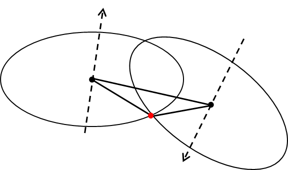
(a) Cross-heading

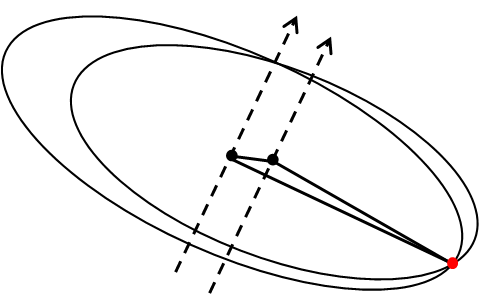
(b) Same-heading

Figure 1: Localization of a point target (red dot) from (a) cross-heading and (b) same-heading satellite tracks. The satellites are shown by black dots; their trajectories are presented by dashed lines and the baselines are depicted by solid lines between the satellite positions. The black circles are defined by the range-Doppler equations and their intersection leads to the 3D position of the target.

II-A Background

The sar imaging geodesy technique aims at achieving 2D absolute pixel localization [1]. Based on the sar measurement principle, a single pixel in a focused complex sar image, processed to zero-Doppler coordinates, is characterized with two time tags: in the along-track direction, the time relative to the time of the closest approach defines the azimuth coordinate $t_{az}$ and in the across-track direction, the difference in the time travel of the transmitted and the received chirp at $t_{az}$ describes the range coordinate $\tau_{rg}$ [8]. If we measure the radar timing coordinates ($t_{az}$, $\tau_{rg}$) for a point target located within the mentioned pixel, the following equations hold:

$$\tau_{rg}=\frac{2R}{c}+\delta\tau_{SD}+\delta\tau_{O}+\delta\tau_{F}+\delta\tau_{I}+\delta\tau_{T}+\delta\tau_{G},$$ (1)

$$t_{az}=t+\delta t_{SD}+\delta t_{O}+\delta t_{F}+\delta t_{G},$$ (2)

where $R$ is the geometric distance from the satellite to the center of the pixel in meters and $c$ is the speed of light in vacuum in $m/s$ while all the other terms are expressed in seconds; $t$ is the raw acquisition time, $\delta\tau_{SD}$ and $\delta t_{SD}$ are delays caused by satellite dynamics and electronics, $\delta\tau_{O}$ and $\delta t_{O}$ are the orbit inaccuracies, $\delta\tau_{F}$ and $\delta t_{F}$ are the feature localization error, $\delta\tau_{G}$ and $\delta t_{G}$ include the geodynamic effects all on range and azimuth timings, respectively while $\delta\tau_{I}$ and $\delta\tau_{T}$ are the ionospheric and the tropospheric delays considered only for range timings. The magnitude of the individual effects can be scaled to units of length by multiplying the range error terms with $\frac{c}{2}$ and the azimuth error terms with the platform’s velocity. The outcomes vary from a couple of centimeters for the ionospheric effect, if the satellite operates in X-band, followed by decimeter regimes for satellite electronic delays and geodynamic effects for both components, to up to four meters for the tropospheric effect depending on the average incidence angle of the acquired TS-X images.

Imaging geodesy corrects for all the error terms in (1) and (2) thus obtaining absolute range and azimuth timings. In this regard, the technique reduces the satellite dynamics effects by avoiding the stop-go approximation in the tmsp and by taking into account the non-zero duration of the pulses and the internal delay caused by the instrument cables [9]. The propagation errors are estimated based on the path delays derived from the near-by gnss stations or 3D integration through weather models followed by appropriate mapping functions [2, 3, 10]. For the geodynamic effects such as solid earth tides, plate tectonics, ocean loading and atmospheric loading, which change the position of a target on the ground, the corrections are applied based on models issued by the iers [11]. Taking into account all the mentioned factors, sar imaging geodesy is currently capable of providing range and azimuth measurements with 1.16 cm and 1.85 cm standard deviations, respectively [12].

If a target is visible in sar images acquired from two or more different viewing geometries, then stereo sar retrieves the 3D position of the target by combining the extracted timing information of the target from each sar image. Furthermore, if the timing coordinates have been a-priori corrected for the error sources expressed in (1) and (2), the method is called geodetic stereo sar which allows for absolute 3D localization [3]. The relation between the 2D radar time coordinates of a specific target in the sar image $\mathbf{x}_{T}=(t_{az},\tau_{rg})$ and its corresponding 3D coordinates on the ground $\mathbf{X}_{T}=(X,Y,Z)$ is defined by the range-Doppler equation system [8]:

$$|\textbf{X}_{S}-\textbf{X}_{T}|-c\cdot\tau_{rg}=0,$$ (3)

$$\frac{\dot{\mathbf{X}}_{S}(\mathbf{X}_{T}-\mathbf{X}_{S})}{|\dot{\mathbf{X}}_{S}||\textbf{X}_{S}-\textbf{X}_{T}|}=0,$$ (4)

with $\mathbf{X}_{S}$ and $\dot{\mathbf{X}}_{S}$ being the position and velocity vector of the satellite relative to $t_{az}$, and $\tau_{rg}$ being the calibrated two-way traveled time from the satellite to the target. $t_{az}$ is implicitly included in (4) relating the state-vector of the satellite to the time of the acquisition via a polynomial model [3]. Equation (3) defines a sphere centered on $\mathbf{X}_{S}$ which reduces to a circle perpendicular to the satellite trajectory when coupled with the zero-Doppler plane described in (4). Therefore $\mathbf{X}_{T}$ can be retrieved by including another set of timing observations from a different satellite position which evaluates the intersection point of the two circles, see Fig. 1. The estimation of the coordinates is carried out by means of least squares plus stochastic modeling of range and azimuth using the variance component estimation (VCE) [3]. Precision of the estimated 3D coordinates depends on the scr of the target, the precision of the external radar timing corrections, the separation in the viewing geometries and the number of acquisitions. Geodetic stereo sar has been proven to be able to localize corner reflectors with 3D precision better than 4 cm and an absolute accuracy of 2-3 cm when compared to independently surveyed reference positions [3].

II-B Recent advances and motivation

In our previous research, geodetic stereo sar has been also applied to small number of natural pss in urban areas where it could localize targets in 3D with a precision better than one decimeter using tsx high resolution spotlight products [3]. The pss were manually extracted from sar images and originated from building facades for candidates visible in same-heading tracks or from the base of street lights for candidates visible from cross-heading tracks.

In [13], the first attempt for automatic timing extraction and matching of limited number of pss originated from a building facade visible in tsx images from two same-heading tracks was reported. In the study, the geodetic stereo sar method was extended to include the secular movement of the pss as well as their 3D absolute positions. The averaged 3D precision was reported to be below one decimeter with encouraging results for estimating the plate tectonics using sar data.

In [14], the concepts of imaging geodesy and stereo sar were used to transform the relative estimates of sar tomography into absolute 3D point clouds by absolutely localizing the manually extracted reference point. The method, termed geodetic sar tomography, allows for generation of dense point clouds with an absolute localization accuracy in the order of 20 cm and is the basis for geodetic fusion of multi-aspect insar point clouds. The latter enables the decomposition of deformation estimates from sar tomography into highly detailed 3D displacement maps [15].

Automatic extraction of gcps from sar products have been carried out for tsx and COSMO-SkyMed in [16] and [17], respectively. Both methods focus on detection of stereo candidates that presumably originate from street lights or traffic signs and are visible in sar images as bright isolated points. Therefore, the majority of pss in urban areas which stem from building corners or facades are not considered as potential candidates in these methods due to complex radar reflection properties in such scenarios. Furthermore, in [16] the 3D positioning is done only with same-heading geometry configurations and therefore the error ellipsoid of the scatterers’ coordinates is highly skewed in the cross-range direction [3, 18]. Nevertheless, the retrieved 3D coordinates of several candidates were compared to their true positions observed with gnss which confirmed an absolute accuracy better than 20 cm in each coordinate component [16].

Based on the above-mentioned studies, the motivation for carrying out this work is four-fold:

• The manual detection, extraction and matching of ps candidates from sar images acquired from different geometries is cumbersome and should be replaced by an automatic process.

• The algorithm should be able to automatically detect and match identical pss visible from cross-heading geometries in order to boost the precision of the retrieved 3D coordinates.

• The total number of high quality ps candidates to be localized as gcps should be as large as possible. This indicates that the majority of pss in urban areas which stem from buildings should also be considered as candidates for 3D absolute localization from same-heading tracks.

• The distribution of the gcps should be as homogeneous as possible in the entire investigated area. This allows for generation of an absolute reference network to be integrated into relative insar techniques.

III Detection of Identical pss in Multi-Aspect sar Images

Detection of identical pss from sar images acquired with different viewing geometries is a challenging task. This is because of the geometrical distortions of sar images due to the oblique viewing geometry and less importantly the presence of speckle. Moreover, in urban areas captured by sar sensors, which is the focus of this study, the backscattering mechanism is highly complex because of existence of several phase centers close to each other. Therefore, identical ps matching becomes even more difficult for multi-aspect sar images of urban areas.

In recent years, there have been several studies which explored the possibility to match features between sar images. In [19], the capabilities of the conventional scale invariant feature transform (SIFT) algorithm [20], which is commonly used for feature extraction and matching between optical images, were extended to be suitable for sar images. In [21], the SAR-SIFT algorithm has been proposed which focuses on the efficient extraction of local descriptors from sar images by modifying the SIFT algorithm to take into account the statistical properties of speckle. However, both of the aforementioned methods are applicable only to sar images taken from same-heading orbits with small difference in the respective incidence angles. Specifically for the task of automatic 3D positioning, in [17] the authors have proposed to identify identical scatterers based on detection of local features using the Harris corners. This is followed by constraining the search space by geocoding the local features, using an external digital elevation model and orbit information, and eventually using SIFT for the feature matching. Although the method is promising in terms of detection and positioning of targets even from cross-heading tracks, it only works on isolated pss.

In the following we describe in detail the three strategies we apply for detection of identical pss in sar images acquired from same- and cross-heading orbits. The methods do not tackle the detection problem directly within the sar images but instead rely on external geospatial data and on limiting the search space on geo-referenced positions of the pss.

III-A Multitrack psi point cloud fusion

In [22], a method for geometrical fusion of multitrack psi point clouds stemming from psi has been proposed. The fusion algorithm, which is based on the geocoded psi point cloud solutions of each geometry as well as information on heading and looking angle of the satellites, consists of three major parts, namely: 1) generation of initial point correspondences, 2) restricted least squares adjustment to minimize the distance between assumed identical points visible from different viewing geometries, and 3) adding a range-dependent shift to all pss using the result of the previous step for the final registration. A summary of the method is described in the following. For a detailed description of the algorithm the reader is referred to [22, 23].

Since we are interested in the detection of large number of point correspondences, only the first part of the algorithm is relevant. This coarse registration is performed based on cross-correlation of a subset of geocoded ps point clouds from different geometries, after projection on a regular grid, in the xy-, xz- and yz-planes. The subset is chosen based on precision of height update estimates available for each ps after carrying out psi [23, 24]. The resulting horizontal and vertical shifts from the mentioned cross-correlation procedure are applied to the pss of one point cloud to align them with the pss of the other point cloud. The coarse shifts are further refined prior to the selection of corresponding ps pairs. The refinement is carried out inside a small neighborhood around each ps which includes the pss from the other point cloud and tends to accomplish it by performing a statistical search to find the best fit between both 3D point clouds [23]. The refined shift is applied to the ps point cloud of one acquisition geometry and a one-by-one ps correspondence is detected in the other point cloud. At the final step, the 3D coordinates of the geocoded pss have to be projected on the sar images of each orbit track, a process called radar-coding. Since the matching of the psi results is performed on coordinates in the utm map projection, the coordinates are first converted to the Cartesian geocentric system as $(X,Y,Z)_{i}$ for the ith ps. Subsequently, the range-Doppler equations described in (3) and (4) are inverted to obtain the azimuth and range timing coordinates $(t_{az},\tau_{rg})_{i}$ which can be easily expressed in pixels in the radar coordinate system $(L,P)_{i}$ by knowledge of the range sampling frequency, pulse repetition frequency, first sampled azimuth time and the first sampled range time for each acquisition. The latter information is stated in the product annotation files accompanied by the tsx image products [25].

For the same-heading tracks, this method typically generates 200 to 2000 of point correspondences per $\text{km}^{2}$ depending on how densely constructed is a city which directly affects the total number of pss in each point cloud.

III-B Template matching on optical data

Given the availability of suitable remotely sensed optical data, one can detect candidate objects from optical images which are probable to be observed in sar images from different viewing geometries. In urban areas, scatterers which are good candidates to be visible from both same-heading and cross-heading tracks usually originate from lamp poles or other cylindrical objects that are vertically oriented towards the sensor. Therefore, the basic idea when using optical data for the aid of gcp identification is to detect lamp poles and match the detected objects to the corresponding bright points in sar images.

The method identifies lamp poles based on their distinctive shadows in optical images using a template matching scheme [26]. Prior to extracting the template, common pre-processing steps such as noise filtering and histogram equalization are carried out on the optical image. Additionally, in order to make the shadows of lamp poles more prominent, a simple sharpening procedure is carried out as follows:

$$\mathbf{I}=\mathbf{I}_{o}+a\mathbf{I}_{m},$$ (5)

where $\mathbf{I}$ is the sharpened image, $\mathbf{I}_{o}$ is the pre-processed original image, $a$ is the scalar sharpening factor and $\mathbf{I}_{m}$ is the un-sharp mask. $\mathbf{I}_{m}$ is calculated as the difference between $\mathbf{I}_{o}$ and its blurred version. Higher values of factor $a$, means higher level of sharpening. The process expressed in (5) is called high-boost filtering [27].

After the sharpening, the template is extracted based on the shadow of an arbitrary lamp pole visible in the optical image. The template is then correlated with the reference image to calculate the following similarity measure for each pixel $(u,v)$ in the reference image [28]:

$$\rho(u,v)=\frac{\Sigma_{x,y}\big{[}\mathbf{I}(x,y)-\bar{\mathbf{I}}_{u,v}\big{]}\big{[}\mathbf{T}(x-u,y-v)-\bar{\mathbf{T}}\big{]}}{\sqrt{\Sigma_{x,y}\big{[}\mathbf{I}(x,y)-\bar{\mathbf{I}}_{u,v}\big{]}^{2}~{}\Sigma_{x,y}\big{[}\mathbf{T}(x-u,y-v)-\bar{\mathbf{T}}\big{]}^{2}}},$$ (6)

where $\mathbf{I}(x,y)$ and $\mathbf{T}(x,y)$ denote pixel values of the reference and the template image at $(x,y)$, respectively, and $\Sigma_{x,y}$ stands for $\Sigma_{x=1}^{N_{1}}\Sigma_{y=1}^{N_{2}}$ with $N_{1}\times N_{2}$ being the size of the template. Furthermore, $\bar{\mathbf{I}}_{u,v}$ and $\bar{\mathbf{T}}$ denote the mean intensity values of the original image and the template, respectively. Equation (6) allows for calculation of the ncc value $\rho(u,v)$ which leads to the detection of the template location in the reference image after proper thresholding. It is important to note that due to the normalization carried out in the denominator of (6), $\rho(u,v)$ is independent of changes in brightness or contrast of the image and therefore improves the result of template matching.

After detection of pixels which belong to the shadows of lamp poles, the result is geo-referenced in the utm coordinate system. Since for each lamp pole in the optical image more than one pixel exists which represent the object, a subsequent clustering is performed. The clustering is carried out non-parametrically using the mean shift concept [29]:

$$\mathbf{M}(\mathbf{p}_{i})=\frac{\Sigma_{j=1}^{n}~{}\mathbf{p}_{j}~{}g\Big{(}\lVert\frac{\mathbf{p}_{i}-\mathbf{p}_{j}}{h}\rVert^{2}\Big{)}}{\Sigma_{j=1}^{n}~{}g\Big{(}\lVert\frac{\mathbf{p}_{i}-\mathbf{p}_{j}}{h}\rVert^{2}\Big{)}}-\mathbf{p}_{i},$$ (7)

where $\mathbf{p}_{i}$ denotes a 3D point for which the shift vector $\mathbf{M}(\mathbf{p}_{i})$ is calculated. $\mathbf{p}_{j}$ represents the points in a neighborhood of $\mathbf{p}_{i}$, $g$ is a kernel function with the bandwidth $h$ and $\lVert\cdot\rVert$ is the Euclidean distance operator. The main idea of the algorithm is to shift each point in a small neighborhood towards its weighted mean value and thus representing each cluster by its centroid [29]. The process is carried out iteratively until the length of $\mathbf{M}(\mathbf{p}_{i})$ becomes equal or close to zero. For our application, since in any case there will be a mismatch between the detected points on optical data and the corresponding bright points in the sar image, utilizing a flat kernel in equation (7) suffices. This means the algorithm is simplified by calculating the sample mean in a specified radius of $\mathbf{p}_{i}$ and shifting the desired point towards the estimated center.

In the next step, the clustered points with utm coordinates should be radar-coded to all the available sar images. As it was mentioned earlier, the positions of the detected lamp poles on the optical data and the bright pss in the SAR image will most probably not coincide after radar-coding. This can be explained by height uncertainties of the geo-referenced optical data and the fact that the data may not be perfectly orthorectified. Therefore in the final step of the algorithm, the detected lamp poles are registered on the corresponding bright dots in the sar image by employing the iterative closest point (ICP) algorithm [30]. To this end, binary masks are generated based on thresholding on the bright points on the sar image and keeping only the detected lamp poles from the optical data. The ICP algorithm then finds for each individual point its closest point in the corresponding point set. It iteratively estimates the transformation parameters (translation and rotation) to minimize the mean squared error between the two point sets and finally registers one point cloud onto the other point cloud with the refined transformation parameters.

It is noteworthy that the positioning accuracy of the utilized optical image does not necessarily have to be high. A horizontal positioning accuracy in the order of couple of meters and an approximate knowledge of height based on freely available sources usually suffice for the procedure described in this subsection. If a mismatch occurs due to the low positioning accuracy, this will be compensated by the final step of the algorithm with applying the ICP. However, the spatial resolution of the optical data should be strictly high, 10 cm or better, in order to be able to accurately detect the shadows of the lamp poles.

III-C Vector road network data

In urban areas, the cylindrical objects of our interest (lamp poles, road signs, traffic lights, etc.) are typically located along the roads. Therefore, with the availability of geospatial road data, either obtained from OpenStreetMap or country-specific geoportals, and the projection of such maps on sar images, one can search for bright points in the neighborhood of the road data points.

The method is applied to co-registered stacks of sar images. If sar stacks from multiple viewing geometries are available, first the road data, which is usually delivered in the utm coordinate system, is radar-coded based on the master orbit information of each stack. It is important to note that if the road data do not have any information about the ellipsoidal height, then for the radar-coding a constant height value based on prior knowledge can be chosen for all the road data points. Furthermore, the data with horizontal positioning accuracy in the order of couple of meters will suffice for the PS matching procedure as the PS correspondences are detected on a neighborhood-analysis basis, as is depicted in the following, which does not require the exact position of the road data point.

After radar-coding, a circular neighborhood is considered around each road data point. The radius of the circle depends on the typical width of streets and highways. Subsequently, for each pixel within the neighborhood the adi is evaluated [31]:

$$D_{a}\approx\frac{\sigma_{a}}{\bar{a}},$$ (8)

where $\sigma_{a}$ and $\bar{a}$ are the temporal standard deviation and the temporal mean of calibrated amplitude values of the pixel, respectively, and $D_{a}$ approximates the phase dispersion. The pixel with the lowest value of $D_{a}$, i.e. the one with the highest phase stability is chosen as potential ps candidate. This process is carried out for all of the available road data points. Since at this point, it is possible that many false pixels with relatively low $D_{a}$ values in the neighborhoods are categorized as potential gcp candidates, a further thresholding on $D_{a}$ is performed in sar images from all available viewing geometries. This operation, in addition to constraining the approximate elevation of the ps candidates to be close to the ground, causes a dramatic decrease in the total number of detected candidates but improves the accuracy of the detection.

Finally, the presumable identical pss in all available geometries are geocoded using the respective master orbit information. In the geocoded results the pss which are close enough, in terms of coordinate differences, are selected as the final gcp candidates.

IV Automatic gcp Generation: The Processing Chain

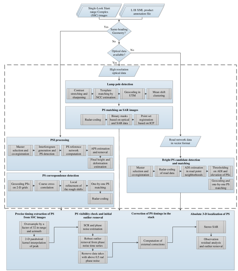
Figure 2: The flowchart of the automatic gcp generation algorithm. The input data is the Single-Look Slant range Complex (SLC) SAR images and their accompanying L1B product annotation files. The identical ps detection part is drawn inside the gray dashed rectangle. In case of ps detection from cross-heading viewing geometries, the algorithm receives as input the optical image or road network data of the scene upon availability. The processes are depicted with big blue rectangles while the sub-processes are shown with small gray rectangles. The name of each process step is written in bold letters. The last blue rectangle includes the processes and sub-processes that all the detected candidates should go through independent of the detection methodology.

The processing chain for automatic detection and positioning of gcps includes a set of procedures which starts from single-look slant range complex sar images and their corresponding product annotation files to absolute 3D coordinates of the chosen gcps. The flowchart of the algorithm is shown in Fig. 2. It consists of the following major processes which have to be carried out in the stated order:

1. identification of identical scatterers visible in multi-aspect sar images.

2. precise extraction of scatterers’ azimuth and range positions from sar images at sub-pixel level.

3. scatterer visibility check and initial removal of outliers from time series of phase noise.

4. correction of radar timings for all the perturbing signals.

5. estimation of the 3D absolute coordinates of the scatterers.

This section discusses each step. It is important to note that since some of the steps are well-established and well-documented techniques in the sar community, all the details will not be repeated here. Instead, for these processes, the relevant references are provided.

IV-A Identification of identical ps

This part has been already covered in Section III and is shown as the processes inside the gray dashed rectangle in the flowchart of Fig. 2. For detection of ps candidates from same-heading orbits, the psi processing is carried out following the guidelines from [24, 31, 32, 33] and the identical ps matching is done using the psi multitrack fusion algorithm described in [22, 23]. In the case of localization from cross-heading tracks, the ps candidate selection is carried out using the methods based on the optical data or on the road network data. Regardless of the detection method, the output of this step is the approximate radar coordinates of identical pss in terms of lines and samples in all non-coregistered images of different orbit tracks.

IV-B Precise extraction of ps timings

The rough radar coordinates of the pss from the previous step should be refined to sub-pixel level in order to extract the timings precisely. To this end, a process called pta is carried out [8]. In each image of the scene, a 32 $\times$ 32 window centered on the ps is extracted. In both range and azimuth direction, an oversampling by a factor of 32 is performed and the integer peak position of the ps response is measured. Subsequently in a 3 $\times$ 3 window centered on the peak position, a paraboloid interpolation is performed to refine the values around the maximum. This method allows the retrieval of the peak position of the ps with a sensitivity better than $\frac{1}{1000}$ of a pixel in each dimension [5]. These values are then converted to radar timings based on the product annotation files [25].

Based on the result of the pta for each ps, the refined peak power $P_{peak}$ and the clutter power $P_{clutter}$ can be computed. These values, if expressed in $dB$, are related to the scr of the target as:

$$\text{SCR}=10^{\big{(}\frac{P_{peak}-P_{clutter}}{10}\big{)}}$$ (9)

which is expressed as a digital number.

IV-C ps visibility check and initial outlier removal

The scr of potential ps candidates should be high enough in the stack of sar images so that the ps can be localized with high precision. Therefore, we analyze the time series of phase noise values $\bm{\sigma_{\phi}}$ of the pss to exclude potential outliers and check if the scatterer is visible in one data take or not. The $\sigma_{\phi}$ of a ps in acquisition $i$ is related to the scr of the target as [34]:

$$\sigma_{\phi_{i}}\approx\frac{1}{\sqrt{2~{}\text{SCR}_{i}}}~{}$$ (10)

which is expressed in radians. The values of $\bm{\sigma_{\phi}}$, for a specific ps in all data takes, are non-negative and follow a right-skewed distribution. Removal of outliers based on statistical measures such as mean or median is not recommended since many regular values can be categorized as outliers. Therefore, we use a method called adjusted boxplot which allows for robust elimination of outliers in univariate skewed distributions [35].

The main idea of the adjusted boxplot is to modify the original boxplot method, described in [36], to include information about the skewness of the data. Therefore, instead of classifying an observation as outlier if it lies outside of the interval defined by the boxplot method [36]:

$$\big{[}Q_{1}-1.5~{}IQR;~{}Q_{3}+1.5~{}IQR\big{]},$$ (11)

the adjusted boxplot method declares an observation as outlier if its value exceeds the following interval [35]:

$$\big{[}Q_{1}-1.5~{}e^{(-4MC)}~{}IQR;~{}Q_{3}+1.5~{}e^{(3MC)}~{}IQR\big{]}.$$ (12)

In (11), $Q_{1}$ and $Q_{3}$ are the first and the third quartiles of the data, respectively and $IQR=Q_{3}-Q_{1}$ denotes the interquartile range. In (12), $MC$ is the medcouple, a robust measure of the skewness of a univariate sample which for right-skewed distributions is always non-negative [37]. The exponential functions in (12) which depend on the $MC$ as well as the included coefficients are chosen experimentally based on some well-known skewed distributions. For more details on the theory and implementation of the adjusted boxplot method, the reader is referred to [35].

After the automatic identification and exclusion of $\sigma_{\phi}$ values which do not lie within the interval of (12), the remaining time series is analyzed to remove the data takes in which the specific ps is not visible. This is done by removing all $\sigma_{\phi}$ values which are above 0.5 radians ($\approx 30^{\circ}$) as is stated in [24].

IV-D Correction of ps timings in a stack

The correction of the extracted ps timings is performed using the imaging geodesy technique [1] which was briefly introduced in Subsection II-A. It is worth mentioning that the tropospheric and ionospheric effects are corrected based on global numerical weather models and global ionospheric maps, respectively, if local gnss receivers are not available in the vicinity of the investigated area. Along with these corrections comes the corresponding geometrical calibration of the sar sensor in range and azimuth which ensures centimeter localization accuracy. The calibration is based on corner reflectors with known reference coordinates [1]. The output of this part is the absolute 2D radar timing coordinates.

IV-E Absolute 3D localization of ps

At the final step in the processing chain, the corrected range and azimuth timings from the entire multi-aspect set of sar images are combined to retrieve the absolute 3D position of the ps with the stereo sar method described in Subsection II-A. Apart from the 3D position of the target, stereo sar reports on the standard deviation of each coordinate component ($S_{X}$, $S_{Y}$, $S_{Z}$) as the by-product of the least squares adjustment. Furthermore, observation quality of each ps i.e. the azimuth and range standard deviations ($S_{az}$, $S_{rg}$), retrieved from applying VCE to residuals, are delivered. It is important to note that the VCE is carried out individually for each geometry which allows to judge the consistency of the observed geometries with respect to the underlying assumption that the intersection occurs at a common ps.

The residuals of the adjusted range and azimuth observations are the basis for the elimination of outliers after stereo sar processing. Therefore, the processing is carried out repeatedly, where first the initial 3D coordinates are estimated using the provided input timings. The range and azimuth residuals are analyzed to exclude observations with residual values larger than 0.6 m in range or larger than 1.1 m in azimuth. The upper bounds correspond to the nominal spatial resolution of tsx high resolution spotlight products used in this study. Then stereo sar is performed again with the cleaned observations. This time, observations which show residuals larger than two times the $S_{az}$ and the $S_{rg}$ are removed. Additionally, to remove the pss which are not considered ideal for stereo sar due to wrong correspondence matching caused by several scatterers being too close, a third step of data cleaning is performed. pss having an $S_{az}$ higher than 20 cm in any of their azimuth geometries are removed based on the assumption that the discrepancy should not exceed the typical size of the ps object, for instance, a lamp pole.

The estimated variance-covariance matrix of the 3D position of the target is further used for error analysis. The matrix gives important information about the stability of the coordinates results and is affected by the factors stated in Subsection II-A.

V Experimental Results

In this section, the work-flow described in Section IV is applied on real data to produce remotely sensed sar-based gcps. In Subsection V-A, the results are reported for a small test site in Berlin where the detection of gcp candidates are carried out using cross-heading geometries. In Subsection V-B, the processing results are shown for the entire city of Oulu, Finland, where the detection and positioning are performed on ps candidates detected from both same- and cross-heading orbit tracks using the methods described in Subsections III-A and III-C, respectively.

V-A Berlin

The first test site includes a small area close to the Berlin central railway station. The sar data set, 214 images in total, consists of two stacks of tsx very high resolution spotlight images acquired with a range bandwidth of 300 MHz. The images cover a period of approximately six years from April 2010 to March 2015. In terms of viewing geometry, one stack was acquired from a descending orbit with images recorded at 05:20 coordinated universal time (UTC), and one stack was acquired from an ascending track with images recorded at 16:50 UTC. The acquisition parameters of each stack are summarized in Tab. I.

TABLE I: Acquisition parameters of stacks of sar images in Berlin

Beam Nr.	Incidence angle (degree)	Heading angle (degree)	Track type	Nr. of images
57	41.9	350.3	Asc	107
42	36.1	190.6	Dsc	107

For the selected test site, an aerial optical image with ground spacing of 7 cm is also available. The optical image is orthorectified and was used in a stereo matching process to produce a digital surface model with decimeter accuracy [38]. The optical image of the test site and the corresponding sar images are shown in Fig. 3.

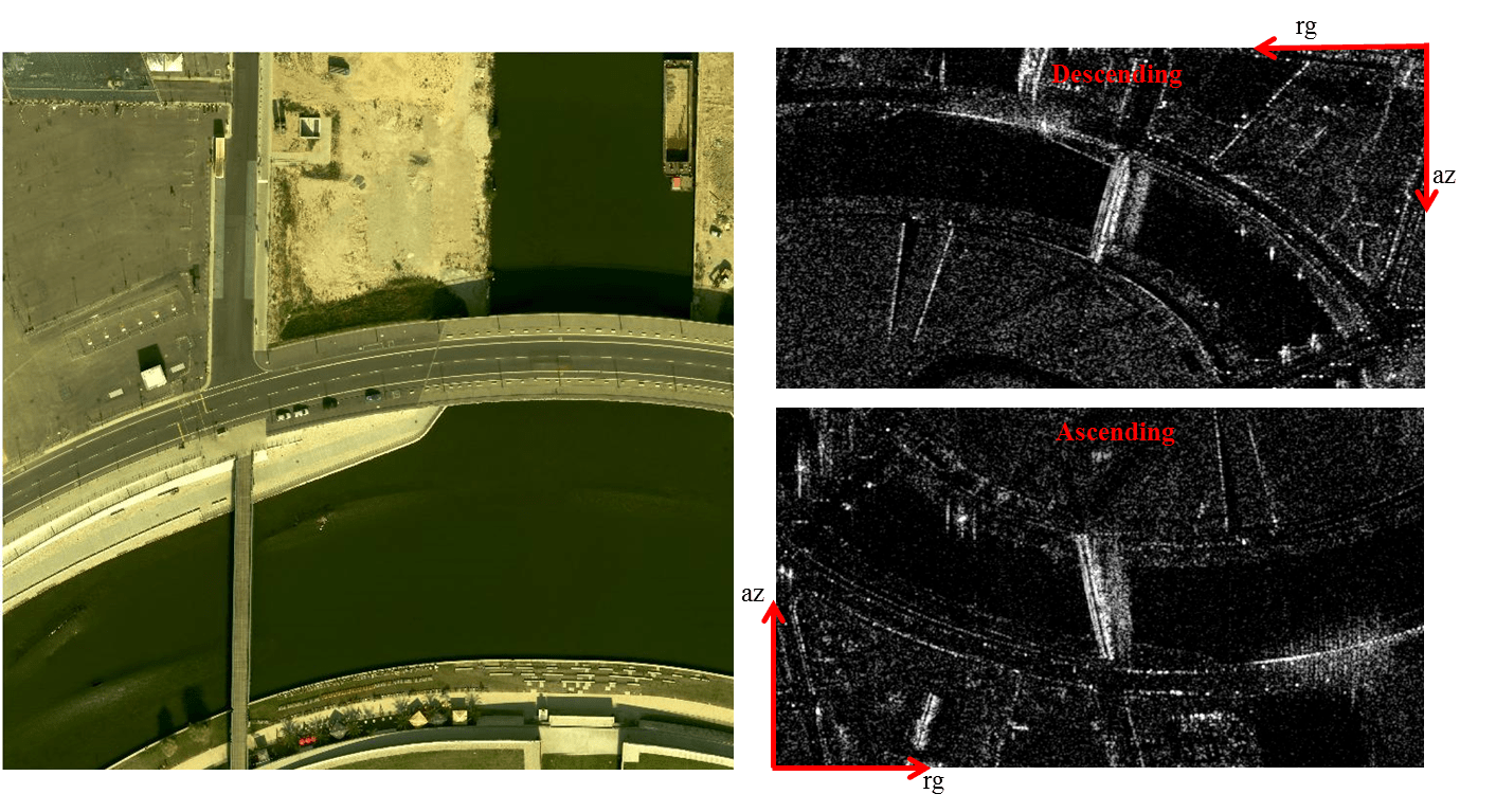
Figure 3: The optical image (left) and the sar amplitude images (right) of the test area in Berlin. The contrast of the optical image has been adjusted to illustrate the shadows of the lamp poles prominently.

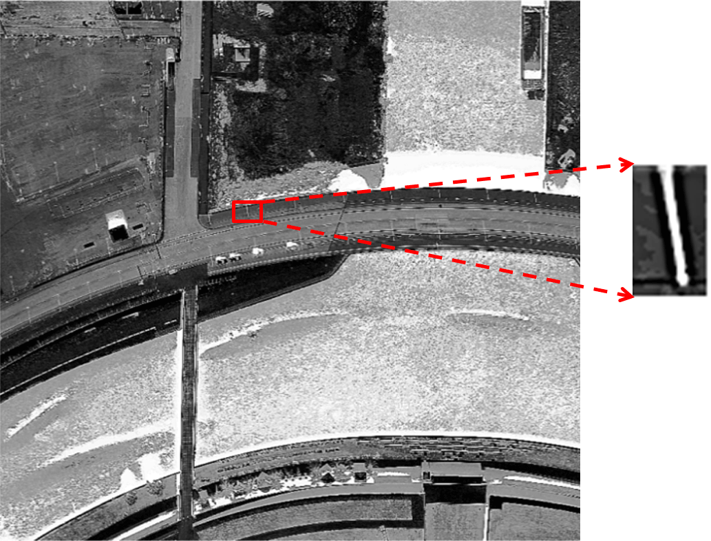
(a)

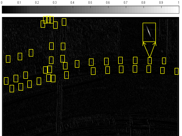
(b)

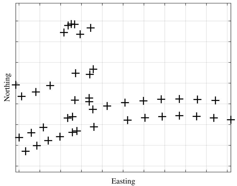
(c)

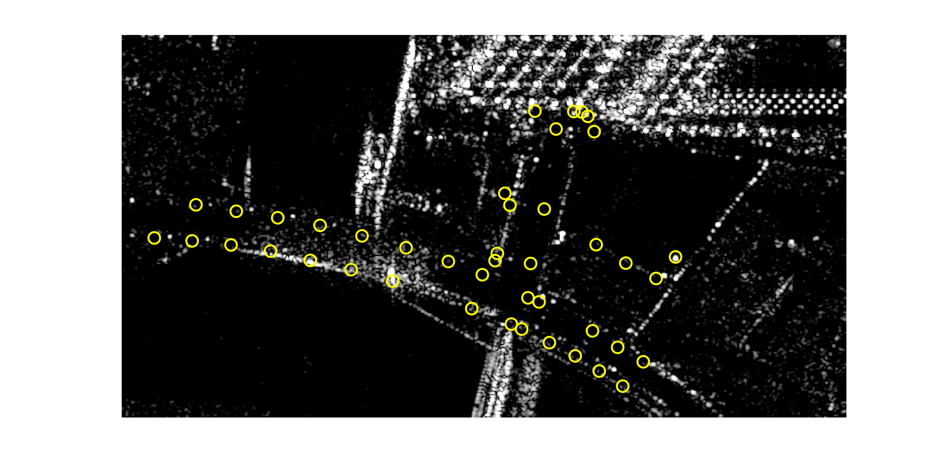
(d)

(e)

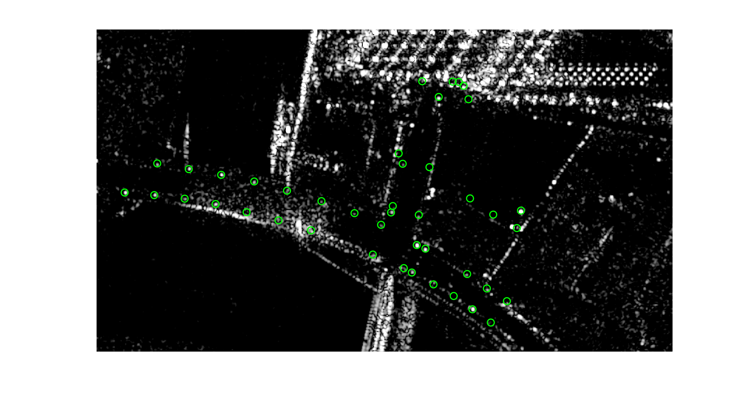
(f)

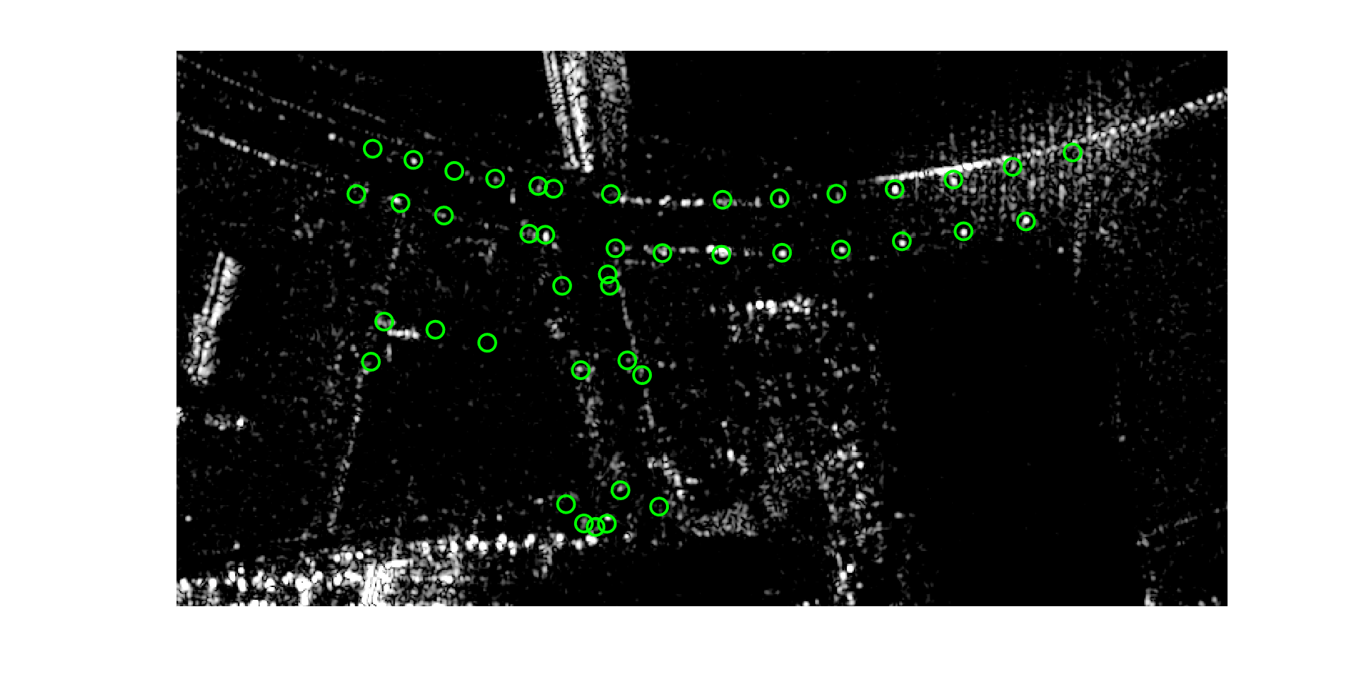
(g)

Figure 4: Demonstration of ps correspondence detection in Berlin based on high resolution optical data. (a) shows the pre-processed optical image after negative intensity transformation and the extracted template. (b) is the calculated ncc map after correlating the extracted lamp pole template with the reference image in which the detected objects are marked by yellow rectangles. (c) shows the 44 detected objects in the utm coordinate system after clustering. In (d) and (e), the radar-coded results are depicted by yellow circles which show offsets with respect to the bright points in the sar images. (f) and (g) show the results of matching after using the ICP algorithm on the descending and the ascending image, respectively. In the last two subfigures, it can be seen that the detected objects from the optical image (green circles) coincide with the visible bright points in the sar images.

The gcp candidate selection is carried out based on the optical data which includes the detection of lamp poles and their projection onto cross-heading sar images (see Subsection III-B). The individual steps of this process, applied on the Berlin test site, are shown in Fig. 4. After the extraction of the template (see Fig. 4(a)), the ncc map is calculated and pixels with values higher than 0.6 are classified as parts of shadows of lamp poles as illustrated in Fig. 4(b). It is important to note that the exact tuning of the threshold is not necessary as long as the value is chosen low enough. If the threshold is strictly chosen as a high value, although we are selecting the most similar pixels to the template, we may ignore all the other candidates which show less similarity to the template but might have been potential candidates for stereo SAR processing and 3D localization. Therefore, in our processing chain the default value is set to 0.6, which is slightly higher than the half of the ncc range [0,1], to guarantee a certain degree of similarity while selecting a large number of pixels. In the Berlin case study, this leads to the selection of 2030 pixels which are further clustered to represent the 44 detected objects in the utm coordinate system (see Fig. 4(c)). The objects include the lamp poles along the bridge and at the street perpendicular to the bridge as well as flag poles at the top left of the optical image close to the Berlin railway station. After radar-coding of the results onto the entire ascending and descending sar images, the mismatch between the projected points and the actual bright points in the sar images, depicted in Fig. 4(d) and Fig. 4(e), is resolved using ICP. The detection outcome is marked with green circles in Fig. 4(f) and Fig. 4(g). It is seen from the results that not all of the available street lights can be detected using the mentioned strategy as some can be occluded by cars or the object’s shadow is not distinctive enough to match the extracted template. However, this is of low importance in our application since in such a small test site, with an area less than two $\text{km}^{2}$, two or three gcps will certainly suffice. Moreover, if the method detects wrong candidates which do not fall in the category of pss, the subsequent pta and phase noise analysis will discard these points.

The precise radar timings of the pss are extracted using pta (see Subsection IV-B). Subsequently for each ps candidate in each data take, scr and $\sigma_{\phi}$ values are evaluated using (9) and (10), respectively. After excluding potential outliers with the adjusted boxplot method, the data takes in which the scatterer is not visible are discarded by thresholding on the $\sigma_{\phi}$ values (see Subsection IV-C). At this point, one might argue that analyzing the time series of the remaining $\sigma_{\phi}$ values can already give a hint if the scatterer is a suitable candidate for positioning or not. This statement is partially true since the mentioned analysis is only useful to separate the time-coherent scatterers from the non-coherent ones. It is possible that several scatterers, located close to each other, are mapped as one bright point which results in low $\sigma_{\phi}$ value but of course not a suitable candidate for stereo sar. These candidates are usually discarded in the stereo sar processing due to large $S_{az}$ values which indicate that not the same object has been detected from multiple viewing geometries. Therefore, in our processing chain, the detected candidates are not entirely removed based on their average scr and they are all passed to the final stereo sar processing.

As for the corrections, the ionospheric delay is estimated using global ionospheric maps. The tropospheric delay is estimated using the zenith path delay information of the closest permanent gnss station in Potsdam which is situated approximately 35 km away from the test site.

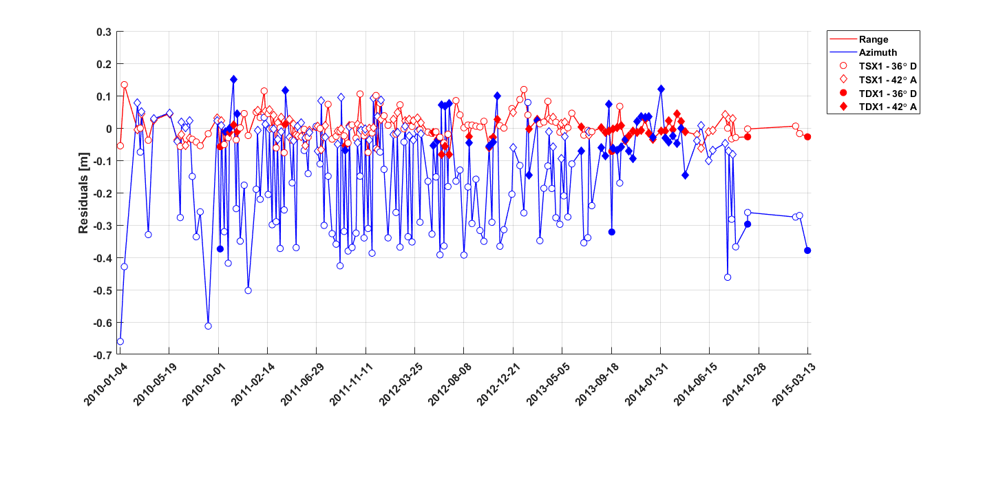
(a) $\text{PS}_{41}$

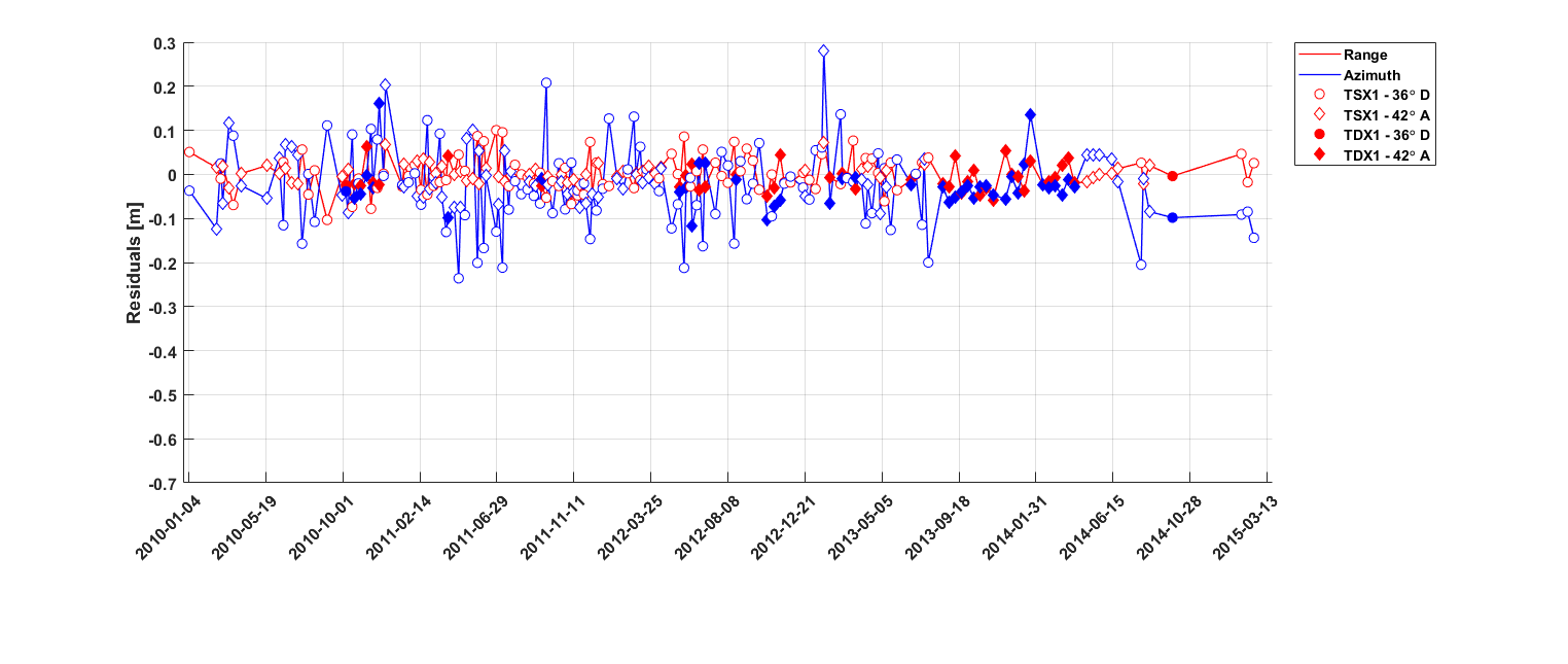
(b) $\text{PS}_{43}$

Figure 5: Range and azimuth residuals for two PS examples of the Berlin test case after the stereo sar processing. Step $1$ (gross outlier detection) and step $2$ ($2\sigma$ test) have already been applied.

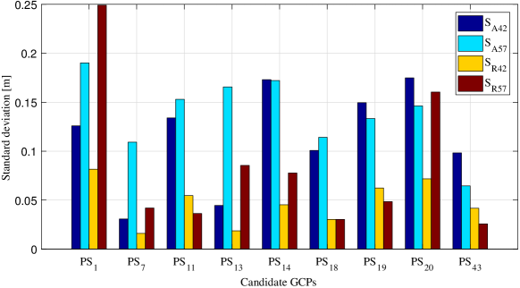
Figure 6: The posterior azimuth and range standard deviations ($S_{az}$, $S_{rg}$) of the 9 best gcp candidates estimated by VCE in the geodetic stereo sar processing.

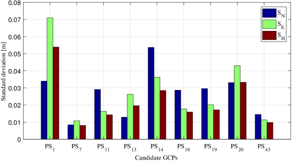
Figure 7: The posterior standard deviations scaled to 95$\%$ confidence level of the 9 best gcp candidates estimated posterior to the geodetic stereo SAR processing. The standard deviations are defined in the local coordinate system of Berlin in north, east and vertical direction ($S_{N}$, $S_{E}$, $S_{H}$).

The positioning of the 44 pss is carried out using stereo sar (see Subsection II-A) and is followed by outlier elimination according to criteria described in Subsection IV-E. Starting from the corrected input timings, the first solution is analyzed for gross outliers in the observations exceeding the resolution of the underlying tsx high-resolution spotlight product. Applying these thresholds to the residuals of the adjusted observations reduces the number of solvable pss from 44 to 42, because in the case of an obvious mismatch, all the observations of one geometry are removed. Moreover, the total number of observations is reduced by 25$\%$ but this strongly varies across the individual pss. After re-computation and application of the $2\sigma$ test using the estimated standard deviations from the VCE ($S_{az}$ , $S_{rg}$), the number of solvable pss remains 42 and the total amount of observations is reduced by another 8$\%$. At this stage, the data is fairly cleaned at the observation level regarding the individual range and azimuth geometries, but their consistency has not been considered so far. Looking at the observation residuals of the two pss displayed in Fig. 5 reveals that there are cases for which the azimuth of one geometry is clearly biased because we try to combine data from different phase centers. In the ideal case, the algorithm yields a coordinate solution for which all sets of observations (two sets of azimuth, two sets of range) can fulfill the range-Doppler positioning model of (3) and (4). For a mismatch or a spatial separation of the phase centers, the usually more precise range observations dominate the solution, and only one of the azimuth data sets may fit the estimated coordinates without a bias, but not the second set of azimuth data. Such a situation is illustrated by $\text{PS}_{41}$ (see Fig. 5(a)), where the $\text{36}^{\circ}$ azimuth displays a prominent bias of about -30 cm. To a certain degree this must be accepted since we can not expect ideal multi-directional pss, e.g. the lamp-poles have a certain diameter. In this study, as was mentioned in Subsection IV-E we define an empirical limit of 20 cm of what we consider acceptable which removes candidates like the $\text{PS}_{41}$ during the final processing step. Therefore, the residual results of scatterers like $\text{PS}_{43}$ (see Fig. 5(b)) may be seen as a best case scenario. The remaining difference in quality between range and azimuth is due to the non-square product resolution, i.e. the TS-X spotlight SLC data has a resolution of 0.6 m $\times$ 1.1 m in range and azimuth, respectively [25].

For the aforementioned reasons, only 9 pss remain which we consider as good gcp candidates. The bar graphs of Fig. 6 and Fig. 7 summarize the quality of these pss. Fig. 6 shows the posterior estimated standard deviations of observations. The $S_{az}$ values vary from 3 cm to 19 cm with an average of 12 cm while the $S_{rg}$ values range from 1 cm to 24 cm with an average of 6 cm. This indicates that, for these natural pss, the removal of error terms, as expressed in (1) and (2), and discarding the outliers allow sub-decimeter and decimeter precision in range and azimuth, respectively. In Fig. 7, the positioning quality is assessed by reporting the precision of the estimated coordinates. The standard deviations are defined in the local coordinate system of Berlin in north, east, and height ($S_{N}$, $S_{E}$, $S_{H}$) in the confidence level of 95$\%$. The mean values of $S_{N}$, $S_{E}$ and $S_{H}$ are 2.7 cm, 2.8 cm and 2.2 cm, respectively. The higher precision in the height direction is merely the effect of the cross-heading geometry used for the positioning.

Until now the discussion was mostly focused on analyzing the relative accuracy of the coordinates based on the posterior precision estimates. Although, the most reasonable procedure to validate the absolute accuracy is a point-wise comparison of stereo sar coordinates with respect to the corresponding gnss-surveyed ones, this was not applicable at the time of the study. Instead, the stereo sar estimated ellipsoidal heights of the 9 gcps were compared with the LiDAR heights of the same area. We assume the phase centers of the detected gcps are at the base of the lamp poles on the ground. Therefore, the cross-comparison includes finding the nearest neighbors of the gcp candidate in the LiDAR point cloud within the radius of 1 m, excluding the LiDAR points with large height values which originate from the top of the lamp pole, estimating the mode of the LiDAR heights to represent the reference height and evaluating the difference between the ellipsoidal height of stereo sar results with respect to the reference height. The radius of the neighborhood is chosen in a way that the reference height calculation includes a reasonable number of samples and still be small enough to possibly prevent the inclusion of different objects in the search window. It is also worth to note that the calculation of mode is carried out with the assumption that the majority of samples in the window stem from the ground. The results of the cross-comparison are reported in Tab. II. The estimated stereo sar and approximated LiDAR reference heights are denoted by ${\text{h}_{\text{S}}}$ and ${\text{h}_{\text{L}}}$ while their offset is represented by ${\text{h}_{\text{o}}}$. It is seen that for all except for one of the gcps the height offset is below 20 cm. The results report a bias of 13 cm and a precision of 5 cm overall with respect to the LiDAR data which roughly implies the absolute accuracy of the height estimation using the stereo sar method.

TABLE II: The result of cross-comparison between the estimated heights of stereo sar ${\text{h}_{\text{S}}}$ and their corresponding LiDAR heights ${\text{h}_{\text{L}}}$. The offset ${\text{h}_{\text{o}}}$ is an indicator for the absolute accuracy of ${\text{h}_{\text{S}}}$

GCP	${\text{h}_{\text{L}}}~{}\text{[m]}$	${\text{h}_{\text{S}}}~{}\text{[m]}$	${\text{h}_{\text{o}}}={\text{h}_{\text{S}}}-{\text{h}_{\text{L}}}~{}\text{[m]}$
${\text{PS}_{1}}$	74.64	74.80	0.16
${\text{PS}_{7}}$	74.45	74.54	0.09
${\text{PS}_{11}}$	74.83	74.99	0.16
${\text{PS}_{13}}$	75.40	75.62	0.22
${\text{PS}_{14}}$	73.87	73.96	0.09
${\text{PS}_{18}}$	73.87	73.95	0.08
${\text{PS}_{19}}$	75.59	75.76	0.17
${\text{PS}_{20}}$	75.02	75.18	0.16
${\text{PS}_{43}}$	79.78	79.85	0.07
Mean			$\mathbf{0.13}$
Standard deviation			$\mathbf{0.05}$

V-B Oulu

The second test site covers the entire city of Oulu. The sar data include four stacks of tsx high resolution spotlight products with 177 images in total. The images were acquired from May 2014 to October 2016, from two ascending orbits and two descending orbits. The acquisition parameters of the Oulu data set are reported in Tab. III while the mean scene coverage and the acquisition time plot of the tsx images are shown in Fig. 8. No images were ordered during the periods from November 2014 to March 2015 and November 2015 to March 2016 due to the accumulation of snow expected for Oulu during the winter months.

TABLE III: Acquisition parameters of stacks of sar images in Oulu

Beam Nr.	Incidence angle (degree)	Heading angle (degree)	Track type	Nr. of images
30	30.9	346.1	Asc	44
54	41.1	191.4	Dsc	44
69	46.2	350.0	Asc	38
94	53.4	187.5	Dsc	51

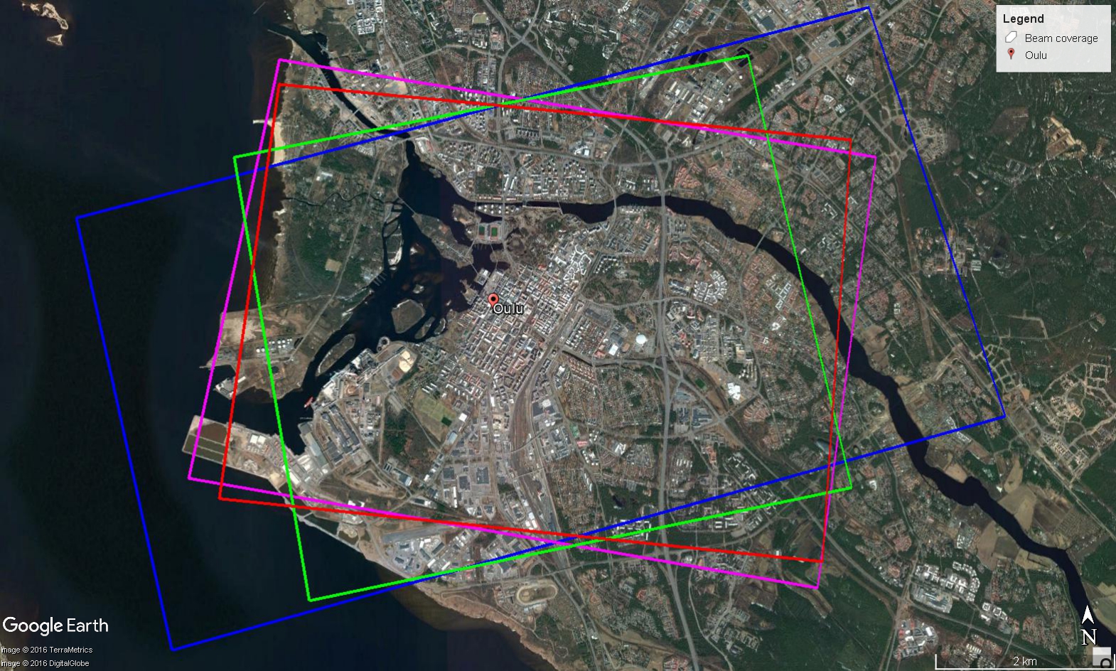
(a)

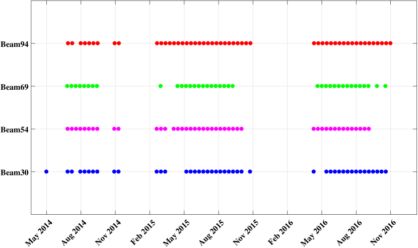
(b)

Figure 8: (a) The mean scene coverage of the tsx images overlaid on the optical image of Oulu taken from Google Earth. (b) The acquisition time plot of the tsx images of Oulu.

For Oulu, no optical images with sufficient spatial resolution were available for the detection of ps candidates from cross-heading geometries. Therefore, the road network data of Oulu was used instead. The data was freely accessed from the Finnish Transport Agency [39]. It was delivered in vector format in the utm coordinate system and includes the main streets and highways of Oulu.

The detection of ps candidates from the same-heading tracks was carried out using the multitrack psi fusion algorithm described in Subsection III-A. As the prerequisite of the algorithm, the psi processing was performed by the PSI-GENESIS of the German Aerospace Center (DLR) [33]. For each detected ps, the elevation and the deformation parameters (in this study only a linear trend) were estimated. As an example, the radar-coded ps elevation map of the ascending stack of beam 30 is visualized in Fig. 9. After geocoding, the 3D point clouds obtained from either ascending-ascending (AA) or descending-descending (DD) geometries form the initial input of the fusion algorithm as Fig. 10 demonstrates.

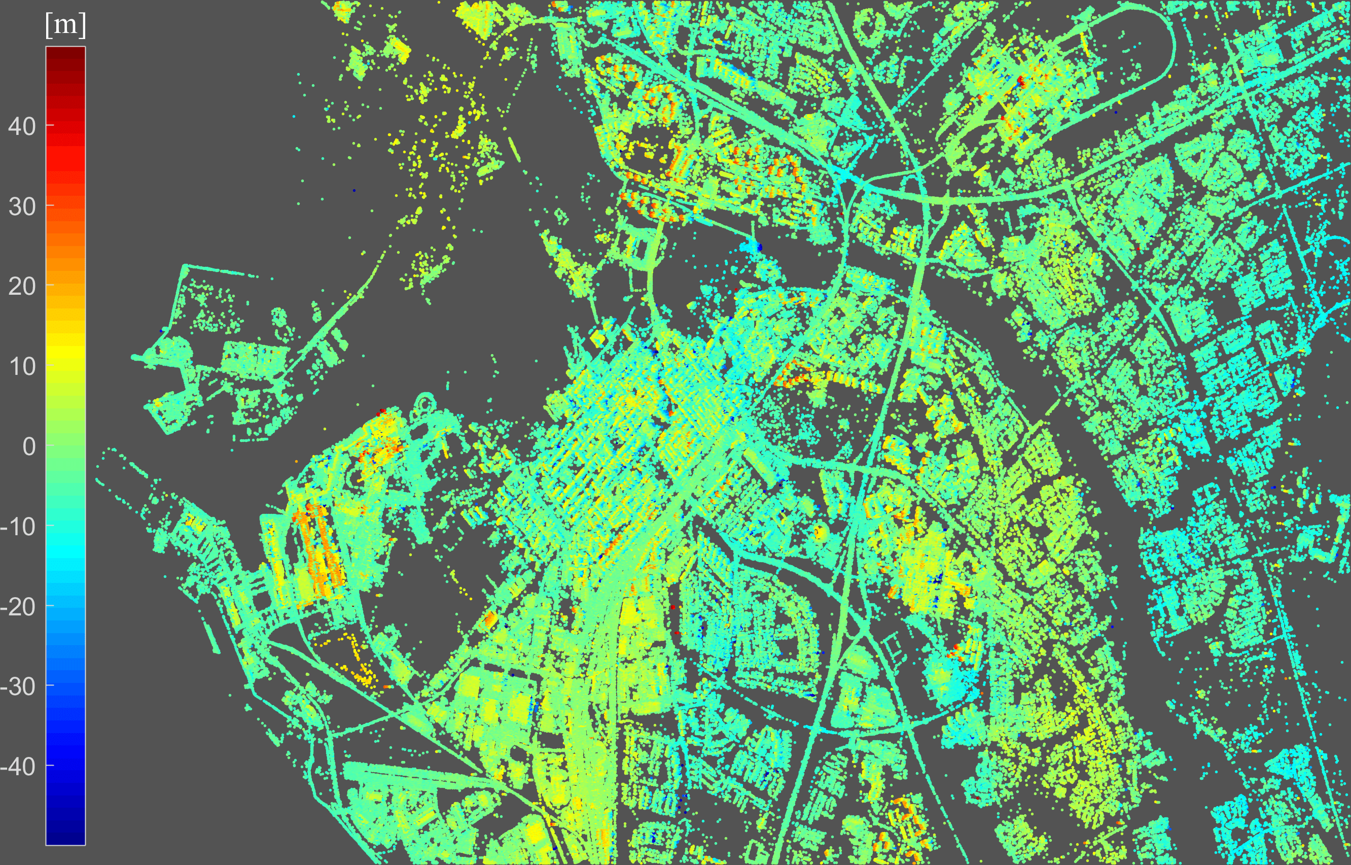
Figure 9: ps elevation map obtained from psi processing of an ascending stack of Oulu (beam 30). The total number of scatterers is approximately 540000 after selecting only the pss with posterior coherence values equal or higher than 0.7.

Fig. 10(a) shows the geocoded ps point clouds from the DD geometries, visualized in white and gray. The yellow points represent the identified ps pairs from the fusion algorithm. The total number of the correspondences is approximately 32000 and the Euclidean distances between the matched pss vary from 1.5 to 5 meters. In order to reduce the number of ps correspondences to the ones with higher quality and closer distance, as well as to preserve the homogeneity of the distribution, a regular grid was imposed on the point clouds. Inside the 10 m $\times$ 10 m grid, the ps pairs which were closer together and had lower adi values were selected to reduce the number of pairs from 32000 to 10000. The comparison between ps pairs before and after reduction can be seen in a zoomed-in area in Fig. 10(b) and Fig. 10(c), respectively. The same procedure depicted in Fig. 10 was also carried out for the sar images from the AA geometries and close to 9500 ps correspondences were detected. The results then were radar-coded for both geometry configurations.

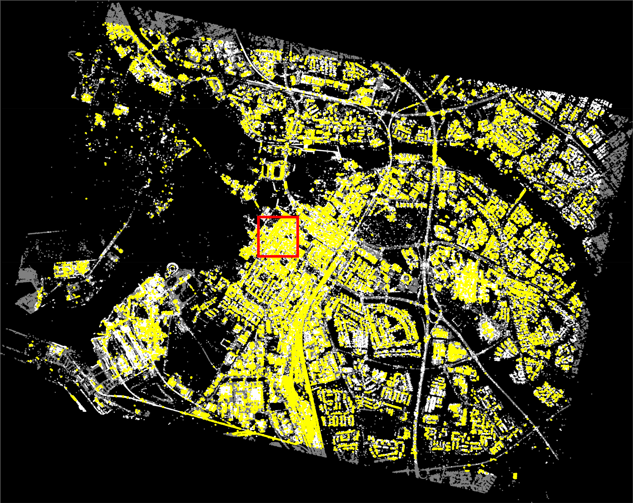
(a)

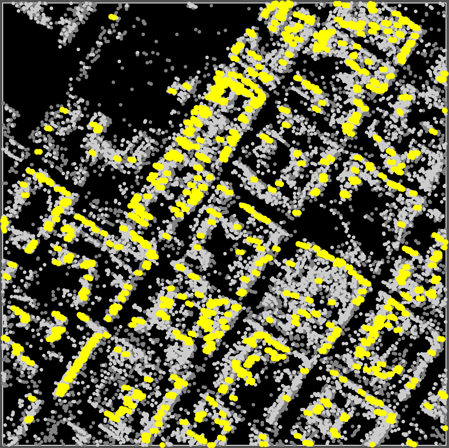
(b)

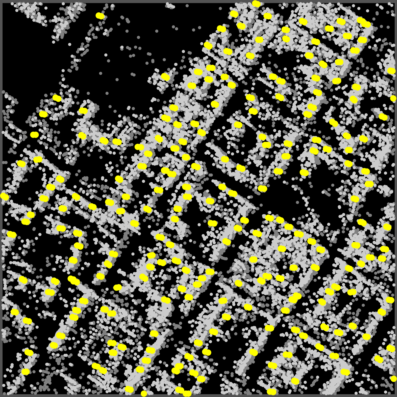
(c)

Figure 10: Depiction of ps correspondence detection from sar images of same-heading orbit tracks of Oulu using the first step of the multitrack ps fusion algorithm proposed in [22]. (a) shows the geocoded ps point clouds of beams 54 and 94 in a DD configuration as white and gray points as well as the detected ps correspondences in yellow. (b) and (c) show a zoom-in area of (a) marked by the red rectangle before and after imposing a 10 m grid in which the pairs with closest distance are chosen.

The ps candidates to be localized from the cross-heading geometries, either ascending-descending (AD) configuration or quad geometry (ADAD) configuration, were selected based on the detection of bright points along the roads using the road network data as was explained in Subsection III-C. The road network data was first radar-coded on the master scenes of all the four geometries as is seen on the mean intensity images of each stack in Fig. 11. A circular neighborhood with a radius of 70 pixels was then considered around each road network node within which the adi was evaluated for all pixels for all the four stacks. The neighborhood is chosen based on a rough knowledge on the maximum width of highways in Oulu ($\approx 35$ m) and was adapted to the sar data by taking into account the pixel spacing in range and azimuth direction and the oversampling factor used in the processing. After selecting the pixel with the lowest adi in each neighborhood, a further threshold of 0.25 on adi values, typically used in psi processing [31], selects the stable bright points from each stack. After geocoding, the pss from different stacks which are closer than a threshold of three meters are chosen as the final stereo candidates and are subsequently radar-coded on all the sar images. The distance threshold depends on the geometry configuration from which the user is interested to localize the targets. If same-heading geometries are considered the value should be lower than three meters in order to ensure correct ps correspondence detection. An example of ps candidates visible from ADAD configuration in Oulu is given in Fig. 12. The candidates are all assumed to be bases of lamp poles and can be seen as bright points inside the green circles. The explained procedure produced 107 and 52 initial candidates from ADAD and AD geometry configurations, respectively. The quantity is lower in the latter because of the strict distance threshold of 1.5 m imposed on coordinate differences of pss visible in different stacks. The threshold value is chosen empirically based on the histogram of minimum Euclidean distances evaluated between the PS pairs.

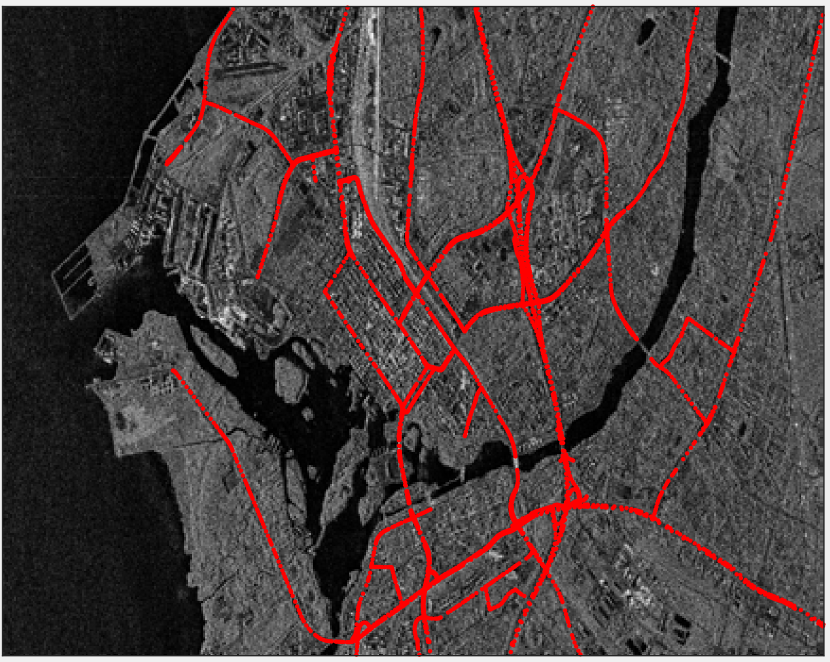
(a)

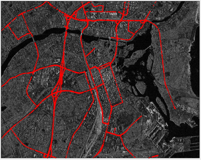
(b)

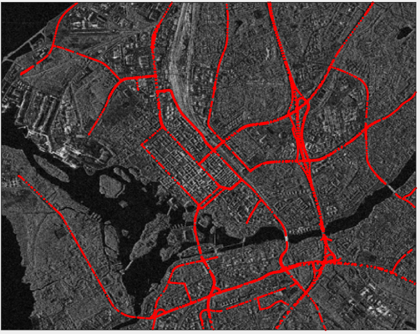
(c)

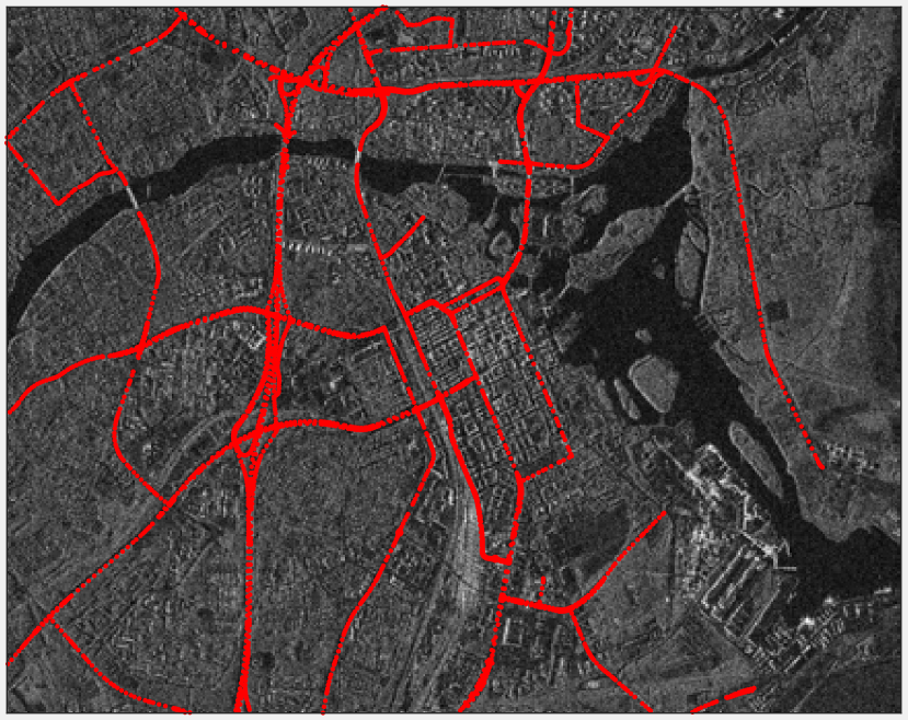
(d)

Figure 11: Projection of the road network data of Oulu onto the master scene of (a) beam 30, (b) beam 54, (c) beam 69 and (d) beam 94. The road data is represented by red points and is the basis for detection of identical ps candidates from cross-heading orbit geometries.

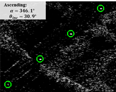
(a)

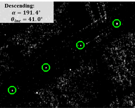
(b)

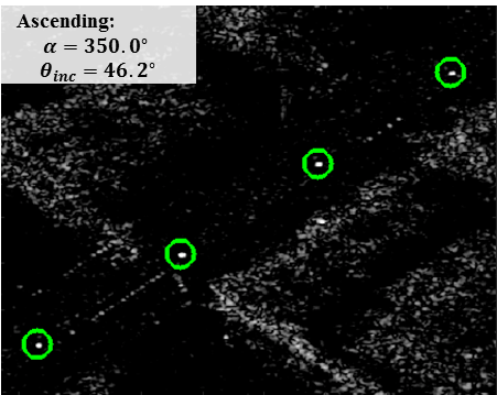
(c)

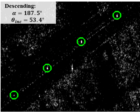
(d)

Figure 12: ps correspondence detection from ADAD geometry configuration. For each image, the respective averaged heading angle $\alpha$ and the averaged incidence angle $\theta_{inc}$ are stated.

The pta was performed on all the detected ps candidates in all the sar images in which the candidate was visible. For each candidate a time-series of $\bm{\sigma_{\phi}}$ was evaluated using (10). Fig. 13 demonstrates the initial outlier removal on two ps candidates based on the method of adjusted boxplot explained in Subsection IV-C. The $\sigma_{\phi}$ values of each scatterer are sorted in time in Fig.13a and Fig.13b. The distribution of $\bm{\sigma_{\phi}}$ is right-skewed in both cases as can be seen in Fig.13c and Fig.13d. From the distribution plots, one can detect the samples which are not connected to the tail of the distribution and mark them as potential outliers. This process is done automatically and without the need for manual intervention using the interval defined in (12). In Fig.13e and Fig.13f, the detected outliers are marked with red rectangles. For all the candidates the mentioned procedure was carried out.

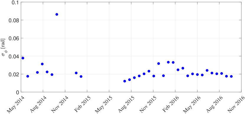
(a)

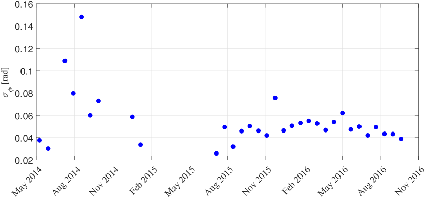
(b)

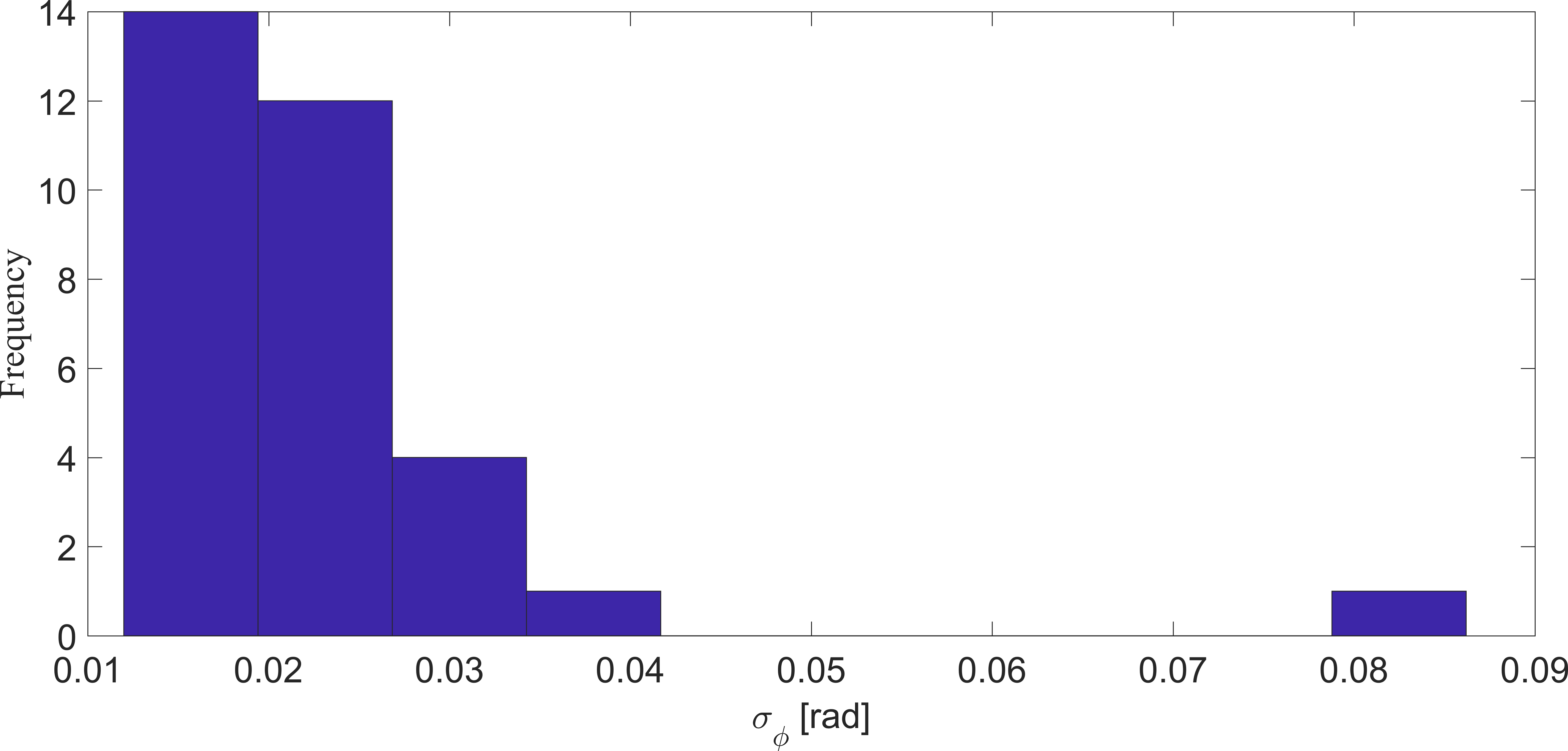
(c)

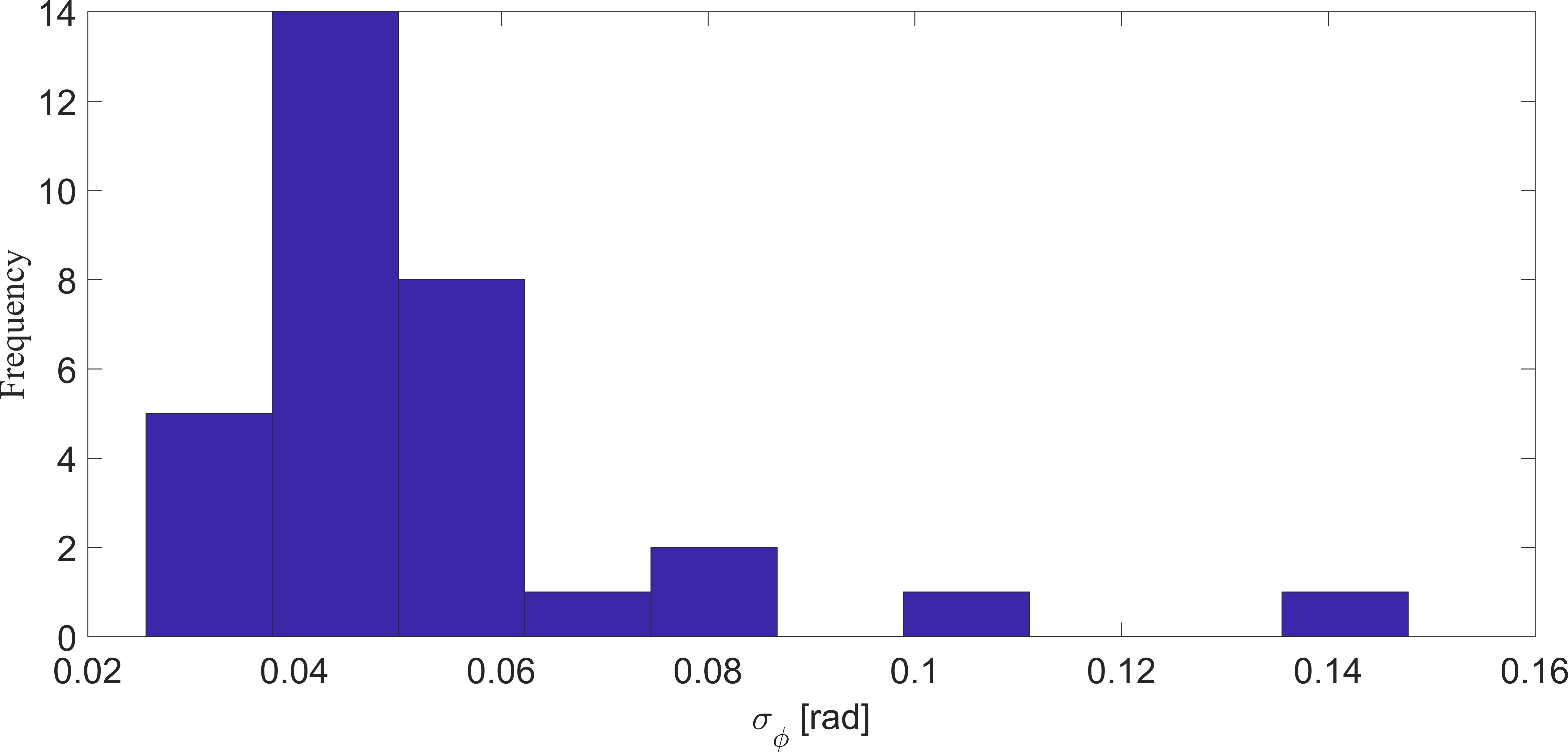
(d)

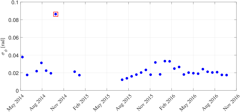
(e)

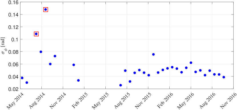
(f)

Figure 13: Example of initial outlier removal based on phase noise time series of the detected candidates. The outliers are identified and removed automatically based on the distribution of $\bm{\sigma_{\phi}}$.

The atmospheric corrections were carried out using global ionospheric maps and the global tropospheric zenith path delays provided with the Vienna mapping function [40] since there was no access to the Oulu gnss receiver at the time of the study. The geodynamic effects were fully considered according to the IERS conventions and all the effects were removed from the ps timings.

The final positioning was carried out by stereo sar with all the mentioned outlier removal steps in Subsection IV-E. The last criterion, which includes the removal of pss based on $S_{az}$ values higher than 20 cm, reduces the amount of total pss to only those points which can be considered ideal stereo candidates. The averaged quality of the estimated 3D coordinates for all the remaining high quality pss are reported in Tab. IV. The scatterers are categorized based on the geometry configuration that is used for their positioning. The results are all expressed in centimeter and are defined in the local east, north and vertical coordinates. The standard deviations are all defined within 95$\%$ confidence interval. From Tab. IV, it is seen that the averaged precisions are smaller than two decimeter for all the cases. As it was expected, the localization quality boosts as the difference in the viewing geometries becomes larger which is the case when changing from AA or DD to the AD and ADAD geometry configurations. It is also evident that for cross-heading geometries the retrieval of the height component is the most precise one as for the same-heading cases, the precision in the north component is the highest. Therefore, in general localization of targets from cross-heading tracks are desirable. The only remaining concern regarding localization using cross-heading tracks is the diameter of the lamp poles which may worsen the accuracy in the east coordinate component. This bias can be estimated and removed if the scatterer is also visible from same-heading tracks which is usually the case.

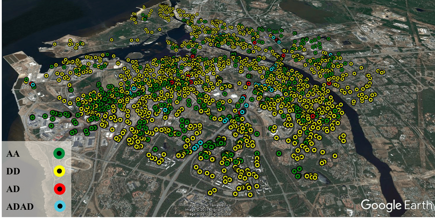
Figure 14: Total number of 2049 GCPs in Oulu color-coded based on the geometry configuration used for their positioning. The underlying optical image is taken from Google Earth.

TABLE IV: Averaged statistics based on the least squares estimated 3D coordinate standard deviations in Oulu. The letters A and D stand for ascending and descending geometries, respectively. The sample mean and standard deviation are denoted by $\mu$ and $\sigma$, and $S_{[ENH]}$ represent the local coordinates standard deviations within 95$\%$ confidence level

Geometry	Nr. Scatterers	$\mu_{\text{s}_{\text{E}}}~{}[\text{cm}]$	$\mu_{\text{s}_{\text{N}}}~{}[\text{cm}]$	$\mu_{\text{s}_{\text{H}}}~{}[\text{cm}]$	$\sigma_{\text{s}_{\text{E}}}~{}[\text{cm}]$	$\sigma_{\text{s}_{\text{N}}}~{}[\text{cm}]$	$\sigma_{\text{s}_{\text{H}}}~{}[\text{cm}]$
AA	565	17.73	5.04	15.87	11.98	2.63	11.09
DD	1417	15.08	3.80	16.71	10.38	2.10	11.30
AD	24	2.26	2.50	1.75	0.99	1.11	0.83
ADAD	43	1.17	1.40	1.12	0.42	0.55	0.37

The distribution of the total 2049 generated gcps is visualized on the optical image of Oulu in Google Earth in Fig. 14. The scatterers are color-coded based on the underlying geometry configuration used for their localization. It is seen that almost the entire area of Oulu is covered with the generated gcps. The ones from the same-heading geometries cover the built areas while the ones from cross-heading configuration include the base of lamp poles, street lights and traffic lights.

VI Summary, Conclusion and Outlook

In this paper we described a processing chain for automatic detection and positioning of opportunistic pss which are visible from multi-aspect tsx images. This paves the way for generation of gcps from sar data only.

Three algorithms have been recommended for identical PS detection which are different in terms of number of generated gcps and the subsequent positioning precision. The method based on the psi fusion algorithm is able to provide point correspondences even on buildings and areas with complex scattering mechanisms in sar images. Therefore, a large number of potential ps pairs can be obtained which normally cover the entire scene. The downside of the method is that sar image stacks are required for which a complete psi processing has to be performed separately before being able to find the ps correspondences. Furthermore, the method is usually applicable only for same-heading ps point clouds. Consequently in terms of localization precision with the subsequent stereo sar, the relative error in the cross-range is larger than the error for range and azimuth components. Another disadvantage is that many of the initial ps correspondences cannot be considered useful candidates for stereo sar and have to be eliminated later in the processing, because the registration is only performed within the limits of the psi 3D localization quality for which ps pairs with distances of up to five meters are detected. The detection algorithm based on external optical data is quite straightforward to implement and provides identical scatterers that are visible from cross-heading orbits leading to higher localization precision. The disadvantage of the method is that for reliable detection of lamp poles, the spatial resolution of the optical image should be in the sub-decimeter regime. Moreover, the method is highly prone to detecting other linear structures as shadows of lamp poles and therefore more sophisticated object detection algorithms are recommendable. The method based on vector road network data, similar to the optical method, provides candidates which are suitable to be localized from cross-heading geometries. Also the external data is freely accessible for most locations. The disadvantage of the method is that a co-registration on one master has to be carried out for each stack and the amplitude data must be calibrated.

It has been shown that the gcp generation processing chain is quite flexible as it allows the user to constraint the number and the quality of the candidate gcps either from the start of the procedure, by selecting different distance thresholds for detection or trimming the data based on estimated phase noise time series, or at the final step of the procedure based on the posterior quality indicators obtained from stereo sar.

By applying the algorithm to two test sites, it has been demonstrated that it is capable of positioning natural pss with precision values ranging from 2 cm and 4-5 cm, for cross-heading AD and ADAD configurations respectively, to approximately 20 cm for candidates extracted from same-heading geometries. As it was expected, the difference in the viewing geometries of the observed ps has the highest impact on the final localization precision followed by number of acquisitions used in stereo sar processing, the scr of the target and the quality of external error corrections. Furthermore, as a preliminary cross-comparison, the estimated ellipsoidal height of the retrieved candidates in Berlin were compared to the corresponding height of a LiDAR data which reported an average bias of approximately 13 cm.

The produced absolute gcps have ample of applications in geodesy and absolute mapping. These points may substitute the conventional gcps that are required for geo-referencing of satellite imagery which are usually surveyed at the field by gnss. They can be further integrated as absolute reference points into multi-pass insar techniques. Furthermore, they can be used to detect long-term ground motions with small magnitudes and low spatial frequency which are invisible to phase-based insar methods.

The future work will focus on smart pre-selection of the ps candidates by including the information obtained from pta, using integrated side-lobe ratio (ISLR), to robustly remove the ps candidates which are located too close to each other. Furthermore, the stereo sar processing could benefit from weighting the initial timing observations of the pss based on their respective scr or adi values and also can be carried out with robust parameter estimation schemes like M-estimator. Moreover, it is desirable to carry out gnss measurements at selected test sites to be able to correctly validate the absolute accuracy of the generated gcps. Finally, it is important to note that the proposed methodology is tailored to detection and absolute localization of gcps in urban area where a large number of pss are available. In applications where the investigated scene includes mainly non-urban area, it is recommendable to employ artificial pss such as corner reflectors or active transponders.

References

- [1] M. Eineder, C. Minet, P. Steigenberger, X. Y. Cong, and T. Fritz, “Imaging Geodesy - Toward Centimeter-Level Ranging Accuracy With TerraSAR-X,” IEEE Transactions on Geoscience and Remote Sensing, vol. 49, no. 2, pp. 661–671, Feb. 2011.
- [2] X. Y. Cong, U. Balss, M. Eineder, and T. Fritz, “Imaging Geodesy - Centimeter-Level Ranging Accuracy With TerraSAR-X: An Update,” IEEE Geoscience and Remote Sensing Letters, vol. 9, no. 5, pp. 948–952, Sep. 2012.
- [3] C. Gisinger, U. Balss, R. Pail, X. X. Zhu, S. Montazeri, S. Gernhardt, and M. Eineder, “Precise Three-Dimensional Stereo Localization of Corner Reflectors and Persistent Scatterers With TerraSAR-X,” IEEE Transactions on Geoscience and Remote Sensing, vol. 53, no. 4, pp. 1782–1802, Apr. 2015.
- [4] S. Hackel, O. Montenbruck, P. Steigenberger, U. Balss, C. Gisinger, and M. Eineder, “Model improvements and validation of TerraSAR-X precise orbit determination,” Journal of Geodesy, Dec. 2016.
- [5] U. Balss, X. Y. Cong, R. Brcic, M. Rexer, C. Minet, H. Breit, M. Eineder, and T. Fritz, “High precision measurement on the absolute localization accuracy of TerraSAR-X,” in Geoscience and Remote Sensing Symposium (IGARSS). IEEE, Jul. 2012, pp. 1625–1628.
- [6] U. Balss, C. Gisinger, X. Y. Cong, R. Brcic, S. Hackel, and M. Eineder, “Precise measurements on the absolute localization accuracy of TerraSAR-X on the base of far-distributed test sites,” in 10th European Conference on Synthetic Aperture Radar EUSAR, 2014.
- [7] U. Balss, H. Breit, T. Fritz, U. Steinbrecher, C. Gisinger, and M. Eineder, “Analysis of internal timings and clock rates of TerraSAR-X,” in Geoscience and Remote Sensing Symposium (IGARSS). IEEE, Jul. 2014, pp. 2671–2674.
- [8] I. G. Cumming and F. H.-c. Wong, Digital processing of synthetic aperture radar data: algorithms and implementation, ser. Artech House remote sensing library. Boston: Artech House, 2005.
- [9] H. Breit, E. Börner, J. Mittermayer, J. Holzner, and M. Eineder, “The TerraSAR-X Multi-Mode SAR Processor - Algorithms and Design,” in 5th European Conference on Synthetic Aperture Radar EUSAR, 2004.
- [10] C. Gisinger, “Atmospheric corrections for TerraSAR-X derived from GNSS observations,” Master Thesis, Technische Universität München, München, 2012.
- [11] G. Petit and B. Luzum, “IERS Conventions,” Verlag des Bundesamts für Kartographie und Geodäsie, Frankfurt am Main, IERS Technical Note No. 36, 2010.
- [12] M. Eineder, C. Gisinger, U. Balss, X. Y. Cong, S. Montazeri, S. Hackel, F. Rodriguez Gonzalez, and H. Runge, “SAR Imaging Geodesy– Recent Results for TerraSAR-X and for Sentinel-1,” in FRINGE 2017, 10th International Workshop on Advances in the Science and Applications of SAR Interferometry and Sentinel-1 InSAR, Jun. 2017.
- [13] C. Gisinger, S. Gernhardt, S. Auer, U. Balss, S. Hackel, R. Pail, and M. Eineder, “Absolute 4-D positioning of persistent scatterers with TerraSAR-X by applying geodetic stereo SAR,” in Geoscience and Remote Sensing Symposium (IGARSS). IEEE, Jul. 2015, pp. 2991–2994.
- [14] X. X. Zhu, S. Montazeri, C. Gisinger, R. F. Hanssen, and R. Bamler, “Geodetic SAR Tomography,” IEEE Transactions on Geoscience and Remote Sensing, vol. 54, no. 1, pp. 18–35, Jan. 2016.
- [15] S. Montazeri, X. X. Zhu, M. Eineder, and R. Bamler, “Three-Dimensional Deformation Monitoring of Urban Infrastructure by Tomographic SAR Using Multitrack TerraSAR-X Data Stacks,” IEEE Transactions on Geoscience and Remote Sensing, vol. 54, no. 12, pp. 6868–6878, Dec. 2016.
- [16] U. Balss, H. Runge, S. Suchandt, and X. Y. Cong, “Automated extraction of 3-D Ground Control Points from SAR images - an upcoming novel data product,” in Geoscience and Remote Sensing Symposium (IGARSS). IEEE, Jul. 2016, pp. 5023–5026.
- [17] D. O. Nitti, A. Morea, R. Nutricato, M. T. Chiaradia, C. La Mantia, L. Agrimano, and S. Samarelli, “Automatic GCP extraction with high resolution COSMO-SkyMed products,” in SAR Image Analysis, Modeling, and Techniques XVI, SPIE 10003, C. Notarnicola, S. Paloscia, N. Pierdicca, and E. Mitchard, Eds., Oct. 2016, p. 1000302.
- [18] P. Dheenathayalan, D. Small, A. Schubert, and R. F. Hanssen, “High-precision positioning of radar scatterers,” Journal of Geodesy, vol. 90, no. 5, pp. 403–422, May 2016.
- [19] S. Suri, P. Schwind, J. Uhl, and P. Reinartz, “Modifications in the SIFT operator for effective SAR image matching,” International Journal of Image and Data Fusion, vol. 1, no. 3, pp. 243–256, Sep. 2010.
- [20] D. G. Lowe, “Distinctive Image Features from Scale-Invariant Keypoints,” International Journal of Computer Vision, vol. 60, no. 2, pp. 91–110, Nov. 2004.
- [21] F. Dellinger, J. Delon, Y. Gousseau, J. Michel, and F. Tupin, “SAR-SIFT: A SIFT-Like Algorithm for SAR Images,” IEEE Transactions on Geoscience and Remote Sensing, vol. 53, no. 1, pp. 453–466, Jan. 2015.
- [22] S. Gernhardt, X. Y. Cong, M. Eineder, S. Hinz, and R. Bamler, “Geometrical Fusion of Multitrack PS Point Clouds,” IEEE Geoscience and Remote Sensing Letters, vol. 9, no. 1, pp. 38–42, Jan. 2012.
- [23] S. Gernhardt, “High Precision 3D Localization and Motion Analysis of Persistent Scatterers using Meter-Resolution Radar Satellite Data,” Doctoral Thesis, Technische Universität München, München, 2012.
- [24] B. M. Kampes, Radar Interferometry: Persistent Scatterer Technique. Dordrecht, the Netherlands: Springer, 2006.
- [25] T. Fritz and M. Eineder, “TerraSAR-X Ground Segment Basic Product Specification Document,” German Aerospace Center (DLR), Oberpfaffenhofen, Technical report, 2008.
- [26] S. Montazeri, X. X. Zhu, U. Balss, C. Gisinger, Y. Wang, M. Eineder, and R. Bamler, “SAR ground control point identification with the aid of high resolution optical data,” in Geoscience and Remote Sensing Symposium (IGARSS). IEEE, Jul. 2016, pp. 3205–3208.
- [27] R. C. Gonzalez and R. E. Woods, Digital image processing, 2nd ed. Upper Saddle River, N.J: Prentice Hall, 2002.
- [28] K. Briechle and U. D. Hanebeck, “Template matching using fast normalized cross correlation,” in Optical Pattern Recognition XII, SPIE 4387, D. P. Casasent and T.-H. Chao, Eds., Mar. 2001, pp. 95–102.
- [29] D. Comaniciu and P. Meer, “Mean shift: a robust approach toward feature space analysis,” IEEE Transactions on Pattern Analysis and Machine Intelligence, vol. 24, no. 5, pp. 603–619, May 2002.
- [30] P. Besl and N. D. McKay, “A method for registration of 3-D shapes,” IEEE Transactions on Pattern Analysis and Machine Intelligence, vol. 14, no. 2, pp. 239–256, Feb. 1992.
- [31] A. Ferretti, C. Prati, and F. Rocca, “Permanent scatterers in SAR interferometry,” IEEE Transactions on Geoscience and Remote Sensing, vol. 39, no. 1, pp. 8–20, Jan. 2001.
- [32] N. Adam, B. M. Kampes, M. Eineder, J. Worawattanamateekul, and M. Kircher, “The Development of a Scientific Permanent Scatterer System,” in Proceedings of the Joint ISPRS/EARSeL Workshop - High Resolution Mapping from Space 2003, Hannover, 2003.
- [33] N. Adam, F. R. Gonzalez, A. Parizzi, and R. Brcic, “Wide area Persistent Scatterer Interferometry: Current developments, algorithms and examples,” in Geoscience and Remote Sensing Symposium (IGARSS). IEEE, Jul. 2013, pp. 1857–1860.
- [34] N. Adam, B. M. Kampes, and M. Eineder, “The development of a scientific persistent scatterer system: Modifications for mixed ERS/ENVISAT time series,” in Proceedings of the Envisat ERS Symposium, Salzburg, Austria, 2004, pp. 1–9.
- [35] M. Hubert and E. Vandervieren, “An adjusted boxplot for skewed distributions,” Computational Statistics & Data Analysis, vol. 52, no. 12, pp. 5186–5201, Aug. 2008.
- [36] J. W. Tukey, Exploratory data analysis, ser. Addison-Wesley series in behavioral science. Reading, Mass: Addison-Wesley Pub. Co, 1977.
- [37] G. Brys, M. Hubert, and A. Struyf, “A Robust Measure of Skewness,” Journal of Computational and Graphical Statistics, vol. 13, no. 4, pp. 996–1017, Dec. 2004.
- [38] H. Hirschmuller, “Stereo Processing by Semiglobal Matching and Mutual Information,” IEEE Transactions on Pattern Analysis and Machine Intelligence, vol. 30, no. 2, pp. 328–341, Feb. 2008.
- [39] “Finnish Transport Agency,” Jan. 2017. [Online]. Available: http://www.liikennevirasto.fi/web/en
- [40] J. Boehm, B. Werl, and H. Schuh, “Troposphere mapping functions for GPS and very long baseline interferometry from European Centre for Medium-Range Weather Forecasts operational analysis data,” Journal of Geophysical Research: Solid Earth, vol. 111, no. B2, pp. 1–9, Feb. 2006.