How to distinguish between interacting and noninteracting molecules in tunnel junctions †
	Miguel A. Sierra,a David Sánchez,a Alvar R. Garriguesb, Enrique del Barcob, Lejia Wangc,d and Christian A. Nijhuisd,e
	Recent experiments demonstrate a temperature control of the electric conduction through a ferrocene-based molecular junction. Here we examine the results in view of determining means to distinguish between transport through single-particle molecular levels or via transport channels split by Coulomb repulsion. Both transport mechanisms are similar in molecular junctions given the similarities between molecular intralevel energies and the charging energy. We propose an experimentally testable way to identify the main transport process. By applying a magnetic field to the molecule, we observe that an interacting theory predicts a shift of the conductance resonances of the molecule whereas in the noninteracting case each resonance is split into two peaks. The interaction model works well in explaining our experimental results obtained in a ferrocene-based single-molecule junction, where the charge degeneracy peaks shift (but do not split) under the action of an applied 7-Tesla magnetic field. This method is useful for a proper characterization of the transport properties of molecular tunnel junctions.

1 Introduction

A molecular tunnel junction comprises molecules trapped between bulk metallic electrodes. These systems include electromigrated single-electron transistors ^{1, 2, 3, 4}, scanning tunneling microscopy break-junctions ^{5, 6}, and self-assembled monolayers of molecules ^{7, 8, 9, 10, 11, 12, 13, 14, 15, 16}. The energy spectrum of the molecule is characterized by both the highest occupied molecular orbital (HOMO) and the lower unoccupied molecular orbital (LUMO). When the HOMO or the LUMO aligns with the Fermi level of the leads $E_{F}$ within a certain tunnel broadening $\Gamma$, charge carriers can resonantly tunnel through the molecule ¹⁷. Tuning of the relative position of the molecular levels with respect to $E_{F}$ can be effectively achieved with a capacitively coupled gate electrode.

Since the level spacing between molecular levels $\Delta$ is typically large in molecular junctions, size quantization effects can be observed even at room temperature provided that $k_{B}T<\Delta$. However, the transport properties of the tunnel junction depend on $T$ because the electric current is a function of the electronic occupation at the leads, which is governed by a Fermi-Dirac distribution. The system response to both temperature and a bias voltage $V$ applied across the leads has been investigated in different classes of molecules: molecular diodes ^{11, 18, 19, 20}, molecular wires ^{21, 22, 23, 24, 25} and biomolecules^{26, 27, 28, 29}.

Due to the small size of molecules, in many occasions it is crucial to take into account an additional energy scale. In incoherent tunneling processes for molecules weakly coupled to the attached metals (i.e., for junction conductances smaller than $e^{2}/h$), charge carriers spend much time inside the molecule and Coulomb repulsion effects thus become relevant. This leads to regions with suppressed transport within the current–voltage characteristics of the molecular transistor (Coulomb blockade effect) ³⁰. Therefore, electrons flow through the molecule only when their energy is larger than the charging energy $U$. A key signature of Coulomb blockade is the appearance at $k_{B}T<U$ of areas of forbidden transport (commonly referred as “Coulomb diamonds") in the differential conductance curves as a function of source-drain and gate voltages. Coulomb blockade has been reported in molecular single-electron transistors ¹ as well as in different solid-state systems ^{34, 31, 32, 33}.

Garrigues et al. ⁴ have recently investigated the temperature dependence of charge transport across a ferrocene-based molecular transistor. They found that, when $T$ increases, the magnitude of the charge degeneracy points associated to current maxima decreases while the inverse behavior is observed for the current valleys. A noninteracting theoretical model that takes into account two single-particle levels in the molecule showed good agreement with the experimental data. Nevertheless, $\Delta$ and $U$ can be of the same order. Therefore, it is of fundamental importance to determine whether transport is due to noninteracting (independent electrons) or interacting (Coulomb blockade) physics. In this work, we demonstrate that an interacting theoretical model can equally well fit the experimental results and hence offer an alternative explanation for the results found in Ref. ⁴.

Our finding promptly triggers the following interesting question: How could one distinguish between both transport mechanisms (noninteracting case and Coulomb blockade) in a particular molecular junction setup? We stress that this question is unique to molecular devices since quantum dot systems exhibit charging energies much larger than the mean level spacing ³⁴. In molecular tunnel junctions, the level spacing is comparable to the charging energy, making it difficult to differentiate between the two cases. Here, we suggest that an externally applied magnetic field would serve as a tool to discern between the two transport mechanisms. Our proposal is illustrated in Fig. 1. In the top panel we depict a molecule with two single-particle quantum levels ($\varepsilon_{1}$ and $\varepsilon_{2}$) coupled to two electrodes ($L$ and $R$). The linear conductance would then show two peaks that are spin-split under the action of a magnetic field (top-right panel). The interacting counterpart is sketched in the lower panel where we consider one quantum level $\varepsilon_{1}$ and charging energy $U$. Due to Coulomb repulsion induced splitting, two conductance peaks are expected at zero magnetic field (bottom-right panel). Yet, with increasing magnetic field each resonance is not split but shifts in energy as shown. The differing current response would allow us to characterize the precise transport mechanism in a given molecular tunnel junction. Below, we support this proposal with a nonequilibrium Green function based calculation that agrees with the experimentally observed conductance peaks of a ferrocene-based molecular tunnel junction in the presence of magnetic fields.

2 Theoretical framework

Consider a single molecule coupled to the left, $L$, and right, $R$, metallic electrodes via tunneling barriers. We model the system with the single-impurity Anderson Hamiltonian,

$$\mathcal{H}=\mathcal{H}_{\rm mol}+\mathcal{H}_{\rm leads}+\mathcal{H}_{\rm tunnel}\,.$$ (1)

First, $\mathcal{H}_{\rm mol}$ describes the electrons in the molecule. For definiteness, we focus on the $N$-th molecular resonance. Its total energy $E$ is given by the sum of a kinetic part ($\varepsilon_{N}$) and a potential term. The latter originates from the interaction with the surrounding electrodes (source, drain and gate $g$ terminals). Following standard electrostatics, we model the coupling between the molecule and the electrodes with capacitances $C_{L}$, $C_{R}$ and $C_{g}$ (constant interaction model). Let $\mu_{m}(N)=E(N)-E(N-1)$ be the molecular electrochemical potential. Then,

$$\mu_{m}(N)=\frac{(2N-1)e^{2}}{2C}-e\frac{C_{L}V_{L}+C_{R}V_{L}+C_{g}V_{g}}{C}+\varepsilon_{N}\,,$$ (2)

($C=C_{L}+C_{R}+C_{g}$ is the total capacitance). Calculation of $\mu_{m}(N)$ is important because it determines the molecule’s addition energy, $\Delta\mu(N)=\mu_{m}(N+1)-\mu_{m}(N)$. It is straightforward to see that $\Delta\mu_{m}(N)=\Delta_{N}+e^{2}/C$, where $\Delta_{N}=\varepsilon_{N+1}-\varepsilon_{N}$. For the moment, we consider the spin-degenerate case (we will later discuss magnetic field effects). Then, $\varepsilon_{N+1}=\varepsilon_{N}$ and the resonance spacing is entirely given by the charging energy $U=e^{2}/C$. As a consequence, we can write

$$\mathcal{H}_{\rm mol}=\sum_{\sigma}\varepsilon_{m}d^{\dagger}_{\sigma}d_{\sigma}+Ud_{\uparrow}^{\dagger}d_{\uparrow}d_{\downarrow}^{\dagger}d_{\downarrow}\,,$$ (3)

where $\varepsilon_{m}=\varepsilon_{N}-e(C_{L}V_{L}+C_{R}V_{L}+C_{g}V_{g})/C$ is the single-particle energy including possible level renormalizations due to polarization effects. In Eq. (3) $d_{\sigma}^{\dagger}$ ($d_{\sigma}$) is the creation (annihilation) operator for electrons in the localized level and $\sigma=\{\uparrow,\downarrow\}$.

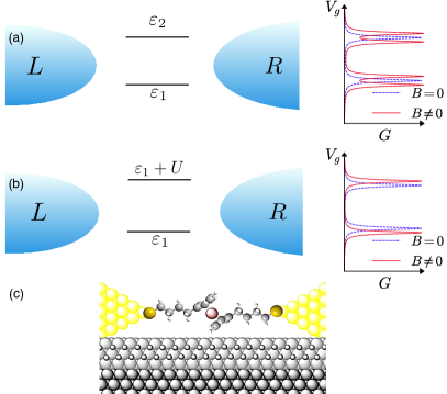
Fig.  1: Sketch of our proposal on how to evaluate the importance of electron-electron interactions in transport through molecules sandwiched between left ($L$) and right ($R$) metallic electrodes (tunnel junction). (a) The noninteracting case considers two molecular levels $\varepsilon_{1}$ and $\varepsilon_{2}$, which yield two conductance resonances as shown in the right plot (dashed blue lines). (b) The interacting case encompasses a single level $\varepsilon_{1}$ and a charging energy $U$, which also give rise to two conductance peaks. Remarkably, when a magnetic field $B$ is turned on the noninteracting resonances split as $B$ increases (red curves) whilst the interacting peaks shift. This different magnetic response allows us to characterize the transport mechanism in molecular tunnel junctions. (c) Schematic of the S-(CH₂)₄-ferrocenyl-(CH₂)₄-S molecular tunnel junction used to test our proposal.

The metallic electrodes are represented in Eq. (1) by

$$\mathcal{H}_{\rm leads}=\sum_{\alpha k\sigma}\varepsilon_{\alpha k}c_{\alpha k\sigma}^{\dagger}c_{\alpha k\sigma}\,,$$ (4)

where $\alpha=L,R$ and $c_{\alpha k\sigma}^{\dagger}$ ($c_{\alpha k\sigma}$) is the creation (annihilation) of conduction electrons with energy spectrum $\varepsilon_{\alpha k}$ ($k$ is the wave number).

Finally, the coupling of the molecule to the electrodes in Eq. (1) is described by the tunnel Hamiltonian

$$\mathcal{H}_{\rm tunnel}=\sum_{\alpha k\sigma}t_{\alpha k}c^{\dagger}_{\alpha k\sigma}d_{\sigma}+{\rm h.c.}\,,$$ (5)

where $t_{\alpha k}$ is the electronic tunnel amplitude.

3 Electric current

The current can be found from the time evolution of the expected value of the occupation in one of the electrodes: $I_{\alpha}=-ed\langle n_{\alpha}(t)\rangle/dt$, where $n_{\alpha}=c_{\alpha k\sigma}^{\dagger}c_{\alpha k\sigma}$. Due to charge conservation in the steady state, one has $I_{L}+I_{R}=0$ and this implies that current can be calculated in one of the electrodes only: $I\equiv I_{L}$. Applying the Keldysh-Green’s function formalism ³⁸, the electric current in terms of the transmission function $\mathcal{T}(\omega)$ becomes

$$I=\frac{e}{h}\int_{-\infty}^{\infty}d\omega\mathcal{T}(\omega)[f_{L}(\omega)-f_{R}(\omega)]\,,$$ (6)

with $f_{\alpha}(\omega)=1/[\exp{(\omega-\mu_{\alpha})/k_{B}T}+1]$ the leads’ Fermi-Dirac distribution with electrochemical potentials $\mu_{L}=\varepsilon_{F}+eV/2$ and $\mu_{R}=\varepsilon_{F}-eV/2$. The transmission obeys the expression

$$\mathcal{T}(\omega)=\sum_{\sigma}{\Gamma}_{L}{\Gamma}_{R}G^{r}_{\sigma,\sigma}G^{a}_{\sigma,\sigma}\,,$$ (7)

where $\Gamma_{\alpha}(\omega)=2\pi\rho_{\alpha}|t_{\alpha k}|^{2}$ is the tunnel hybridization due to coupling with electrode $\alpha$ ($\rho_{\alpha}$ is the density of states for electrode $\alpha$). The total broadening is then $\Gamma=\Gamma_{L}+\Gamma_{R}$. Quite generally, $\Gamma$ is a function of energy $\omega$ because electron tunneling depends on the position of each molecular level via the tunnel barrier height. This is important for the fit of the experimental curves, as we will discuss below.

In Eq. (7), $G^{r}_{\sigma,\sigma}(\omega)$ and $G^{a}_{\sigma,\sigma}(\omega)$ are the Fourier transforms for the retarded and advanced Green’s function, respectively, of the molecular system,

$$G^{r}_{\sigma,\sigma}(t,t^{\prime})=-\frac{i}{\hbar}\theta(t-t^{\prime})\langle[d_{\sigma}(t),d_{\sigma}^{\dagger}(t^{\prime})]_{+}\rangle\,,$$ (8)

where $\theta(t-t^{\prime})$ is the Heaviside function and $[\cdots]_{+}$ denotes the anticommutator.

4 Green’s function

In this work we use an approximate expression that works fairly well for the Coulomb blockade regime. This regime is characterized by strong electron-electron interactions and weak couplings to the electrodes ($U>k_{B}T>\Gamma_{\alpha}$). Temperature is moderate such that Kondo correlations can be safely neglected. This amounts to disregarding both the charge excitation correlators $\mathopen{\hbox{\set@color${\langle}$}\kern-1.94444pt\leavevmode\hbox{\set@color${\langle}$}}d_{\sigma}d_{\bar{\sigma}}^{\dagger}C_{\alpha k\bar{\sigma}},d_{\sigma}^{\dagger}\mathclose{\hbox{\set@color${\rangle}$}\kern-1.94444pt\leavevmode\hbox{\set@color${\rangle}$}}$, $\mathopen{\hbox{\set@color${\langle}$}\kern-1.94444pt\leavevmode\hbox{\set@color${\langle}$}}d_{\sigma}C_{\alpha k\bar{\sigma}}^{\dagger}d_{\bar{\sigma}},d_{\sigma}^{\dagger}\mathclose{\hbox{\set@color${\rangle}$}\kern-1.94444pt\leavevmode\hbox{\set@color${\rangle}$}}$ and $\mathopen{\hbox{\set@color${\langle}$}\kern-1.94444pt\leavevmode\hbox{\set@color${\langle}$}}C_{\alpha k\sigma}d_{\bar{\sigma}}^{\dagger}C_{\alpha k\bar{\sigma}},d_{\sigma}^{\dagger}\mathclose{\hbox{\set@color${\rangle}$}\kern-1.94444pt\leavevmode\hbox{\set@color${\rangle}$}}$, and the spin correlator $\mathopen{\hbox{\set@color${\langle}$}\kern-1.94444pt\leavevmode\hbox{\set@color${\langle}$}}C_{\alpha k\sigma}C_{\alpha k\bar{\sigma}}^{\dagger}d_{\bar{\sigma}},d_{\sigma}^{\dagger}\mathclose{\hbox{\set@color${\rangle}$}\kern-1.94444pt\leavevmode\hbox{\set@color${\rangle}$}}$. Then, the equation-of-motion technique ³⁹ leads to the following system of equations in the Fourier space

$$(\omega-\varepsilon_{m})G^{r}_{\sigma,\sigma} =1+\sum_{\alpha k}t_{\alpha k}^{*}G^{r}_{\alpha k\sigma,\sigma}+U\mathopen{\hbox{\set@color${\langle}$}\kern-1.94444pt\leavevmode\hbox{\set@color${\langle}$}}d_{\sigma}n_{\bar{\sigma}},d_{\sigma}^{\dagger}\mathclose{\hbox{\set@color${\rangle}$}\kern-1.94444pt\leavevmode\hbox{\set@color${\rangle}$}}\,,$$ (9)

$$(\omega-\varepsilon_{m}-U)\mathopen{\hbox{\set@color${\langle}$}\kern-1.94444pt\leavevmode\hbox{\set@color${\langle}$}}d_{\sigma}n_{\bar{\sigma}},d_{\sigma}^{\dagger}\mathclose{\hbox{\set@color${\rangle}$}\kern-1.94444pt\leavevmode\hbox{\set@color${\rangle}$}} =\langle n_{\bar{\sigma}}\rangle+\sum_{\alpha k}t_{\alpha k}^{*}\mathopen{\hbox{\set@color${\langle}$}\kern-1.94444pt\leavevmode\hbox{\set@color${\langle}$}}C_{\alpha k\sigma}n_{\bar{\sigma}},d_{\sigma}^{\dagger}\mathclose{\hbox{\set@color${\rangle}$}\kern-1.94444pt\leavevmode\hbox{\set@color${\rangle}$}}\,,$$ (10)

$$(\omega-\varepsilon_{\alpha k})\mathopen{\hbox{\set@color${\langle}$}\kern-1.94444pt\leavevmode\hbox{\set@color${\langle}$}}C_{\alpha k\sigma}n_{\bar{\sigma}},d_{\sigma}^{\dagger}\mathclose{\hbox{\set@color${\rangle}$}\kern-1.94444pt\leavevmode\hbox{\set@color${\rangle}$}} =t_{\alpha k}\mathopen{\hbox{\set@color${\langle}$}\kern-1.94444pt\leavevmode\hbox{\set@color${\langle}$}}d_{\sigma}n_{\bar{\sigma}},d_{\sigma}^{\dagger}\mathclose{\hbox{\set@color${\rangle}$}\kern-1.94444pt\leavevmode\hbox{\set@color${\rangle}$}}\,,$$ (11)

which can be readily solved for the retarded Green’s function

$$G^{r}_{\sigma,\sigma}(\omega)=\frac{1-\langle n_{\bar{\sigma}}\rangle}{\omega-\varepsilon_{m}-\Sigma}+\frac{\langle n_{\bar{\sigma}}\rangle}{\omega-\varepsilon_{m}-U-\Sigma}\,,$$ (12)

where $\Sigma\simeq-i\Gamma/2$ and the mean occupation $\langle n_{\bar{\sigma}}\rangle$ of the molecular level is evaluated from

$$\langle n_{\sigma}\rangle=\int d\omega\frac{\Gamma_{L}f_{L}(\omega)+\Gamma_{R}f_{R}(\omega)}{\Gamma}\rho_{\sigma}(\omega)\,.$$ (13)

$\rho_{\sigma}(\omega)=-(1/\pi)\text{Im}{[G^{r}_{\sigma,\sigma}]}$ is the molecular level spectral function.

Interestingly, the Green’s function in Eq. (12) shows two poles despite the fact that we are considering a single molecular level. These two poles will be resolved in a transport experiment when $U$ is larger than $\Gamma$, which is the typical situation for weakly coupled molecules. Equation (12) is also capable of describing a strongly coupled molecule (i.e., when $\Gamma\gg U$), in which case the molecule effectively acts as a noninteracting channel. Therefore, our equation-of-motion model encompasses a broad variety of situations provided Kondo physics is not important.

Therefore, in the Coulomb blockade regime ($U\gg\Gamma$) we expect two resonances in the transmission function separated by the charging energy $U$. This situation resembles very much the case of two molecular levels $\varepsilon_{1}$ and $\varepsilon_{2}$ (e.g., HOMO and LUMO) used in Ref. ⁴. In fact, the transmission function for two noninteracting levels is given by the sum of two Breit-Wigner (Lorentzian) line shapes ($i=1,2$),

$$\mathcal{T}(\omega)=\sum_{i}\frac{\gamma_{Li}\gamma_{Ri}}{(\omega-\varepsilon_{i})^{2}+\gamma_{i}^{2}/4}\,,$$ (14)

which also gives rise to two resonances like Eq. (12). For that reason, it is difficult to tell whether interactions will play a significant role in the electronic transport through molecules with level spacings $|\varepsilon_{2}-\varepsilon_{1}|$ of the same order as $U$. We will below demonstrate that an external magnetic field helps solve this critical issue.

5 Results

The self-consistent calculation of Eqs. (12) and (13) completely determines the transmission given by Eq. (7). We will now show that this solution nicely fits the experimental results of Ref. ⁴.

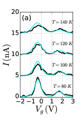
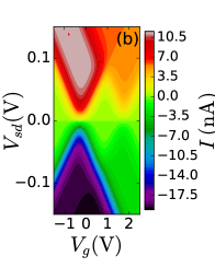
Fig.  2: (a) Current $I$ as a function of the gate voltage $V_{g}$ for different values of the indicated temperatures and a source-drain voltage $V=10$ mV. Experimental (theoretical) results are depicted with black (blue) curves (experimental data is extracted from Ref. ⁴). Curves for different temperature are shifted vertically for the sake of clarity (offset: $5$ nA). (b) Calculated current at $T=80$ K as a function of both source-drain bias and gate voltage, showing clear Coulomb diamond regions.

We take the following functional dependence of $\Gamma_{\alpha}$ versus energy:

$$\Gamma_{\alpha}=\begin{cases}\gamma_{\alpha 1}&\text{if}\;\omega<\varepsilon_{m}+U/2\\ \gamma_{\alpha 2}&\text{if}\;\omega>\varepsilon_{m}+U/2\end{cases}\,,$$ (15)

In Fig. 2(a) we plot the experimental data for the measured current as a function of the gate voltage at different values of the background temperature (black curves) for a single S-(CH₂)₄-ferrocenyl-(CH₂)₄-S molecule tunnel junction [see the schematic Fig. 1(c)], as reported in Ref. ⁴. We also show (blue lines) the results of our theoretical model applying the parameters of Table 1. (Similar values have been reported elsewhere ^{40, 41, 42}.) We observe two different peaks in $I(V_{g})$. The first peak arises when the molecule energy level aligns the electrochemical potential of one of the leads, $\varepsilon_{m}\simeq\mu_{\alpha}$. In contrast to the noninteracting model ⁴, the second peak here is not associated with a second molecular level but with a split resonance due to electron-electron interaction [the $U$ resonance in Eq. (12)]. With increasing $T$ the height of the peaks smoothly decreases in both the experiment results and the numerical modeling. This further reinforces the possibility that Coulomb repulsion should be relevant in molecular transport at temperatures $k_{B}T<U$. Figure 2(b) shows the current as a function of both gate and source-drain voltages for $T=80$ K. We find clearly visible Coulomb diamonds within which transport is blockaded until $|eV|$ is higher than $U$. In the limit $|eV|\gg U$ current saturates to the maximum value dictated by the double-barrier resonant-tunneling device.

$U$	$\varepsilon_{N}$	$\gamma_{L1}$
76 meV	27 meV	0.4 meV
$\gamma_{L2}$	$\gamma_{R1}$	$\gamma_{R2}$
0.4 meV	0.05 meV	0.01 meV
$C_{g}$	$C_{L}$	$C_{R}$
0.525 e/V	5.78 e/V	6.83 e/V

Table 1: Parameters for the molecular transistor used in the theoretical model.

Temperature effects on the current across the molecule are shown in Fig. 3 for several values of the gate voltage. For $V_{g}=-0.3$ V, which corresponds to the low-energy peak in Fig. 2(a), the current decreases with $T$ as expected from the degeneracy point. When the molecular resonance aligns with the electrode electrochemical potential ($V_{g}=-0.7$ V), the current is rather insensitive to $T$. Finally, in the Coulomb blockade valley [to the left ($V_{g}=-1.5$ V) or the right ($V_{g}=0.9$ V) of the current peak] the current in fact increases as $T$ raises. We note that the agreement between theory and experiment is good in all cases (within the experimental error bars, not shown here) except for high temperatures since in this case dephasing and inelastic scattering is more likely to occur in the molecular bridge and our transport theory breaks down. On the other hand, our results are valid as long as temperature is not exceedingly small since higher order co-tunneling processes (e.g., Kondo correlations) could then take place when the Fc units are strongly hybridized with the electrodes via, e.g., shortened alkyl side-arms.

6 Discussion

We thus have two competing models that describe well the experimental results. In the interacting picture as discussed above, the splitting of the molecular resonance is attributed to Coulomb blockade. In contrast, the noninteracting model employed in Ref. ⁴ points to two independent molecular resonances. Strikingly, both theories show a temperature-dependent tunnel current compatible with the experiments. The problem we now face is how to distinguish between these two explanations. We propose that a magnetic field applied to the junction would constitute a reliable test.

Fig.  3: (a) Current at $V_{sd}=10$ meV as a function of the background temperature $T$ for different gate voltage values. Solid lines correspond to our theoretical model while data points show the experimental results of Ref. ⁴. We use the model parameters used from Table 1

An external magnetic field $B$ induces a Zeeman interaction in the molecule. In the interacting model, this implies that Eq. (2) becomes ⁴³

$$\mu_{m}(N)=\frac{(2N-1)e^{2}}{2C}-e\frac{C_{L}V_{L}+C_{R}V_{L}+C_{g}V_{g}}{C}+\varepsilon_{N}+\Delta_{S}g\mu_{B}B\,,$$ (16)

where $\Delta_{S}=S_{z}^{N}-S_{z}^{N-1}$, with $S^{N}_{z}$ the total spin of the molecule. Clearly, if the spin raises when adding an electron ($\Delta_{S}>0$), this leads to a negative voltage shift of the peak associated to $\mu_{m}(N)$ (because $V_{g}$ must decrease to compensate), while if the spin lowers ($\Delta_{S}<0$) the peak shifts to higher voltage values with increasing $B$ (we assume a positive $g$ factor; for negative $g$ as in GaAs dots, see Ref. ⁴⁴). Our argument then shows that in the interacting case two consecutive conductance peaks will alternatively attract or repel each other. For a given energy level the peak separation increases as $U+2\Delta_{B}$, where $2\Delta_{B}=g\mu_{B}B$ is the Zeeman splitting, whereas for different energy levels the peak separation decreases as $\Delta+U-2\Delta_{B}$. In stark contrast, in the noninteracting model each peak corresponds to a given energy level [four levels displayed in Fig. 4(b)], which split symmetrically under the action of a magnetic field (Zeeman splitting). Therefore, a magnetic field makes it possible to distinguish between two molecular resonances separated by either charging effects or quantum confinement.

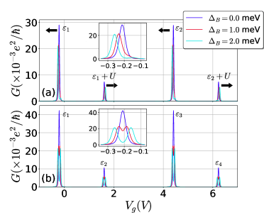
Fig.  4: (a) Conductance $G$ at $T=4$ K as a function of the gate voltage $V_{g}$ for different values of the Zeeman splitting $\Delta_{B}$ in the interacting model. We take two molecular levels with spacing $\Delta=140$ meV  ⁴, each split due to Coulomb repulsion. The couplings for the second level $\varepsilon_{2}$ are taken the same as for $\varepsilon_{1}$. Black arrows show how the peaks shift with increasing $\Delta_{B}$. (b) Same as (a) but in the noninteracting model with four single-particle resonances, which spin split as $\Delta_{B}$ enhances. The couplings for the third (fourth) level $\varepsilon_{3}$ ($\varepsilon_{4}$) are taken the same as for $\varepsilon_{1}$ ($\varepsilon_{2}$). Insets: leftmost conductance peaks from the main panels are zoomed in for better visualization.

The differing response to the presence of magnetic fields leads to distinct conductance curves for the interacting and the noninteracting cases. In the interacting theory, the level $\varepsilon_{m}$ in Eq. (12) becomes spin dependent, $\varepsilon_{m\sigma}=\varepsilon_{m}+s\Delta_{B}$ with $s=+$ ($-$) for $\sigma=\uparrow$ ($\downarrow$). In the noninteracting approach, both molecular levels in Eq. (14) become spin dependent as $\varepsilon_{i}\rightarrow\varepsilon_{i\sigma}$. The peak amplitude depends on $T$ and the particular choice of $\gamma$ and is thus sample-dependent (e.g., in the Electronic Supplementary Information^† we show that a different choice of $\gamma$ causes the lower resonance to have a smaller amplitude compared to the Coulomb-shifted one, in contrast to Fig. 4).

The effects of the magnetic field in both models are shown in Fig. 4. We depict the electric conductance $G=(dI/dV)|_{V=0}$ as a function of the gate voltage for different values of the Zeeman strength $\Delta_{B}$. For interacting particles [Fig. 4(a) for two energy levels $\varepsilon_{1}$ and $\varepsilon_{2}$ with interaction] the $G$ peak separation expands or shrinks as $\Delta_{B}$ increases, as anticipated above. This is a clear manifestation of a Coulomb-blockade split resonance. Contrary to this case, the interacting model [Fig. 4(b) for four energy levels $\varepsilon_{1}$, $\varepsilon_{2}$, $\varepsilon_{3}$ and $\varepsilon_{4}$ without interaction] leads to peak splittings when $B$ is such that $\Delta_{B}\simeq\Gamma$.

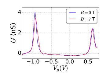
Fig.  5: Experimental differential conductance measurement of a ferrocene-based single molecular tunnel junction for two values of the magnetic field $B$ at a voltage bias of $|V_{sd}|=80$ mV. Clearly, both conductance peaks are shifted as $B$ increases, which suggests that charging effects are the main transport mechanism.

To test our theoretical predictions, a room temperature electromigration-breaking three-terminal single-electron transistor with Au bias-drain electrodes and Al/Al₂O₃ back gates was used to study an individual S-(CH₂)₄-ferrocenyl-(CH₂)₄-S molecule [Fig. 1(c)] at low temperature (see Ref. ⁴ for details on device fabrication). Note that the molecules investigated in Ref. ⁴ were not tested with a magnetic field since its effect would not be observable at the lowest temperature (80 K) employed in that study. Figure 5 shows the differential conductance as a function of gate voltage through the ferrocene-based single molecule junction obtained in the absence of magnetic field (blue data) and with a 7-Tesla field applied (red data). The measurements were obtained at $T=4$ K with a bias voltage of 80 mV. Two peaks are clearly visible at $V_{g}=-1.95$ V and $0.65$ V. Upon application of a magnetic field, the peaks shift in voltage approaching each other (see the stability plot in the Electronic Supplementary Information^†). One possible scenario is that the magnetic field drags the ferrocene unit slightly, hence distorting the molecule and changing its coupling to the electrodes and gate. However, it is unlikely that this effect leads to such a large change in potential energy since it would change the transport excitation slopes, which is not observed in our data. Additionally, strain-induced changes in the electrostatic coupling of the molecule will not discriminate levels according to its spin value. We next argue that the most natural explanation is in terms of charging effects.

We first notice that the peaks in Fig. 5 do not Zeeman split under the action of the magnetic field, as it would be expected from two distinct charge degeneracy points arising from two different molecular levels. Instead, the peaks shift, conferring them a Coulomb blockade nature resulting from strong charging energy effects (as explained above). The gate voltage shifts are actually pretty similar for both peaks. For the left peak in Fig. 5 is $+18$ mV, while for the right peak is $-19$ mV. Indeed, using the coupling capacitances of the molecule with the respective electrodes, extracted from measurements at different bias voltages, the observed shift in gate voltage for each peak gives $\Delta_{S}=-1/2$ for the left peak in Fig. 5 and $\Delta_{S}=+1/2$ for the right peak (i.e. a net spin change of $\frac{1}{2}$ as it corresponds to adding an electron into the molecule). However, the peaks do not repel from each other in increasing magnetic field, as would be expected if originated from the same Coulomb-blockade energy level splitting. This means that the two observed peaks belong to two different Coulomb-blockaded energy levels, whose corresponding pairs lie beyond the measuring gate voltage window in this measurement. It is very likely that the associated charge states from left to right in Fig. 5 correspond to Fe³⁺, Fe²⁺ and Fe⁺¹. (Note that the Fe⁺¹ state can be observed at low temperatures similarly to the work of de Leon et al. in Ref. ⁴¹.) In any case, the observation of the gate voltage shift under the action of a magnetic field allows the unequivocal association of the differential conductance peaks to charging effects, and showcases a magnetic field as a powerful tool to determine the nature of transport excitations in single-molecule junctions.

7 Conclusions

In conclusion, we have shown that the temperature-dependent transport properties of molecular tunnel junctions can be explained using a fully interacting model that takes into account Coulomb blockade effects. Since a noninteracting theory with two molecular levels also agrees with the experimental data, it is natural to ask what the nature of a real resonance is. We have suggested that an externally applied magnetic field can be used as a transport spectroscopy tool that distinguishes between the two models. Employing values extracted from the experiment, we find that the conductance peaks of a molecular bridge with Coulomb interactions shift as the magnetic field increases while in the noninteracting case the transmission resonances are all Zeeman split. Finally, we report on conductance measurements in the presence of a magnetic field that point to Coulomb-blockaded resonances in a ferrocene-based molecular tunnel junction. Since charging energies are expected to be similar in molecular tunnel junctions, the interaction model is likely to apply in most transport experiments where molecules are in the weak coupling regime. In our case, the ferrocenyl units are weakly coupled to the electrodes due to the insulating character of the alkyl chains. Our work thus represents an important contribution that will help identify the transport regime of molecular junction experiments.

References

- 1 H. Park, J. Park, A. K. L. Lim, E. H. Anderson, A. P. Alivisatos and P. L. McEuen, Nature, 2000, 407, 57.
- 2 J. Park, A. N. Pasupathy, J. I. Goldsmith, C. Chang, Y. Yaish, J. R. Petta, M. Rinkoski, J. P. Sethna, H. D. Abruña, P. L. McEuen and D. C. Ralph Nature, 2002 417, 722.
- 3 L. H. Yu, Z. K. Keane, J. W. Ciszek, L. Cheng, M. P. Stewart, J. M. Tour, and D. Natelso, Phys. Rev. Lett., 2004, 93, 266802.
- 4 A. R. Garrigues, L. Wang, E. del Barco and C. A. Nijhuis, Nat. Commun., 2016, 7, 11595.
- 5 L. Venkataraman, J. E. Klare, C. Nuckolls, M. S. Hybertsen, and M. L. Steigerwald, Nature, 2006, 442, 904.
- 6 I. Díez-Pérez, J. Hihath, Y. Lee, L. Yu, L. Adamska, M. A. Kozhushner, I. I. Oleynik and N. Tao, Nat Chem., 2009, 1, 635.
- 7 R. C. Chiechi, E. A. Weiss, M. D. Dickey and G. M. Whitesides, Angew. Chem. Int. Ed., 2008, 47, 142.
- 8 W. F. Reus, M. N. Thuo, N. D. Shapiro, C. A. Nijhuis, and G. M. Whitesides, ACS Nano, 2012, 6, 4806.
- 9 C. A. Nijhuis, W. F. Reus, J. Barber, and G. M. Whitesides, J. Phys. Chem., 2012, 116, 14139.
- 10 D. Fracasso, H. Valkenier, J. C. Hummelen, G. Solomon, and R. C. Chiechi, J. Am. Chem. Soc., 2011, 133, 9556.
- 11 X. Chen, M. Roemer, L. Yuan, W. Du, D. Thompson, E. del Barco and C. A. Nijhuis, Nat. Nanotechnol., 2017, 110, 1.
- 12 D. Fracasso, M. I. Muglali, M. Rohwerder, A. Terfort, and R. C. Chiechi, J. Phys. Chem., 2013, 117, 11367.
- 13 R. L. McCreery, and A. Bergren, J. Adv. Mater., 2009, 21, 4303.
- 14 A. E. Haj-Yahia, O. Yaffe, T. Bendikov, H. Cohen, Y. Feldman, A. Vilan and D. Cahen, Adv. Mater., 2013, 25, 702.
- 15 C. M. Bowers, K. Liao, T. Zaba, D. Rappoport†, M. Baghbanzadeh, B. Breiten, A. Krzykawska, P. Cyganik, and G. M. Whitesides, Nano Lett., 2015, 9, 1471.
- 16 Y. Zhang, Z. Zhao, D. Fracasso and R. C. Chiechi, Isr. J. Chem., 2014, 54, 513.
- 17 J. C. Cuevas and E. Scheer, Molecular Electronics: An introduction to theory and experiment, (World Scientific Series in Nanoscience and Nanotechology, Vol. 1, 2010)
- 18 L. Yuan, R. Breuer, L. Jiang, M. Schmittel, and C. A. Nijhuis, Nano Lett., 2015, 15, 5506.
- 19 L. Yuan, N. Nerngchamnong, L. Cao, H. Hamoudi, E. del Barco, M. Roemer, R. K. Sriramula, D. Thompson and C. A. Nijhuis, Nat. Commun., 2015, 6, 6324.
- 20 H. J. Yoon, K. Liao, M. R. Lockett, S. W. Kwok, M. Baghbanzadeh, and G. M. Whitesides, J. Am. Chem. Soc., 2014, 136, 17155.
- 21 S. H. Choi, B. Kim, and C. D. Frisbie, Science, 2008, 320, 1482.
- 22 H. Yan, A. J. Bergren, R. McCreery, M. L. D. Roccac, P. Martind, P. Lafarge, and J. C. Lacroix, Proc. Natl Acad. Sci. USA, 2013, 110, 5326.
- 23 C. E. Smith, S. O. Odoh, S. Ghosh, L. Gagliardi, C. J. Cramer, and C. D. Frisbie, J. Am. Chem. Soc., 2015, 137, 15732.
- 24 L. Lafferentz, F. Ample, H. Yu, S. Hecht, C. Joachim, and L. Grill, Science, 2009, 323, 1193.
- 25 M. Koch, F. Ample, C. Joachim, and L. Grill, Nat. Nanotechnol., 2012 7, 713.
- 26 G. I. Livshits, A. Stern, D. Rotem,N. Borovok, G. Eidelshtein, A. Migliore, E. Penzo, S. J. Wind, R. D. Felice, S. S. Skourtis, J. C. Cuevas, L. Gurevich, A. B. Kotlyar and D. Porath, Nat. Nanotechnol., 2014, 9, 1040.
- 27 W. Li, L. Sepunaru, N. Amdursky, S. R. Cohen, I. Pecht, M. Sheves, and D. Cahen, ACS Nano, 2012, 6, 10816.
- 28 L. Sepunaru, I. Pecht, M. Sheves, and D. Cahen, J. Am. Chem. Soc., 2011, 133, 2421.
- 29 K. S. Kumar, R. R. Pasula, S. Lim, and C. A. Nijhuis, Adv. Mater., 2016, 28, 1824.
- 30 J. M. Thijssen and H. S. J. Van der Zant, Phys. Stat. Sol. (b), 2008, 245, 1455.
- 31 K. Lee, G. Kulkarni and Z. Zhong, Nanoscale, 2016, 8, 7755.
- 32 H. Lehmann, S. Willing, S. Möller, M. Volkmann and C. Klinke, Nanoscale, 2016, 8, 14384.
- 33 V. V. Shorokhov, D. E. Presnov, S. V. Amitonov, Y. A. Pashkin and V. A. Krupenin, Nanoscale, 2017, 9, 613.
- 34 L. P. Kouwenhoven, C. M. Marcus, P. L. McEuen, S. Tarucha, R. M. Westervelt, N. S. Wingreen, in Mesoscopic Electron Transport, ed. by L. L. Sohn, L. P. Kouwenhoven and G. Schön (Kluwer, Dordrecht, 1996).
- 35 K. Moth-Poulson and T. Bjornholm, Nat. Nanotechnol., 2009, 4, 551.
- 36 G. Heimel, S. Duhm, I. Salzmann, A. Gerlach, A. Strozecka, J. Niederhausen, C. Bürker, T. Hosokai, I. Fernandez-Torrente, G. Schulze, S. Winkler, A. Wilke, R. Schlesinger, J. Frisch, B. Bröker, A. Vollmer, B. Detlefs, J. Pflaum, S. Kera, K. J. Franke, N. Ueno, J. I. Pascual, F. Schreiber and N. Koch, Nat. Chem., 2013, 5, 187.
- 37 M. L. Perrin, C. J. O. Verzijl, C. A. Martin, A. J. Shaikh, R. Eelkema, J. H. van Esch, J. M. van Ruitenbeek, J. M. Thijssen, H. S. J. van der Zant and D. Dulić, Nat. Nanotechnol., 2013, 8, 282.
- 38 H. Haug and A. P. Jauho, Quantum Kinetics in Transport and Optics of Semiconductors (Springer, Berlin, 2008)
- 39 Y. Meir, N. S. Wingreen, and P. A. Lee, Phys. Rev. Lett., 1991, 66, 3048.
- 40 M. Poot, E. Osorio, K. O’Neill, J. M. Thijssen, D. Vanmaekelbergh, C. A. van Walree, L. W. Jenneskens, and H. S. J. van der Zant, Nano Lett., 2006, 6, 1031.
- 41 N. P. de Leon, W. Liang, Q. Gu, and H. Park, Nano Lett., 2008, 8, 2963.
- 42 Z. Xie, I. Baldea, C. E. Smith, Y. Wu, and C. D. Frisbie, ACS Nano, 2015, 9, 8022.
- 43 E. Burzuri and H. S. J. van der Zant, Single-molecule spintronics, in Molecular Magnets. Physics and Applications (Springer, Berlin, 2014), pp. 297–318.
- 44 D. S. Duncan, D. Goldhaber-Gordon, R. M. Westervelt, K. D. Maranowski and A. C. Gossard, Appl. Phys. Lett., 2000, 77, 2183.