A Comprehensive Study of $g$-Factors, Elastic, Structural and Electronic Properties of III-V Semiconductors using Hybrid-Density Functional Theory

Abstract

Despite the large number of theoretical III-V semiconductor studies reported every year, our atomistic understanding is still limited. The limitations of the theoretical approaches to yield accurate structural and electronic properties on an equal footing, due to the unphysical self-interaction problem that affects mainly the band gap and spin-orbit splitting (SOC) in semiconductors and, in particular, III-V systems with similar magnitude of the band gap and SOC. In this work, we will report a consistent study of the structural and electronic properties of the III-V semiconductors employing the screening hybrid-DFT framework, fitting the $\alpha$ parameters for $12$ different III-V compounds, namely, AlN, AlP, AlAs, AlSb, GaN, GaP, GaAs, GaSb, InN, InP, InAs, InSb, in order to minimize the deviation between the theoretical and experimental values of the band gap and SOC. Structural relaxation effects were also included. Except for AlP, whose $\alpha=$0.127$$, we obtained $\alpha$ values spreading from $0.209$ to $0.343$, deviating less than $0.1$ from the universal value of $0.25$. Our results for the lattice parameter and elastic constants indicate that the fitting of the $\alpha$ does not affect those structural parameters when compared with the HSE06 functional, where $\alpha=$0.25$$. Our analysis of the band structure based on the $\textbf{k}{\cdot}\textbf{p}$ method shows that the effective masses are in agreement with the experimental values, which can be attributed to the simultaneous fitting of the band gap and SOC. Finally, we estimate the values of $g$-factors, extracted directly from band structure, which are close to experimental results indicating that the obtained band structure produced a realistic set of $\textbf{k}{\cdot}\textbf{p}$ parameters.

I Introduction

Semiconductors have been playing a key role in the development of new technologies since the 50’s, e.g., light-emitting diodes and lasers,Schubert (2006); Nakamura (2015); Sun et al. (2016) infrared detectors,Rogalski (2010) solar cells Nelson (2003) and more recently, spin-lasers,Basu et al. (2008) and etc. Those developments have been possible due to the large number of fundamental studies employing theoretical or experimental techniques along decades.Yu and Cardona (1999); Enderlein (1997) which have contributed to the present understanding of the semiconductors electronic band-structure properties, punctual and extended defects, and structural control.Enderlein (1997); Madelung (2004) Beyond that, new fields have emerged along the years such as topological insulatorsHasan and Kane (2010) and Majorana fermions in nanowires,Stanescu et al. (2011); Mourik et al. (2012) which are expected to contribute to future technological applications.

Among a wide range of semiconductor materials,Enderlein (1997); Madelung (2004); Yu and Cardona (1999); Bushby et al. (2013) the III-V AB semiconductors, where A = Al, Ga, In and B = N, P, As, Sb (i.e., $12$ compounds), occupy an important place due to their role in several technological developments.Nelson (2003); Schubert (2006); Basu et al. (2008); Rogalski (2010); Nakamura (2015) Although there is an impressive number of papers published every year based on experimental and/or first-principles calculations,Gmitra and Fabian (2016); Sandoval et al. (2016); Polly et al. (2016); Seghilani et al. (2016); Faria Junior et al. (2016); Zhao et al. (2016); Nestoklon et al. (2016); Sun et al. (2016) our atomistic understanding is still limited, in particular, due to the limitations in theoretical approaches to describe structural and electronic properties on an equal footing. For example, first-principles calculations based on density functional theory (DFT) with local or semilocal exchange-correlation energy functionals suffer from the unphysical self-interaction problem,Perdew and Zunger (1981); Perdew and Levy (1983); Jones and Gunnarsson (1989) which affects mainly the band gap and spin-orbit splitting (SOC) in semiconductorsPerdew and Levy (1983); Kim et al. (2010) and, in particular for few III-V AB semiconductors, where the SOC can have similar magnitude as the band gap, e.g., GaSb, InP, InAs and InSb.Adachi (1992); Madelung (2004)

Along the years, the self-interaction problem has motivated the widespread use of approximations or alternative descriptions of the electronic states such as the GW Hedin (1965); Aryasetiawan and Gunnarsson (1998) or nonlocal hybrid density-functionals, e.g., PBE0,Perdew et al. (1996a); Adamo and Barone (1999) HSE06,Heyd et al. (2003); Heyd and Scuseria (2004); Heyd et al. (2006) and B3LYP,Becke (1993) and etc. In principle, both GW and hybrid-DFT can yield an improved description of the band structure compared with local or semilocal functionals, however, GW was designed to address electronic properties but not the structural properties.Hedin (1965); Aryasetiawan and Gunnarsson (1998) In contrast with GW, hybrid-DFT can describe both structural and electronic properties on an equal footing, however, the electronic properties such as the band gap depends strongly on the magnitude of the nonlocal Fock exchange, $\alpha$, that replaces part of the semilocal exchange term. Although an universal value for $\alpha$ was suggested, i.e., $25\text{\,}\mathrm{\char 37\relax}$ in PBE0,Perdew et al. (1996a); Heyd et al. (2003) it is not as universal as expected.Viñes et al. (2017)

As the band increases almost linearly by increasing the magnitude of the nonlocal Fock exchange,Moses et al. (2011) several studies have proposed a fitting of the $\alpha$ parameter to improve the description of the band gap.Viñes et al. (2017); Bastos et al. (2016); Moses et al. (2011) However, those studies have employed, in most cases, atomic structures optimized with the local or semilocal functionals,Ramos et al. (2001); Dal Corso (2012); Paier et al. (2006) i.e., the differences in the structural parameters are neglected. This is a good approximation but it might fail in cases in which the fine details of the electronic structure depend strongly on the lattice parameters, e.g., III-V systems with large SOC.

In this work, we propose to perform a consistent study of the structural and electronic properties of the III-V semiconductors employing the screening hybrid-DFT framework, where the $\alpha$ parameters for the different compounds are fitted by the minimization of the deviation between the theoretical and experimental values for the band gap and SOC. We also employed optimized lattice parameters based on screening hybrid-DFT, i.e., small differences in the lattice constant were taken into account for the electronic parameters. Based on this framework, we calculated the equilibrium lattice constant, elastic constants, bulk modulus, band structures, effective masses, and etc. Furthermore, we employed the $\mathbf{k{\cdot}p}$ method to perform a deep analysis of the band structures, from which were possible to extract the $\mathbf{k{\cdot}p}$ parameters and the electronic $g$-factors.

Except for AlP, we obtained $\alpha$ parameters spreading from $0.209$ to $0.343$, i.e., close to the universal value of $0.25$. For AlP, the calculated $\alpha$ value is $0.127$. Based on several analyses, we found with small exceptions, that the $\alpha$ values correlate well with the atomic radius of the cationic species and hence, further $\alpha$ values for different semiconductors could be extrapolated from this finding without additional calculations. Our results for the lattice and elastic constants indicate that the fitting of the $\alpha$ does not affect those structural parameters when compared with the HSE06 functional, where $\alpha=0.25$.

Our analysis of the band structure based on the $\mathbf{k{\cdot}p}$ method shows that the effective masses are in agreement with the experimental values,Madelung (2004); Vurgaftman et al. (2001) i.e, the fitting of $\alpha$ at the $\Gamma$ point improved the description of the band curvatures. We also determined the $g$-factors directly from the effective band structures finding values that are close to the experimental results.Adachi (1992); Madelung (2004) Finally, having both, $g$-factors and effective masses, in good agreement with the experimental results indicates that we have determined realistic sets of $\mathbf{k{\cdot}p}$ parameters.

II Theoretical Approach and Computational Details

II.1 Density Functional Theory

It has been known for decades that DFT Hohenberg and Kohn (1964); Kohn and Sham (1965) within local (local density approximation – LDA) Perdew and Wang (1992) or semilocal (generalized gradient approximation – GGA) Perdew et al. (1992, 1996b) exchange-correlation energy functionals is unable to yield a correct description of the fundamental band gap even for the most simple systems,Perdew and Levy (1983); Kim et al. (2010) which has been attributed mainly to the unphysical self-interaction problem.Perdew and Zunger (1981); Perdew and Levy (1983); Jones and Gunnarsson (1989) This limitation has motivated the widespread use of approximations or alternative descriptions of the electronic valence states such as the GW Hedin (1965); Aryasetiawan and Gunnarsson (1998) or nonlocal hybrid functional, e.g., PBE0,Ernzerhof and Scuseria (1999); Adamo and Barone (1999) HSE06,Heyd et al. (2003); Heyd and Scuseria (2004); Heyd et al. (2006) and B3LYP.Becke (1993) In principle, both GW and nonlocal hybrid functionals can yield an improved description of the band structure compared with LDA or GGA. However, in contrast with the GW framework, nonlocal hybrid functional can provide also a reliable description of the structural and energetics properties,Paier et al. (2006); Da Silva et al. (2007); Ganduglia-Pirovano et al. (2009); Hinuma et al. (2014) which is a plus compared with GW.

In this work, we will employ the DFT framework within the GGA formulation proposed by Perdew–Burk–ErnzerhofPerdew et al. (1996b) (PBE) and the hybrid functional proposed by Heyd–Scuzeria–ErnzerhofHeyd et al. (2003); Heyd and Scuseria (2004); Heyd et al. (2006) (HSE) in which the magnitude of the nonlocal Fock exchange replaces part of the PBE exchange. As will be described bellow, we will fit the magnitude of the nonlocal Fock exchange based on the experimental results of the fundamental band gap and the spin-orbit splitting, while using the same screening parameter derived for the HSE06 functional.Krukau et al. (2006); Heyd et al. (2006)

To describe the electronic states, we employed the scalar-relativistic approximationKoelling and Harmon (1977); Takeda (1978) in which relativistic corrections are considered for the core-states, while the SOC is not considered for the valence states, and hence, the spin-orbit splitting for the III-V semiconductors cannot be described. For example, for InSb the SOC splitting at the $\Gamma$-point and valence band maximum (VBM), has similar magnitude as the fundamental band gap,Madelung et al. (1982); Kim et al. (2010) and hence, it plays a crucial role for the characterization of the band structure parameters, e.g., effective mass, $g$-factor, etc. Thus, to improve the description of the band structure properties, we employed the addition of the SOC for the valence states via the second-variational approach.Koelling and Harmon (1977)

To solve the Kohn–Sham equations, we employed the projected augmented wave (PAW) method,Blöchl (1994) as implemented in the Vienna ab initio simulation package (VASP, version $5.4.1$),Kresse and Hafner (1993); Kresse and Furthmüller (1996) employing the PAW projectors provided with the package.Kresse and Joubert (1999) To describe the electronic states, the Kohn–Sham orbitals are expanded in plane waves employing a finite cutoff energy, which depends on the calculated properties. This is necessary since several properties, e.g., stress tensor and elastic constants converge slowly as the number of plane waves increases.

From a large number of PBE and HSE convergence tests, we demonstrated that well converged total energies, band structures, and densities of states can be obtained by using a cutoff energy that is $1.125$ times the recommended maximum cutoff energy (ENMAX${}_{\text{max}}$). Stress tensor and elastic constants calculations, however, require at least $1.50\times\text{ENMAX}_{\text{max}}$. A further increase in the cutoff energy can improve the results slightly, and for the particular case of the PBE calculations, we increased the multiplication factor from $1.50$ to $2.0$ (stress tensor) and to $2.5$ (elastic constants) aiming to provide reference data that can be used for further comparisons. For example, for AlN, we employed $473\text{\,}\mathrm{eV}$ for total energy and band structure; $631\text{\,}\mathrm{eV}$ (HSE) and $841\text{\,}\mathrm{eV}$ (PBE) for stress tensor; and $631\text{\,}\mathrm{eV}$ (HSE) and $1052\text{\,}\mathrm{eV}$ (PBE) for the elastic constants calculations. For the Brillouin zone integration, we employed a Monkhorst–Pack k-mesh of $10{\times}10{\times}10$, while the same k-point density was employed for the remaining III-V semiconductors. All those parameters are provided in the Supplementary Material.

To obtain the equilibrium volume, we minimized the stress tensor, which was performed by several consecutive optimizations of the equilibrium volume to ensure that the optimized equilibrium volume is consistent with the initial set up of the basis size. To calculate the elastic properties, we considered the combination of two schemes, namely, $(i)$ rigid lattice parameters obtained from the stress-tensor optimization,Page and Saxe (2002) and $(ii)$ ionic volume relaxation from the inversion of the ionic Hessian matrix and internal stress tensor,Wu et al. (2005) as implemented in VASP. For those calculations, we employed atomic steps of $0.010\text{\,}\mathrm{\SIUnitSymbolAngstrom}$, which are slightly smaller than the recommended value by VASP, e.g., $0.15\text{\,}\mathrm{\SIUnitSymbolAngstrom}$.

II.2 Hybrid HSE Functional: Fitting of the $\alpha$ Value

The hybrid PBE0 functional is composed by the PBE correlation energy and a fraction of $25\text{\,}\mathrm{\char 37\relax}$ of the PBE exchange is replaced by the nonlocal Fock exchange of the Hartree–Fock (HF) method, i.e., $E_{\text{XC}}^{\text{PBE0}}=E_{\text{c}}^{\text{PBE}}+{\alpha}E_{\text{x}}^{\text{HF}}+(1-{\alpha})E_{\text{x}}^{\text{PBE}}$, where $\alpha=$0.25$$.Ernzerhof and Scuseria (1999); Adamo and Barone (1999) The hybrid HSE functionalHeyd et al. (2003); Heyd and Scuseria (2004); Heyd et al. (2006) is derived from PBE0 by using a screening function to split the semilocal PBE exchange and nonlocal Fock term into two parts, namely, a short- (SR) and long-range (LR) exchange contributions, in which the nonlocal Fock LR contribution cancel with part of the PBE LR exchange. Thus, the hybrid HSE functional is given by the following equation,

$$\begin{split}E_{\text{XC}}^{\text{HSE}}=&E_{\text{c}}^{\text{PBE}}+E_{\text{x}}^{\text{PBE,LR}}(\omega)+\alpha E_{\text{x}}^{\text{HF, SR}}(\omega)\\ &+(1-\alpha)E_{\text{x}}^{\text{PBE,SR}}(\omega)~{},\end{split}$$ (1)

where the new parameter, $\omega$, measures the intensity of the screening, and hence, the extension of the nonlocal Fock interactions. For example, if $\omega$ is null, the SR contribution is equivalent to the full Fock operator and the LR contribution will become zero, while for ${\omega}{\rightarrow}{\infty}$, the range of SR terms decrease, recovering asymptotically the PBE functional. As defined in the PBE0 functional, the parameter $\alpha$ controls the amount of PBE exchange replaced by the nonlocal Fock exchange, and hence, in principle, it can ranges from $0$ to $1$. For the hybrid HSE06 functional, $\alpha=0.25$ and $\omega=$0.206\text{\,}\mathrm{\SIUnitSymbolAngstrom}^{-1}$$, which were obtained from the adiabatic perturbation theory and fitted from a large number of systems, respectively.Heyd et al. (2006); Krukau et al. (2006)

Although, the hybrid HSE06 functional yield better results than the LDA and GGA functionals, HSE06 does not yield the experimental band gaps in most of the cases,Heyd et al. (2005); Kim et al. (2009, 2010) and hence, improved results can be obtained by fitting the $\omega$ or $\alpha$ parameters. Recently, Viñes et al. Viñes et al. (2017) suggested that a large number of combination of $\omega$ and $\alpha$ values can yield the band gap of oxides, however, it is important to mention that the fitting of $\omega$ can affect drastically the small contribution of the LR nonlocal Fock terms, which has the potential to decrease the stability of the electron density convergence. In contrast with $\omega$, the fitting of $\alpha$ affects mainly the SR nonlocal Fock contribution, which plays a crucial role in the physical properties.Perdew et al. (2017); Atalla et al. (2016); Sai et al. (2011); Yang et al. (2012)

Therefore, to improve the description of the experimental fundamental band gap, $E_{\text{gap}}$, and the spin-orbit (SO) splitting energies, ${\Delta}_{\text{so}}$, we fixed the $\omega$ parameter to the same value used in HSE06, and fitted the $\alpha$ parameter to reproduce the experimental $E_{\text{gap}}$ and ${\Delta}_{\text{so}}$ results. The fitting was performed using the linear dependence of $E_{\text{gap}}$ and $\Delta_{\text{so}}$ as a function of $\alpha$, which is well known in the literature.Walsh et al. (2008); Komsa and Pasquarello (2011); Colleoni and Pasquarello (2016) Due to the nearly perfect linear dependence, the angular coefficient (slope), can be calculated using two points, namely, using the $E_{\text{gap}}$ or $E_{\Delta_{\text{so}}}$ values calculated with the PBE $(\alpha=0)$ and HSE06 $(\alpha=0.25)$ functionals. Thus, the angular coefficient for the fitting of the band gap is given by the following relation,

$$m_{\text{gap}}=\frac{E_{\text{gap}}^{\text{HSE06}}-E_{\text{gap}}^{\text{PBE}}}{0.25}~{},$$ (2)

while $m_{\Delta_{\text{so}}}$ is obtained by replacing the band gap energies by the spin-orbit splittings. Thus, the $\alpha$ value that yields the experimental band gap, $E^{\text{exp}}_{\text{gap}}$, or the experimental spin-orbit splitting, $E^{\text{exp}}_{\Delta_{\text{so}}}$, can be obtained from the following equation,

$$\alpha_{\text{gap}}=\frac{E^{\text{exp}}_{\text{gap}}-E_{\text{gap}}^{\text{PBE}}}{m_{\text{gap}}}~{}.$$ (3)

Consequently, from this scheme, we obtained two values for $\alpha$, namely, an optimized value for $\alpha_{\text{gap}}$ ($\alpha_{\Delta_{\text{so}}}$) that yields the experimental band gap (spin-orbit splitting). To obtain an unique $\alpha$ for each III-V system, we performed a minimization of the standard deviation between the experimental and the extrapolated $E^{\text{exp}}_{\text{gap}}$ and $E^{\text{exp}}_{\Delta_{\text{so}}}$ parameters obtained from the slope. Further technical details are reported in the Supplementary Material. Thus, from now on, the fitted hybrid HSE functional will be noted HSE_α, where $\alpha$ is different for each semiconductor. Finally, in order to compare our results with literature and among different functionals, we adopted, as a measure, the normalized-root-mean-square deviation (NRMSD).Todeschini et al. (2009)

III Results

III.1 Magnitude of the Non-Local Fock Exchange

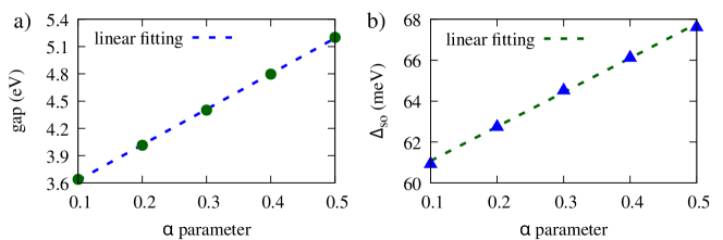
Figure 1: Linear dependence of the band gap (right) and $\Delta_{\text{so}}$ (left) on the $\alpha$ parameter for AlP.

Except for AlP, the optimal $\alpha$ values that minimize the relative errors for the undamental band gap and SOC splitting are in between $0.209$ and $0.343$, i.e., close to the universal value of $0.25$.Perdew et al. (1996a) For AlP, the value if $0.127$. Therefore, we can conclude that an unique $\alpha$ value is unable to yield the fundamental band gap and SOC splitting for a wide range of compounds, as well as further physical properties, which have also been reported in the few previous studies.Walsh et al. (2008) Although the value of $\alpha$ has been obtained from a solid theoretical framework, few studies have tried to obtain a correlation between the magnitude of $\alpha$ and a particular physical property,Viñes et al. (2017) which can help in several applications. Thus, with the aim to identify the most important physical parameters that play the major role in the magnitude of $\alpha$, we performed several analyses (also in the Supplementary Material). Among all analyses, we found a good correlation between the magnitude of $\alpha$ versus the cationic radius,Slater (1964) which is shown in Fig. 1. Our results indicate that the value of the optimized $\alpha$ decreases almost linearly as a function of the atomic cationic radius, except for the cases of AlN and AlP.

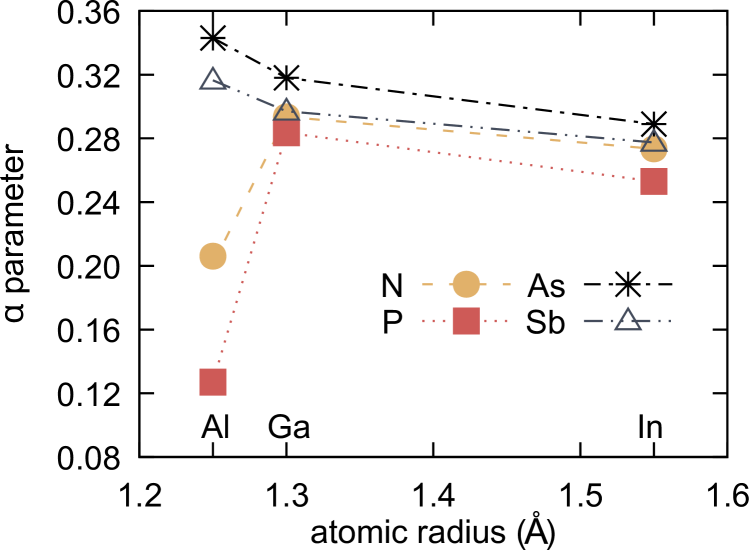
Figure 1: Optimal magnitude of the nonlocal Fock exchange, $\alpha$, in the hybrid HSE_α functional obtained from the fitting of the fundamental band gap and the spin-orbit coupling versus the cation atomic radii obtained from Ref. Slater, 1964. The atomic radii are given in $\mathrm{\SIUnitSymbolAngstrom}$ and $\alpha$ is dimensionless.

III.2 Equilibrium Lattice Parameter

The most stable crystalline phase of the III-V semiconductors is the zinc-blende structure,Kittel (2004) which has a face-centered cubic (fcc) lattice and $\text{F}\bar{4}3\text{m}$ space group. The exception for this rule are the III-nitrides (AlN, GaN, InN) that prefer to crystallize in the hexagonal wurtzite structure, belonging to the $\text{P}6_{3}\text{mc}$ space group,Morkoç (2009) but through the use of experimental techniques such as molecular beam epitaxy can also be grown as a zinc-blende structure.Yu and Cardona (1999); Morkoç (2009) Thus, to rationalize our understanding, all the III-V semiconductors were studied in the zinc-blende structure, which contains two fourfold atoms with tetrahedral local symmetry. The equilibrium lattice parameter, $a_{0}$, was calculated using several approximations, namely, PBE, PBE+SOC, HSE06, and HSE_α, and the results are summarized in Table 1 along with the experimental results.

Table 1: Equilibrium lattice parameters $a_{0}$ (in $\mathrm{\SIUnitSymbolAngstrom}$) for all the III-V semiconductors, calculated with the PBE, PBE with spin-orbit coupling for the valence states (PBE+SOC), HSE06, and HSE_α functionals. For the hybrid HSE_α functional, the adjusted $\alpha$ parameter is indicated within parentheses. The NRMSD indicates the normalized percentage deviation between theoretical and experimental parameters for the full series.

	PBE	PBE+SOC	HSE06	HSEα ($\alpha$)	Exp.
AlN	$4.399$	$4.399$	$4.361$	$4.367$ ($0.219$)	$4.38$a
AlP	$5.505$	$5.505$	$5.471$	$5.487$ ($0.127$)	$5.46$b
AlAs	$5.731$	$5.731$	$5.678$	$5.660$ ($0.343$)	$5.661$b
AlSb	$6.213$	$6.215$	$6.160$	$6.146$ ($0.318$)	$6.135$b
GaN	$4.545$	$4.545$	$4.492$	$4.483$ ($0.293$)	$4.52$a
GaP	$5.499$	$5.499$	$5.456$	$5.449$ ($0.283$)	$5.45$b
GaAs	$5.742$	$5.738$	$5.669$	$5.652$ ($0.318$)	$5.653$b
GaSb	$6.203$	$6.203$	$6.124$	$6.124$ ($0.297$)	$6.095$b
InN	$5.042$	$5.039$	$4.976$	$4.956$ ($0.274$)	$4.97$c
InP	$5.946$	$5.942$	$5.886$	$5.885$ ($0.253$)	$5.868$b
InAs	$6.174$	$6.172$	$6.090$	$6.078$ ($0.289$)	$6.058$b
InSb	$6.619$	$6.618$	$6.526$	$6.549$ ($0.277$)	$6.479$b
NRMSD	$1.49$	$1.47$	$0.40$	$0.49$	-

• from Ref. Pearton, 2000,

• from Ref. Madelung, 2004,

• from Ref. Rössler, 2011

In agreement with previous DFT-PBE calculations,Anua et al. (2013); Heyd et al. (2005); Dal Corso (2012) we obtained equilibrium PBE lattice constants that overestimate experimental results, with the largest deviation smaller than $2.2\text{\,}\mathrm{\char 37\relax}$ for InSb. The addition of the SOC for the valence states reduces the lattice constant only in the third decimal place, and hence, the improvement over the PBE compared with the experimental results is almost negligible and can be evaluated by the NRMSD show in Table 1. For example, the NRMSD is $1.49\text{\,}\mathrm{\char 37\relax}$ for PBE and $1.47\text{\,}\mathrm{\char 37\relax}$ for PBE+SOC. Therefore, the SOC does not affect the equilibrium lattice constants in contrast with the electronic properties, where it plays an essential role (see below).

In order to reduce the computational cost, which increases substantially for HSE06+SOC, the HSE06 and HSE_α equilibrium lattice constants were calculated using stress tensor without the addition of the SOC for the valence states. The HSE06 and HSE_α functionals yield $a_{0}$ parameters closer to the experimental results, and hence, with smaller relative errors compared with the PBE results. These small errors were expected since we provided an improved description of the exchange energy by the nonlocal Fock term. The differences between the HSE06 and HSE_α results are very small, i.e., the NRMSD changes from $0.4\text{\,}\mathrm{\char 37\relax}$ (HSE06) to $0.49\text{\,}\mathrm{\char 37\relax}$ (HSE_α), which is an important result since it shows that the lattice parameters were only slightly affected by the improvement of the description of the fundamental band gap and spin-orbit splitting at the $\Gamma$-point. The HSE06 results are in excellent agreement with previous hybrid HSE06 results,Kim et al. (2009) e.g., indium composites have differences smaller than $0.3\text{\,}\mathrm{\char 37\relax}$, $0.4\text{\,}\mathrm{\char 37\relax}$, $0.5\text{\,}\mathrm{\char 37\relax}$ for InP, InAs and InSb, respectively.

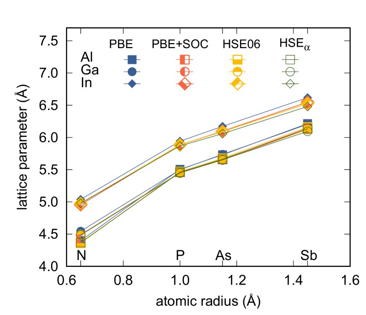
Figure 2: Lattice parameters versus the atomic radius of the anion species. The lattice parameters were obtained using the following exchange-correlation functionals: PBE, PBE+SOC, HSE06, HSE_α. The atomic radii were extracted from Ref. Slater, 1964.

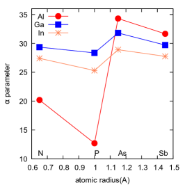
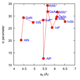
Figure 2: Cation atomic radius (left) and lattice parameter(right) dependence on the $\alpha$ parameter.

The lattice parameter have a slight linear dependence with the atomic radius of the material compound elements (occupation of the electronic shells), i.e., if the anionic atom size increases, the lattice parameter also increases, as showed in Fig. 2. This effect occurs due to the electrostatic repulsion between atoms, i.e., the bond length depends on the atom size, changing the lattice parameter. As Al and Ga have similar atomic radii, with $1.25\text{\,}\mathrm{\SIUnitSymbolAngstrom}$ and $1.30\text{\,}\mathrm{\SIUnitSymbolAngstrom}$, respectively,Slater (1964) the lattice parameters for the Al-V compounds are closer to the Ga-V values, as showed in the figure. The In has a greater atomic radius, $1.55\text{\,}\mathrm{\SIUnitSymbolAngstrom}$,Slater (1964) resulting in a larger lattice parameter for the In-V compounds. In order to investigate the linearity break shown for the III-N compounds, we evaluated the effective Bader charge, as shown in the table 6 in appendix B. The III-N compounds have a large charge transfer, which suggests that the break in the linearity behavior is due to the high ionicity combined with the smaller atomic radius of the N when when compared with the other cations of the III-A column of the Periodic Table. This hypothesis is also supported by the fact that the III-N compounds showed the highest elastic constants values in the series, as will be discussed in the next section, and the larger observed bond strengths.Nak (2000)

III.3 Elastic constants

Table 2: Elastic constants calculated with PBE and $\alpha$-optimized HSE (HSE_α), functionals. The bulk moduli, $B_{0}$, were obtained from the elastic constants results, namely, $B_{0}=(C_{11}+2C_{12})/3$, and are compared with the experimental values obtained from elastic constants (Exp.${}^{C_{ij}}$) and direct measures (Exp.${}^{B_{0}}$). All constants are given in $\mathrm{GPa}$.

		$C_{11}$				$C_{12}$				$C_{44}$					$B_{0}$
	PBE	HSEα	Exp.		PBE	HSEα	Exp.		PBE	HSEα	Exp.		PBE	HSEα	Exp.${}^{C_{ij}}$	Exp.${}^{B_{0}}$
AlN	$283.1$	$308.1$	-		$149.8$	$161.6$	-		$179.2$	$197.2$	-		$194.2$	$210.5$	-	-
AlP	$125.8$	$133.6$	$141$a		$61.3$	$65.1$	$62$a		$60.8$	$64.1$	$70$a		$82.8$	$87.9$	$88.3$	-
AlAs	$103.9$	$122.1$	$122$a		$49.1$	$58.5$	$57$a		$51.1$	$59.0$	$60$a		$67.4$	$79.7$	$78.7$	74c
AlSb	$77.0$	$93.7$	$88$a		$35.8$	$43.2$	$40$a		$36.8$	$47.5$	$43$a		$49.5$	$60.0$	$56.0$	55.1 d
GaN	$253.3$	$290.0$	-		$125.2$	$149.0$	-		$146.4$	$173.9$	-		$167.9$	$196.0$	-	-
GaP	$124.6$	$150.0$	$140$a		$56.0$	$64.3$	$62$a		$65.2$	$78.4$	$70$a		$78.9$	$92.9$	$88.0$	-
GaAs	$98.1$	$122.0$	$119$a		$42.1$	$49.4$	$53$a		$50.8$	$65.3$	$60$a		$60.8$	$73.6$	$75.0$	-
GaSb	$74.6$	$90.1$	$88$a		$32.0$	$35.7$	$40$a		$35.9$	$49.0$	$43$a		$46.2$	$53.8$	$56.0$	-
InN	$159.3$	$188.7$	-		$102.0$	$125.8$	-		$78.9$	$93.3$	-		$121.1$	$146.8$	-	-
InP	$87.4$	$105.9$	$101$b		$45.9$	$56.4$	$56$b		$41.9$	$49.3$	$46$b		$59.7$	$72.9$	$71.0$	-
InAs	$70.9$	$91.5$	$83$a		$37.8$	$48.8$	$45$a		$33.1$	$42.4$	$40$a		$48.8$	$62.7$	$57.6$	58e
InSb	$55.3$	$74.1$	$69$a		$29.1$	$34.8$	$37$a		$25.4$	$39.0$	$31$a		$37.8$	$47.9$	$47.7$	-
NRMSD ( %)	$14.3$	$4.9$	-		$15.0$	$5.1$	-		$13.8$	$9.2$	-		$14.4$$\dagger$	$3.7$$\dagger$	-	-

• Ultrasound Ref. Martienssen and Warlimont, 2005,

• Ultrasonic-wave transit times Ref. Martienssen and Warlimont, 2005,

• X-ray diffraction data from Ref. Madelung, 2004,

• Energy dispersive X-ray from Ref. Madelung, 2004

• Ultrasound from Ref. Madelung, 2004

• Comparison with Exp.${}^{C_{ij}}$

The cubic zinc-blende crystal structure has the symmetry defined by the space group $\text{F}\bar{4}3\text{m}$ that is associated to the point group $T_{d}$.Yu and Cardona (1999) The symmetry analysis show that it possess only three non-equivalent elastic constants: $C_{11}$, $C_{12}$ and $C_{44}$. $C_{11}$ represents the modulus for the axial compression, i.e., the stress in one direction induces a strain in the same direction. In contrast, $C_{12}$ represents the stress that induces a strain in the perpendicular directions and $C_{44}$, the shear modulus, represents the strain across the faces induced by the stress in a direction parallel to it. PBE, HSE_α and the respective experimental results of $C_{11}$, $C_{12}$ and $C_{44}$ are shown in Table 2. We also present the bulk modulus, $B_{0}$, which were calculated from the expression $B_{0}=(C_{11}+2C_{12})/3$.

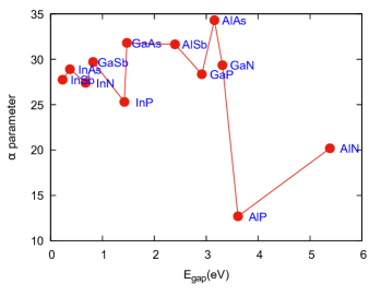
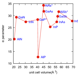
Figure 3: Energy gap (left) and equilibrium volume (right) dependence on the $\alpha$ parameter.

Unrelated to the exchange and correlation functionals, the elastic constants in all directions decrease as the ionic radius increase. For the PBE functional, e.g., $C_{11}$ decreases from $283.1$ in AlN to $77$ in AlSb. The ionic bond character is responsible for the increase on the hardness of the material, and as shown in the table 6 in appendix B, the ionicity (related with the Bader charge) decreases as the anion radius decreases. Therefore, it is expected that the elastic constant decreases as the lattice parameter (associated with the cation and anion radii) of the crystal structure increases. In fact, our results indicate a slight linear dependence with the lattice parameter, as showed in Fig. 3, where the dashed line shows a linear fitting using the all materials, nitrides excluded. This behavior was reported in the literatureAdachi (1992); Keyes (1962) and was traditionally used to estimate the elastic constantsWillardson and Beer (1975); Adachi (1985) by the extrapolation of the data.

In contrast with the lattice parameter overestimation by HSE functionals, the PBE functional underestimates the elastic constants in all the directions, which is consistent with the literature.Łopuszyński and Majewski (2007) On the other hand, the HSE_α results show better agreement with the experimental results, presenting NRMSDs of $4.9\text{\,}\mathrm{\char 37\relax}$ and $5.1\text{\,}\mathrm{\char 37\relax}$ for $C_{11}$ and $C_{12}$, respectively. The inclusion of nonlocal effects in the Fock exchange in HSE_α suggests an increasing of the bond hardness, consequently increasing the elastic constants when compared to the PBE functional. For $C_{44}$, our results when compared with the experimental data, show deviations for the HSE_α functional similar to the PBE ones, presenting NMRSDs of $13.8\text{\,}\mathrm{\char 37\relax}$ and $9.2\text{\,}\mathrm{\char 37\relax}$, respectively. Similar $C_{44}$ values have been found by Caro et al.Caro et al. (2012) using the HSE06 for nitrides. Nonetheless, PBE underestimates the experimental values of $C_{11}$ and $C_{12}$, while HSE_α overestimates them. Since the bulk modulus, $B_{0}$, in a cubic system has dependence only in the $C_{11}$ and $C_{12}$ elastic constant directions, the PBE functional also underestimates the $B_{0}$ values, while the HSE_α functional yields better results. This can be observed by the NRMSD which is $3.7\text{\,}\mathrm{\char 37\relax}$ and $14.4\text{\,}\mathrm{\char 37\relax}$ for HSE_α and PBE, respectively.

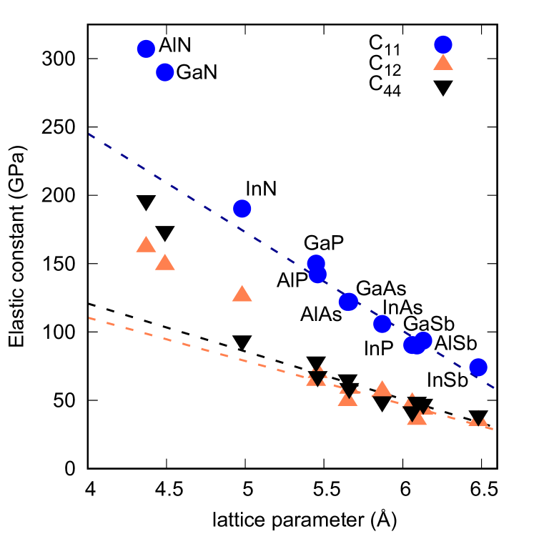
Figure 3: Dependence of elastic constants on the equilibrium lattice parameter. Elastic constants and lattice parameters have been obtained using $\text{HSE}_{\alpha}$ functional.

III.4 Band Structures

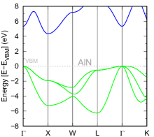
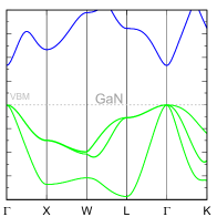
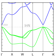
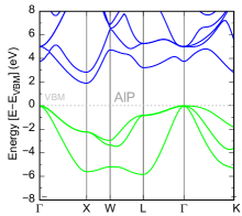
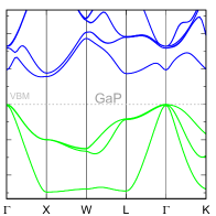
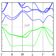
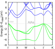
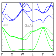
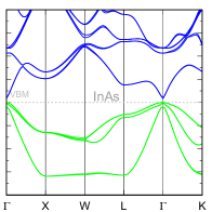
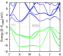
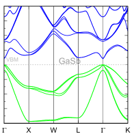
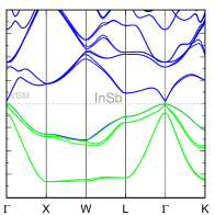
Figure 4: $\text{HSE}_{\alpha}$+SOC band structures obtained. Energy zero is set to the valence band maximum (VBM). Blue and green lines indicate conduction and valence bands, respectively.

As discussed previously,Perdew and Levy (1983); Kim et al. (2010) the PBE functional strongly underestimates the band gap energy. In the specific case of the small band gap III-V materials, leading to results presenting a null band gap or even the inversion of the ordering of $\Gamma_{6}$ and $\Gamma_{8}$ states, as showed in Fig. 4b. This result is completely inconsistent with the experimental data.Madelung (2004); Vurgaftman et al. (2001) To get rid of this problem, we employed the HSE06 and $\text{HSE}_{\alpha}$ exchange and correlation functions. The differences on the results using the different functionals may be clarified by analyzing the results as shown in Figure 4. The HSE06 and HSE_α gaps are closer to the experimental values than PBE predictions, e.g., InP shows an increase of the value of $68\text{\,}\mathrm{\char 37\relax}$ from PBE to HSE_α. An even more dramatic example is the wrong predictions of negative band gaps for InSb, GaSb, InAs and InN made using the PBE functional. HSE06 or HSE_α functionals show the correct trend.

Although both HSE06 or HSE_α functionals predict the correct trend, the tuning of $\alpha$ provides a much better agreement for the band gap value, changing the deviations from the experimental results from $0.8\text{\,}\mathrm{\char 37\relax}$ (InP) up to $42.1\text{\,}\mathrm{\char 37\relax}$ (InSb) when using HSE06 to $0.3\text{\,}\mathrm{\char 37\relax}$ (AlN) and $10.5\text{\,}\mathrm{\char 37\relax}$ (InN) with HSE_α. The accuracy in the description of $\Delta_{\text{so}}$ is also improved when using the hybrid functionals instead of PBE, as shown in Table 3. The band structures for all the other materials are presented in the Supplementary Material.

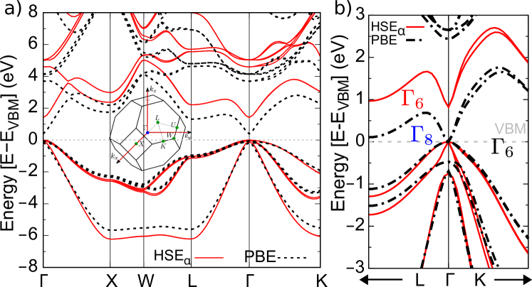
Figure 4: InP and GaSb band structures evaluated with PBE (dashed line) and $\text{HSE}_{\alpha}$ (solid line) including spin-orbit coupling. a) band structure for InP. The first Brillouin zone of zinc-blende phase is shown. b) GaSb band structure close to $\Gamma$ point: PBE presents a negative band gap and the $\text{HSE}_{\alpha}$ shows a positive band gap. The band symmetries are indicated.

Table 3: Band gap, $E_{\text{gap}}=\Gamma^{c}_{6}-\Gamma^{v}_{8}$, and spin-orbit splitting, $\Delta_{\text{so}}=\Gamma^{v}_{8}-\Gamma^{v}_{7}$, energies using the different functionals: PBE, PBE+SOC, HSE06, HSE06+SOC and $\text{HSE}_{\alpha}$+SOC. The contribution of nonlocal exchange in the HSE, $\alpha$, adjusted to obtain the experimental values of gap energy and spin-orbit splitting is also shown. The energies are given in $\mathrm{eV}$.

			PBE		PBE+SOC			HSE06		HSE06+SOC			$\text{HSE}_{\alpha}$+SOC			literature
	$\alpha$		$E_{\text{gap}}$		$E_{\text{gap}}$	$\Delta_{\text{so}}$		$E_{\text{gap}}$		$E_{\text{gap}}$	$\Delta_{\text{so}}$		$E_{\text{gap}}$	$\Delta_{\text{so}}$		$E_{\text{gap}}$	$\Delta_{\text{so}}$
AlN	$0.219$		$4.003$		$3.997$	$0.019$		$5.609$		$5.601$	$0.021$		$5.383$	$0.022$		$5.40$f	$0.019$f
AlP	$0.127$		$3.090$		$3.070$	$0.059$		$4.164$		$4.153$	$0.064$		$3.611$	$0.061$		$3.62$c	$0.06$b
AlAs	$0.343$		$1.757$		$1.662$	$0.290$		$2.819$		$2.732$	$0.316$		$3.157$	$0.324$		$3.13$c	$0.3$c
AlSb	$0.318$		$1.314$		$1.105$	$0.652$		$2.286$		$2.111$	$0.691$		$2.397$	$0.700$		$2.38$c	$0.673$c
GaN	$0.293$		$1.564$		$1.560$	$0.012$		$3.043$		$3.042$	$0.021$		$3.312$	$0.022$		$3.30$d	$0.017$f
GaP	$0.283$		$1.603$		$1.576$	$0.082$		$2.748$		$2.739$	$0.092$		$2.915$	$0.093$		$2.895$c	$0.08$f
GaAs	$0.318$		$0.166$		$0.072$	$0.325$		$1.297$		$1.210$	$0.358$		$1.471$	$0.365$		$1.519$c	$0.341$c
GaSb	$0.297$		$-0.259$		$-0.477$	$0.694$		$0.782$		$0.614$	$0.743$		$0.819$	$0.751$		$0.82$c	$0.756$c
InN	$0.274$		$-0.504$		$-0.497$	$0.002$		$0.507$		$0.530$	$0.016$		$0.674$	$0.017$		$0.61$g	$0.005$f
InP	$0.253$		$0.468$		$0.452$	$0.095$		$1.402$		$1.408$	$0.111$		$1.422$	$0.111$		$1.42$c	$0.108$c
InAs	$0.289$		$-0.525$		$-0.626$	$0.335$		$0.372$		$0.301$	$0.373$		$0.373$	$0.385$		$0.418$c	$0.38$c
InSb	$0.277$		$-0.558$		$-0.782$	$0.716$		$0.335$		$0.136$	$0.778$		$0.232$	$0.783$		$0.235$c	$0.81$c
NRMSD($\mathrm{\char 37\relax}$)			$55.7$		$59.1$	$12.0$		$9.1$		$10.9$	$4.8$		$1.3$	$5.4$

• Exp. from ref. Thompson et al., 2001,

• Theory GW from ref. Chantis et al., 2006,

• Exp. from ref. Madelung, 2004,

• Exp. from ref. Monemar, 1974,

• Exp. from ref. Walukiewicz et al., 2004,

• Theory from ref. Vurgaftman et al., 2001.

• Exp. from ref. Buß et al., 2015.

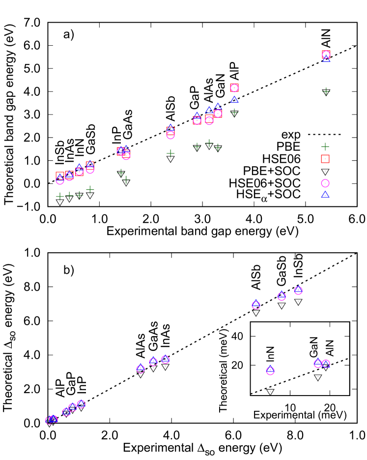
Figure 5: Energies of the $12$ compounds determined with the different functionals with and without the inclusion of the spin-orbit coupling: a) band gaps b) spin-orbit splittings. In both figures, the dashed lines show the literature values.

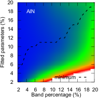
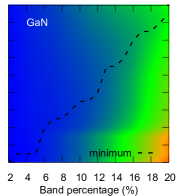
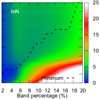
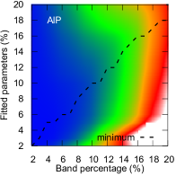
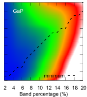
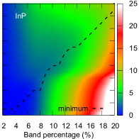
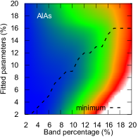
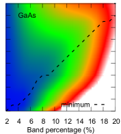
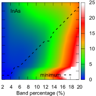
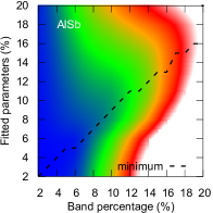
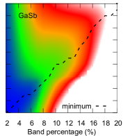
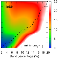
Figure 5: Density map showing the agreement of the different adjusted parameter sets against the range around the $\Gamma$-point they are sampled, using the Root mean square deviation (RMSD) measure. The dashed line indicate the optimal sets parameter.

Regardless of the gap adjustment, i.e., using the HSE06 calculations, one can notice a monotonic relation between the anionic radius and the band gap energies, e.g., in Al compounds, we observe that $E_{\text{gap}}^{\ce{AlN}}>E_{\text{gap}}^{\ce{AlP}}>E_{\text{gap}}^{\ce{AlAs}}>E_{\text{gap}}^{\ce{AlSb}}$. This trend is also valid for the As compounds, as shown in Fig. 5. It fails, however, for the In compounds, in which the calculated InN band gap is smaller than the trend suggests. Carrier et al.Carrier and Wei (2005) suggested, when this same rule was violated for wurtzite compounds, that this was due to the high electronegativity of N and the smaller band gap deformation potentials. In our understanding, the same explanation should be applied to the zinc-blende case.

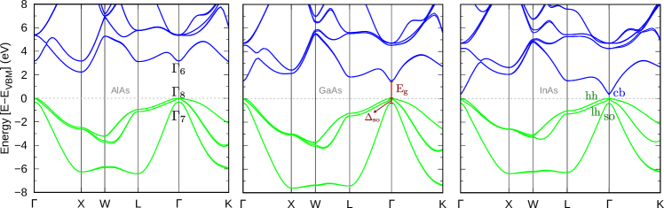
Figure 6: Band structures obtained using $\text{HSE}_{\alpha}$+SOC along high symmetry lines for AlAs, GaAs and InAs. The blue lines indicate conduction bands, while the green lines, the valence bands. The band structures for the other III-V materials are shown in the Supplementary Materials.

III.5 $\mathbf{k{\cdot}p}$ Parameters

Despite the fact that band gaps and $\Delta_{\text{so}}$ are close to the experimental values, there is no guarantee that the calculated band structures are in agreement with the experimental results. To perform this analysis, we calculated the effective masses, using the $\mathbf{k{\cdot}p}$ approach. In the $\mathbf{k{\cdot}p}$ method, the interactions involving electrons and nuclei are described through an effective potential with the same periodicity of the lattice, allowing the utilization of the Bloch’s theorem. To found an effective Hamiltonian, we used the perturbative technique proposed by Löwdin,Löwdin (1951) where the basis set is divided in two classes: A and B. States within the class A, are the states of interest and are described exactly, while states from the class B are taken into account perturbativelly through the interactions with the states of class A. Class A states are chosen according to the energy range at the point of the first Brillouin zone (FBZ) in aim, defining the effective Hamiltonian.

In this work, we used the $6{\times}6$ zinc-blende effective $\mathbf{k{\cdot}p}$ Hamiltonians proposed by Luttinger-Kohn Luttinger and Kohn (1955) (LK6) and extended by Kane to an $8{\times}8$ model.Kane (1966) In the LK6 model, in the vicinity of the $\Gamma$ point, the class A is composed by the three topmost valence bands, i.e., HH, LH and SO, and the matrix elements are determined using perturbation theory up to the second order. In the Kane model, the same bands and perturbative order were used but class A also includes the first conduction band (CB). The use the symmetry properties of zinc-blende crystals and some algebraic manipulationLok C. Lew Yan Voon (2009); Enderlein (1997) shows that the Kane Hamiltonian depend on $5$ different effective mass parameters $\tilde{\gamma}_{1}$, $\tilde{\gamma}_{2}$, $\tilde{\gamma}_{3}$, $\tilde{\text{e}}$ and $P$, plus the gap and $\Delta_{\text{so}}$, while the LK6 depends only on $3$ parameters, $\gamma_{1}$, ${\gamma}_{2}$ and ${\gamma}_{3}$, plus the $\Delta_{\text{so}}$. As the $\mathbf{k{\cdot}p}$ method is semi-empirical, all effective mass parameters are obtained, with little algebraic manipulations, from the direct measurements of the effective masses of the carriers in the materials, except for the $P$ parameter.

Distinctly from the other effective mass parameters, $P$ can not be obtained by direct measures, but must be extracted from the interband (CB-VB) interaction energy $E_{P}$. An accurate measure of $E_{P}$ is hard to obtain due to the inherent difficulties associated with the decoupling of the CB-VB interaction to the interaction of them with the remote bands. $E_{P}$ values have been estimated indirectly by experimental techniques such as electron-spin-resonance, through interband matrix elements.Weisbuch and Hermann (1977); Chadi et al. (1976) and from measures of the $g$-factors, which have small influence from the remote bands and yield more accurate values.Vurgaftman et al. (2001) Due to the difficulties involved in the measuring the $g$-factor in III-V semiconductors, the traditional procedure is to obtain the $P$ parameter from the effective mass parameters using the $6{\times}6$ $\mathbf{k{\cdot}p}$ Hamiltonian. When the $P$ is determined, the $8{\times}8$ parameters can be evaluated using the relations showed in appendix A.

We chose in this work an alternative method to determine the effective mass and $P$ parameters from band structures evaluated by DFT calculations. We fitted the HSE_α band structure using the secular equation of the $8{\times}8$ Hamiltonian proposed in the Ref. Bastos et al., 2016, determining simultaneously all the parameters. All points have the same weight and the same distance for all materials. Using different percentages of the FBZ around $\Gamma$ point, we determined different parameter sets and the choice of the final set of parameters was done by root mean square deviation (RMSD) analysis,Bastos et al. (2016) using the euclidean distance between the band structures from HSE_α and the effective Hamiltonian $\mathbf{k{\cdot}p}$ with the adjusted parameters. Technical details about the fitting are available in the Supplementary Material.

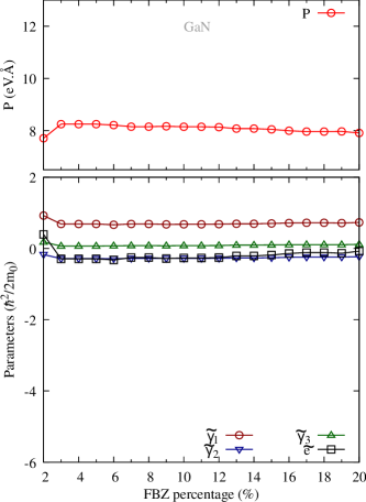
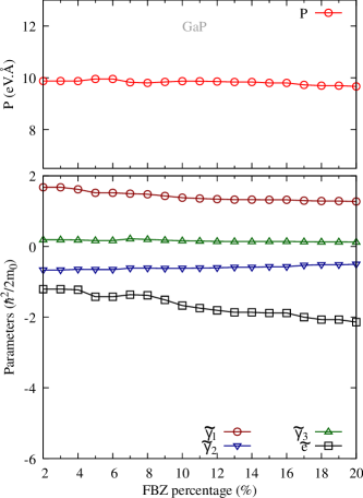
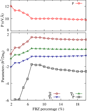
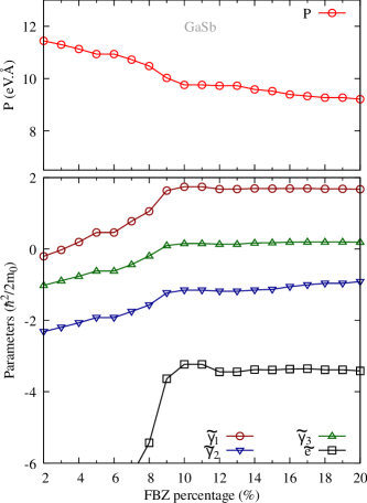
Figure 7: Recommended Kane parameters for each region near to $\Gamma$ point for gallium-V compounds. In the x-axis is the percentage of the FBZ used in the fitting.

As the difference between $\mathbf{k{\cdot}p}$ and HSE_α increases considerably for large FBZ percentages, we recommend the values from the fitting for $10\text{\,}\mathrm{\char 37\relax}$ as showed in Table IV. This choice is a compromise between describing a reasonable percentage of the band and obtaining a small deviation of HSE_α band structure. A general feature of the band structures is the non-parabolicity in the region between $6$ and $8\text{\,}\mathrm{\char 37\relax}$ of the FBZ, better seen on CB and SO bands, as showed in Fig. 7. Another non-parabolicity also arises near $15\text{\,}\mathrm{\char 37\relax}$. Depending on the magnitude of this second non-parabolicity in an specific direction, the deviations of the values become more or less important at $20\text{\,}\mathrm{\char 37\relax}$ of the FBZ.

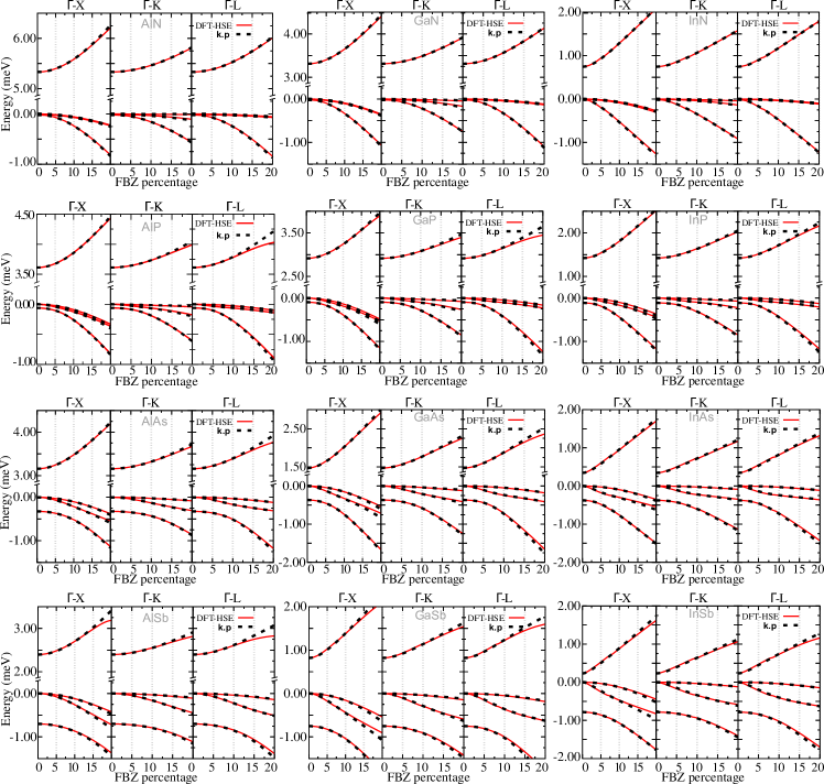
Figure 7: HSE_α and $\mathbf{k{\cdot}p}$ band structure comparisons. The optimal parameters were obtained from fitting using $10\text{\,}\mathrm{\char 37\relax}$ of the FBZ. Three high symmetry directions are shown: $\Gamma$-X, $\Gamma$-K and $\Gamma$-L.

Table 4: Kane and Luttinger–Kohn parameters obtained through the fitting of the Kane $\mathbf{k{\cdot}p}$ Hamiltonian in the band structure obtained using $\text{HSE}_{\alpha}$+SOC close to $\Gamma$ point. A range of Luttinger-Kohn parameters found in the compilation of the literature in references Madelung et al., 1982; Vurgaftman et al., 2001; Vurgaftman and Meyer, 2003 is given for comparison. The $\tilde{\gamma}_{s}$, ${\gamma}_{s}$, ẽ and e values are in $\hbar^{2}/2m_{0}$ units, while $\text{E}_{\text{p}}$ are in $\mathrm{eV}$.

	Kane					Luttinger-Kohn					range in literature for Luttinger-Kohn parameters
	$\tilde{\gamma}_{1}$	$\tilde{\gamma}_{2}$	$\tilde{\gamma}_{3}$	$\tilde{\text{e}}$	$E_{P}$		$\gamma_{1}$	$\gamma_{2}$	$\gamma_{3}$	e		$\gamma_{1}$	$\gamma_{2}$	$\gamma_{3}$	e	$E_{P}$
AlN	$0.36$	$-0.20$	$0.06$	$-0.10$	$18.8$		$1.52$	$0.38$	$0.64$	$3.38$		$1.92$	$0.47$	$0.85$	$3.03$-$4.0$	$27.1$
AlP	$0.81$	$-0.48$	$0.09$	$-1.01$	$22.1$		$2.85$	$0.54$	$1.11$	$5.07$		$3.35$-$3.47$	$0.06$-$0.71$	$1.15$-$1.19$	$4.55$	$17.7$
AlAs	$0.95$	$-0.61$	$0.06$	$-1.26$	$27.2$		$3.79$	$0.92$	$1.50$	$6.99$		$3.25$-$4.04$	$0.65$-$0.9$	$1.21$-$1.38$	$6.67$	$21.1$
AlSb	$0.89$	$-1.05$	$-0.11$	$-3.66$	$27.9$		$5.02$	$1.15$	$1.95$	$7.88$		$4.15$-$5.18$	$1.01$-$1.19$	$1.71$-$1.81$	$3.03$-$8.33$	$18.7$
GaN	$0.68$	$-0.28$	$0.08$	$-0.27$	$16.4$		$2.39$	$0.60$	$0.94$	$4.87$		$2.67$-$3.07$	$0.75$-$0.86$	$1.1$-$1.16$	$6.67$	$25$
GaP	$1.38$	$-0.62$	$0.16$	$-1.67$	$25.2$		$4.20$	$0.87$	$1.58$	$6.68$		$4.05$-$4.2$	$0.49$-$0.98$	$1.25$-$1.95$	$7.69$-$10.81$	$31.4$
GaAs	$1.37$	$-0.81$	$0.10$	$-2.02$	$25.9$		$7.10$	$2.15$	$2.99$	$14.05$		$6.8$-$7.8$	$2.02$-$2.50$	$1.0$-$2.43$	$14.93$-$15.43$	$25.9$-$27.6$
GaSb	$1.74$	$-1.15$	$0.15$	$-3.23$	$24.8$		$11.78$	$3.87$	$5.19$	$22.04$		$11.08$-$13.4$	$4.03$-$4.7$	$5.26$-$5.74$	$24.27$-$25.64$	$23.7$-$25.1$
InN	$0.65$	$-0.25$	$0.05$	$-0.16$	$11.1$		$6.13$	$2.49$	$2.79$	$16.15$		$3.72$	$1.26$	$1.63$	$8.33$-$14.29$	$17.2$-$21.1$
InP	$1.23$	$-0.54$	$0.14$	$-1.18$	$18.3$		$5.33$	$1.58$	$2.20$	$10.86$		$4.95$-$6.28$	$0.94$-$2.08$	$1.62$-$2.08$	$12.38$-$14.71$	$18.1$-$19.6$
InAs	$1.29$	$-0.77$	$0.10$	$-1.38$	$18.9$		$18.20$	$7.69$	$8.55$	$40.75$		$19.67$-$20.5$	$8.30$-$8.50$	$9.10$-$9.17$	$37.74$-$45.66$	$21.5$-$21.9$
InSb	$1.68$	$-1.04$	$0.12$	$-2.09$	$20.4$		$31.05$	$13.65$	$14.80$	$63.37$		$34.5$-$37.1$	$14.5$-$16.5$	$15.7$-$17.7$	$68.49$-$84.75$	$23.1$-$23.5$

In Table 4, we show the values for Kane ($\tilde{\gamma}_{1}$, $\tilde{\gamma}_{2}$, $\tilde{\gamma}_{3}$, ẽ and $E_{P}$), and Luttinger–Kohn ($\gamma_{1}$, $\gamma_{2}$, $\gamma_{3}$ and e) parameters, determined with the data using the range of up to $10\text{\,}\mathrm{\char 37\relax}$ of the FBZ (and in any up to range from $2\text{\,}$ to $20\text{\,}\mathrm{\char 37\relax}$ in the Supplementary Materials). The ranges of the values observed in literature are also given for comparison. Due to the small number of results founded in the literature, we included both, experimental and theoretical works, indicating the maximum and minimum values extracted from traditional sources such as Madelung et al.,Madelung et al. (1982) Vurgaftman et al.Vurgaftman et al. (2001); Vurgaftman and Meyer (2003) and Winkler.Winkler (2003) Our results are in agreement with the literature, i.e., the obtained effective mass parameters are inside the range of the most accepted values. In addition, the highest deviation comes from the nitrides. Since the most stable phase for the III-nitrides is wurtzite and not zinc-blende, the scarce experimental data on it, prevents a more controlled comparison.

On the Kane models, the $P$ parameter, or its related energy $E_{P}$ is essential. This parameter represents the influence of the conduction band on the masses of the valence states and consequently the influence of the valence band on the conduction states. Our results for the $E_{P}$ parameter differ from the literature ones. The main reason for this difference is a divergence on the interpretation of the influence of the remote bands on the experimental measurements of the electron spin resonance as pointed out by Shantharama et al..Shantharama et al. (1984); Adams et al. In their article they compare, e.g., Chadi et al.Chadi et al. (1976) value for GaAs of $E_{P}=$29\text{\,}\mathrm{eV}$$ with their estimation based on an analysis of a $14{\times}14$ $\mathbf{k{\cdot}p}$ Hamiltonian of $E_{P}=$25.0(5)\text{\,}\mathrm{eV}$$. The reason for the divergence is atributed to an overestimation of the influence of the remote bands. Our suggested value for this parameter is $E_{P}=$25.9\text{\,}\mathrm{eV}$$. As $E_{P}$ is directly related to the Kane parameter $P$, its fitting is essential.

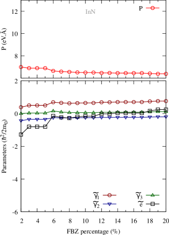
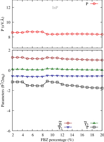
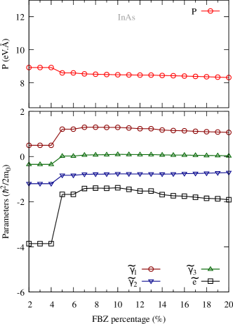
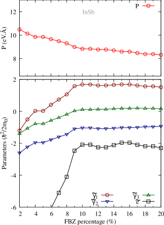
Figure 8: Recommended Kane parameters for each region near to $\Gamma$ point for Indium-V compounds. In the x-axis is the percentage of the FBZ used in the fitting.

As we have previously shown,Bastos et al. (2016) to correctly assign a value to $P$, it is necessary to include the first non-parabolicity in the range used for the fitting. If only the values below it are included, there is a fast variation of the values of $P$ depending on the range used. However, the fittings done with ranges including the non-parabolicity show a stabilization of the value. As an example, in Fig. 8. we present a curve of the fitted parameter for GaAs, showing the fast variation for ranges very close to the $\Gamma$-point and the stabilized values for ranges above $8\text{\,}\mathrm{\char 37\relax}$. The stabilization of our values suggests that our method improves the evaluation of the $P$ parameter, providing a way to distinguish the interactions of near and distant bands in the effective mass tensor. In the Supplementary Materials we provide the stabilization curves for the $P$, as well as the effective mass parameters, for all the materials.

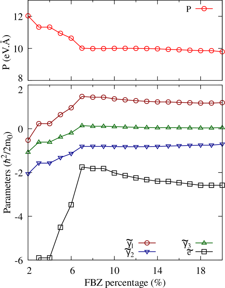
Figure 8: GaAs dependence of $P$ and Kane parameters with FBZ region used in the fitting process.

III.6 Effective mass and $g$-factors

In order to verify the accuracy of our calculations, we compared the experimental effective masses with the ones obtained from our effective mass parameters (see relations in Appendix A). Using the electronic $g$-factors, that are directly related to the spin splitting of the carrier bands, we have compared the measured values in the literature with our own values estimated from the $\mathbf{k{\cdot}p}$ parameters using the Roth’s formula,Roth et al. (1959)

$$\text{g}^{*}_{\text{c}}=2-\frac{2\text{E}_{\text{p}}\Delta_{\text{so}}}{3\text{E}_{\text{gap}}(\text{E}_{\text{gap}}+\Delta_{\text{so}})}\text{,}$$ (4)

and the values for $E_{P}$, $E_{gap}$ and ${\Delta}_{\text{so}}$. This equation includes only the interaction between VB and CB, while the interactions between the other bands are neglected.

Table 5 shows the effective masses and $g$-factors obtained by the $\mathbf{k{\cdot}p}$ parameters calculation. SO and CB electronic effective masses are considered to be isotropic and HH and LH were evaluated along three different directions of the FBZ: [111], [110] and [100]. The CB $g$-factors have been estimated using equation 4. Tabulated values, extracted from Refs. Madelung et al., 1982; Vurgaftman et al., 2001; Vurgaftman and Meyer, 2003; Martienssen and Warlimont, 2005 are presented for comparison. The Supplementary Material provides tables for all calculated parameter sets.

Table 5: Effective masses for light and the heavy hole along three directions ([100], [110] and [111]), isotropic masses from conduction band electrons and spin-orbit splitting holes and electron $g$-factors, obtained around the $\Gamma$ point, from the Luttinger-Kohn parameters. The ranges of values comprising the values found in the literature (experimental and theoretical results) are also shown for comparison.

		[100]			[110]			[111]
		$\text{m}_{\text{HH}}^{*}$	$\text{m}_{\text{LH}}^{*}$		$\text{m}_{\text{HH}}^{*}$	$\text{m}_{\text{LH}}^{*}$		$\text{m}_{\text{HH}}^{*}$	$\text{m}_{\text{LH}}^{*}$	$\text{m}_{\text{so}}^{*}$	$\text{m}_{\text{e}}^{*}$	$\text{g}_{\text{c}}^{*}$
AlN	this work	$1.320$	$0.437$		$4.123$	$0.357$		$2.858$	$0.371$	$0.659$	$0.296$	$1.99$
	literature										$0.330$a
AlP	this work	$0.563$	$0.255$		$1.599$	$0.197$		$1.176$	$0.206$	$0.355$	$0.197$	$1.93$
	literature	$0.513$b	$0.211$b					$1.372$b	$0.145$b	$0.30$a
AlAs	this work	$0.503$	$0.177$		$0.955$	$0.152$		$1.253$	$0.146$	$0.282$	$0.143$	$1.46$
	literature	$0.409$c	$0.153$c					$1.022$c	$0.109$c	$0.28$a	$0.15$c
AlSb	this work	$0.359$	$0.136$		$0.682$	$0.115$		$0.890$	$0.111$	$0.240$	$0.127$	$0.20$
	literature	$0.336$c	$0.123$c					$0.872$c	$0.091$c		$0.14$a
GaN	this work	$0.841$	$0.279$		$1.542$	$0.243$		$1.991$	$0.234$	$0.421$	$0.205$	$1.98$
	literature											$1.95$d
GaP	this work	$0.405$	$0.168$		$0.754$	$0.141$		$0.966$	$0.136$	$0.243$	$0.150$	$1.82$
	literature							$0.670$c	$0.170$c	$0.465$e	$0.13$a
GaAs	this work	$0.357$	$0.088$		$0.672$	$0.079$		$0.898$	$0.076$	$0.169$	$0.071$	$-0.34$
	literature	$0.34$b	$0.094$b					$0.75$b	$0.082$b		$0.0662$b	$-0.44$f
GaSb	this work	$0.247$	$0.051$		$0.500$	$0.046$		$0.710$	$0.045$	$0.144$	$0.045$	$-7.66$
	literature	$0.29$c			$0.36$c			$0.40$c		$0.12$a	$0.039$b	$-9.1$c
InN	this work	$0.874$	$0.090$		$1.851$	$0.085$		$1.460$	$0.086$	$0.167$	$0.062$	$1.73$
	literature
InP	this work	$0.460$	$0.118$		$0.828$	$0.106$		$1.073$	$0.103$	$0.199$	$0.092$	$1.38$
	literature									$0.121$b	$0.0808$b	1.48b
InAs	this work	$0.354$	$0.030$		$0.911$	$0.028$		$0.661$	$0.029$	$0.104$	$0.025$	$-15.18$
	literature	$0.35$b						$0.85$b		$0.14$a	$0.0265$b	$-15.3$b
InSb	this work	$0.266$	$0.017$		$0.498$	$0.017$		$0.692$	$0.016$	$0.119$	$0.016$	$-43.30$
	literature	$0.32$c			$0.42$c			$0.44$c		$0.11$a	$0.013$ b	$-51.31$b

• Theory from ref. Vurgaftman et al., 2001,

• Exp. from ref. Madelung, 2004,

• Exp. from ref. Martienssen and Warlimont, 2005,

• Exp. from ref. Buß et al., 2015,

• Theory from ref. Martienssen and Warlimont, 2005,

• Exp. from ref. Oestreich and Rühle, 1995.

As we can distinguish the effects of the interactions from inner and outer bands, our $g$-factors show excellent agreement with the literature values, exception done to the materials with large spin-orbit coupling, such as antimonides and indium compounds. In these materials we have found large deviations from the reference values of HH and LH effective masses along the [110] and [111] directions. The lack of $k$ dependence on the spin-orbit coupling on the $\mathbf{k{\cdot}p}$ Hamiltonian used in our description may be responsible for such deviation. However, even for these materials, the LH and HH $g$-factors along the [100] direction present good agreement with the experimental values, since the specific symmetry of the zinc-blende systems prevent the splitting of the bands along that specific direction. Finally, CB and SO bands also present good agreement with the experimental values, since the spin split for them is small.

IV Summary and conclusion

We reported an extensive ab initio study of electronic and structural properties of the III-V semiconductors ($12$ systems) based on DFT within the PBE, PBE+SOC, HSE06, HSE_α, and HSE_α+SOC functionals. For the hybrid HSE_α functional, we fitted the magnitude of the nonlocal Fock exchange that replaces part of the PBE exchange based on the experimental results for the fundamental band gap and spin-orbit splitting energies. Except for the AlP compound, whose $\alpha$ is $0.127$, our $\alpha$ parameters are in between $0.209$ and $0.343$, deviating less than $0.1$ from the universal value of $0.25$ estimated by Perdew.Perdew et al. (1996a)

Although the electronic properties were improved by the fitting, our results and analysis indicate clearly that HSE_α does not yield a significant improvement of the structural properties when compared with HSE06. In fact, it is an excellent result as it shows that is possible to improve the electronic properties without affecting the structural parameters by using fitted HSE_α functionals. This conclusion is valid, at least, for small changes in $\alpha$ near to the $0.25$ value. Furthermore, based on several analysis, we found a correlation between the values of $\alpha$ with the cationic radius, namely, the optimized $\alpha$ value descreases almost linearly as a function of the atomic cationic radius, except for the case of AlN. Therefore, our findings combined with previous results obtained by Viñes et al.Viñes et al. (2017) suggested that is possible to correlate the values of the ${\alpha}$ with the physical properties, and hence, it opens new possibilities in the study of much more complex materials.

We found that the HSE_α overestimates the elastic constants, while PBE underestimates them. However, the magnitude of the relative error is smaller employing the HSE_α functional. We obtained from our results that the elastic constants decrease as the ionic radius increase, and hence, the elastic constants decrease by increasing the lattice parameter of the crystal structures. This behavior was reported in the literatureAdachi (1992); Keyes (1962) and was traditionally used to estimate the elastic constantsWillardson and Beer (1975); Adachi (1985) by the extrapolation of the data.

In order to provide a deeper understanding of the band structure curvatures, we used the DFT band structures to determine accurate $\mathbf{k{\cdot}p}$ parameters, and, from them, obtained the effective masses and the $g$-factors beyond the parabolic model. For the antimonides and indium compounds in specific directions, we observed large deviations of the $g$-factors from the experimental results indicating that the $8{\times}8$ $\mathbf{k{\cdot}p}$ Hamiltonian may still not be adequate for describing systems with small band gap or large spin-orbit splittings. The $k$-dependent spin-orbit term, responsible for the spin-orbit splitting outside of the $\Gamma$ point, is neglected in our model, resulting in the deviations observed. Finally, we tabulated the effective masses and $\mathbf{k{\cdot}p}$ parameters, presenting a full set of III-V parameters that may be used in realistic simulations of systems with higher complexity, such as nanowires and quantum dots, or devices based on these compounds.

Appendix A Luttinger–Kohn Parameters and Effective mass Relations

Since class A and B states differ among the $6\times 6$ and $8\times 8$ models, the definitions of the effective mass parameters differ from one model to the other.Enderlein (1997); Lok C. Lew Yan Voon (2009) The relation among both model parameters, for zinc-blende structures, is given by the following expressions

$$\begin{split}\gamma_{1}=&\tilde{\gamma}_{1}+\frac{\text{E}_{\text{p}}}{3\text{E}_{\text{gap}}},\hskip 14.22636pt\gamma_{2}=\tilde{\gamma}_{2}+\frac{\text{E}_{\text{p}}}{6\text{E}_{\text{gap}}},\\ \gamma_{3}=&\tilde{\gamma}_{3}+\frac{\text{E}_{\text{p}}}{6\text{E}_{\text{gap}}},\hskip 18.49411pte=\tilde{e}+\frac{(\text{E}_{\text{gap}}+\frac{2}{3}\Delta_{\text{so}})\text{E}_{\text{p}}}{\text{E}_{\text{gap}}(\text{E}_{\text{gap}}+\Delta_{\text{so}})},\\ \text{E}_{\text{p}}=&\frac{2\text{m}_{0}}{\hbar^{2}}\text{P}^{2}.\end{split}$$

The effective masses may be determined from the parameters using the following relations

$$\begin{split}\text{m}_{\text{lh}[100]}=&(\gamma_{1}+2\gamma_{2})^{-1},\\ \text{m}_{\text{hh}[100]}=&(\gamma_{1}-2\gamma_{2})^{-1},\\ \text{m}_{\text{e}}=&e^{-1},\end{split}\quad\begin{split}\text{m}_{\text{lh}[110]}=&(\gamma_{1}+2\gamma_{3})^{-1},\\ \text{m}_{\text{hh}[110]}=&(\gamma_{1}-2\gamma_{3})^{-1},\\ \text{m}_{\text{lh}[111]}=&(\gamma_{1}+\sqrt{\gamma_{2}^{2}+3\gamma_{3}^{2}})^{-1},\end{split}$$

$$\begin{split}\text{m}_{\text{hh}[111]}=&(\gamma_{1}-\sqrt{\gamma_{2}^{2}+3\gamma_{3}^{2}})^{-1},\\ \text{m}_{\text{so}}=&\left(\gamma_{1}-\frac{1}{3}\frac{\Delta_{\text{so}}\text{E}_{\text{p}}}{\text{E}_{\text{gap}}(\text{E}_{\text{gap}}+\Delta_{\text{so}})}\right)^{-1}.\end{split}$$

Appendix B Effective Bader Charge

Table 6: Effective Bader charge evaluated using the PBE functional for III-V semiconductors. All units are in $\mathrm{C}$.

	N	P	As	Sb
Al	$2.37$	$2.06$	$1.92$	$1.63$
Ga	$1.52$	$0.84$	$0.68$	$0.34$
In	$1.40$	$0.88$	$0.74$	$0.47$

Supplementary Material: A comprehensive study of g-factors, elastic, structural and electronic properties of III-V semiconductors using Hybrid-Density Functional Theory

I Computational details

Table 1: HSE functional PAW VASP projectors used in this work, together with the number of valence electrons (ZVAL) and the cut-off energies recommended by VASP, used in the minimization of the stress/elastic constants tensor and in the determination of the total energy/band structures.

					cut-off energy ($\mathrm{eV}$)
		PAW	ZVAL	valence	recommended		stress/elastic constants		total energy/band structure
Al		Al_GW_19Mar2012	3	3s${}^{\text{2}}$ 3p${}^{\text{1}}$	240.300		360.450		270.337
Ga		Ga_d_GW_06Jul2010	3	4s${}^{\text{2}}$ 4p${}^{\text{1}}$	134.678		202.017		151.513
In		In_d_GW_29May2007	13	4d${}^{\text{10}}$ 5s${}^{\text{2}}$ 5p${}^{\text{1}}$	278.624		417.936		313.452
N		N_GW_10Apr2007	5	2s${}^{\text{2}}$ 2p${}^{\text{3}}$	420.902		631.353		473.515
P		P_GW_19Mar2012	5	3s${}^{\text{2}}$ 3p${}^{\text{3}}$	255.040		382.560		286.920
As		As_GW_20Mar2012	5	4s${}^{\text{2}}$ 4p${}^{\text{3}}$	208.702		313.053		234.790
Sb		Sb_d_GW_22Apr2009	15	4d${}^{\text{10}}$ 5s${}^{\text{2}}$ 5p${}^{\text{3}}$	172.069		258.103		193.578

Table 2: PBE functional PAW VASP projectors used in this work, together with the number of valence electrons (ZVAL) and the cut-off energies recommended by VASP, used in the minimization of the stress/elastic constants tensor and in the determination of the total energy/band structures.

					cut-off energy ($\mathrm{eV}$)
		PAW	ZVAL	valence	recommended		stress	elastic constants	total energy/band structure
Al		Al_GW_19Mar2012	3	3s${}^{\text{2}}$ 3p${}^{\text{1}}$	240.300		480.600	600.750	270.337
Ga		Ga_d_GW_06Jul2010	3	4s${}^{\text{2}}$ 4p${}^{\text{1}}$	134.678		269.356	336.695	151.513
In		In_d_GW_29May2007	13	4d${}^{\text{10}}$ 5s${}^{\text{2}}$ 5p${}^{\text{1}}$	278.624		557.248	696.560	313.452
N		N_GW_10Apr2007	5	2s${}^{\text{2}}$ 2p${}^{\text{3}}$	420.902		841.804	1052.255	473.515
P		P_GW_19Mar2012	5	3s${}^{\text{2}}$ 3p${}^{\text{3}}$	255.040		510.080	637.600	286.920
As		As_GW_20Mar2012	5	4s${}^{\text{2}}$ 4p${}^{\text{3}}$	208.702		417.404	521.755	234.790
Sb		Sb_d_GW_22Apr2009	15	4d${}^{\text{10}}$ 5s${}^{\text{2}}$ 5p${}^{\text{3}}$	172.069		344.138	430.172	193.578

II Dependence of properties with parameters

II.1 Dependence of the band gap and $\Delta_{\text{so}}$ on the $\alpha$ parameter

II.2 $\alpha$ parameters

III Band Structures

IV $\mathbf{k\cdot p}$ parameters

V Kane parameters

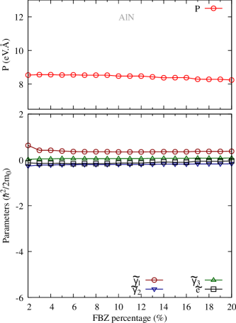
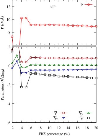
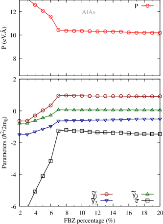
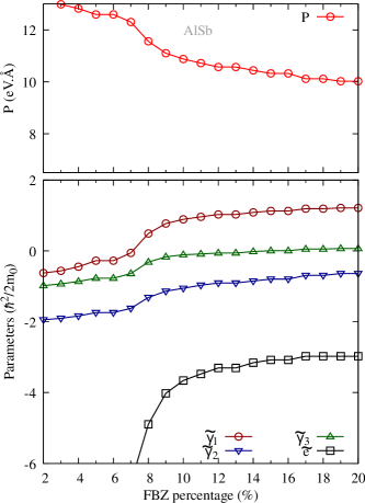
Figure 6: Recommended Kane parameters for each region near to $\Gamma$ point for aluminum-V compounds. In the x-axis is the percentage of the FBZ used in the fitting.

VI Kane-Lutinger parameters

Table 3: Adjusted Kane parameters and $\text{E}_{\text{p}}$ for AlN and AlP in function of the adjusted region. The RMSDs are also indicated.

	AlN						AlP
$\mathrm{\char 37\relax}$	RMSD	$\tilde{\gamma}_{1}$	$\tilde{\gamma}_{2}$	$\tilde{\gamma}_{3}$	ẽ	P	RMSD	$\tilde{\gamma}_{1}$	$\tilde{\gamma}_{2}$	$\tilde{\gamma}_{3}$	ẽ	P
$2$	$0.35$	$0.439$	$-0.228$	$0.006$	$-0.049$	$8.44$	$0.19$	$1.627$	$-0.278$	$0.272$	$1.453$	$7.32$
$3$	$0.37$	$0.399$	$-0.221$	$0.022$	$-0.101$	$8.49$	$0.18$	$1.627$	$-0.278$	$0.272$	$1.453$	$7.32$
$4$	$0.44$	$0.365$	$-0.206$	$0.048$	$-0.113$	$8.49$	$0.20$	$0.392$	$-0.742$	$-0.161$	$-2.248$	$10.20$
$5$	$0.52$	$0.358$	$-0.204$	$0.051$	$-0.119$	$8.49$	$0.26$	$0.392$	$-0.742$	$-0.161$	$-2.248$	$10.20$
$6$	$0.61$	$0.358$	$-0.204$	$0.051$	$-0.119$	$8.49$	$0.49$	$0.861$	$-0.485$	$0.094$	$-0.833$	$9.16$
$7$	$0.75$	$0.362$	$-0.198$	$0.060$	$-0.099$	$8.45$	$0.71$	$0.861$	$-0.485$	$0.094$	$-0.833$	$9.16$
$8$	$0.85$	$0.362$	$-0.198$	$0.060$	$-0.099$	$8.45$	$1.01$	$0.846$	$-0.479$	$0.089$	$-0.887$	$9.14$
$9$	$1.00$	$0.362$	$-0.198$	$0.060$	$-0.099$	$8.45$	$1.41$	$0.826$	$-0.484$	$0.081$	$-0.946$	$9.16$
$10$	$1.20$	$0.362$	$-0.198$	$0.060$	$-0.099$	$8.45$	$1.89$	$0.810$	$-0.484$	$0.075$	$-1.010$	$9.17$
$11$	$1.45$	$0.362$	$-0.198$	$0.060$	$-0.099$	$8.45$	$2.71$	$0.810$	$-0.484$	$0.075$	$-1.010$	$9.17$
$12$	$1.64$	$0.360$	$-0.196$	$0.062$	$-0.097$	$8.44$	$3.55$	$0.796$	$-0.464$	$0.076$	$-1.107$	$9.14$
$13$	$1.99$	$0.360$	$-0.196$	$0.062$	$-0.097$	$8.44$	$4.33$	$0.796$	$-0.464$	$0.076$	$-1.107$	$9.14$
$14$	$2.38$	$0.365$	$-0.188$	$0.070$	$-0.076$	$8.39$	$5.49$	$0.797$	$-0.442$	$0.082$	$-1.145$	$9.08$
$15$	$2.72$	$0.358$	$-0.189$	$0.069$	$-0.094$	$8.40$	$6.79$	$0.796$	$-0.431$	$0.081$	$-1.177$	$9.04$
$16$	$3.09$	$0.358$	$-0.189$	$0.069$	$-0.094$	$8.40$	$8.31$	$0.795$	$-0.418$	$0.081$	$-1.213$	$9.01$
$17$	$3.65$	$0.376$	$-0.177$	$0.079$	$-0.042$	$8.31$	$10.71$	$0.795$	$-0.418$	$0.081$	$-1.213$	$9.01$
$18$	$4.11$	$0.372$	$-0.176$	$0.077$	$-0.053$	$8.31$	$12.84$	$0.795$	$-0.398$	$0.083$	$-1.253$	$8.96$
$19$	$4.73$	$0.379$	$-0.171$	$0.081$	$-0.036$	$8.26$	$14.78$	$0.792$	$-0.386$	$0.081$	$-1.301$	$8.92$
$20$	$5.34$	$0.379$	$-0.171$	$0.081$	$-0.036$	$8.26$	$17.36$	$0.792$	$-0.386$	$0.081$	$-1.301$	$8.92$

Table 4: Adjusted Kane parameters and $\text{E}_{\text{p}}$ for AlAs and AlSb in function of the adjusted region. The RMSDs are also indicated.

	AlAs						AlSb
$\mathrm{\char 37\relax}$	RMSD	$\tilde{\gamma}_{1}$	$\tilde{\gamma}_{2}$	$\tilde{\gamma}_{3}$	ẽ	P	RMSD	$\tilde{\gamma}_{1}$	$\tilde{\gamma}_{2}$	$\tilde{\gamma}_{3}$	ẽ	P
$2$	$0.02$	$-0.636$	$-1.493$	$-0.779$	$-6.117$	$13.10$	$0.02$	$-0.625$	$-1.944$	$-0.981$	$-8.268$	$13.08$
$3$	$0.05$	$-0.636$	$-1.493$	$-0.779$	$-6.117$	$13.10$	$0.04$	$-0.562$	$-1.904$	$-0.929$	$-8.037$	$12.98$
$4$	$0.10$	$-0.295$	$-1.313$	$-0.605$	$-5.074$	$12.58$	$0.10$	$-0.445$	$-1.836$	$-0.863$	$-7.681$	$12.82$
$5$	$0.18$	$0.031$	$-1.144$	$-0.439$	$-4.090$	$12.08$	$0.24$	$-0.277$	$-1.743$	$-0.772$	$-7.193$	$12.59$
$6$	$0.51$	$0.342$	$-0.982$	$-0.277$	$-3.154$	$11.58$	$0.43$	$-0.277$	$-1.743$	$-0.772$	$-7.193$	$12.59$
$7$	$0.86$	$0.953$	$-0.638$	$0.070$	$-1.250$	$10.43$	$1.23$	$-0.057$	$-1.622$	$-0.639$	$-6.554$	$12.30$
$8$	$1.06$	$0.967$	$-0.621$	$0.064$	$-1.203$	$10.36$	$2.18$	$0.491$	$-1.315$	$-0.315$	$-4.895$	$11.56$
$9$	$1.49$	$0.951$	$-0.609$	$0.060$	$-1.262$	$10.35$	$2.78$	$0.772$	$-1.139$	$-0.169$	$-4.021$	$11.10$
$10$	$1.87$	$0.951$	$-0.609$	$0.060$	$-1.262$	$10.35$	$3.60$	$0.890$	$-1.054$	$-0.108$	$-3.660$	$10.87$
$11$	$2.49$	$0.935$	$-0.593$	$0.060$	$-1.320$	$10.32$	$4.60$	$0.963$	$-0.969$	$-0.087$	$-3.475$	$10.72$
$12$	$3.23$	$0.929$	$-0.581$	$0.058$	$-1.349$	$10.30$	$5.65$	$1.028$	$-0.907$	$-0.058$	$-3.305$	$10.57$
$13$	$4.15$	$0.929$	$-0.581$	$0.058$	$-1.349$	$10.30$	$7.16$	$1.028$	$-0.907$	$-0.058$	$-3.305$	$10.57$
$14$	$5.08$	$0.923$	$-0.567$	$0.057$	$-1.378$	$10.28$	$8.81$	$1.086$	$-0.851$	$-0.019$	$-3.157$	$10.44$
$15$	$6.43$	$0.923$	$-0.567$	$0.057$	$-1.378$	$10.28$	$10.90$	$1.127$	$-0.796$	$0.004$	$-3.076$	$10.32$
$16$	$8.02$	$0.920$	$-0.534$	$0.061$	$-1.415$	$10.21$	$13.64$	$1.127$	$-0.796$	$0.004$	$-3.076$	$10.32$
$17$	$10.35$	$0.913$	$-0.517$	$0.058$	$-1.459$	$10.19$	$16.10$	$1.192$	$-0.691$	$0.052$	$-2.973$	$10.11$
$18$	$12.53$	$0.913$	$-0.517$	$0.058$	$-1.459$	$10.19$	$19.36$	$1.192$	$-0.691$	$0.052$	$-2.973$	$10.11$
$19$	$14.77$	$0.913$	$-0.517$	$0.058$	$-1.459$	$10.19$	$22.64$	$1.213$	$-0.640$	$0.067$	$-2.973$	$10.02$
$20$	$17.60$	$0.913$	$-0.517$	$0.058$	$-1.459$	$10.19$	$25.94$	$1.213$	$-0.640$	$0.067$	$-2.973$	$10.02$

Table 5: Adjusted Kane parameters and $\text{E}_{\text{p}}$ for GaN and GaP in function of the adjusted region. The RMSDs are also indicated.

	GaN						GaP
$\mathrm{\char 37\relax}$	RMSD	$\tilde{\gamma}_{1}$	$\tilde{\gamma}_{2}$	$\tilde{\gamma}_{3}$	ẽ	P	RMSD	$\tilde{\gamma}_{1}$	$\tilde{\gamma}_{2}$	$\tilde{\gamma}_{3}$	ẽ	P
$2$	$0.02$	$0.922$	$-0.171$	$0.179$	$0.394$	$7.70$	$0.30$	$1.677$	$-0.665$	$0.190$	$-1.206$	$9.87$
$3$	$0.05$	$0.687$	$-0.285$	$0.067$	$-0.291$	$8.24$	$0.31$	$1.677$	$-0.665$	$0.190$	$-1.206$	$9.87$
$4$	$0.13$	$0.687$	$-0.285$	$0.067$	$-0.291$	$8.24$	$0.32$	$1.616$	$-0.648$	$0.183$	$-1.224$	$9.87$
$5$	$0.31$	$0.687$	$-0.285$	$0.067$	$-0.291$	$8.24$	$0.47$	$1.518$	$-0.653$	$0.169$	$-1.421$	$9.95$
$6$	$0.58$	$0.664$	$-0.287$	$0.074$	$-0.321$	$8.21$	$0.85$	$1.518$	$-0.653$	$0.169$	$-1.421$	$9.95$
$7$	$0.69$	$0.687$	$-0.278$	$0.080$	$-0.254$	$8.15$	$1.35$	$1.495$	$-0.614$	$0.218$	$-1.363$	$9.82$
$8$	$0.88$	$0.687$	$-0.278$	$0.080$	$-0.254$	$8.15$	$1.74$	$1.478$	$-0.615$	$0.201$	$-1.381$	$9.80$
$9$	$1.13$	$0.676$	$-0.281$	$0.076$	$-0.283$	$8.16$	$2.24$	$1.431$	$-0.621$	$0.178$	$-1.511$	$9.84$
$10$	$1.33$	$0.679$	$-0.278$	$0.080$	$-0.267$	$8.14$	$3.13$	$1.380$	$-0.618$	$0.163$	$-1.671$	$9.86$
$11$	$1.65$	$0.679$	$-0.278$	$0.080$	$-0.267$	$8.14$	$3.93$	$1.357$	$-0.612$	$0.153$	$-1.744$	$9.86$
$12$	$2.03$	$0.682$	$-0.275$	$0.083$	$-0.256$	$8.13$	$4.91$	$1.340$	$-0.602$	$0.146$	$-1.806$	$9.85$
$13$	$2.37$	$0.694$	$-0.265$	$0.094$	$-0.208$	$8.07$	$6.09$	$1.325$	$-0.589$	$0.140$	$-1.863$	$9.83$
$14$	$2.81$	$0.694$	$-0.265$	$0.094$	$-0.208$	$8.07$	$7.25$	$1.325$	$-0.589$	$0.140$	$-1.863$	$9.83$
$15$	$3.28$	$0.702$	$-0.259$	$0.099$	$-0.183$	$8.04$	$9.46$	$1.321$	$-0.573$	$0.143$	$-1.882$	$9.80$
$16$	$3.69$	$0.714$	$-0.248$	$0.106$	$-0.140$	$7.99$	$11.64$	$1.321$	$-0.573$	$0.143$	$-1.882$	$9.80$
$17$	$4.26$	$0.721$	$-0.241$	$0.110$	$-0.115$	$7.96$	$13.71$	$1.298$	$-0.532$	$0.136$	$-1.999$	$9.72$
$18$	$4.80$	$0.721$	$-0.241$	$0.110$	$-0.115$	$7.96$	$16.16$	$1.285$	$-0.518$	$0.131$	$-2.068$	$9.69$
$19$	$5.29$	$0.713$	$-0.240$	$0.106$	$-0.134$	$7.97$	$18.83$	$1.285$	$-0.518$	$0.131$	$-2.068$	$9.69$
$20$	$5.89$	$0.732$	$-0.228$	$0.115$	$-0.076$	$7.91$	$22.05$	$1.273$	$-0.504$	$0.127$	$-2.141$	$9.66$

Table 6: Adjusted Kane parameters and $\text{E}_{\text{p}}$ for GaAs and GaSb in function of the adjusted region. The RMSDs are also indicated.

	GaAs						GaSb
$\mathrm{\char 37\relax}$	RMSD	$\tilde{\gamma}_{1}$	$\tilde{\gamma}_{2}$	$\tilde{\gamma}_{3}$	ẽ	P	RMSD	$\tilde{\gamma}_{1}$	$\tilde{\gamma}_{2}$	$\tilde{\gamma}_{3}$	ẽ	P
$2$	$0.27$	$-0.521$	$-2.062$	$-1.065$	$-8.613$	$12.03$	$0.04$	$-0.205$	$-2.315$	$-1.020$	$-9.431$	$11.44$
$3$	$0.34$	$0.236$	$-1.569$	$-0.609$	$-5.899$	$11.32$	$0.12$	$-0.027$	$-2.196$	$-0.891$	$-8.785$	$11.29$
$4$	$0.44$	$0.236$	$-1.569$	$-0.609$	$-5.899$	$11.32$	$0.32$	$0.195$	$-2.069$	$-0.764$	$-8.086$	$11.13$
$5$	$0.57$	$0.645$	$-1.318$	$-0.371$	$-4.504$	$10.93$	$0.71$	$0.461$	$-1.923$	$-0.617$	$-7.278$	$10.93$
$6$	$1.38$	$0.961$	$-1.133$	$-0.184$	$-3.472$	$10.63$	$1.18$	$0.461$	$-1.923$	$-0.617$	$-7.278$	$10.93$
$7$	$2.00$	$1.477$	$-0.807$	$0.148$	$-1.749$	$10.01$	$2.52$	$0.776$	$-1.754$	$-0.437$	$-6.335$	$10.72$
$8$	$2.25$	$1.443$	$-0.804$	$0.117$	$-1.816$	$9.98$	$5.06$	$1.054$	$-1.571$	$-0.195$	$-5.430$	$10.48$
$9$	$2.75$	$1.443$	$-0.804$	$0.117$	$-1.816$	$9.98$	$6.53$	$1.635$	$-1.230$	$0.097$	$-3.636$	$10.02$
$10$	$3.46$	$1.368$	$-0.815$	$0.103$	$-2.020$	$9.99$	$7.69$	$1.743$	$-1.154$	$0.150$	$-3.232$	$9.75$
$11$	$4.23$	$1.322$	$-0.821$	$0.084$	$-2.140$	$10.00$	$8.57$	$1.743$	$-1.154$	$0.150$	$-3.232$	$9.75$
$12$	$5.23$	$1.284$	$-0.821$	$0.070$	$-2.245$	$9.99$	$9.65$	$1.677$	$-1.183$	$0.134$	$-3.442$	$9.72$
$13$	$6.40$	$1.254$	$-0.817$	$0.059$	$-2.328$	$9.98$	$11.41$	$1.677$	$-1.183$	$0.134$	$-3.442$	$9.72$
$14$	$7.54$	$1.229$	$-0.808$	$0.051$	$-2.398$	$9.97$	$13.54$	$1.694$	$-1.150$	$0.168$	$-3.380$	$9.58$
$15$	$9.12$	$1.226$	$-0.789$	$0.056$	$-2.406$	$9.93$	$15.74$	$1.690$	$-1.131$	$0.175$	$-3.388$	$9.52$
$16$	$10.84$	$1.207$	$-0.776$	$0.050$	$-2.464$	$9.91$	$18.28$	$1.693$	$-1.056$	$0.190$	$-3.365$	$9.39$
$17$	$12.76$	$1.190$	$-0.762$	$0.044$	$-2.523$	$9.88$	$20.52$	$1.694$	$-1.004$	$0.196$	$-3.354$	$9.33$
$18$	$15.30$	$1.175$	$-0.749$	$0.040$	$-2.582$	$9.85$	$23.25$	$1.683$	$-0.961$	$0.194$	$-3.385$	$9.27$
$19$	$18.04$	$1.175$	$-0.749$	$0.040$	$-2.582$	$9.85$	$26.15$	$1.683$	$-0.961$	$0.194$	$-3.385$	$9.27$
$20$	$21.48$	$1.194$	$-0.705$	$0.057$	$-2.581$	$9.78$	$28.79$	$1.674$	$-0.915$	$0.193$	$-3.416$	$9.21$

Table 7: Adjusted Kane parameters and $\text{E}_{\text{p}}$ for InN and InP in function of the adjusted region. The RMSDs are also indicated.

	InN						InP
$\mathrm{\char 37\relax}$	RMSD	$\tilde{\gamma}_{1}$	$\tilde{\gamma}_{2}$	$\tilde{\gamma}_{3}$	ẽ	P	RMSD	$\tilde{\gamma}_{1}$	$\tilde{\gamma}_{2}$	$\tilde{\gamma}_{3}$	ẽ	P
$2$	$0.75$	$0.388$	$-0.441$	$0.004$	$-1.280$	$6.99$	$0.03$	$1.277$	$-0.581$	$0.110$	$-1.156$	$8.60$
$3$	$0.86$	$0.498$	$-0.352$	$0.031$	$-0.805$	$6.89$	$0.04$	$1.277$	$-0.581$	$0.110$	$-1.156$	$8.60$
$4$	$0.97$	$0.498$	$-0.352$	$0.031$	$-0.805$	$6.89$	$0.07$	$1.277$	$-0.581$	$0.110$	$-1.156$	$8.60$
$5$	$1.27$	$0.498$	$-0.352$	$0.031$	$-0.805$	$6.89$	$0.14$	$1.159$	$-0.636$	$0.057$	$-1.515$	$8.71$
$6$	$2.92$	$0.691$	$-0.254$	$0.158$	$-0.145$	$6.64$	$0.29$	$1.160$	$-0.630$	$0.063$	$-1.510$	$8.69$
$7$	$3.51$	$0.651$	$-0.263$	$0.094$	$-0.231$	$6.58$	$0.85$	$1.149$	$-0.631$	$0.061$	$-1.541$	$8.69$
$8$	$3.69$	$0.623$	$-0.267$	$0.062$	$-0.279$	$6.55$	$2.13$	$1.149$	$-0.631$	$0.061$	$-1.541$	$8.69$
$9$	$3.74$	$0.639$	$-0.259$	$0.054$	$-0.197$	$6.51$	$2.64$	$1.264$	$-0.527$	$0.168$	$-1.085$	$8.37$
$10$	$3.79$	$0.648$	$-0.255$	$0.055$	$-0.161$	$6.50$	$2.95$	$1.227$	$-0.537$	$0.138$	$-1.182$	$8.37$
$11$	$3.87$	$0.648$	$-0.255$	$0.055$	$-0.161$	$6.50$	$3.30$	$1.227$	$-0.537$	$0.138$	$-1.182$	$8.37$
$12$	$4.04$	$0.689$	$-0.237$	$0.075$	$-0.019$	$6.46$	$3.74$	$1.149$	$-0.562$	$0.099$	$-1.396$	$8.39$
$13$	$4.17$	$0.689$	$-0.237$	$0.075$	$-0.019$	$6.46$	$4.24$	$1.110$	$-0.574$	$0.079$	$-1.507$	$8.40$
$14$	$4.33$	$0.704$	$-0.230$	$0.082$	$0.032$	$6.45$	$4.74$	$1.110$	$-0.574$	$0.079$	$-1.507$	$8.40$
$15$	$4.62$	$0.704$	$-0.230$	$0.082$	$0.032$	$6.45$	$5.49$	$1.087$	$-0.578$	$0.071$	$-1.567$	$8.40$
$16$	$4.85$	$0.704$	$-0.230$	$0.082$	$0.032$	$6.45$	$6.30$	$1.062$	$-0.582$	$0.060$	$-1.636$	$8.40$
$17$	$5.20$	$0.704$	$-0.230$	$0.082$	$0.032$	$6.45$	$7.23$	$1.043$	$-0.583$	$0.051$	$-1.690$	$8.39$
$18$	$5.56$	$0.739$	$-0.214$	$0.102$	$0.159$	$6.41$	$8.15$	$1.027$	$-0.582$	$0.044$	$-1.735$	$8.38$
$19$	$5.86$	$0.762$	$-0.201$	$0.114$	$0.241$	$6.38$	$9.40$	$1.023$	$-0.575$	$0.045$	$-1.744$	$8.36$
$20$	$6.29$	$0.762$	$-0.201$	$0.114$	$0.241$	$6.38$	$10.74$	$1.011$	$-0.570$	$0.041$	$-1.777$	$8.34$

Table 8: Adjusted Kane parameters and $\text{E}_{\text{p}}$ for InAs and InSb in function of the adjusted region. The RMSDs are also indicated.

	InAs						InSb
$\mathrm{\char 37\relax}$	RMSD	$\tilde{\gamma}_{1}$	$\tilde{\gamma}_{2}$	$\tilde{\gamma}_{3}$	ẽ	P	RMSD	$\tilde{\gamma}_{1}$	$\tilde{\gamma}_{2}$	$\tilde{\gamma}_{3}$	ẽ	P
$2$	$0.09$	$0.499$	$-1.202$	$-0.345$	$-3.857$	$8.92$	$0.29$	$-1.204$	$-2.604$	$-1.393$	$-10.959$	$10.48$
$3$	$0.12$	$0.499$	$-1.202$	$-0.345$	$-3.857$	$8.92$	$0.90$	$-0.508$	$-2.233$	$-1.062$	$-8.840$	$10.13$
$4$	$0.25$	$0.499$	$-1.202$	$-0.345$	$-3.857$	$8.92$	$1.66$	$0.028$	$-1.954$	$-0.775$	$-7.220$	$9.85$
$5$	$1.06$	$1.214$	$-0.831$	$0.022$	$-1.676$	$8.60$	$2.10$	$0.028$	$-1.954$	$-0.775$	$-7.220$	$9.85$
$6$	$1.20$	$1.214$	$-0.831$	$0.022$	$-1.676$	$8.60$	$2.93$	$0.410$	$-1.781$	$-0.569$	$-6.092$	$9.66$
$7$	$1.38$	$1.296$	$-0.785$	$0.068$	$-1.415$	$8.54$	$4.33$	$0.740$	$-1.607$	$-0.391$	$-5.099$	$9.48$
$8$	$1.64$	$1.299$	$-0.779$	$0.077$	$-1.396$	$8.52$	$7.01$	$1.062$	$-1.442$	$-0.187$	$-4.099$	$9.30$
$9$	$1.99$	$1.291$	$-0.776$	$0.082$	$-1.405$	$8.50$	$8.60$	$1.581$	$-1.100$	$0.034$	$-2.465$	$8.98$
$10$	$2.60$	$1.293$	$-0.766$	$0.097$	$-1.382$	$8.49$	$9.39$	$1.685$	$-1.037$	$0.120$	$-2.086$	$8.83$
$11$	$3.33$	$1.264$	$-0.770$	$0.093$	$-1.453$	$8.48$	$9.93$	$1.685$	$-1.037$	$0.120$	$-2.086$	$8.83$
$12$	$3.96$	$1.233$	$-0.772$	$0.087$	$-1.527$	$8.47$	$10.77$	$1.624$	$-1.082$	$0.132$	$-2.252$	$8.76$
$13$	$5.00$	$1.233$	$-0.772$	$0.087$	$-1.527$	$8.47$	$11.73$	$1.624$	$-1.082$	$0.132$	$-2.252$	$8.76$
$14$	$6.17$	$1.174$	$-0.778$	$0.074$	$-1.687$	$8.45$	$12.83$	$1.660$	$-1.058$	$0.168$	$-2.111$	$8.69$
$15$	$7.22$	$1.152$	$-0.772$	$0.066$	$-1.738$	$8.43$	$14.37$	$1.687$	$-1.022$	$0.193$	$-1.960$	$8.59$
$16$	$8.49$	$1.141$	$-0.758$	$0.065$	$-1.754$	$8.41$	$16.36$	$1.687$	$-1.022$	$0.193$	$-1.960$	$8.59$
$17$	$9.81$	$1.119$	$-0.749$	$0.056$	$-1.803$	$8.39$	$18.74$	$1.622$	$-1.004$	$0.203$	$-2.092$	$8.46$
$18$	$11.08$	$1.099$	$-0.739$	$0.047$	$-1.851$	$8.37$	$20.86$	$1.567$	$-0.966$	$0.188$	$-2.186$	$8.38$
$19$	$12.56$	$1.087$	$-0.723$	$0.043$	$-1.869$	$8.35$	$22.13$	$1.567$	$-0.966$	$0.188$	$-2.186$	$8.38$
$20$	$14.17$	$1.069$	$-0.711$	$0.035$	$-1.911$	$8.32$	$24.57$	$1.517$	$-0.936$	$0.169$	$-2.290$	$8.31$

VII Lutinger parameters

Table 9: Adjusted Luttinger-Kohn parameters and $\text{E}_{\text{p}}$ for AlN and AlP in function of the adjusted region. The RMSDs are also indicated.

	AlN						AlP
$\mathrm{\char 37\relax}$	RMSD	$\gamma_{1}$	$\gamma_{2}$	$\gamma_{3}$	e	$\text{E}_{\text{P}}$	RMSD	$\gamma_{1}$	$\gamma_{2}$	$\gamma_{3}$	e	$\text{E}_{\text{P}}$
$2$	$0.36$	$1.597$	$0.351$	$0.585$	$3.421$	$18.71$	$0.19$	$2.926$	$0.372$	$0.921$	$5.327$	$14.07$
$3$	$0.38$	$1.572$	$0.366$	$0.608$	$3.410$	$18.93$	$0.18$	$2.926$	$0.372$	$0.921$	$5.327$	$14.07$
$4$	$0.44$	$1.536$	$0.379$	$0.634$	$3.395$	$18.91$	$0.20$	$2.912$	$0.518$	$1.100$	$5.272$	$27.31$
$5$	$0.52$	$1.529$	$0.382$	$0.636$	$3.388$	$18.91$	$0.26$	$2.912$	$0.518$	$1.100$	$5.272$	$27.31$
$6$	$0.62$	$1.529$	$0.382$	$0.636$	$3.388$	$18.91$	$0.49$	$2.892$	$0.530$	$1.109$	$5.226$	$22.00$
$7$	$0.76$	$1.523$	$0.383$	$0.640$	$3.380$	$18.75$	$0.71$	$2.892$	$0.530$	$1.109$	$5.226$	$22.00$
$8$	$0.85$	$1.523$	$0.383$	$0.640$	$3.380$	$18.75$	$1.01$	$2.869$	$0.533$	$1.100$	$5.149$	$21.92$
$9$	$1.00$	$1.523$	$0.383$	$0.640$	$3.380$	$18.75$	$1.41$	$2.859$	$0.533$	$1.097$	$5.117$	$22.02$
$10$	$1.20$	$1.523$	$0.383$	$0.640$	$3.380$	$18.75$	$1.89$	$2.848$	$0.535$	$1.094$	$5.071$	$22.08$
$11$	$1.45$	$1.523$	$0.383$	$0.640$	$3.380$	$18.75$	$2.71$	$2.848$	$0.535$	$1.094$	$5.071$	$22.08$
$12$	$1.65$	$1.519$	$0.383$	$0.641$	$3.375$	$18.71$	$3.55$	$2.819$	$0.547$	$1.088$	$4.929$	$21.92$
$13$	$1.99$	$1.519$	$0.383$	$0.641$	$3.375$	$18.71$	$4.33$	$2.819$	$0.547$	$1.088$	$4.929$	$21.92$
$14$	$2.39$	$1.510$	$0.384$	$0.642$	$3.354$	$18.49$	$5.49$	$2.793$	$0.555$	$1.079$	$4.809$	$21.62$
$15$	$2.73$	$1.506$	$0.385$	$0.642$	$3.344$	$18.53$	$6.79$	$2.778$	$0.560$	$1.072$	$4.735$	$21.47$
$16$	$3.10$	$1.506$	$0.385$	$0.642$	$3.344$	$18.53$	$8.31$	$2.762$	$0.566$	$1.065$	$4.656$	$21.32$
$17$	$3.66$	$1.498$	$0.384$	$0.640$	$3.320$	$18.12$	$10.71$	$2.762$	$0.566$	$1.065$	$4.656$	$21.32$
$18$	$4.11$	$1.494$	$0.385$	$0.638$	$3.307$	$18.11$	$12.84$	$2.738$	$0.573$	$1.055$	$4.543$	$21.05$
$19$	$4.74$	$1.489$	$0.384$	$0.636$	$3.291$	$17.93$	$14.78$	$2.721$	$0.578$	$1.045$	$4.453$	$20.89$
$20$	$5.35$	$1.489$	$0.384$	$0.636$	$3.291$	$17.93$	$17.36$	$2.721$	$0.578$	$1.045$	$4.453$	$20.89$

Table 10: Adjusted Luttinger-Kohn parameters and $\text{E}_{\text{p}}$ for AlAs and AlSb in function of the adjusted region. The RMSDs are also indicated.

	AlAs						AlSb
$\mathrm{\char 37\relax}$	RMSD	$\gamma_{1}$	$\gamma_{2}$	$\gamma_{3}$	e	$\text{E}_{\text{P}}$	RMSD	$\gamma_{1}$	$\gamma_{2}$	$\gamma_{3}$	e	$\text{E}_{\text{P}}$
$2$	$0.30$	$24.311$	$10.358$	$11.224$	$52.550$	$27.0$	$0.02$	$5.627$	$1.181$	$2.145$	$9.073$	$44.9$
$3$	$0.73$	$23.074$	$9.947$	$10.808$	$51.087$	$24.1$	$0.04$	$5.592$	$1.173$	$2.148$	$9.035$	$44.2$
$4$	$1.28$	$23.074$	$9.947$	$10.808$	$51.087$	$24.1$	$0.10$	$5.554$	$1.163$	$2.137$	$8.960$	$43.1$
$5$	$1.84$	$22.304$	$9.631$	$10.487$	$49.867$	$22.5$	$0.24$	$5.513$	$1.152$	$2.123$	$8.866$	$41.6$
$6$	$2.39$	$21.766$	$9.392$	$10.247$	$48.879$	$21.5$	$0.43$	$5.513$	$1.152$	$2.123$	$8.866$	$41.6$
$7$	$3.80$	$21.360$	$9.207$	$10.062$	$48.091$	$20.8$	$1.23$	$5.469$	$1.141$	$2.124$	$8.775$	$39.7$
$8$	$6.03$	$20.859$	$8.978$	$9.871$	$46.911$	$20.3$	$2.18$	$5.369$	$1.124$	$2.124$	$8.637$	$35.0$
$9$	$7.18$	$20.026$	$8.612$	$9.463$	$45.106$	$19.1$	$2.78$	$5.272$	$1.111$	$2.081$	$8.461$	$32.3$
$10$	$7.89$	$19.552$	$8.394$	$9.245$	$43.973$	$18.6$	$3.60$	$5.210$	$1.106$	$2.052$	$8.323$	$31.0$
$11$	$8.37$	$19.262$	$8.259$	$9.107$	$43.261$	$18.4$	$4.60$	$5.158$	$1.128$	$2.010$	$8.161$	$30.1$
$12$	$8.77$	$19.262$	$8.259$	$9.107$	$43.261$	$18.4$	$5.65$	$5.108$	$1.133$	$1.982$	$8.012$	$29.3$
$13$	$9.36$	$19.077$	$8.177$	$9.020$	$42.799$	$18.3$	$7.16$	$5.108$	$1.133$	$1.982$	$8.012$	$29.3$
$14$	$10.22$	$19.077$	$8.177$	$9.020$	$42.799$	$18.3$	$8.81$	$5.065$	$1.138$	$1.971$	$7.880$	$28.6$
$15$	$11.06$	$18.723$	$8.035$	$8.862$	$41.884$	$18.1$	$10.98$	$5.018$	$1.150$	$1.950$	$7.719$	$27.9$
$16$	$11.99$	$18.617$	$8.001$	$8.813$	$41.627$	$18.0$	$13.64$	$5.018$	$1.150$	$1.950$	$7.719$	$27.9$
$17$	$12.99$	$18.503$	$7.962$	$8.758$	$41.343$	$17.9$	$16.10$	$4.928$	$1.177$	$1.920$	$7.391$	$26.8$
$18$	$14.03$	$18.385$	$7.923$	$8.700$	$41.053$	$17.8$	$19.31$	$4.928$	$1.177$	$1.920$	$7.391$	$26.8$
$19$	$15.22$	$18.277$	$7.890$	$8.648$	$40.792$	$17.7$	$22.65$	$4.880$	$1.193$	$1.900$	$7.199$	$26.3$
$20$	$16.57$	$18.156$	$7.848$	$8.588$	$40.492$	$17.6$	$25.93$	$4.880$	$1.193$	$1.900$	$7.199$	$26.3$

Table 11: Adjusted Luttinger-Kohn parameters and $\text{E}_{\text{p}}$ for GaN and GaP in function of the adjusted region. The RMSDs are also indicated.

	GaN						GaP
$\mathrm{\char 37\relax}$	RMSD	$\gamma_{1}$	$\gamma_{2}$	$\gamma_{3}$	e	$\text{E}_{\text{P}}$	RMSD	$\gamma_{1}$	$\gamma_{2}$	$\gamma_{3}$	e	$\text{E}_{\text{P}}$
$2$	$0.02$	$2.491$	$0.614$	$0.963$	$5.090$	$15.5$	$0.30$	$4.604$	$0.799$	$1.654$	$7.483$	$25.5$
$3$	$0.05$	$2.484$	$0.614$	$0.965$	$5.089$	$17.8$	$0.31$	$4.604$	$0.799$	$1.654$	$7.483$	$25.5$
$4$	$0.13$	$2.484$	$0.614$	$0.965$	$5.089$	$17.8$	$0.32$	$4.542$	$0.814$	$1.646$	$7.460$	$25.5$
$5$	$0.31$	$2.484$	$0.614$	$0.965$	$5.089$	$17.8$	$0.47$	$4.493$	$0.834$	$1.656$	$7.408$	$26.0$
$6$	$0.58$	$2.447$	$0.604$	$0.965$	$5.014$	$17.7$	$0.85$	$4.493$	$0.834$	$1.656$	$7.408$	$26.0$
$7$	$0.69$	$2.442$	$0.599$	$0.958$	$5.000$	$17.4$	$1.35$	$4.392$	$0.834$	$1.667$	$7.238$	$25.3$
$8$	$0.88$	$2.442$	$0.599$	$0.958$	$5.000$	$17.4$	$1.74$	$4.362$	$0.827$	$1.643$	$7.180$	$25.2$
$9$	$1.13$	$2.437$	$0.600$	$0.957$	$4.990$	$17.5$	$2.24$	$4.337$	$0.832$	$1.631$	$7.116$	$25.4$
$10$	$1.33$	$2.433$	$0.599$	$0.956$	$4.981$	$17.4$	$3.13$	$4.303$	$0.844$	$1.624$	$7.006$	$25.5$
$11$	$1.65$	$2.433$	$0.599$	$0.956$	$4.981$	$17.4$	$3.93$	$4.280$	$0.849$	$1.614$	$6.931$	$25.5$
$12$	$2.03$	$2.430$	$0.598$	$0.957$	$4.975$	$17.3$	$4.91$	$4.255$	$0.856$	$1.604$	$6.849$	$25.4$
$13$	$2.37$	$2.417$	$0.597$	$0.955$	$4.949$	$17.1$	$6.09$	$4.229$	$0.863$	$1.592$	$6.760$	$25.4$
$14$	$2.81$	$2.417$	$0.597$	$0.955$	$4.949$	$17.1$	$7.25$	$4.229$	$0.863$	$1.592$	$6.760$	$25.4$
$15$	$3.28$	$2.412$	$0.596$	$0.954$	$4.938$	$16.9$	$9.46$	$4.205$	$0.869$	$1.585$	$6.679$	$25.2$
$16$	$3.69$	$2.403$	$0.596$	$0.951$	$4.916$	$16.7$	$11.64$	$4.205$	$0.869$	$1.585$	$6.679$	$25.2$
$17$	$4.26$	$2.397$	$0.597$	$0.947$	$4.901$	$16.6$	$13.71$	$4.137$	$0.887$	$1.556$	$6.429$	$24.8$
$18$	$4.80$	$2.397$	$0.597$	$0.947$	$4.901$	$16.6$	$16.16$	$4.108$	$0.894$	$1.542$	$6.311$	$24.6$
$19$	$5.29$	$2.391$	$0.599$	$0.945$	$4.888$	$16.6$	$18.83$	$4.108$	$0.894$	$1.542$	$6.311$	$24.6$
$20$	$5.89$	$2.386$	$0.599$	$0.942$	$4.874$	$16.4$	$22.05$	$4.078$	$0.899$	$1.529$	$6.186$	$24.5$

Table 12: Adjusted Luttinger-Kohn parameters and $\text{E}_{\text{p}}$ for GaAs and GaSb in function of the adjusted region. The RMSDs are also indicated.

	GaAs						GaSb
$\mathrm{\char 37\relax}$	RMSD	$\gamma_{1}$	$\gamma_{2}$	$\gamma_{3}$	e	$\text{E}_{\text{P}}$	RMSD	$\gamma_{1}$	$\gamma_{2}$	$\gamma_{3}$	e	$\text{E}_{\text{P}}$
$2$	$0.27$	$8.088$	$2.242$	$3.240$	$15.497$	$37.9$	$0.04$	$13.779$	$4.677$	$5.972$	$25.834$	$34.3$
$3$	$0.34$	$7.866$	$2.246$	$3.207$	$15.470$	$33.6$	$0.12$	$13.607$	$4.621$	$5.926$	$25.597$	$33.5$
$4$	$0.44$	$7.866$	$2.246$	$3.207$	$15.470$	$33.6$	$0.32$	$13.427$	$4.547$	$5.852$	$25.283$	$32.5$
$5$	$0.57$	$7.761$	$2.240$	$3.186$	$15.424$	$31.3$	$0.71$	$13.238$	$4.466$	$5.771$	$24.943$	$31.4$
$6$	$1.38$	$7.691$	$2.232$	$3.180$	$15.375$	$29.6$	$1.18$	$13.238$	$4.466$	$5.771$	$24.943$	$31.4$
$7$	$2.00$	$7.437$	$2.173$	$3.128$	$14.943$	$26.2$	$2.52$	$13.054$	$4.385$	$5.702$	$24.627$	$30.1$
$8$	$2.25$	$7.374$	$2.161$	$3.083$	$14.793$	$26.1$	$5.06$	$12.783$	$4.294$	$5.669$	$24.148$	$28.8$
$9$	$2.75$	$7.374$	$2.161$	$3.083$	$14.793$	$26.1$	$6.53$	$12.368$	$4.137$	$5.463$	$23.431$	$26.3$
$10$	$3.46$	$7.314$	$2.159$	$3.076$	$14.635$	$26.2$	$7.69$	$11.912$	$3.931$	$5.235$	$22.413$	$24.9$
$11$	$4.23$	$7.272$	$2.154$	$3.059$	$14.523$	$26.2$	$8.57$	$11.912$	$3.931$	$5.235$	$22.413$	$24.9$
$12$	$5.23$	$7.230$	$2.152$	$3.043$	$14.409$	$26.2$	$9.65$	$11.780$	$3.868$	$5.185$	$22.036$	$24.8$
$13$	$6.40$	$7.187$	$2.150$	$3.026$	$14.288$	$26.1$	$11.41$	$11.780$	$3.868$	$5.185$	$22.036$	$24.8$
$14$	$7.54$	$7.142$	$2.148$	$3.007$	$14.160$	$26.0$	$13.54$	$11.509$	$3.757$	$5.076$	$21.371$	$24.1$
$15$	$9.12$	$7.100$	$2.148$	$2.993$	$14.046$	$25.9$	$15.74$	$11.372$	$3.710$	$5.016$	$21.028$	$23.7$
$16$	$10.83$	$7.052$	$2.146$	$2.972$	$13.905$	$25.7$	$18.28$	$11.113$	$3.654$	$4.900$	$20.389$	$23.1$
$17$	$12.79$	$7.003$	$2.144$	$2.950$	$13.755$	$25.6$	$20.52$	$10.993$	$3.645$	$4.845$	$20.096$	$22.8$
$18$	$15.39$	$6.952$	$2.139$	$2.928$	$13.596$	$25.4$	$23.25$	$10.863$	$3.629$	$4.784$	$19.765$	$22.5$
$19$	$18.08$	$6.952$	$2.139$	$2.928$	$13.596$	$25.4$	$26.15$	$10.863$	$3.629$	$4.784$	$19.765$	$22.5$
$20$	$21.47$	$6.892$	$2.144$	$2.906$	$13.378$	$25.1$	$28.79$	$10.736$	$3.616$	$4.723$	$19.436$	$22.2$

Table 13: Adjusted Luttinger-Kohn parameters and $\text{E}_{\text{p}}$ for InN and InP in function of the adjusted region. The RMSDs are also indicated.

	InN						InP
$\mathrm{\char 37\relax}$	RMSD	$\gamma_{1}$	$\gamma_{2}$	$\gamma_{3}$	e	$\text{E}_{\text{P}}$	RMSD	$\gamma_{1}$	$\gamma_{2}$	$\gamma_{3}$	e	$\text{E}_{\text{P}}$
$2$	$0.75$	$6.729$	$2.730$	$3.174$	$17.583$	$12.81$	$0.03$	$5.833$	$1.697$	$2.387$	$12.182$	$19.4$
$3$	$0.86$	$6.662$	$2.730$	$3.113$	$17.536$	$12.46$	$0.04$	$5.833$	$1.697$	$2.387$	$12.182$	$19.4$
$4$	$0.97$	$6.662$	$2.730$	$3.113$	$17.536$	$12.46$	$0.07$	$5.833$	$1.697$	$2.387$	$12.182$	$19.4$
$5$	$1.27$	$6.662$	$2.730$	$3.113$	$17.536$	$12.46$	$0.14$	$5.827$	$1.698$	$2.391$	$12.150$	$19.9$
$6$	$2.92$	$6.422$	$2.612$	$3.023$	$16.905$	$11.58$	$0.29$	$5.813$	$1.696$	$2.389$	$12.111$	$19.8$
$7$	$3.51$	$6.279$	$2.551$	$2.907$	$16.511$	$11.37$	$0.85$	$5.796$	$1.693$	$2.385$	$12.064$	$19.8$
$8$	$3.69$	$6.199$	$2.521$	$2.849$	$16.309$	$11.27$	$2.13$	$5.796$	$1.693$	$2.385$	$12.064$	$19.8$
$9$	$3.74$	$6.141$	$2.492$	$2.805$	$16.171$	$11.12$	$2.64$	$5.580$	$1.630$	$2.325$	$11.549$	$18.4$
$10$	$3.79$	$6.129$	$2.486$	$2.796$	$16.147$	$11.08$	$2.95$	$5.539$	$1.619$	$2.294$	$11.443$	$18.3$
$11$	$3.87$	$6.129$	$2.486$	$2.796$	$16.147$	$11.08$	$3.30$	$5.539$	$1.619$	$2.294$	$11.443$	$18.3$
$12$	$4.04$	$6.110$	$2.473$	$2.785$	$16.109$	$10.96$	$3.74$	$5.484$	$1.605$	$2.267$	$11.297$	$18.4$
$13$	$4.17$	$6.110$	$2.473$	$2.785$	$16.109$	$10.96$	$4.24$	$5.458$	$1.600$	$2.254$	$11.226$	$18.5$
$14$	$4.33$	$6.103$	$2.469$	$2.782$	$16.095$	$10.91$	$4.74$	$5.458$	$1.600$	$2.254$	$11.226$	$18.5$
$15$	$4.62$	$6.103$	$2.469$	$2.782$	$16.095$	$10.91$	$5.49$	$5.435$	$1.596$	$2.245$	$11.163$	$18.5$
$16$	$4.85$	$6.103$	$2.469$	$2.782$	$16.095$	$10.91$	$6.30$	$5.409$	$1.591$	$2.233$	$11.090$	$18.5$
$17$	$5.20$	$6.103$	$2.469$	$2.782$	$16.095$	$10.91$	$7.23$	$5.382$	$1.586$	$2.221$	$11.014$	$18.5$
$18$	$5.56$	$6.079$	$2.455$	$2.772$	$16.044$	$10.79$	$8.15$	$5.354$	$1.582$	$2.208$	$10.934$	$18.4$
$19$	$5.86$	$6.052$	$2.444$	$2.759$	$15.980$	$10.69$	$9.40$	$5.329$	$1.578$	$2.198$	$10.863$	$18.3$
$20$	$6.29$	$6.052$	$2.444$	$2.759$	$15.980$	$10.69$	$10.74$	$5.300$	$1.574$	$2.185$	$10.777$	$18.2$

Table 14: Adjusted Luttinger-Kohn parameters and $\text{E}_{\text{p}}$ for InAs and InSb in function of the adjusted region. The RMSDs are also indicated.

	InAs						InSb
$\mathrm{\char 37\relax}$	RMSD	$\gamma_{1}$	$\gamma_{2}$	$\gamma_{3}$	e	$\text{E}_{\text{P}}$	RMSD	$\gamma_{1}$	$\gamma_{2}$	$\gamma_{3}$	e	$\text{E}_{\text{P}}$
$2$	$0.09$	$19.193$	$8.145$	$9.002$	$42.725$	$20.91$	$0.29$	$40.229$	$18.113$	$19.324$	$81.384$	$28.8$
$3$	$0.12$	$19.193$	$8.145$	$9.002$	$42.725$	$20.91$	$0.90$	$38.150$	$17.096$	$18.267$	$77.318$	$26.9$
$4$	$0.25$	$19.193$	$8.145$	$9.002$	$42.725$	$20.91$	$1.66$	$36.572$	$16.318$	$17.497$	$74.225$	$25.4$
$5$	$1.06$	$18.575$	$7.849$	$8.702$	$41.584$	$19.41$	$2.10$	$36.572$	$16.318$	$17.497$	$74.225$	$25.4$
$6$	$1.20$	$18.575$	$7.849$	$8.702$	$41.584$	$19.41$	$2.93$	$35.553$	$15.791$	$17.003$	$72.231$	$24.4$
$7$	$1.38$	$18.421$	$7.777$	$8.631$	$41.256$	$19.15$	$4.33$	$34.599$	$15.322$	$16.538$	$70.363$	$23.6$
$8$	$1.64$	$18.336$	$7.739$	$8.595$	$41.058$	$19.05$	$7.01$	$33.638$	$14.846$	$16.101$	$68.504$	$22.7$
$9$	$1.99$	$18.267$	$7.712$	$8.570$	$40.897$	$18.98$	$8.60$	$31.999$	$14.109$	$15.243$	$65.326$	$21.2$
$10$	$2.60$	$18.202$	$7.688$	$8.552$	$40.752$	$18.91$	$9.39$	$31.053$	$13.647$	$14.804$	$63.367$	$20.4$
$11$	$3.33$	$18.136$	$7.666$	$8.529$	$40.590$	$18.87$	$9.93$	$31.053$	$13.647$	$14.804$	$63.367$	$20.4$
$12$	$3.96$	$18.065$	$7.644$	$8.502$	$40.415$	$18.82$	$10.77$	$30.580$	$13.396$	$14.610$	$62.283$	$20.1$
$13$	$5.00$	$18.065$	$7.644$	$8.502$	$40.415$	$18.82$	$11.73$	$30.580$	$13.396$	$14.610$	$62.283$	$20.1$
$14$	$6.17$	$17.916$	$7.592$	$8.444$	$40.030$	$18.72$	$12.83$	$30.130$	$13.177$	$14.402$	$61.339$	$19.8$
$15$	$7.22$	$17.826$	$7.565$	$8.403$	$39.812$	$18.65$	$14.37$	$29.505$	$12.887$	$14.102$	$60.038$	$19.3$
$16$	$8.49$	$17.738$	$7.540$	$8.364$	$39.604$	$18.56$	$16.36$	$29.505$	$12.887$	$14.102$	$60.038$	$19.3$
$17$	$9.81$	$17.639$	$7.511$	$8.316$	$39.362$	$18.47$	$18.74$	$28.634$	$12.501$	$13.709$	$58.109$	$18.8$
$18$	$11.08$	$17.535$	$7.480$	$8.265$	$39.107$	$18.38$	$20.86$	$28.022$	$12.261$	$13.415$	$56.773$	$18.4$
$19$	$12.56$	$17.437$	$7.452$	$8.218$	$38.873$	$18.28$	$22.13$	$28.022$	$12.261$	$13.415$	$56.773$	$18.4$
$20$	$14.17$	$17.327$	$7.417$	$8.164$	$38.599$	$18.18$	$24.57$	$27.552$	$12.081$	$13.186$	$55.733$	$18.1$

VIII Effective masses and $g$-factors

Table 15: Optimal AlN effective masses and electronic g-factors. Heavy ($m_{hh}$) and light ($m_{lh}$) hole effective masses are presented for three different high-symmetry directions ([100], [110] and [111]), while spin-orbit splitting hole ($m_{so}$) and electron ($m_{e}$) effective masses are isotropic. RMSD values are also presented.

		[100]		[110]		[111]
$\mathrm{\char 37\relax}$	RMSD	$m_{hh}$	$m_{lh}$	$m_{hh}$	$m_{lh}$	$m_{hh}$	$m_{lh}$	$m_{so}$	$m_{e}$	$g_{e}$
$2$	$0.36$	$1.117$	$0.435$	$2.345$	$0.361$	$1.907$	$0.375$	$0.628$	$0.292$	$1.991$
$3$	$0.38$	$1.190$	$0.434$	$2.820$	$0.359$	$2.193$	$0.372$	$0.638$	$0.293$	$1.991$
$4$	$0.44$	$1.286$	$0.436$	$3.723$	$0.357$	$2.668$	$0.371$	$0.653$	$0.295$	$1.991$
$5$	$0.52$	$1.306$	$0.436$	$3.898$	$0.357$	$2.757$	$0.371$	$0.656$	$0.295$	$1.991$
$6$	$0.62$	$1.306$	$0.436$	$3.898$	$0.357$	$2.757$	$0.371$	$0.656$	$0.295$	$1.991$
$7$	$0.76$	$1.320$	$0.437$	$4.123$	$0.357$	$2.858$	$0.371$	$0.659$	$0.296$	$1.991$
$8$	$0.85$	$1.320$	$0.437$	$4.123$	$0.357$	$2.858$	$0.371$	$0.659$	$0.296$	$1.991$
$9$	$1.00$	$1.320$	$0.437$	$4.123$	$0.357$	$2.858$	$0.371$	$0.659$	$0.296$	$1.991$
$10$	$1.20$	$1.320$	$0.437$	$4.123$	$0.357$	$2.858$	$0.371$	$0.659$	$0.296$	$1.991$
$11$	$1.45$	$1.320$	$0.437$	$4.123$	$0.357$	$2.858$	$0.371$	$0.659$	$0.296$	$1.991$
$12$	$1.65$	$1.329$	$0.438$	$4.225$	$0.357$	$2.905$	$0.371$	$0.660$	$0.296$	$1.991$
$13$	$1.99$	$1.329$	$0.438$	$4.225$	$0.357$	$2.905$	$0.371$	$0.660$	$0.296$	$1.991$
$14$	$2.39$	$1.349$	$0.439$	$4.445$	$0.358$	$3.006$	$0.372$	$0.664$	$0.298$	$1.991$
$15$	$2.73$	$1.360$	$0.439$	$4.519$	$0.358$	$3.043$	$0.373$	$0.666$	$0.299$	$1.991$
$16$	$3.10$	$1.360$	$0.439$	$4.519$	$0.358$	$3.043$	$0.373$	$0.666$	$0.299$	$1.991$
$17$	$3.66$	$1.370$	$0.441$	$4.574$	$0.360$	$3.074$	$0.374$	$0.669$	$0.301$	$1.991$
$18$	$4.11$	$1.380$	$0.442$	$4.595$	$0.361$	$3.090$	$0.375$	$0.671$	$0.302$	$1.991$
$19$	$4.74$	$1.387$	$0.443$	$4.610$	$0.362$	$3.102$	$0.376$	$0.673$	$0.304$	$1.991$
$20$	$5.35$	$1.387$	$0.443$	$4.610$	$0.362$	$3.102$	$0.376$	$0.673$	$0.304$	$1.991$

Table 16: Optimal AlP effective masses and electronic g-factors. Heavy ($m_{hh}$) and light ($m_{lh}$) hole effective masses are presented for three different high-symmetry directions ([100], [110] and [111]), while spin-orbit splitting hole ($m_{so}$) and electron ($m_{e}$) effective masses are isotropic. RMSD values are also presented.

		[100]		[110]		[111]
$\mathrm{\char 37\relax}$	RMSD	$m_{hh}$	$m_{lh}$	$m_{hh}$	$m_{lh}$	$m_{hh}$	$m_{lh}$	$m_{so}$	$m_{e}$	$g_{e}$
$2$	$0.19$	$0.458$	$0.273$	$0.923$	$0.210$	$0.777$	$0.219$	$0.344$	$0.188$	$1.957$
$3$	$0.18$	$0.458$	$0.273$	$0.923$	$0.210$	$0.777$	$0.219$	$0.344$	$0.188$	$1.957$
$4$	$0.20$	$0.533$	$0.253$	$1.402$	$0.196$	$1.065$	$0.205$	$0.348$	$0.190$	$1.916$
$5$	$0.26$	$0.533$	$0.253$	$1.402$	$0.196$	$1.065$	$0.205$	$0.348$	$0.190$	$1.916$
$6$	$0.49$	$0.546$	$0.253$	$1.484$	$0.196$	$1.112$	$0.205$	$0.350$	$0.191$	$1.932$
$7$	$0.71$	$0.546$	$0.253$	$1.484$	$0.196$	$1.112$	$0.205$	$0.350$	$0.191$	$1.932$
$8$	$1.01$	$0.555$	$0.254$	$1.497$	$0.197$	$1.124$	$0.206$	$0.353$	$0.194$	$1.932$
$9$	$1.41$	$0.558$	$0.255$	$1.504$	$0.198$	$1.129$	$0.207$	$0.354$	$0.195$	$1.932$
$10$	$1.89$	$0.563$	$0.255$	$1.516$	$0.199$	$1.138$	$0.208$	$0.355$	$0.197$	$1.932$
$11$	$2.71$	$0.563$	$0.255$	$1.516$	$0.199$	$1.138$	$0.208$	$0.355$	$0.197$	$1.932$
$12$	$3.55$	$0.580$	$0.256$	$1.556$	$0.200$	$1.168$	$0.209$	$0.359$	$0.203$	$1.932$
$13$	$4.33$	$0.580$	$0.256$	$1.556$	$0.200$	$1.168$	$0.209$	$0.359$	$0.203$	$1.932$
$14$	$5.49$	$0.594$	$0.256$	$1.577$	$0.202$	$1.187$	$0.211$	$0.362$	$0.208$	$1.933$
$15$	$6.79$	$0.603$	$0.257$	$1.579$	$0.203$	$1.193$	$0.212$	$0.364$	$0.211$	$1.934$
$16$	$8.31$	$0.613$	$0.257$	$1.580$	$0.204$	$1.200$	$0.213$	$0.366$	$0.215$	$1.934$
$17$	$10.71$	$0.613$	$0.257$	$1.580$	$0.204$	$1.200$	$0.213$	$0.366$	$0.215$	$1.934$
$18$	$12.84$	$0.628$	$0.257$	$1.590$	$0.206$	$1.214$	$0.215$	$0.370$	$0.220$	$1.935$
$19$	$14.78$	$0.639$	$0.258$	$1.588$	$0.208$	$1.220$	$0.216$	$0.372$	$0.225$	$1.936$
$20$	$17.36$	$0.639$	$0.258$	$1.588$	$0.208$	$1.220$	$0.216$	$0.372$	$0.225$	$1.936$

Table 17: Optimal AlAs effective masses and electronic g-factors. Heavy ($m_{hh}$) and light ($m_{lh}$) hole effective masses are presented for three different high-symmetry directions ([100], [110] and [111]), while spin-orbit splitting hole ($m_{so}$) and electron ($m_{e}$) effective masses are isotropic. RMSD values are also presented.

		[100]		[110]		[111]
$\mathrm{\char 37\relax}$	RMSD	$m_{hh}$	$m_{lh}$	$m_{hh}$	$m_{lh}$	$m_{hh}$	$m_{lh}$	$m_{so}$	$m_{e}$	$g_{e}$
$2$	$0.02$	$0.426$	$0.170$	$-0.885$	$0.172$	$1.085$	$0.137$	$0.272$	$0.130$	$1.114$
$3$	$0.05$	$0.426$	$0.170$	$-0.885$	$0.172$	$1.085$	$0.137$	$0.272$	$0.130$	$1.114$
$4$	$0.10$	$0.429$	$0.171$	$2.220$	$0.164$	$1.093$	$0.137$	$0.271$	$0.130$	$1.183$
$5$	$0.18$	$0.431$	$0.171$	$0.572$	$0.152$	$1.099$	$0.138$	$0.270$	$0.130$	$1.247$
$6$	$0.51$	$0.434$	$0.172$	$0.374$	$0.136$	$1.116$	$0.139$	$0.269$	$0.131$	$1.308$
$7$	$0.86$	$0.449$	$0.175$	$0.291$	$0.101$	$1.231$	$0.140$	$0.271$	$0.133$	$1.439$
$8$	$1.06$	$0.453$	$0.176$	$0.283$	$0.102$	$1.190$	$0.142$	$0.273$	$0.134$	$1.446$
$9$	$1.49$	$0.461$	$0.176$	$0.285$	$0.103$	$1.203$	$0.143$	$0.274$	$0.136$	$1.447$
$10$	$1.87$	$0.461$	$0.176$	$0.285$	$0.103$	$1.203$	$0.143$	$0.274$	$0.136$	$1.447$
$11$	$2.49$	$0.472$	$0.177$	$0.289$	$0.104$	$1.227$	$0.144$	$0.277$	$0.138$	$1.450$
$12$	$3.23$	$0.478$	$0.177$	$0.290$	$0.105$	$1.232$	$0.144$	$0.278$	$0.139$	$1.452$
$13$	$4.15$	$0.478$	$0.177$	$0.290$	$0.105$	$1.232$	$0.144$	$0.278$	$0.139$	$1.452$
$14$	$5.08$	$0.486$	$0.177$	$0.290$	$0.106$	$1.237$	$0.145$	$0.279$	$0.140$	$1.455$
$15$	$6.43$	$0.486$	$0.177$	$0.290$	$0.106$	$1.237$	$0.145$	$0.279$	$0.140$	$1.455$
$16$	$8.02$	$0.503$	$0.177$	$0.291$	$0.107$	$1.253$	$0.146$	$0.282$	$0.143$	$1.462$
$17$	$10.35$	$0.514$	$0.177$	$0.291$	$0.108$	$1.254$	$0.147$	$0.284$	$0.145$	$1.464$
$18$	$12.53$	$0.514$	$0.177$	$0.291$	$0.108$	$1.254$	$0.147$	$0.284$	$0.145$	$1.464$
$19$	$14.77$	$0.514$	$0.177$	$0.291$	$0.108$	$1.254$	$0.147$	$0.284$	$0.145$	$1.464$
$20$	$17.60$	$0.514$	$0.177$	$0.291$	$0.108$	$1.254$	$0.147$	$0.284$	$0.145$	$1.464$

Table 18: Optimal AlSb effective masses and electronic g-factors. Heavy ($m_{hh}$) and light ($m_{lh}$) hole effective masses are presented for three different high-symmetry directions ([100], [110] and [111]), while spin-orbit splitting hole ($m_{so}$) and electron ($m_{e}$) effective masses are isotropic. RMSD values are also presented.

		[100]		[110]		[111]
$\mathrm{\char 37\relax}$	RMSD	$m_{hh}$	$m_{lh}$	$m_{hh}$	$m_{lh}$	$m_{hh}$	$m_{lh}$	$m_{so}$	$m_{e}$	$g_{e}$
$2$	$0.02$	$0.306$	$0.125$	$-1.849$	$0.121$	$0.748$	$0.101$	$0.237$	$0.110$	$-0.827$
$3$	$0.04$	$0.308$	$0.126$	$-4.144$	$0.121$	$0.772$	$0.101$	$0.238$	$0.111$	$-0.783$
$4$	$0.10$	$0.310$	$0.127$	$3.624$	$0.120$	$0.781$	$0.102$	$0.238$	$0.112$	$-0.713$
$5$	$0.24$	$0.312$	$0.128$	$1.010$	$0.118$	$0.790$	$0.102$	$0.238$	$0.113$	$-0.618$
$6$	$0.43$	$0.312$	$0.128$	$1.010$	$0.118$	$0.790$	$0.102$	$0.238$	$0.113$	$-0.618$
$7$	$1.23$	$0.314$	$0.129$	$0.542$	$0.114$	$0.819$	$0.103$	$0.237$	$0.114$	$-0.499$
$8$	$2.18$	$0.320$	$0.131$	$0.294$	$0.099$	$0.893$	$0.104$	$0.234$	$0.116$	$-0.206$
$9$	$2.78$	$0.328$	$0.133$	$0.252$	$0.092$	$0.901$	$0.106$	$0.235$	$0.118$	$-0.035$
$10$	$3.60$	$0.334$	$0.135$	$0.240$	$0.089$	$0.904$	$0.107$	$0.236$	$0.120$	$0.047$
$11$	$4.60$	$0.345$	$0.135$	$0.226$	$0.088$	$0.879$	$0.109$	$0.238$	$0.123$	$0.103$
$12$	$5.65$	$0.352$	$0.136$	$0.220$	$0.087$	$0.874$	$0.110$	$0.239$	$0.125$	$0.155$
$13$	$7.16$	$0.352$	$0.136$	$0.220$	$0.087$	$0.874$	$0.110$	$0.239$	$0.125$	$0.155$
$14$	$8.81$	$0.359$	$0.136$	$0.219$	$0.086$	$0.890$	$0.111$	$0.240$	$0.127$	$0.201$
$15$	$10.98$	$0.368$	$0.137$	$0.217$	$0.085$	$0.895$	$0.112$	$0.242$	$0.130$	$0.240$
$16$	$13.64$	$0.368$	$0.137$	$0.217$	$0.085$	$0.895$	$0.112$	$0.242$	$0.130$	$0.240$
$17$	$16.10$	$0.388$	$0.137$	$0.217$	$0.084$	$0.919$	$0.114$	$0.245$	$0.135$	$0.311$
$18$	$19.31$	$0.388$	$0.137$	$0.217$	$0.084$	$0.919$	$0.114$	$0.245$	$0.135$	$0.311$
$19$	$22.65$	$0.401$	$0.138$	$0.216$	$0.084$	$0.927$	$0.115$	$0.247$	$0.139$	$0.342$
$20$	$25.93$	$0.401$	$0.138$	$0.216$	$0.084$	$0.927$	$0.115$	$0.247$	$0.139$	$0.342$

Table 19: Optimal GaN effective masses and electronic g-factors. Heavy ($m_{hh}$) and light ($m_{lh}$) hole effective masses are presented for three different high-symmetry directions ([100], [110] and [111]), while spin-orbit splitting hole ($m_{so}$) and electron ($m_{e}$) effective masses are isotropic. RMSD values are also presented.

		[100]		[110]		[111]
$\mathrm{\char 37\relax}$	RMSD	$m_{hh}$	$m_{lh}$	$m_{hh}$	$m_{lh}$	$m_{hh}$	$m_{lh}$	$m_{so}$	$m_{e}$	$g_{e}$
$2$	$0.02$	$0.791$	$0.269$	$0.394$	$0.131$	$1.771$	$0.226$	$0.403$	$0.196$	$1.979$
$3$	$0.05$	$0.796$	$0.269$	$0.415$	$0.156$	$1.807$	$0.227$	$0.405$	$0.197$	$1.976$
$4$	$0.13$	$0.796$	$0.269$	$0.415$	$0.156$	$1.807$	$0.227$	$0.405$	$0.197$	$1.976$
$5$	$0.31$	$0.796$	$0.269$	$0.415$	$0.156$	$1.807$	$0.227$	$0.405$	$0.197$	$1.976$
$6$	$0.58$	$0.808$	$0.274$	$0.440$	$0.157$	$1.934$	$0.229$	$0.411$	$0.199$	$1.976$
$7$	$0.69$	$0.805$	$0.275$	$0.432$	$0.156$	$1.899$	$0.229$	$0.412$	$0.200$	$1.976$
$8$	$0.88$	$0.805$	$0.275$	$0.432$	$0.156$	$1.899$	$0.229$	$0.412$	$0.200$	$1.976$
$9$	$1.13$	$0.808$	$0.275$	$0.435$	$0.157$	$1.911$	$0.230$	$0.412$	$0.200$	$1.976$
$10$	$1.33$	$0.810$	$0.275$	$0.437$	$0.156$	$1.924$	$0.230$	$0.413$	$0.201$	$1.976$
$11$	$1.65$	$0.810$	$0.275$	$0.437$	$0.156$	$1.924$	$0.230$	$0.413$	$0.201$	$1.976$
$12$	$2.03$	$0.811$	$0.276$	$0.439$	$0.156$	$1.936$	$0.230$	$0.414$	$0.201$	$1.976$
$13$	$2.37$	$0.817$	$0.277$	$0.444$	$0.154$	$1.975$	$0.231$	$0.416$	$0.202$	$1.977$
$14$	$2.81$	$0.817$	$0.277$	$0.444$	$0.154$	$1.975$	$0.231$	$0.416$	$0.202$	$1.977$
$15$	$3.28$	$0.820$	$0.277$	$0.446$	$0.153$	$1.986$	$0.231$	$0.417$	$0.203$	$1.977$
$16$	$3.69$	$0.826$	$0.278$	$0.446$	$0.152$	$1.993$	$0.232$	$0.418$	$0.203$	$1.977$
$17$	$4.26$	$0.831$	$0.279$	$0.445$	$0.152$	$1.993$	$0.233$	$0.419$	$0.204$	$1.977$
$18$	$4.80$	$0.831$	$0.279$	$0.445$	$0.152$	$1.993$	$0.233$	$0.419$	$0.204$	$1.977$
$19$	$5.29$	$0.837$	$0.279$	$0.446$	$0.153$	$1.992$	$0.234$	$0.420$	$0.205$	$1.977$
$20$	$5.89$	$0.841$	$0.279$	$0.444$	$0.151$	$1.991$	$0.234$	$0.421$	$0.205$	$1.977$

Table 20: Optimal GaP effective masses and electronic g-factors. Heavy ($m_{hh}$) and light ($m_{lh}$) hole effective masses are presented for three different high-symmetry directions ([100], [110] and [111]), while spin-orbit splitting hole ($m_{so}$) and electron ($m_{e}$) effective masses are isotropic. RMSD values are also presented.

		[100]		[110]		[111]
$\mathrm{\char 37\relax}$	RMSD	$m_{hh}$	$m_{lh}$	$m_{hh}$	$m_{lh}$	$m_{hh}$	$m_{lh}$	$m_{so}$	$m_{e}$	$g_{e}$
$2$	$0.30$	$0.333$	$0.161$	$0.186$	$0.075$	$0.772$	$0.126$	$0.222$	$0.134$	$1.816$
$3$	$0.31$	$0.333$	$0.161$	$0.186$	$0.075$	$0.772$	$0.126$	$0.222$	$0.134$	$1.816$
$4$	$0.32$	$0.343$	$0.162$	$0.192$	$0.077$	$0.800$	$0.128$	$0.225$	$0.134$	$1.816$
$5$	$0.47$	$0.354$	$0.162$	$0.203$	$0.079$	$0.847$	$0.128$	$0.227$	$0.135$	$1.813$
$6$	$0.85$	$0.354$	$0.162$	$0.203$	$0.079$	$0.847$	$0.128$	$0.227$	$0.135$	$1.813$
$7$	$1.35$	$0.367$	$0.165$	$0.220$	$0.079$	$0.945$	$0.129$	$0.233$	$0.138$	$1.818$
$8$	$1.74$	$0.369$	$0.166$	$0.218$	$0.080$	$0.930$	$0.131$	$0.234$	$0.139$	$1.819$
$9$	$2.24$	$0.374$	$0.167$	$0.220$	$0.082$	$0.930$	$0.132$	$0.236$	$0.141$	$1.817$
$10$	$3.13$	$0.382$	$0.167$	$0.224$	$0.084$	$0.948$	$0.132$	$0.237$	$0.143$	$1.816$
$11$	$3.93$	$0.387$	$0.167$	$0.225$	$0.085$	$0.952$	$0.133$	$0.239$	$0.144$	$1.816$
$12$	$4.91$	$0.393$	$0.168$	$0.226$	$0.086$	$0.955$	$0.134$	$0.240$	$0.146$	$1.817$
$13$	$6.09$	$0.399$	$0.168$	$0.226$	$0.087$	$0.957$	$0.135$	$0.242$	$0.148$	$1.817$
$14$	$7.25$	$0.399$	$0.168$	$0.226$	$0.087$	$0.957$	$0.135$	$0.242$	$0.148$	$1.817$
$15$	$9.46$	$0.405$	$0.168$	$0.227$	$0.087$	$0.966$	$0.136$	$0.243$	$0.150$	$1.819$
$16$	$11.64$	$0.405$	$0.168$	$0.227$	$0.087$	$0.966$	$0.136$	$0.243$	$0.150$	$1.819$
$17$	$13.71$	$0.423$	$0.169$	$0.229$	$0.089$	$0.975$	$0.138$	$0.247$	$0.156$	$1.821$
$18$	$16.16$	$0.431$	$0.170$	$0.229$	$0.090$	$0.977$	$0.139$	$0.249$	$0.158$	$1.822$
$19$	$18.83$	$0.431$	$0.170$	$0.229$	$0.090$	$0.977$	$0.139$	$0.249$	$0.158$	$1.822$
$20$	$22.05$	$0.439$	$0.170$	$0.230$	$0.091$	$0.980$	$0.140$	$0.251$	$0.162$	$1.824$

Table 21: Optimal GaAs effective masses and electronic g-factors. Heavy ($m_{hh}$) and light ($m_{lh}$) hole effective masses are presented for three different high-symmetry directions ([100], [110] and [111]), while spin-orbit splitting hole ($m_{so}$) and electron ($m_{e}$) effective masses are isotropic. RMSD values are also presented.

		[100]		[110]		[111]
$\mathrm{\char 37\relax}$	RMSD	$m_{hh}$	$m_{lh}$	$m_{hh}$	$m_{lh}$	$m_{hh}$	$m_{lh}$	$m_{so}$	$m_{e}$	$g_{e}$
$2$	$0.27$	$0.277$	$0.080$	$0.329$	$0.098$	$0.622$	$0.069$	$0.157$	$0.065$	$-1.433$
$3$	$0.34$	$0.296$	$0.081$	$0.194$	$0.084$	$0.688$	$0.070$	$0.158$	$0.065$	$-1.042$
$4$	$0.44$	$0.296$	$0.081$	$0.194$	$0.084$	$0.688$	$0.070$	$0.158$	$0.065$	$-1.042$
$5$	$0.57$	$0.305$	$0.082$	$0.179$	$0.074$	$0.720$	$0.071$	$0.158$	$0.065$	$-0.837$
$6$	$1.38$	$0.310$	$0.082$	$0.176$	$0.066$	$0.752$	$0.071$	$0.157$	$0.065$	$-0.683$
$7$	$2.00$	$0.324$	$0.085$	$0.184$	$0.056$	$0.847$	$0.073$	$0.160$	$0.067$	$-0.376$
$8$	$2.25$	$0.328$	$0.086$	$0.181$	$0.058$	$0.828$	$0.074$	$0.162$	$0.068$	$-0.365$
$9$	$2.75$	$0.328$	$0.086$	$0.181$	$0.058$	$0.828$	$0.074$	$0.162$	$0.068$	$-0.365$
$10$	$3.46$	$0.334$	$0.086$	$0.188$	$0.059$	$0.861$	$0.074$	$0.163$	$0.068$	$-0.371$
$11$	$4.23$	$0.337$	$0.086$	$0.189$	$0.060$	$0.866$	$0.075$	$0.164$	$0.069$	$-0.372$
$12$	$5.23$	$0.342$	$0.087$	$0.191$	$0.061$	$0.874$	$0.075$	$0.165$	$0.069$	$-0.371$
$13$	$6.40$	$0.346$	$0.087$	$0.193$	$0.062$	$0.881$	$0.076$	$0.167$	$0.070$	$-0.366$
$14$	$7.54$	$0.351$	$0.087$	$0.195$	$0.062$	$0.887$	$0.076$	$0.168$	$0.071$	$-0.358$
$15$	$9.12$	$0.357$	$0.088$	$0.197$	$0.063$	$0.898$	$0.076$	$0.169$	$0.071$	$-0.342$
$16$	$10.83$	$0.362$	$0.088$	$0.198$	$0.063$	$0.903$	$0.077$	$0.170$	$0.072$	$-0.331$
$17$	$12.79$	$0.368$	$0.089$	$0.199$	$0.064$	$0.908$	$0.077$	$0.171$	$0.073$	$-0.318$
$18$	$15.39$	$0.374$	$0.089$	$0.201$	$0.064$	$0.913$	$0.078$	$0.172$	$0.074$	$-0.303$
$19$	$18.08$	$0.374$	$0.089$	$0.201$	$0.064$	$0.913$	$0.078$	$0.172$	$0.074$	$-0.303$
$20$	$21.47$	$0.384$	$0.089$	$0.203$	$0.064$	$0.926$	$0.079$	$0.174$	$0.075$	$-0.272$

Table 22: Optimal GaSb effective masses and electronic g-factors. Heavy ($m_{hh}$) and light ($m_{lh}$) hole effective masses are presented for three different high-symmetry directions ([100], [110] and [111]), while spin-orbit splitting hole ($m_{so}$) and electron ($m_{e}$) effective masses are isotropic. RMSD values are also presented.

		[100]		[110]		[111]
$\mathrm{\char 37\relax}$	RMSD	$m_{hh}$	$m_{lh}$	$m_{hh}$	$m_{lh}$	$m_{hh}$	$m_{lh}$	$m_{so}$	$m_{e}$	$g_{e}$
$2$	$0.04$	$0.226$	$0.043$	$0.133$	$0.053$	$0.545$	$0.039$	$0.141$	$0.039$	$-11.373$
$3$	$0.12$	$0.229$	$0.044$	$0.135$	$0.051$	$0.570$	$0.039$	$0.141$	$0.039$	$-11.038$
$4$	$0.32$	$0.231$	$0.044$	$0.135$	$0.049$	$0.580$	$0.040$	$0.141$	$0.040$	$-10.653$
$5$	$0.71$	$0.232$	$0.045$	$0.134$	$0.046$	$0.590$	$0.040$	$0.140$	$0.040$	$-10.218$
$6$	$1.18$	$0.232$	$0.045$	$0.134$	$0.046$	$0.590$	$0.040$	$0.140$	$0.040$	$-10.218$
$7$	$2.52$	$0.233$	$0.046$	$0.134$	$0.043$	$0.606$	$0.041$	$0.139$	$0.041$	$-9.741$
$8$	$5.06$	$0.238$	$0.047$	$0.145$	$0.041$	$0.693$	$0.041$	$0.139$	$0.041$	$-9.216$
$9$	$6.53$	$0.244$	$0.048$	$0.143$	$0.037$	$0.694$	$0.043$	$0.138$	$0.043$	$-8.264$
$10$	$7.69$	$0.247$	$0.051$	$0.143$	$0.038$	$0.693$	$0.045$	$0.142$	$0.045$	$-7.724$
$11$	$8.57$	$0.247$	$0.051$	$0.143$	$0.038$	$0.693$	$0.045$	$0.142$	$0.045$	$-7.724$
$12$	$9.65$	$0.247$	$0.051$	$0.146$	$0.038$	$0.710$	$0.045$	$0.144$	$0.045$	$-7.661$
$13$	$11.41$	$0.247$	$0.051$	$0.146$	$0.038$	$0.710$	$0.045$	$0.144$	$0.045$	$-7.661$
$14$	$13.54$	$0.250$	$0.053$	$0.151$	$0.039$	$0.737$	$0.046$	$0.147$	$0.047$	$-7.386$
$15$	$15.74$	$0.253$	$0.053$	$0.152$	$0.039$	$0.746$	$0.047$	$0.148$	$0.048$	$-7.258$
$16$	$18.28$	$0.263$	$0.054$	$0.155$	$0.040$	$0.762$	$0.048$	$0.151$	$0.049$	$-7.008$
$17$	$20.52$	$0.270$	$0.055$	$0.157$	$0.040$	$0.768$	$0.048$	$0.153$	$0.050$	$-6.892$
$18$	$23.25$	$0.277$	$0.055$	$0.158$	$0.040$	$0.772$	$0.049$	$0.154$	$0.051$	$-6.779$
$19$	$26.15$	$0.277$	$0.055$	$0.158$	$0.040$	$0.772$	$0.049$	$0.154$	$0.051$	$-6.779$
$20$	$28.79$	$0.285$	$0.056$	$0.160$	$0.041$	$0.776$	$0.050$	$0.156$	$0.051$	$-6.665$

Table 23: Optimal InN effective masses and electronic g-factors. Heavy ($m_{hh}$) and light ($m_{lh}$) hole effective masses are presented for three different high-symmetry directions ([100], [110] and [111]), while spin-orbit splitting hole ($m_{so}$) and electron ($m_{e}$) effective masses are isotropic. RMSD values are also presented.

		[100]		[110]		[111]
$\mathrm{\char 37\relax}$	RMSD	$m_{hh}$	$m_{lh}$	$m_{hh}$	$m_{lh}$	$m_{hh}$	$m_{lh}$	$m_{so}$	$m_{e}$	$g_{e}$
$2$	$0.75$	$0.788$	$0.082$	$2.624$	$0.076$	$1.692$	$0.078$	$0.152$	$0.057$	$1.685$
$3$	$0.86$	$0.832$	$0.082$	$2.295$	$0.078$	$1.617$	$0.079$	$0.154$	$0.057$	$1.694$
$4$	$0.97$	$0.832$	$0.082$	$2.295$	$0.078$	$1.617$	$0.079$	$0.154$	$0.057$	$1.694$
$5$	$1.27$	$0.832$	$0.082$	$2.295$	$0.078$	$1.617$	$0.079$	$0.154$	$0.057$	$1.694$
$6$	$2.92$	$0.834$	$0.086$	$2.669$	$0.080$	$1.755$	$0.081$	$0.159$	$0.059$	$1.716$
$7$	$3.51$	$0.850$	$0.088$	$2.154$	$0.083$	$1.577$	$0.084$	$0.163$	$0.061$	$1.721$
$8$	$3.69$	$0.864$	$0.089$	$1.999$	$0.084$	$1.522$	$0.085$	$0.165$	$0.061$	$1.723$
$9$	$3.74$	$0.865$	$0.090$	$1.883$	$0.085$	$1.469$	$0.086$	$0.167$	$0.062$	$1.727$
$10$	$3.79$	$0.864$	$0.090$	$1.862$	$0.085$	$1.459$	$0.086$	$0.167$	$0.062$	$1.728$
$11$	$3.87$	$0.864$	$0.090$	$1.862$	$0.085$	$1.459$	$0.086$	$0.167$	$0.062$	$1.728$
$12$	$4.04$	$0.860$	$0.090$	$1.854$	$0.086$	$1.452$	$0.087$	$0.167$	$0.062$	$1.731$
$13$	$4.17$	$0.860$	$0.090$	$1.854$	$0.086$	$1.452$	$0.087$	$0.167$	$0.062$	$1.731$
$14$	$4.33$	$0.858$	$0.091$	$1.854$	$0.086$	$1.451$	$0.087$	$0.168$	$0.062$	$1.732$
$15$	$4.62$	$0.858$	$0.091$	$1.854$	$0.086$	$1.451$	$0.087$	$0.168$	$0.062$	$1.732$
$16$	$4.85$	$0.858$	$0.091$	$1.854$	$0.086$	$1.451$	$0.087$	$0.168$	$0.062$	$1.732$
$17$	$5.20$	$0.858$	$0.091$	$1.854$	$0.086$	$1.451$	$0.087$	$0.168$	$0.062$	$1.732$
$18$	$5.56$	$0.856$	$0.091$	$1.870$	$0.086$	$1.458$	$0.087$	$0.168$	$0.062$	$1.735$
$19$	$5.86$	$0.859$	$0.091$	$1.876$	$0.086$	$1.462$	$0.088$	$0.169$	$0.063$	$1.738$
$20$	$6.29$	$0.859$	$0.091$	$1.876$	$0.086$	$1.462$	$0.088$	$0.169$	$0.063$	$1.738$

Table 24: Optimal InP effective masses and electronic g-factors. Heavy ($m_{hh}$) and light ($m_{lh}$) hole effective masses are presented for three different high-symmetry directions ([100], [110] and [111]), while spin-orbit splitting hole ($m_{so}$) and electron ($m_{e}$) effective masses are isotropic. RMSD values are also presented.

		[100]		[110]		[111]
$\mathrm{\char 37\relax}$	RMSD	$m_{hh}$	$m_{lh}$	$m_{hh}$	$m_{lh}$	$m_{hh}$	$m_{lh}$	$m_{so}$	$m_{e}$	$g_{e}$
$2$	$0.03$	$0.410$	$0.108$	$0.210$	$0.071$	$0.945$	$0.094$	$0.182$	$0.082$	$1.342$
$3$	$0.04$	$0.410$	$0.108$	$0.210$	$0.071$	$0.945$	$0.094$	$0.182$	$0.082$	$1.342$
$4$	$0.07$	$0.410$	$0.108$	$0.210$	$0.071$	$0.945$	$0.094$	$0.182$	$0.082$	$1.342$
$5$	$0.14$	$0.411$	$0.108$	$0.214$	$0.074$	$0.957$	$0.094$	$0.182$	$0.082$	$1.326$
$6$	$0.29$	$0.413$	$0.109$	$0.216$	$0.074$	$0.966$	$0.094$	$0.183$	$0.083$	$1.328$
$7$	$0.85$	$0.415$	$0.109$	$0.218$	$0.074$	$0.974$	$0.095$	$0.183$	$0.083$	$1.329$
$8$	$2.13$	$0.415$	$0.109$	$0.218$	$0.074$	$0.974$	$0.095$	$0.183$	$0.083$	$1.329$
$9$	$2.64$	$0.431$	$0.113$	$0.233$	$0.072$	$1.076$	$0.098$	$0.190$	$0.087$	$1.377$
$10$	$2.95$	$0.435$	$0.114$	$0.230$	$0.073$	$1.050$	$0.099$	$0.191$	$0.087$	$1.377$
$11$	$3.30$	$0.435$	$0.114$	$0.230$	$0.073$	$1.050$	$0.099$	$0.191$	$0.087$	$1.377$
$12$	$3.74$	$0.440$	$0.115$	$0.232$	$0.076$	$1.052$	$0.100$	$0.193$	$0.089$	$1.374$
$13$	$4.24$	$0.443$	$0.115$	$0.233$	$0.078$	$1.051$	$0.100$	$0.194$	$0.089$	$1.372$
$14$	$4.74$	$0.443$	$0.115$	$0.233$	$0.078$	$1.051$	$0.100$	$0.194$	$0.089$	$1.372$
$15$	$5.49$	$0.446$	$0.116$	$0.235$	$0.079$	$1.059$	$0.101$	$0.195$	$0.090$	$1.372$
$16$	$6.30$	$0.449$	$0.116$	$0.236$	$0.080$	$1.061$	$0.101$	$0.196$	$0.090$	$1.372$
$17$	$7.23$	$0.453$	$0.117$	$0.237$	$0.081$	$1.063$	$0.102$	$0.197$	$0.091$	$1.373$
$18$	$8.15$	$0.456$	$0.117$	$0.238$	$0.081$	$1.066$	$0.102$	$0.198$	$0.091$	$1.375$
$19$	$9.40$	$0.460$	$0.118$	$0.240$	$0.082$	$1.073$	$0.103$	$0.199$	$0.092$	$1.378$
$20$	$10.74$	$0.465$	$0.118$	$0.241$	$0.082$	$1.076$	$0.103$	$0.200$	$0.093$	$1.381$

Table 25: Optimal InAs effective masses and electronic g-factors. Heavy ($m_{hh}$) and light ($m_{lh}$) hole effective masses are presented for three different high-symmetry directions ([100], [110] and [111]), while spin-orbit splitting hole ($m_{so}$) and electron ($m_{e}$) effective masses are isotropic. RMSD values are also presented.

		[100]		[110]		[111]
$\mathrm{\char 37\relax}$	RMSD	$m_{hh}$	$m_{lh}$	$m_{hh}$	$m_{lh}$	$m_{hh}$	$m_{lh}$	$m_{so}$	$m_{e}$	$g_{e}$
$2$	$0.09$	$0.345$	$0.028$	$0.841$	$0.027$	$0.624$	$0.027$	$0.103$	$0.023$	$-16.998$
$3$	$0.12$	$0.345$	$0.028$	$0.841$	$0.027$	$0.624$	$0.027$	$0.103$	$0.023$	$-16.998$
$4$	$0.25$	$0.345$	$0.028$	$0.841$	$0.027$	$0.624$	$0.027$	$0.103$	$0.023$	$-16.998$
$5$	$1.06$	$0.348$	$0.029$	$0.855$	$0.028$	$0.633$	$0.028$	$0.103$	$0.024$	$-15.643$
$6$	$1.20$	$0.348$	$0.029$	$0.855$	$0.028$	$0.633$	$0.028$	$0.103$	$0.024$	$-15.643$
$7$	$1.38$	$0.349$	$0.029$	$0.862$	$0.028$	$0.637$	$0.028$	$0.103$	$0.024$	$-15.403$
$8$	$1.64$	$0.350$	$0.030$	$0.873$	$0.028$	$0.642$	$0.028$	$0.103$	$0.024$	$-15.314$
$9$	$1.99$	$0.352$	$0.030$	$0.888$	$0.028$	$0.650$	$0.029$	$0.104$	$0.024$	$-15.253$
$10$	$2.60$	$0.354$	$0.030$	$0.911$	$0.028$	$0.661$	$0.029$	$0.104$	$0.025$	$-15.184$
$11$	$3.33$	$0.357$	$0.030$	$0.928$	$0.028$	$0.670$	$0.029$	$0.105$	$0.025$	$-15.147$
$12$	$3.96$	$0.360$	$0.030$	$0.943$	$0.029$	$0.679$	$0.029$	$0.105$	$0.025$	$-15.106$
$13$	$5.00$	$0.360$	$0.030$	$0.943$	$0.029$	$0.679$	$0.029$	$0.105$	$0.025$	$-15.106$
$14$	$6.17$	$0.366$	$0.030$	$0.974$	$0.029$	$0.696$	$0.029$	$0.106$	$0.025$	$-15.014$
$15$	$7.22$	$0.371$	$0.030$	$0.981$	$0.029$	$0.703$	$0.029$	$0.107$	$0.025$	$-14.946$
$16$	$8.49$	$0.376$	$0.030$	$0.990$	$0.029$	$0.711$	$0.029$	$0.107$	$0.025$	$-14.867$
$17$	$9.81$	$0.382$	$0.031$	$0.993$	$0.029$	$0.717$	$0.030$	$0.108$	$0.025$	$-14.789$
$18$	$11.08$	$0.388$	$0.031$	$0.995$	$0.029$	$0.723$	$0.030$	$0.109$	$0.026$	$-14.704$
$19$	$12.56$	$0.395$	$0.031$	$0.999$	$0.030$	$0.730$	$0.030$	$0.110$	$0.026$	$-14.616$
$20$	$14.17$	$0.401$	$0.031$	$1.002$	$0.030$	$0.736$	$0.030$	$0.110$	$0.026$	$-14.522$

Table 26: Optimal InSb effective masses and electronic g-factors. Heavy ($m_{hh}$) and light ($m_{lh}$) hole effective masses are presented for three different high-symmetry directions ([100], [110] and [111]), while spin-orbit splitting hole ($m_{so}$) and electron ($m_{e}$) effective masses are isotropic. RMSD values are also presented.

		[100]		[110]		[111]
$\mathrm{\char 37\relax}$	RMSD	$m_{hh}$	$m_{lh}$	$m_{hh}$	$m_{lh}$	$m_{hh}$	$m_{lh}$	$m_{so}$	$m_{e}$	$g_{e}$
$2$	$0.29$	$0.250$	$0.013$	$0.124$	$0.015$	$0.632$	$0.013$	$0.121$	$0.012$	$-61.915$
$3$	$0.90$	$0.253$	$0.014$	$0.123$	$0.015$	$0.618$	$0.013$	$0.120$	$0.013$	$-57.634$
$4$	$1.66$	$0.254$	$0.014$	$0.125$	$0.015$	$0.634$	$0.014$	$0.119$	$0.013$	$-54.372$
$5$	$2.10$	$0.254$	$0.014$	$0.125$	$0.015$	$0.634$	$0.014$	$0.119$	$0.013$	$-54.372$
$6$	$2.93$	$0.252$	$0.015$	$0.126$	$0.015$	$0.646$	$0.014$	$0.118$	$0.014$	$-52.211$
$7$	$4.33$	$0.253$	$0.015$	$0.128$	$0.015$	$0.657$	$0.015$	$0.118$	$0.014$	$-50.230$
$8$	$7.01$	$0.253$	$0.016$	$0.132$	$0.015$	$0.696$	$0.015$	$0.117$	$0.015$	$-48.252$
$9$	$8.60$	$0.264$	$0.017$	$0.130$	$0.015$	$0.661$	$0.016$	$0.117$	$0.015$	$-44.921$
$10$	$9.39$	$0.266$	$0.017$	$0.134$	$0.016$	$0.692$	$0.016$	$0.119$	$0.016$	$-43.303$
$11$	$9.93$	$0.266$	$0.017$	$0.134$	$0.016$	$0.692$	$0.016$	$0.119$	$0.016$	$-43.303$
$12$	$10.77$	$0.264$	$0.017$	$0.139$	$0.016$	$0.735$	$0.017$	$0.121$	$0.016$	$-42.667$
$13$	$11.73$	$0.264$	$0.017$	$0.139$	$0.016$	$0.735$	$0.017$	$0.121$	$0.016$	$-42.667$
$14$	$12.83$	$0.265$	$0.018$	$0.141$	$0.016$	$0.755$	$0.017$	$0.122$	$0.016$	$-41.917$
$15$	$14.37$	$0.268$	$0.018$	$0.143$	$0.016$	$0.769$	$0.017$	$0.124$	$0.017$	$-40.912$
$16$	$16.36$	$0.268$	$0.018$	$0.143$	$0.016$	$0.769$	$0.017$	$0.124$	$0.017$	$-40.912$
$17$	$18.74$	$0.275$	$0.019$	$0.151$	$0.017$	$0.823$	$0.018$	$0.128$	$0.017$	$-39.668$
$18$	$20.86$	$0.286$	$0.019$	$0.155$	$0.017$	$0.840$	$0.018$	$0.131$	$0.018$	$-38.808$
$19$	$22.13$	$0.286$	$0.019$	$0.155$	$0.017$	$0.840$	$0.018$	$0.131$	$0.018$	$-38.808$
$20$	$24.57$	$0.295$	$0.019$	$0.158$	$0.017$	$0.848$	$0.019$	$0.134$	$0.018$	$-38.160$