Compact Stars in the Non-minimally Coupled Electromagnetic Fields to Gravity
Abstract
We investigate the gravitational models with the non-minimal coupled electromagnetic fields to gravity, in order to describe charged compact stars, where denotes a function of the Ricci curvature scalar and denotes the Maxwell invariant term. We determine two parameter family of exact spherically symmetric static solutions and the corresponding non-minimal model without assuming any relation between energy density of matter and pressure. We give the mass-radius, electric charge-radius ratios and surface gravitational redshift which are obtained by the boundary conditions. We reach a wide range of possibilities for the parameters and in these solutions. Lastly we show that the models can describe the compact stars even in the more simple case .
pacs:
Valid PACS appear hereI Introduction
Spherically symmetric solutions in gravity are fundamental tools in order to describe the structure and physical properties of compact stars. There is a large number of interior exact spherically symmetric solutions of Einstein’s theory of gravitation (for reviews see kramer ; delgaty ). But, very few of them satisfy the necessary physical and continuity conditions for a compact fluid. Some of them were given by Mak and Harko mak-harko-2005 ; mak-2013 ; harko2016 for an isotropic neutral spherically symmetric matter distribution.
A charged compact star may be more stable Stettner and prevent the gravitationally collapse Krasinski ; Sharma , therefore it is interesting to consider the case with charge. The charged solutions of Einstein-Maxwell field equations which describe a strange quark star were found by Mak and Harko mak-harko-2004 considering a symmetry of conformal motions with MIT bag model.
Since the Einstein’s theory of gravity has significant observational problems at large cosmological scales Overduin ; Baer ; Riess ; Perlmutter ; Knop ; Amanullah ; Weinberg ; Schwarz , one need to search new theories of gravitation which are acceptable even at these scales. Some compact star solutions in such modified theories as the hybrid metric-Palatini gravity danila-harko and Eddington-inspired Born-Infeld (EIBI) gravity harko-lobo-2013 , were studied numerically.
One can consider that a charged astrophysical object can described by the minimal coupling between the gravitational and electromagnetic fields known as Einstein-Maxwell theory. However, the above problems of Einstein’s gravity at large scales can also lead to investigate the type modification of Einstein-Maxwell theory AADS ; dereli3 ; Sert12Plus ; Sert13MPLA ; bamba1 ; bamba2 ; Sert-Adak12 ; dereli4 ; Turner ; Mazzi ; Campa . Such non-minimal modifications can also be found in AADS ; dereli3 ; Sert12Plus ; Campa ; Prasanna ; Drummond ; Kunze ; dereli4 ; bamba1 ; Horndeski ; Mueller ; Buchdahl2 ; Buchdahl ; Sert13MPLA ; bamba1 ; bamba2 ; Sert-Adak12 ; Dereli901 ; Turner ; Mazzi ; Sert2017 ; Baykal ; Sert16regular ; dereli2 to obtain more information on the interaction between electromagnetic and gravitational fields and all other energy forms. The non-minimal couplings also can arise in such compact objects as black holes, quark stars and neutron stars which have very high density gravitational and electromagnetic fields Sert2017 . If the extreme situations are disappeared, that is far from the compact stars the model turns out to be the Einstein-Maxwell case.
Here we consider the non-minimal type modification to the Einstein-Maxwell theory and generalize the exact solutions for radiation fluid case in Sert2017 to the cases with , inspired by the study mak-harko-2004 . We obtain the inner region solutions and construct the corresponding model which turns to the Einstein-Maxwell theory in the outer region. We note that the inner solutions recover the solution obtained by Misner and Zapolsky misner for charge-less case and . We find the surface gravitational redshift, matter mass, total mass and charge in terms of boundary radius and the parameters and via the continuity and boundary conditions.
We organize the paper as follows: In section II, we give the non-minimal gravity model and field equations in order to describe a compact fluid. In section III, we obtain exact static, spherically symmetric solutions of the model under the conformal symmetry and the corresponding function. In section IV, we determine the total mass, charge and gravitational redshift of the star in terms of boundary radius and the parameters of the model and . We summarize the results in the last section.
II The Model for a Compact Star
Compact stars have very intense energy density, pressure and gravitational fields. They also can have very high electric fields in order to balance the huge gravitational pulling Stettner ; Sharma ; Krasinski ; Felice1999 ; Felice1995 ; Anninos2001 ; Zhang1982 ; Yu2000 ; Bekenstein1971 . Even if they collapse, very high electric fields necessary to explain the formation of electrically charged black holes Ray2003 ; Malheiro . Moreover they can have very strong magnetic fields Turolla . Therefore the new non-minimal interactions between these electromagnetic and gravitational fields with type can arise under the extreme situations. Thus we consider the following non-minimal model for compact stars, which involves the Lagrangian of the electromagnetic source and the matter part in the action Sert2017
| (1) |
Here is the orthonormal co-frame 1-form, is the Levi-Civita connection 1-form obtaining by the relation , F is the electromagnetic tensor 2-form which is derived from the electromagnetic potential via the exterior derivative, that is ; is the Lagrange multiplier which gives torsion-less space-times, ; is the Ricci scalar and is the electromagnetic current density in the star.
The co-frame variation of the action (1) is given by the following gravitational field equation after eliminating the connection variation,
| (2) | |||||
where we have used the velocity 1-form for time-like inertial observer and . Furthermore we have considered the matter energy momentum tensor has the energy density and the pressure as diagonal elements for the isotropic matter in the star. It is worth to note that the total energy-momentum tensor which is right hand side of the gravitational field equation (2) satisfies the conservation relation Sert2017 . The electromagnetic potential variation of the action gives the following modified Maxwell field equation
| (3) |
We have also the identity . We will find solutions to the field equations (2) and (3) under the condition
| (4) |
which eliminates the instabilities of the higher order derivatives in the theory. Here we note that the constant 111Here we replaced in Sert2017 with to continue with . determines the strength of the non-minimal coupling between gravitational and electromagnetic fields. The case with leads to and this case corresponds to minimal Einstein-Maxwell theory which can be considered as the exterior vacuum Reissner-Nordstrom solution with . The additional features of the constraint (4) can be found in Sert2017 . On the other hand, the trace of the non-minimally coupled gravitational field equation (2) gives
| (5) |
Since the case with or is investigated as the radiation fluid stars in Sert2017 , we concentrate on the case with or in this study.
III SPHERICALLY SYMMETRIC SOLUTIONS UNDER CONFORMAL SYMMETRY
We take the following static, spherically symmetric metric and Maxwell 2-form with the electric component which has only radial dependence
| (6) | |||||
| (7) |
Then the charge in the star can be obtained from the integral of the current density 3-form over the volume with radius using the Maxwell equation (3)
| (8) |
The Ricci scalar for the metric (6) is calculated as
| (9) |
For or the gravitational field equation (2) gives
| (10) | |||||
| (11) | |||||
| (12) |
under the condition (4)
| (13) |
The conservation of the total energy-momentum tensor for the gravitational field equation (2) requires that
| (14) |
Assuming the metric (6) has the conformal symmetry which describe the interior gravitational field of stars mak-harko-2004 ,herrera1 ; herrera2 ; herrera3 , the metric functions and were found in herrera1 as
| (15) |
Here is an arbitrary function of , is Lie derivative of the metric tensor along the vector field , is a new function, and are arbitrary constants. Then we obtain the following differential equation system from (10)-(14) under the symmetry,
| (16) | |||||
| (17) | |||||
| (18) | |||||
| (19) |
with the condition (13). Since we aim to extend the solution given in Sert2017 to compact stars without introducing an equation of state, we take the following metric function with the real numbers and inspired by mak-harko-2004 ,
| (20) |
We see that the metric function is regular at center of coordinate and leads to the following regular Ricci scalar
| (21) |
Then we found the following class of solutions to the system of equation (16-20)
| (22) | |||||
| (23) | |||||
| (24) | |||||
| (25) |
where is an integration constant. We see that the solutions are dependent on the parameter introduced by (13) together with the parameter in the metric function (20). The charge of the star (8) inside a spherical volume with radius can be calculated by the charge-radius equality
| (26) |
It can be seen that the charge is regular at for . By solving in terms of as the inverse function from (21), we re-express the non-minimal coupling function (25) as
| (27) |
We can consider that the exterior vacuum region is described by Reissner-Nordsrom metric with . Then the nonminimal function becomes and our model involves the Einstein-Maxwell theory as a minimal case at the exterior region with . Thus we have the more general Lagrangian of the non-minimal theory which describe the compact stars for
| (28) |
The field equations of the Lagrangian (28) accept the solutions with the electric field (22), pressure (23), energy density (24), electric charge (26) and the following metric tensor in the star
| (29) |
We will determine the power and in the model from observational data and the constant from the matching and continuity conditions (33). In the absence of the electromagnetic source and matter, the Lagrangian of the non-minimally coupled theory (28) can reduce to the Einstein-Maxwell Lagrangian with at the exterior of the star as a vacuum case, and field equations of the minimal theory accept the well known Reissner-Nordstrom metric
| (30) |
with the exterior electric field , where is total electric charge of the star.
IV Continuity Conditions
The continuity of the interior (29) and exterior Reissner-Nordstrom metric at the boundary of the charged star leads to
| (31) | |||
| (32) |
At the boundary of the star the pressure (23) should be zero
| (33) |
the condition determines the constant in the non-minimal theory (28) as
| (34) |
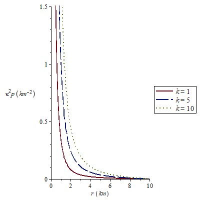
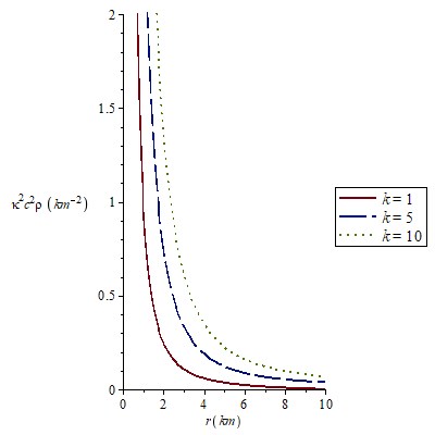
Using this constant, variation of the pressure and energy density as a function of the radial distance inside the star is given in Fig. 1. The interior of the star is considered as the specific fluid which has very high gravitational fields, electromagnetic fields and matter. Then the electromagnetic fields obey the modified Maxwell field equation in matter. The integral of the modified Maxwell equation (3) gives the charge in volume with radius in the star, (26). On the other hand, the Ricci scalar is zero at the exterior of the star and then, using (27), we can take the non-minimal function as and obtain the Maxwell field equation which leads to the the total charge at the exterior region. Here the displacement field inside of the star turns out to be the electric field outside. Setting by in eq. (26) the total charge of the star is found as
| (35) |
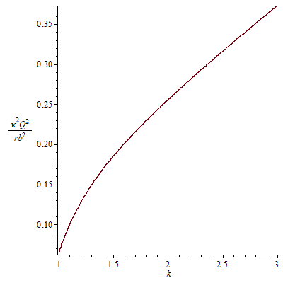
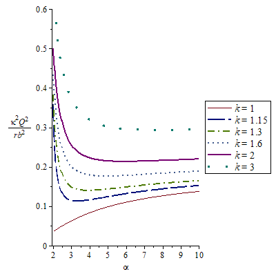
Then the outside electric field is given by . The total charge-boundary radius ratio obtained from (35) is plotted by Figure 2a dependent on the parameter for some different values.
The matter mass of the star can be found from the integral of the energy density
| (36) |
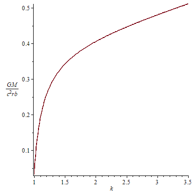
The figure of the matter mass is shown in Figure 2b for increasing and some different values. We see that the total charge and matter mass of the star increase with the increasing values.
When we compare the constant given by the equations (34) and (32), we find the following mass-charge relation for the model
| (37) |
By substituting the total charge (35) in (37), the total mass-radius ratio can be found in terms of the parameters and of the model
| (38) |
The gravitational redshift at the boundary is obtained from
| (39) |
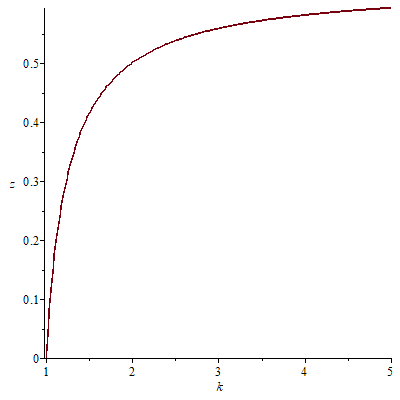
By taking the limit , the maximum redshift is found as same with in Sert2017 . The upper redshift bound is smaller than the Buchdahl bound and the bound given in Mak1 .
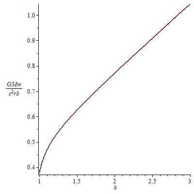
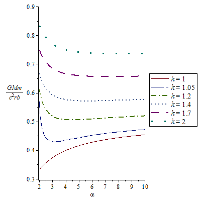
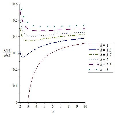
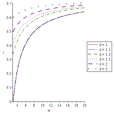
The mass-radius relation and the gravitational redshift-radius relation are shown in Figure 3a and 3b, respectively, depending on the parameter for some values. We see that as the k value increases, the mass and redshift increases.
To obtain an interval for the parameter we consider the energy density condition inside the star
| (40) |
At the center of the star the condition
| (41) |
gives . On the other hand, at the boundary the condition (40) turns out to be
| (42) |
The solution of the inequality (42) is
| (43) |
Then we can choose without loss of generality. The derivative of the pressure according to the energy density is calculated as
| (44) |
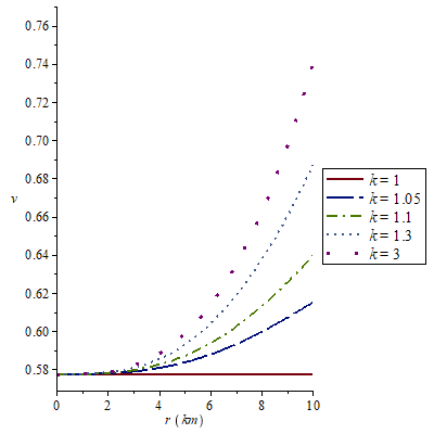
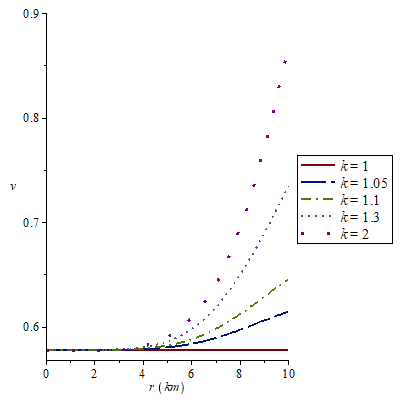
The phase speed of the sound waves in the star is defined by and the speed satisfies the causality condition for and values (see Fig. 6a for some values), where the speed of light . Thus each possible values of the parameters and in the modified model give a mass, charge-radius ratio and redshift .
IV.1 The simple model with
We consider the simple case setting by in the non-minimally coupled model (28)
| (45) |
Here we note that the non-minimal coupling function can be expanded as the binomial series in power of for .
| (46) |
The non-minimal model (45) accept the interior metric as a solution
| (47) |
together with the following electric field, pressure, energy density and electric charge from (22)-(26) inside of the star
| (48) | |||||
| (49) | |||||
| (50) | |||||
| (51) |
Then under the boundary and matching conditions the total charge, mass and gravitational redshift can be expressed by the followings
| (52) |
| (53) |
| (54) |
from (35)-(39). We note that the redshift has the upper bound for , which is smaller than the general redshift bound of the model which is . As the simple model with , we depict the related physical quantities in Fig 4-6. We give the corresponding values by taking the observed mass-radius ratios of some known stars and calculate the other quantities in Table 1. Here we note that each star have its own value and the each value can be determined by the observational mass and radius of the star.
| Star | (redshift) | |||
|---|---|---|---|---|
| EXO 1745-248 | Ozel2009 | 1.047 | 0.082 | 0.098 |
| 4U 1820-30 | Guver2010 | 1.084 | 0.095 | 0.156 |
| 4U1608-52 | Guver20102 | 1.098 | 0.099 | 0.174 |
| SAX J1748.9-2021 | Guver2013 | 1.135 | 0.110 | 0.217 |
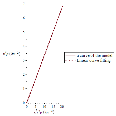
In order to obtain an approximate equation of state of the matter inside the star from equation (49) and (50), we fit the parametric curve with the equation
| (55) |
where we have used as a dimension-full constant. We note that if we obtain the radiation fluid case Sert2017 . The curve fitting is shown in Fig. 7. It is interesting to see that the fitting equation of state corresponds to the MIT bag model Witten ; Cheng which is given by . In this model the bag constant is related to the parameter as . If we set , we find , where we have used and . Then for and for . Additionally, we see that the parameter takes values approximately in the interval from the Table 1 for realistic compact stars. In the case , the non-minimal Einstein-Maxwell model with gives the gravitational mass using the radius . We see that this mass is less than the mass obtained for conformal symmetric charged stellar models in the minimal Einstein-Maxwell theory mak-harko-2004 . We note that the both models have the conformal symmetry and very similar interior metric solutions. Although this modified Einstein-Maxwell model has free parameters which can be set to be consistent with various compact star observations, the model in mak-harko-2004 determines a unique charged configuration of quark matter in terms of the Bag constant. Alternatively, the mass in our model increases to for , and for . That is, we can confine as which gives the Bag constant and consider is a free parameter, in order to describe compact stars.
V Conclusion
We have extended the solutions of the previous the non-minimally coupled theory Sert2017 to the case with under the symmetry of conformal motions. In the case without any assumption of the equation of state, we have acquired one more parameter in the solutions and the corresponding model. The pressure and energy density in the solutions are decreasing function with in the interior of the star.
By matching the interior solution with the exterior Reissner-Nordstrom solution and applying the zero pressure condition at the boundary radius of star , we determine some physical properties of the star such as the ratio of the total mass and charge to boundary radius and gravitational redshift depending on the parameters and .
We note that the total mass and charge increase with increasing values and we have not reach an upper bound for in the extended non-minimal model. But the increasing values give an upper bound for the gravitational redshift, , which is smaller than the more general restriction found in Mak1 for compact charged objects. It is interesting to note that each and value in this model (28) determines a different non-minimally coupled theory and each theory with the different parameters gives different mass-radius, charge-radius ratios and gravitational redshift configuration. We calculated values and the corresponding other quantities of the compact stars with the simple case via the some observed mass-radius values in Table 1. In this case, we also obtained the approximate equation of state (55) by fitting the curve of the model. By comparing the fitting equation of state with the MIT bag model for , we found the gravitational mass which is smaller than the mass obtained for conformal symmetric quark stars mak-harko-2004 in the Einstein-Maxwell theory. However the mass in our model increases as increases. The non-minimally coupled model has the arbitrary parameters and which can be set in order to be consistent with compact star observations. Even for , each value can describe a charged compact star.
References
- (1) D. Kramer, H. Stephani, M. MacCallum and E. Herlt, Exact solutions of Einstein’s field equations Cambridge: Cambridge University Press (1980).
- (2) M. S. R. Delgaty and K. Lake, Comput. Phys. Commun. 115, 395 (1998).
- (3) M. K. Mak, and T. Harko, Pramana, 65, 185, (2005).
- (4) M. K. Mak, and T. Harko, The European Physical Journal C, 73, 2585 (2013).
- (5) T. Harko, M. K. Mak, Astrophysics and Space Science, 361(9), 1-19 (2016).
- (6) R. Stettner, Ann. Phys. 80, 212 (1973).
- (7) A. Krasinski, Inhomogeneous cosmological models, Cambridge University Press (1997).
- (8) R. Sharma, S. Mukherjee and S.D. Maharaj, Gen. Relativ. Gravit. 33, 999 (2001).
- (9) M. K. Mak, and T. Harko, Int. J. Mod. Phys. D, 13, 149 (2004).
- (10) J. M. Overduin and P. S. Wesson, Physics Reports 402, 267 (2004).
- (11) H. Baer, K.-Y. Choi, J. E. Kim, and L. Roszkowski, Physics Reports 555, 1 (2015).
- (12) A. G. Riess et al., Astron. J. 116, 1009 (1998).
- (13) S. Perlmutter et al., Astrophys. J. 517, 565 (1999).
- (14) R. A. Knop et al., Astrophys. J. 598, 102 (2003).
- (15) R. Amanullah et al., Astrophys. J. 716, 712 (2010).
- (16) D. H. Weinberg, M. J. Mortonson, D. J. Eisenstein, C. Hirata, A. G. Riess, and E. Rozo, Physics Reports 530, 87 (2013).
- (17) D. J. Schwarz, C. J. Copi, D. Huterer and G. D. Starkman, Class. Quant. Grav. 33 184001 (2016).
- (18) B. Danila, T. Harko, F. S. N. Lobo, M. K. Mak, Phys. Rev. D 95, 044031 (2017).
- (19) T. Harko, F. S. N. Lobo, M. K. Mak, and S. V. Sushkov, Phys. Rev. D 88, 044032 (2013).
- (20) T. Dereli, Ö. Sert, Eur. Phys. J. C 71, 3, 1589 (2011).
- (21) Ö. Sert, Eur. Phys. J. Plus 127: 152 (2012).
- (22) Ö. Sert, Mod. Phys. Lett. A 28, 12, 1350049 (2013).
- (23) Ö. Sert and M. Adak, arXiv:1203.1531 [gr-qc].
- (24) M. Adak, Ö. Akarsu, T. Dereli, Ö. Sert, JCAP 11 026 (2017).
- (25) M. S. Turner and L. M. Widrow, Phys. Rev. D 37, 2743 (1988).
- (26) F. D. Mazzitelli and F. M. Spedalieri, Phys. Rev. D 52, 6694 (1995).
- (27) L. Campanelli, P. Cea, G. L. Fogli and L. Tedesco, Phys. Rev. D 77, 123002 (2008).
- (28) K. Bamba and S. D. Odintsov, JCAP (04), 024 (2008).
- (29) K. Bamba, S. Nojiri and S. D. Odintsov, JCAP, (10), 045, (2008).
- (30) T. Dereli, Ö. Sert, Mod. Phys. Lett. A 26, 20, 1487-1494 (2011).
- (31) A. R. Prasanna, Phys. Lett. 37A, 331 (1971).
- (32) G. W. Horndeski, J. Math. Phys. (N.Y.) 17, 1980 (1976).
- (33) F. Mueller-Hoissen, Class. Quant. Grav. 5, L35 (1988)
- (34) T. Dereli, G. Üçoluk, Class. Q. Grav. 7, 1109 (1990).
- (35) H.A. Buchdahl, J. Phys. A 12, 1037 (1979)
- (36) I.T. Drummond, S.J. Hathrell, Phys. Rev. D 22, 343 (1980)
- (37) K. E. Kunze, Phys. Rev. D 81, 043526 (2010) [arXiv:0911.1101 [astro-ph.CO]].
- (38) H.A. Buchdahl, Phys. Rev., 116 1027 (1959).
- (39) A. Baykal, T. Dereli, Phys.Rev. D92 6, 065018 (2015).
- (40) Ö. Sert, Journal of Mathematical Physics 57, 032501 (2016).
- (41) T. Dereli, Ö. Sert, Phys. Rev. D 83, 065005 (2011).
- (42) Ö. Sert, Eur. Phys. J. C 77 no.2, 97 (2017).
- (43) C. W. Misner and H. S. Zapolsky, Phys. Rev. Lett., 12, 635 (1964).
- (44) J. D. Bekenstein, Phys. Rev. D 4 2185 (1971).
- (45) J. L. Zhang, W. Y. Chau and T. Y. Deng, Astrophys. and Space Sc. 88 81, (1982).
- (46) F. de Felice, Y. Yu and Z. Fang, Mon. Not. R. Astron. Soc. 277 L17 (1995).
- (47) F. de Felice, S. M. Liu and Y. Q. Yu, Class. Quantum Grav. 16 2669 (1999).
- (48) Y. Q. Yu and S. M. Liu, Comm. Teor. Phys. 33 571 (2000).
- (49) P. Anninos and T. Rothman, Phys. Rev. D 65 024003 (2001).
- (50) S. Ray, A. L. Espindola, M. Malheiro, J. P. S. Lemos, V. T. Zanchin, Phys. Rev. D, 68:084004, (2003).
- (51) M. Malheiro, R. Picanço, S. Ray, J.P.S. Lemos, V.T. Zanchin, IJMP D, 13, 07, (2004).
- (52) R. Turolla, S. Zane and A. L. Watts, Reports on Progress in Physics, 78, 11, (2015) and references therein.
- (53) L. Herrera and J. Ponce de Leon, J. Math. Phys. 26, 2303, (1985).
- (54) L. Herrera and J. Ponce de Leon, J. Math. Phys. 26, 2018, (1985).
- (55) L. Herrera and J. Ponce de Leon, J. Math. Phys. 26, 778, (1985).
- (56) M. K. Mak, Peter N. Dobson Jr., T. Harko Europhys.Lett. 55 310-316 (2001).
- (57) F. Ozel, T. Guver, and D. Psaltis, APJ 693:1775–1779, (2009)
- (58) T. Guver, P. Wroblewski, L. Camarota, F. Ozel, APJ , 719, 1807, (2010)
- (59) T. Guver, F. Ozel, A. Cabrera-Lavers, and P. Wroblewski, APJ 712, 964, (2010)
- (60) T. Guver and F. Ozel, The Astrophysical Journal Letters, 765:L1 (4pp), (2013)
- (61) E. Witten, Phys. Rev D 30, 272, (1984).
- (62) K. S. Cheng, Z.G. Dai and T. Lu, Int. J. Mod. Phys. D 7, 139, (1998).