Simple analytical model of a thermal diode

Abstract

Recently there is a lot of attention given to manipulation of heat by constructing thermal devices such as thermal diodes, transistors and logic gates. Many of the models proposed have an asymmetry which leads to the desired effect. Presence of non-linear interactions among the particles is also essential. But, such models lack analytical understanding. Here we propose a simple, analytically solvable model of a thermal diode. Our model consists of classical spins in contact with multiple heat baths and constant external magnetic fields. Interestingly the magnetic field is the only parameter required to get the effect of heat rectification.

1 Introduction

Recently heat transport in microscopic systems has attracted a lot of attention. These studies mainly involve studying heat transport in terms of verification of Fourier’s law at molecular scale using detailed microscopic models A. Dhar ; Lepri et.al ; Saito ; B. Hu et.al ; Chang2008 et.al ; Yang2010 et.al . Looking at the working of small scale devices, such as engines, thermal/electronic pumps or analogous thermal rectification devices like diode, transistors, logic gates etc. is also of interest Lo et.al ; Saira et.al ; Baowin2006a ; BaowinRMP2012 ; Baowin2004 ; Liang et.al ; Li et.al ; Wang2007 & Li ; Marathe07 . These effects have been studied in classical as well as quantum mechanical systems, and have also been realized experimentally Chang2006 et.al ; Kim et.al ; Wu2007 & Li ; Wu2008 & Li ; Yang2008 et.al ; Yang2009 et.al ; Hu2009 et.al ; Gonzalez et.al ; Jiang et.al ; ChenNatComm17 . Thermal diodes, transistors and logic gates have been modeled using classical harmonic oscillator chains with non-linear interactions and acted upon by different on-site potentials Baowin2006a ; BaowinRMP2012 ; Wang2007 & Li ; Baowin2004 . The mismatch of the on-site potentials and phonon modes as well as the non-linear interactions play crucial role in such models to get the desired effect of heat rectification. These thermal devices were also modeled using classical spins BLeePRE11 ; Bagchi13 ; Bagchi15 . In these models anisotropic parameter and mismatch of the spin flipping rate at the interface of two spin networks in contact with different heat baths are the underlying factors for the rectification of heat current.

Due to non-linear interactions among the constituents analytical understanding becomes difficult. However, many interesting analytical attempts have been made to understand basic principles behind heat rectification, for example in harmonic chains with quartic potential PereiraPRE10 as well as studying sufficiency conditions for thermal rectification PereiraPRE11 . In mass-graded harmonic chains with temperature dependent effective potential PereiraPRE17 and also in quantum harmonic chains PereiraPLet10 . Here we propose a simple model of a thermal diode which is in principle analytically tractable. Our model consists of coupled classical spins, with nearest neighbor interactions. One segment of the spins is in contact with a thermal reservoir at temperature $T_{L}$ and the other with a thermal reservoir at temperature $T_{R}$. Spins are also acted upon by external constant magnetic fields $h_{L}$ and $h_{R}$ respectively. Interestingly the externally applied magnetic field is the only control parameter for our thermal device.

The paper is organized as follows. We first describe the model of the thermal diode then we provide the results for this model. We conclude with a discussion of our results.

2 Model

The system we consider is divided into left and right segments. The left (suffix $(L)$) segment has $N_{L}$ number of Ising spins and right (suffix $R$) segment has $N_{R}$ number of Ising spins as shown in Fig. 1. The Hamiltonian of the system is given by:

$$\mathcal{H}=-J\sum\limits_{\langle i,j\rangle}\sigma_{i}~{}\sigma_{j}-\mu h_{L}\sum\limits_{i=1}^{N_{L}}\sigma_{i}-\mu h_{R}\sum\limits_{i=1}^{N_{R}}\sigma_{i},$$ (1)

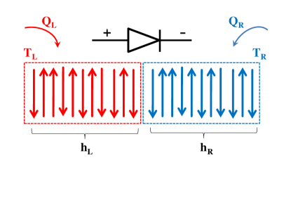
Figure 1: Schematic diagram of thermal diode with classical Ising spins. The red (left) segment consisting $N_{L}$ spins subjected to an external magnetic field $h_{L}$ and in contact with heat bath at temperature $T_{L}$. The $N_{R}$ spins in blue (right) segment are in contact with heat bath at temperature $T_{R}$ acted upon by a constant external magnetic field $h_{R}$.

where, $J$ is the interaction energy between the spins, $\mu$ is the magnetic moment of spins, $h_{L}$ and $h_{R}$ are the external magnetic fields. Each spin can take two values $\sigma_{i}$=$\pm 1$ and $\langle i,j\rangle$ represents nearest neighbor interaction. Since the spins are in thermal contact with the temperature reservoirs, the flipping of the spins is a stochastic process and the master equation governing this stochastic evolution of probabilities is:

$$\frac{\partial\hat{P}(\left\{\sigma\right\},t)}{\partial t}=\hat{\mathcal{T}}\hat{P}(\left\{\sigma\right\},t),$$ (2)

where $\hat{\mathcal{T}}$ is the Transition Matrix, $\hat{P}(\left\{\sigma\right\},t)$ is the spin distribution function, where $\left\{\sigma\right\}$ represents spin configuration at time $t$, such that $\hat{P}(\{\sigma\},t)=\hat{P}(\sigma_{1},\sigma_{2},...,t)$.

The dynamics of the spins with respective heat baths is modeled by a Metropolis algorithm generalized to accommodate multiple heat reservoirs. The choice of algorithm is generic and our results qualitatively do not depend on particular form of the flipping probabilities, for example Glauber dynamics. The elements in the transition matrix $\hat{\mathcal{T}}$ give the rates of transition from one configuration to other. If a spin flips then the rate of this flip is given by:

$$r^{L,R}_{\sigma_{i}}=~{}min(1,~{}e^{-\beta_{L,R}\Delta{E_{L,R}}}),$$ (3)

where, $\beta_{L,R}=1/k_{B}T_{L,R}$ is chosen depending on which segment the spin belongs to and $\Delta{E_{L,R}}=2J(\sigma_{i}\sigma_{i-1}+\sigma_{i}\sigma_{i+1})+2\mu h_{L,R}\sigma_{i}$ is the difference in the energy after and before the flip. In our analysis we have chosen the Boltzmann constant $k_{B}$ and $\mu$ to be unity. For larger system sizes one may also resort to Monte Carlo simulations where a spin is chosen at random and is flipped with probabilities given above. Here the flipping probability is nothing but the rate $r^{L,R}_{\sigma_{i}}$ multiplied by the the time step $dt$. In each $dt$ time step only a single spin flip is allowed.

This modified Metropolis algorithm for multiple heat baths allow us to write general expression for the heat currents in the system. $\dot{Q}_{L,R}$ are the heats coming from the left and the right baths respectively. In our model, heat coming into the system from the reservoirs is taken to be positive. The expression for the heat currents are:

$$\dot{Q}_{L,R}=\sum_{\left\{\sigma\right\}}r^{L,R}_{\sigma_{i}}\Delta{E_{L,R}}\hat{P}(\left\{\sigma\right\}).$$ (4)

In principle for any system size, given the transition matrix $\hat{\mathcal{T}}$, Eq. (2) can be solved analytically in the steady state. Since in the steady state $\frac{\partial\hat{P}}{\partial t}=0$, thus $\hat{P}(\left\{\sigma\right\})$ is nothing but the eigenvector of the matrix $\hat{\mathcal{T}}$ corresponding to the eigenvalue zero vankampen . Once the steady state probabilities $\hat{P}(\left\{\sigma\right\})$ are obtained, both heat currents can also be evaluated. In the next section we describe the working of the thermal diode using definitions above.

3 Thermal Diode

We now describe working of our model as a thermal diode. Here we give a particular example for a small system consisting of just two Ising spins, first one in contact with a bath at temperature $T_{L}$ and second with $T_{R}$. We fix $h_{R}=0$ without loss of generality. With these parameters and Eq. (3) we can determine the matrix elements of $\hat{\mathcal{T}}$. Using steady state probabilities P($\sigma_{1},\sigma_{2}$) along with the normalization condition $\sum\limits_{\sigma_{1},\sigma_{2}}P(\sigma_{1},\sigma_{2})=1$, heat currents defined in Eq. (4) turn out to be:

$$\dot{Q}_{L} =~{}2(J+\mu h_{L})~{}\left[e^{-2\beta_{L}(J+\mu h_{L})}P(1,1)-P(-1,1)\right]$$

$$+2(\mu h_{L}-J)\left[e^{-2\beta_{L}(\mu h_{L}-J)}P(1,-1)-P(-1,-1)\right],$$

$$\dot{Q}_{R} =~{}2J~{}\left[e^{-2\beta_{R}J}P(1,1)-P(1,-1)-P(-1,1)+e^{-2\beta_{R}J}P(-1,-1)\right].$$

where,

$$P(1,1) =~{}e^{2\beta_{L}\mu h_{L}+\beta_{R}J}~{}[e^{\beta_{L}(J-\mu h_{L})}\cosh(\beta_{L}(\mu h_{L}-J)+\beta_{R}J)$$

$$+\cosh(\beta_{R}J)]/\mathcal{D},$$

$$P(1,-1) =~{}e^{2\beta_{L}\mu h_{L}-\beta_{R}J}~{}[e^{2\beta_{R}J-\beta_{L}(\mu h_{L}+J)}\cosh(\beta_{L}(\mu h_{L}+J)-\beta_{R}J)$$

$$+\cosh(\beta_{R}J)]/\mathcal{D},$$

$$P(-1,1) =~{}[e^{-\beta_{L}(J+\mu h_{L})}\cosh(\beta_{L}(\mu h_{L}-J))$$

$$+~{}\cosh(2(\beta_{L}-\beta_{R})J)]/\mathcal{D},$$

$$P(-1,-1) =~{}e^{\beta_{R}J}~{}[e^{\beta_{L}(J-\mu h_{L})}\cosh(\beta_{L}(\mu h_{L}+J)-\beta_{R}J)$$

$$+~{}\cosh((2\beta_{L}-\beta_{R})J)]/\mathcal{D},$$

$$\mathcal{D} =~{}2\cosh(\beta_{R}J)[e^{2\beta_{L}\mu h_{L}}\cosh(\beta_{R}J)+e^{\beta_{R}J}\cosh(2\beta_{L}\mu h_{L})]$$

$$+~{}2\left[e^{\beta_{R}J}+\cosh(\beta_{R}J)\right]\cosh((2\beta_{L}-\beta_{R})J),$$

Eq. (LABEL:qlqr) is the steady state expression for $\dot{Q}_{L}$ and $\dot{Q}_{R}$ in terms of $P(\sigma_{1},\sigma_{2})$. After some simplification we get:

$$\dot{Q}_{L} =~{}4~{}J\sinh(2(\beta_{R}-\beta_{L})J)/\mathcal{D},$$ (6)

$$\dot{Q}_{R} =~{}4~{}J\sinh(2(\beta_{L}-\beta_{R})J)/\mathcal{D}.$$

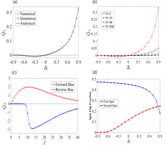
Figure 2: The parameters used are $J=1$, $h_{L}=10$, $T_{0}=10$, and $h_{R}=0$. $(a)$ Heat current versus the temperature bias for the system with two Ising spins. The plot consists the results from numerical techniques, simulations and analytical solution of the Master Equation. $(b)$ Heat current versus the temperature bias for different system sizes. $(c)$ Heat current versus the interaction term $J$. Here $h_{L}=10$ and $h_{R}=0$. For forward biased case $T_{L}=19$ and $T_{R}=1$, and for the reverse biased case $T_{L}=1$ and $T_{R}=19$. $(d)$ Spin flip fraction versus the temperature bias for the system with two Ising spins. The plot shows the fraction of first spin and the second spin flips in a simulation. Zero line is just a guide for the eyes.

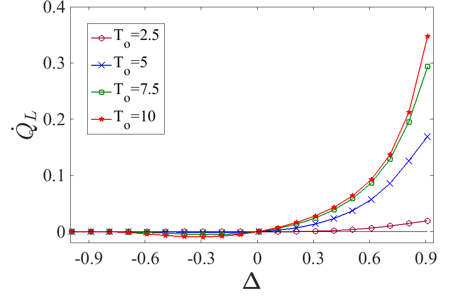
Figure 3: Plot of heat current versus $\Delta$ for different reference temperatures $T_{0}$ for a two spin system with $J=1$, $h_{L}=10$, $h_{R}=0$.

The heat currents $\dot{Q}_{L}$ and $\dot{Q}_{R}$ are related by just a sign change. Also the heat currents vanish when $T_{L}=T_{R}$, as expected.

To study the characteristic of working of a diode, we define, $T_{L}=T_{0}(1+\Delta)$ and $T_{R}=T_{0}(1-\Delta)$ where $\Delta$ is relative temperature bias and $T_{0}$ is the reference temperature. Negative values of $\Delta$ correspond to reverse biased operation $(T_{R}>T_{L})$ and positive to forward biased operation $(T_{L}>T_{R})$. We plot the heat current $\dot{Q}_{L}$ as a function of $\Delta$. In Fig. 2$(a)$ the graph shows comparison of results obtained from direct simulations, numerical solution of the Master equation and exact solution Eq. (6). Data from all the three calculations match perfectly. We can see that in the reverse biased case thermal current is extremely low as compared to the forward biased case. In Fig. 2$(b)$ we show the results for systems with different system sizes. The graphs again depict that our model works as a thermal diode even for larger systems. It is well known that the asymmetry in the system causes rectification. In the model considered here, the unequal magnetic fields on the two segments provide this asymmetry, making it work as a heat rectifying device.

From Fig. 2$(c)$ it can be observed that the heat rectification occurs only when $J$ is less than $\mu h_{L}$. This happens because in the forward biased mode $T_{L}>T_{R}$ and though the spin experiences magnetic field $h_{L}$, thermal energy dominates and the left spin flips, resulting in large current from left to right bath. However in the reverse biased case magnetic field $h_{L}$ dominates over the interaction energy $J$ and since $T_{L}<T_{R}$, thermal energy is not enough to flip the spin. Hence, the current reduces drastically. To quantify this, in Fig. 2$(d)$ we plot the fraction of number of flips of the first and second spin as a function of $\Delta$. In the reverse biased mode number of spin flips of the first spin are negligibly small as compared to the second spin, resulting in small current. But as we go from reverse biased mode to forward biased mode they slowly become comparable to each other and a large current flows in the system. We can also obtain asymptotic values of $\dot{Q}_{L,R}$ when $\Delta\rightarrow\pm 1$. Notice that as $\Delta\rightarrow 1$, $T_{L}\rightarrow 2T_{0}$ and $T_{R}\rightarrow 0$ hence terms with $\beta_{R}$ dominate conversely when $\Delta\rightarrow-1$, $T_{L}\rightarrow 0$ and $T_{R}\rightarrow 2T_{0}$ and terms with $\beta_{L}$ dominate. From the Eqs. (LABEL:qlqr) and (6) some simple algebra results into:

$$\dot{Q}_{L}\rightarrow\begin{cases}4J/A&,\Delta\rightarrow 1\\ \\ {\large\frac{-2J\exp\left(-2\beta_{R}J\right)}{\left(B\exp\left(2\beta_{L}(\mu h_{L}-J)\right)~{}+~{}C\right)}\ }&,\Delta\rightarrow-1,\end{cases}$$ (7)

where:

$$A = 2\exp(2\beta_{L}(\mu h_{L}+J))+\exp(2\beta_{L}(J-\mu h_{L}))+3,$$

$$B = \cosh(\beta_{R}J)\left(2\cosh(\beta_{R}J)+\exp(\beta_{R}J)\right),$$

$$C = 1+\exp(-\beta_{R}J)\cosh(\beta_{R}J).$$

It is straight forward to check that in the forward biased mode current approaches a finite positive value and in reverse biased mode, only when $\mu h_{L}>J$, current approaches zero from below as seen from Fig. 2$(a)$, $(c)$. For particular values of the parameters namely $\Delta=-0.9$ and $T_{0}=10$, we have $T_{L}=1.0$ and $T_{R}=19.0$, with $h_{L}=10.0$ and $h_{R}=0$, we get $\dot{Q}_{L}\sim 10^{-10}$ and for $\Delta=0.9$ it is $\sim 0.35$. Fig. 3 shows the diode operation for different reference temperatures $T_{0}$.

Finally we study the rectification efficiency of our device. For this we define the rectification factor $R$:

$$R=\left(\frac{\dot{Q}_{L}-\dot{Q}_{R}}{\dot{Q}_{R}}\ \right)\times 100\%,$$ (8)

where $\dot{Q}_{L}$ is measured when the device is in the forward biased mode and $\dot{Q}_{R}$ when it is in the reverse biased mode. Recent study has shown that this factor can be made independent of the system size with a ballistic spacer placed between two anharmonic chains CasatiArxv17 . We plot rectification factor for our model for different parameters in Fig. 4. We can clearly see that for almost all parameters $R$ can be made very large.

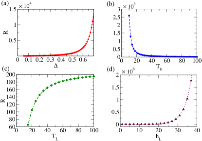
Figure 4: Plot of rectification factor $R$ versus different model parameters. Parameters wherever applicable are $J=1$, $h_{L}=10$. $(a)$ $R$ versus $\Delta$ here $T_{0}=10$. $(b)$ $R$ versus $T_{0}$ with $\Delta=\pm 0.6$ in forward/reverse biased mode. Here $h_{L}$ may also be increased with $T_{0}$, so that $R$ does not decrease. $(c)$ $R$ versus $T_{L}$ where $T_{R}=10$ is fixed and $T_{L}$ varied. $(d)$ $R$ versus $h_{L}$ parameters used are $T_{0}=10$, $\Delta=\pm 0.5$ in forward/reverse biased mode.

In heat conduction problems involving linear harmonic oscillators, heat current turns out to be proportional to the temperature difference $(T_{L}-T_{R})$ A. Dhar ; Marathe07 , for such a system rectification is not possible unless the interactions are non-linear BAgarwalla . In our model however the current does not depend linearly on the temperature difference as seen from Eq. (6). Non-linearity is introduced through the flipping rates Eq. (3). Even then the analytical expressions for the heat currents are obtained, this distinguishes our model from the earlier studied models.

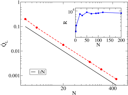
Figure 5: Plot of heat current $\dot{Q}_{L}$ in the forward biased mode $(\Delta=0.8)$ as a function of system size $N$. One can clearly see the $1/N$ dependence of heat current on system size. Inset rectification factor $R$ defined in the text as a function of system size for $|\Delta|=0.8$. Interestingly $R$ goes to a constant value as $N$ increases. Other parameters are $J=1$, $h_{L}=10$, $T_{0}=10$.

4 Conclusion

To conclude, we have studied a simple model of a thermal diode composed of classical Ising spins connected to multiple heat reservoirs and are in the presence of constant external magnetic fields. Ising spins undergo stochastic dynamics governed by usual Metropolis algorithm, modified to take care of multiple heat baths. Interestingly external magnetic field is the only parameter which makes the models work as a thermal rectifier. Although our model has a non-linearity inbuilt in the transition rates, we are able to get analytical results for any system size. Here we note that, if say $N_{L}$ number of spins are in contact with reservoir at temperature $T_{L}$ and $N_{R}$ with temperature $T_{R}$, the current in large system size just scales as $\sim 1/N$ if $N_{L}=N_{R}=N$ $($Fig. 5$)$. On the other hand rectification factor $R$ seems to become constant as system size increases $($inset of Fig. 5$)$, which is an interesting effect. A similar two-level quantum mechanical model was studied in BLeePRB09 where the heat rectification was observed. Our study thus ascertains that even in classical discrete systems such a phenomenon is possible. Study on effect of long range interactions in our model will be interesting. Such interactions seem to increase the rectification efficiency AvilaPRE13 . However, analytical calculation of heat currents with long range interactions may not be possible. Extension of our model to other thermal devices namely transistors, logic gates is currently underway. We believe experimental realization of such a model is possible in nanoscale solid state devices.

Acknowledgments
Authors thank the IIT Delhi HPC facility for computational resources. Authors also thank Arnab Saha for careful reading of the manuscript.

Author contribution statement
SauK and SacK performed simulations and analytical calculations. RM devised the study, performed simulations and analytical calculations. SauK, SacK and RM wrote the paper.

References

- (1) B. Hu, B. Li, and H. Zhao, Phys. Rev. E 57, 2992 (1998).
- (2) S.Lepri, R. Livi, and A. Politi, Phys. Rep. 377, 1 (2003).
- (3) C. W. Chang, D. Okawa, H. Garcia, A. Majumdar, and A. Zettl, Phys. Rev. Lett. 101, 075903 (2008).
- (4) A. Dhar, Adv. Phys. 57, 457 (2008).
- (5) K. Saito, and A. Dhar, Phys. Rev. Lett. 104, 040601 (2010).
- (6) N. Yang, G. Zhang, and B. Li, Nano Today 5, 85 (2010).
- (7) B. Li, L. Wang, and G. Casati, Phys. Rev. Lett. 93, 184301 (2004).
- (8) B. Li, L. Wang, and G. Casati, Appl. Phys. Lett. 88, 143501 (2006)
- (9) O.P. Saira, M. Meschke, F. Giazotto, A. M. Savin, M. Möttönen, and J. P. Pekola, Phys. Rev. Lett. 99, 027203 (2007)
- (10) L. Wang and B. Li, Phys. Rev. Lett. 99, 177208 (2007).
- (11) W. Lo, L. Wang, and B. Li, J. Phys. Soc. Jpn. 77, 054402 (2008)
- (12) R. Marathe, A. M. Jayannavar, and A. Dhar, Phys. Rev. E 75, 030103(R) (2007).
- (13) B. Liang, B. Yuan, and J.-c. Cheng, Phys. Rev. Lett. 103, 104301 (2009).
- (14) X. F. Li, X. Ni, L. Feng, M.-H. Lu, C. He, and Y.-F. Chen, Phys. Rev. Lett. 106, 084301 (2011).
- (15) N Li, J Ren, L Wang, G Zhang, P Hänggi, B Li, Rev. Mod. Phys. 84(3), 1045 (2012).
- (16) P. Kim, L. Shi, A. Majumdar, and P. L. McEuen, Phys. Rev. Lett. 87, 215502 (2001)
- (17) C. W. Chang, D. Okawa, A. Majumdar, and A. Zettl, Science 314, 1121 (2006).
- (18) G. Wu, and B. Li, Phys. Rev. B 76, 085424 (2007).
- (19) Wu, G., and B. Li, J. Phys. Condens. Matter 20, 175211 (2008).
- (20) N. Yang, G. Zhang, and B. Li, Appl. Phys. Lett. 93, 243111 (2008).
- (21) N. Yang, G. Zhang, and B. Li, Appl. Phys. Lett. 95, 033107 (2009).
- (22) J. Hu, X. Ruan, and Y. P. Chen, Nano Lett. 9, 2730 (2009).
- (23) E. Gonzalez Noya, D. Srivastava, and M. Menon, Phys. Rev. B 79, 115432 (2009).
- (24) J. Jiang, J. Wang, and B. Li, Euro. Phys. Lett. 89, 46005 (2010).
- (25) H. Wang, S. Hu, K. Takahashi, X. Zhang, H. Takamatsu, and J. Chen, Nature Comm. 8, 15843 (2017).
- (26) L. Wang and B. Li, Phys. Rev. E 83, 061128 (2011).
- (27) D. Bagchi, J. Phy.: Condensed Matter 25 (49), 496006 (2013).
- (28) D. Bagchi, J. Stat. Mech.: Theory and Experiment P02015 (2015).
- (29) E. Pereira, Phys. Rev. E 82, 040101 (R) (2010).
- (30) E. Pereira, Phys. Rev. E 83, 031106 (2011).
- (31) E. Pereira, Phys. Rev. E 96, 012114 (2017).
- (32) E. Pereira, Phys. Lett. A 374, 1933 (2010).
- (33) N. G. van Kampen, Stochastic Processes in Physics and Chemistry (North Holland 2007).
- (34) Liu Sha, B. K. Agarwalla, B. Li, and J. -S. Wang, Phys. Rev. E 87, 022122 (2013).
- (35) S. Chen, D. Donadio, G. Benenti and G. Casati, arXiv:1712.03373.
- (36) E. Pereira and R. R. Avila, Phys. Rev. E, 888, 032139 (2013).
- (37) Y. Yan, C-Q. Wu, and B. Li, Phys. Rev. B 79, 014207 (2009).