Drag-Based Ensemble Model (DBEM) for Coronal Mass Ejection Propagation

Abstract

The drag-based model (DBM) for heliospheric propagation of coronal mass ejections (CMEs) is a widely used analytical model which can predict CME arrival time and speed at a given heliospheric location. It is based on the assumption that the propagation of CMEs in interplanetary space is solely under the influence of magnetohydrodynamical drag, where CME propagation is determined based on CME initial properties as well as the properties of the ambient solar wind. We present an upgraded version, covering ensemble modelling to produce a distribution of possible ICME arrival times and speeds, the drag-based ensemble model (DBEM). Multiple runs using uncertainty ranges for the input values can be performed in almost real-time, within a few minutes. This allows us to define the most likely ICME arrival times and speeds, quantify prediction uncertainties and determine forecast confidence. The performance of the DBEM is evaluated and compared to that of ensemble WSA-ENLIL+Cone model (ENLIL) using the same sample of events. It is found that the mean error is $ME=-9.7$ hours, mean absolute error $MAE=14.3$ hours and root mean square error $RMSE=16.7$ hours, which is somewhat higher than, but comparable to ENLIL errors ($ME=-6.1$ hours, $MAE=12.8$ hours and $RMSE=14.4$ hours). Overall, DBEM and ENLIL show a similar performance. Furthermore, we find that in both models fast CMEs are predicted to arrive earlier than observed, most probably owing to the physical limitations of models, but possibly also related to an overestimation of the CME initial speed for fast CMEs.

1 Introduction

As coronal mass ejections (CMEs) are dominating space weather effects, including potentially harmful impacts for Earth, the forecasting of CMEs is one of the major challenges for space weather forecast. Therefore, in recent years many CME and their associated shock propagation models have been developed by research groups around the globe and space weather forecast centers regularly implement some of these propagation models to alert about a possible arrival of potentially threatening CMEs (e.g. Space Weather Prediction Center of the National Oceanic and Atmospheric Administration, SWPC/NOAA, in USA, Met Office in UK or Solar Influences Data Analysis Center, SIDC, in Belgium).

The propagation models differ based on the input, approach, assumptions and complexity (for overview see e.g.  Zhao and Dryer, 2014, and references therein) and vary from simple empirical models (e.g.  Gopalswamy et al., 2001), neural network models (e.g.  Sudar et al., 2016), analytical drag-based models with different geometries (e.g.  Vršnak et al., 2014; Rollett et al., 2016), various kinematic shock propagation models (e.g.  Dryer et al., 2001; Zhao et al., 2016; Takahashi and Shibata, 2017) to complex numerical 3D MHD models such as the H3DMHD model (Wu et al., 2011) or WSA-ENLIL+Cone model (Odstrcil et al., 2004). Despite these differences, in general most of the models show a surprisingly comparable performance, where the prediction errors are mostly found within the 24-hour interval and the mean absolute error is $\sim 10$ hours (e.g.  Gopalswamy et al., 2001; Li et al., 2008; Vršnak et al., 2014; Mays et al., 2015; Sudar et al., 2016; Wold et al., 2017).

The drag-based models are based on the concept of MHD drag, which, unlike the kinetic drag effect in a fluid, is presumed to be caused primarily by the emission of MHD waves in the collisionless solar wind environment and acts to adjust the CME speed to the ambient solar wind (Cargill et al., 1996). The concept of drag relies on the observational fact that slow CMEs accelerate whereas fast CMEs decelerate (e.g.  Sheeley et al., 1999; Gopalswamy et al., 2000) and is supported by numerous studies (e.g.  Vršnak and Žic, 2007; Temmer et al., 2011; Liu et al., 2013; Hess and Zhang, 2014; Sachdeva et al., 2015, and references therein). Vršnak and Žic (2007) proposed that the equation describing the aerodynamic drag can be utilised to establish a simple kinematical drag-based model (DBM) for CME propagation, which was since developed by implementing the cone geometry of a CME and performing parametric analysis to empirically determine the drag parameter $\gamma$ (Vršnak et al., 2013, 2014; Žic et al., 2015). The DBM is available at Hvar Observatory website as an online tool, it is one of the European Space Agency (ESA) space situational awareness (SSA) products, is one of the models available at the Community Coordinated Modeling Center (CCMC), and is incorporated into the automatic COMESEP system (Crosby et al., 2012; Dumbović et al., 2017). The performance of DBM was shown to be comparable to that of other propagation models (Vršnak et al., 2014) and was furthermore found to agree well with WSA-ENLIL+Cone model, which is one of the most extensively used CME propagation models in space weather operations world-wide.

The resemblance in the performance of very different propagation models indicates that the major drawback in more accurately forecasting CME arrival times and impact speeds is the lack of reliable observation-based input. In order to take into account the errors and uncertainties in the CME measurements that are used as model input and for quantifying the resulting uncertainties in the model predictions, ensemble forecasting is widely used. Recently, Mays et al. (2015) used an ensemble modelling approach to evaluate the sensitivity of WSA-ENLIL+Cone model (hereafter ENLIL) simulations to initial CME parameters and provide a probabilistic forecasting of CME arrival time. Ensemble modelling takes into account the variability of observation-based model input by making an ensemble, i.e. sets of $n$ CME observations to calculate a distribution of predictions and forecast the confidence in the likelihood of the CME arrival. We use the ensemble approach in DBM and present the newly developed DBEM. The model is evaluated on the same data set as Mays et al. (2015) to be compared to ENLIL ensemble results.

2 Data and method

DBEM is based on DBM with assumed cone geometry for the CME, where the leading edge is initially a semicircle, spanning over the full angular width of the CME and flattens as it evolves in time (described in Žic et al., 2015). The model assumes a constant solar wind speed, $w$, and drag parameter, $\gamma$, which is in general valid for distances beyond $R>15\mathrm{R_{SUN}}$, where the CME moves in an isotropic solar wind spreading out at a constant speed and the fall-off of the ambient density is at the same rate as the CME expansion (see Vršnak et al., 2013; Žic et al., 2015). As this assumption is clearly not valid for CME-CME interaction events (Temmer et al., 2012), we do not consider such interaction events in our study. We note that the constant $w$ and $\gamma$ assumption can be generally valid even for CMEs moving in high speed streams, assuming they encounter high speed streams relatively close to the Sun.

The input parameters derived from observations and used as input for the DBEM are the CME speed, halfwidth, and propagation direction (longitude) defined at a certain distance/time from the Sun. Since this is a 2D model that operates in the ecliptic plane DBEM does not use CME latitude as an input. The solar wind speed (the radial component in the ecliptic plane) and the drag parameter, $\gamma$, complete the input values. In a first step, for a single CME, we use an ensemble of $n$ measurements of the same CME as Mays et al. (2015) (see Section 2.1). Next, the variability of DBM parameters (solar wind speed, $w$ and drag parameter, $\gamma$) is taken into account, where $m$ synthetic values of both $w$ and $\gamma$ are produced (see Section 2.2). These synthetic values are combined with an ensemble of $n$ CME measurements, to give a final ensemble of $n\cdot m^{2}$ members as an input, which, after $n\cdot m^{2}$ runs, produces a distribution of $n\cdot m^{2}$ calculated CME transit times and arrival speeds.

2.1 CME initial parameters

We use the sample compiled and analysed by Mays et al. (2015), which consists of 35 CMEs and associated interplanetary CMEs (ICMEs, if detected at Earth) in the time period January 2013 to July 2014. All CME measurements and simulation summary results are available at https://iswa.ccmc.gsfc.nasa.gov/ENSEMBLE/. The CME initial parameters are determined using the Stereoscopic CME Analysis Tool (StereoCAT) developed by CCMC. StereoCAT tracks specific CME features, based on triangulation of transient CME features manually identified using two different coronagraph fields-of-view. From this the 3D speed and position is derived for a CME as well as its (projected) width. To gather an ensemble of measurements, the CME leading edge height was measured for two different times in each coronagraph image for two different coronagraph viewpoints and then the procedure was repeated $k$ times to obtain an ensemble of $n=k^{2}$ CME measurements (for details see Mays et al., 2015). Each ensemble member has a specific set of initial CME parameters - speed, width, longitude and latitude. Given that a typical run of the whole ensemble using ENLIL simulations is 80–130 min (depending on the computing power), for each event an optimal spread of input parameters was selected ($n=12,16,24,36,48$). It should be noted that the input is more suitable for the 3D ENLIL WSA+cone model, which uses both longitude and latitude as positional parameters and 3D velocity as input speed, whereas for DBEM the radial component of velocity in the ecliptic plane would be a more suitable input.

We refine the sample compiled by Mays et al. (2015) excluding events with CME-CME interaction and events where in situ arrival times could not be determined exactly and unambiguously. The resulting sample consists of 25 CMEs and for each event we use as ensemble model input the derived speed, halfwidth, longitude, and start time. The start time corresponds to the starting distance, which is restrained by the ENLIL inner boundary corresponding to $R=21.5\mathrm{R_{SUN}}$ and is also suitable for DBM due to the assumption of constant $w$ and $\gamma$ and furthermore because after that distance the drag is the dominant force governing the propagation of ICMEs for a large subset of CMEs (Sachdeva et al., 2015, 2017).

2.2 Solar wind speed and drag parameter $\gamma$

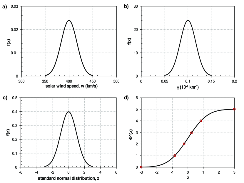
Figure 1: Normal distributions for a) $w=(350\pm 50)$ $\mathrm{km~{}s}^{-1}$and b) $\gamma=(0.1\pm 0.05)$ $\cdot 10^{-7}~{}\mathrm{km}^{-1}$; c) standard normal distribution obtained with substitution $z=(x-\mu)/\sigma$; d) cumulative standard normal distribution normalised so that it is defined on an interval [0,$m-1$], where $m=6$ is the number of synthetic values in this example ($\Phi_{i}^{*}(z)=0,1,2,3,4,5$ are outlined in red).

As input values for the solar wind speed, $w$, and drag parameter, $\gamma$, we do not use measured values, but empirical values derived in previous studies by Vršnak et al. (2013, 2014). Therefore, to include their uncertainty in DBEM similarly to the uncertainty of the CME input (CME ensembles), synthetic values are needed. Synthetic values of $w$ and $\gamma$ for a specific event can be produced assuming that the real measurements of these parameters follow a normal distribution fully defined by the following expression:

$$x=\bar{x}\pm\Delta x\,,$$ (1)

where $\bar{x}=\mu$ is the mean of the normal distribution and $\Delta x=3\cdot\sigma$ defines a range where 99,7% measurements are found ($\sigma$ is the standard deviation). The normal distribution for a random variable $x$, $f(x)$, is defined for a specific $\mu$ and $\sigma$, where $w$ and $\gamma$ are treated as random variables described by a normal distribution. In Figures 1a and 1b examples of normal distributions are shown for $w=(350\pm 50)$ $\mathrm{km~{}s}^{-1}$and $\gamma=(0.1\pm 0.05)$ $\cdot 10^{-7}~{}\mathrm{km}^{-1}$, respectively. Based on our assumption, these are the distributions we would obtain by making real measurements of $w$ and $\gamma$, where their real values are found in the intervals $w=(350\pm 50)$ $\mathrm{km~{}s}^{-1}$and $\gamma=(0.1\pm 0.05)$ $\cdot 10^{-7}~{}\mathrm{km}^{-1}$, respectively.

Using the substitution $z=(x-\mu)/\sigma$, a corresponding standard normal distribution (SND), $f(z)$, is obtained, which is normalised with respect to the original distribution so that $\mu=0$ and $\sigma=1$ (shown in Figure 1c). The cumulative SND, which is the probability that $z$ will take a value less than or equal to some $z_{0}$ (i.e. gives the area under $f(z)$ from $-\infty$ to $z_{0}$), can be written as:

$$\Phi(z)=\frac{1}{2}\bigg{(}1+\operatorname{erf}{(\frac{z}{\sqrt{2}})}\bigg{)}\,,$$ (2)

where the $\operatorname{erf}{(z)}$ is the Gauss error function defined as:

$$\operatorname{erf}{(z)}=\frac{2}{\sqrt{\pi}}\int_{0}^{z_{0}}e^{-z^{2}}dz\,.$$ (3)

$\Phi(z)$ is a continuous function defined on an interval [0,1]. However, if multiplied with a normalisation factor $m-1$, where $m$ is the number of synthetic values we wish to produce, we obtain a new continuous function $\Phi^{*}(z)$ defined on an interval [0,$m-1$], which can be used to obtain $m$ different values of $z$:

$$z_{i}=-\sqrt{2}\cdot\operatorname{erf}^{-1}{\bigg{(}1-2\frac{\Phi_{i}^{*}(z)}{m-1}\bigg{)}},\qquad\Phi_{i}^{*}(z)=0,1,2,...,m-2,m-1\,.$$ (4)

This is graphically represented in Figure 1d on an example where $m=6$. Each $z_{i}$ corresponds to a certain $x_{i}$ based on the substitution $z_{i}=(x_{i}-\mu)/\sigma$. Therefore, for a given number $m$ and a parameter defined according to Equation 1, $m$ synthetic values of the parameter can be produced based on Equation 4. An example is given in Figures 2a and 2b, where $m=25$ synthetic values are shown against the normal distributions for $w=(350\pm 50)$ $\mathrm{km~{}s}^{-1}$and $\gamma=(0.1\pm 0.05)$ $\cdot 10^{-7}~{}\mathrm{km}^{-1}$, respectively.

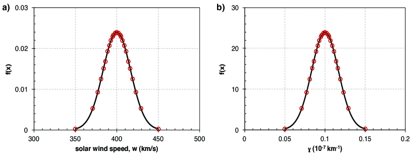
Figure 2: Normal distributions for a) $w=(350\pm 50)$ $\mathrm{km~{}s}^{-1}$and b) $\gamma=(0.1\pm 0.05)$ $\cdot 10^{-7}~{}\mathrm{km}^{-1}$and corresponding synthetic values (red circles).

Based on Figure 2 it is obvious that the synthetic values will reflect the normal distribution closer if larger $m$ is chosen. However, very large $m$ will increase the number of runs and consequently computing time. Therefore, the optimum $m$ needs to be determined. For that purpose, we randomly selected a CME from our list which has a total of 48 ensemble members (2014 February 12). We then randomly selected 3, 5, 8, 12, 24, and 36 ensemble members to simulate respective ensemble sizes of the same CME (different ensemble sizes are denoted with $n$). For each of the ensembles we made model runs using different number of synthetic values $m=3,5,7,10,15,20,30,50,100$ and derived distributions of transit times, $TT$(h), and arrival speeds, $v$($\mathrm{km~{}s}^{-1}$), from which we calculate the median and $95\%$ confidence interval. The model runs include both the variability of the CME input ($n$) and the variability of the model parameters ($m$). In order to observe how the values of distribution median and $95\%$ confidence interval change with $n$ and $m$, we normalised for each $n$ the difference of the $m$-th median to the median corresponding to a value of 100 in the following way:

$$dX(n,m)=\frac{|X(n,m)-X(n,100)|}{X(n,100)}\,,$$ (5)

where $X(n,m)$ is the median of $TT$ and $v$ for CME transit time and arrival speed, respectively. We applied the same equation to $95\%$ confidence interval as well, where for each $n$ the difference of the $m$-th $95\%$ confidence interval is normalised to the $95\%$ confidence interval corresponding to $m=100$ according to Equation 5 with $X(n,m)$ being $TT_{\mathrm{range}}$ and $v_{\mathrm{range}}$ for CME transit time and arrival speed, respectively. This is shown in Figure 3 where it can be seen that the variability of the median for both arrival speed and transit time is quite small ($<1\%$ for arrival speed, $<3\%$ for transit time) and decreases with both $n$ and $m$. The variability of the $95\%$ confidence interval is much larger (can go up to $30\%$ for transit time and even $60\%$ for arrival speed), but also decreases quickly with increasing $n$ and $m$. Both the median and the $95\%$ confidence interval converge quite fast towards the value corresponding to $m=100$. At $m=15$ the variability of the median is already below $0.5\%$ for all CME ensemble sizes $n$ for both $TT$ and $v$, whereas the variability of the $95\%$ confidence interval is below $5\%$ for $TT$ and around $10\%$ for $v$. We note that the typical prediction errors of the CME transit time are $\sim 10$ hours (as described in Section 1), thus a $5\%$ variation in a confidence interval would correspond to less than $\sim 1$ hour and a $0.5\%$ variation of the median would be of the order of magnitude of $\sim 1$ minute. Therefore, as an optimal value we choose $m=15$. For an ensemble of $n=48$ CME inputs, with this optimal value of $m=15$ synthetic $w$ and $\gamma$ values the total number of model runs is $n\cdot m^{2}=10800$, resulting in a computational time of several minutes on an average PC.

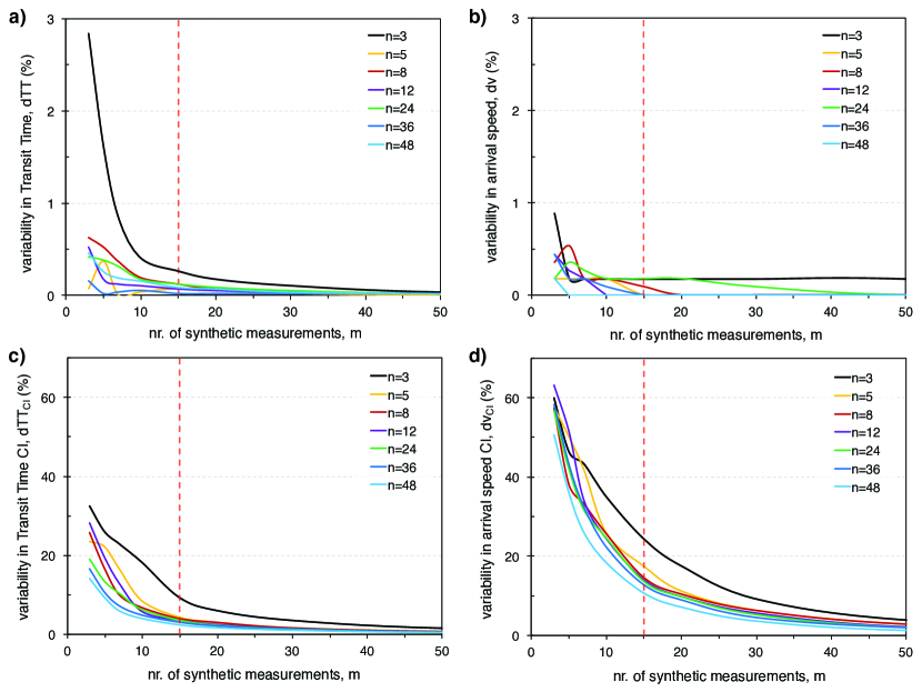
Figure 3: The variability of the distribution median for a) CME transit time and b) arrival speed, and of the $95\%$ confidence interval for c) CME transit time and d) arrival speed depending on the number of CME ensemble members, $n$ and number of solar wind speed and $\gamma$ parameter synthetic values, $m$. The variabilities are normalised to values corresponding to $m=100$ (for each CME ensemble separately). The red dashed line marks the optimal value $m=15$ (for details see main text).

For simplicity we use the same value of mean solar wind speed and $\gamma$ parameter for all events in the sample. Due to the weak solar activity throughout the last solar cycle, which was reflected on the solar wind and interplanetary magnetic field (e.g.  McComas et al., 2013), we use $w=(350\pm 50)$ $\mathrm{km~{}s}^{-1}$. DBM tracks the leading edge of the ICME ejecta, whereas ENLIL tracks the shock front. However, it was shown that there is in general a good agreement between the two with a convenient selection of the $\gamma$ parameter ($\gamma=0.1$$\cdot 10^{-7}~{}\mathrm{km}^{-1}$, see Vršnak et al., 2014). Therefore, in order to estimate shock arrival with DBEM we select $\gamma=(0.1\pm 0.05)$ $\cdot 10^{-7}~{}\mathrm{km}^{-1}$. With these values of $w$ and $\gamma$ we determine $m=15$ synthetic values of $w$ and $\gamma$ with the procedure described above. It should be noted that the simplification of using average solar wind conditions results in less realistic solar wind background than the one used by ENLIL.

3 Results and Discussion

For each ensemble member, i.e. individual run, DBEM calculates whether or not the CME will hit or miss the Earth. The corresponding condition can be written as $\omega\geq|\phi|$, where $\omega$ is the CME halfwidth and $\phi$ is the CME source position longitude. For the whole ensemble DBEM calculates the probability of the arrival as $p=n_{\mathrm{hits}}/n_{\mathrm{tot}}$, where $n_{\mathrm{hits}}$ is the number of ensemble members that are calculated to hit Earth and $n_{\mathrm{tot}}$ is the total number of all ensemble members. The probability of arrival for a CME is displayed as a pie chart, as shown in the upper right panel of Figure 4 where DBEM results for the example CME 2013 August 30 are given. As can be seen in Figure 4 the probability of arrival for this event, as calculated by DBEM is 0.92 (91.7%, red part of the pie chart). The CME input for this event consists of 48 ensemble members with start time range 05:59 UT to 06:30 UT, CME speed range $810-1012$ $\mathrm{km~{}s}^{-1}$, longitude range E55${}^{\circ}-$E35^∘, and halfwidth range 41${}^{\circ}-63^{\circ}$. This is supplemented with 15 synthetic values of solar wind speed in the range $300-400$ $\mathrm{km~{}s}^{-1}$and 15 synthetic values of the drag parameter $\gamma$ in the range $0.05-0.15$ $\cdot 10^{-7}~{}\mathrm{km}^{-1}$. Therefore, the size of the whole ensemble for this example is 10800, i.e. the results are based on 10800 DBM runs. A table of the first eight ensemble members (input lines) is given in the top left panel as a quicklook visualisation of the input.

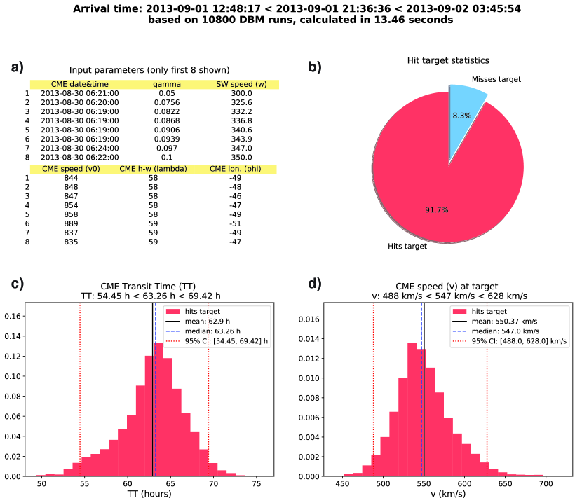
Figure 4: DBEM results for the 2013 August 30 CME: a) a quicklook table of the (partial) input; b) a pie chart with the probability of arrival; c) the distribution of the CME transit time; d) the distribution of the arrival speed. Distributions of the CME transit time and arrival speed are calculated only for ensemble members that hit Earth and are given with the corresponding distribution parameters (mean, median and $95\%$ confidence interval). The median (most likely) arrival time and the $95\%$ confidence interval are given on top with a basic performance record (number of runs and calculation time).

The bottom panels in Figure 4 show transit time, $TT$, and arrival speed, $v$, distributions, calculated only based on the runs for ensemble members calculated to hit Earth (the red part of the pie chart). The expected range is given by the $95\%$ confidence interval. The most likely arrival date and time and corresponding range are given on the top of Figure 4 and are also calculated only based on ensemble members predicted to hit Earth. The output also provides a quick performance record - the number of runs and the computing time. The example event shown in Figure 4 was run on an average PC. Depending on the number of CPUs and their speed, the current DBEM version can make thousand (on single thread/CPU) or more runs per second and can run the whole ensemble in several minutes, which is very fast compared to ENLIL runtime ($>1$ hour on a high-performance machine, see Section 2.1). We perform the DBEM forecast evaluation for a set of 25 events, and when possible, compare the outcome to that of ENLIL. Forecast evaluation is based on DBEM and ENLIL calculations of $TT$, DBEM calculation of $v$, and in situ observations of $TT$ and $v$ presented in Table 1 (for additional information on the median values of the CME input we refer the reader to Table 1 of Mays et al., 2015). We use the peak value of the in situ speed to be consistent in all events, due to the fact that sometimes only shock/sheath is encountered, sometimes only ICME magnetic structure and sometimes both.

CME	ICME	Observed	Observed	DBEM									ENLIL
start	arrival	$TT$	$v$	$p_{i}$	$TT$	$\Delta T_{\mathrm{err}}$	$TT_{\mathrm{min}}$	$TT_{\mathrm{max}}$	$v$	$\Delta v_{\mathrm{err}}$	$v_{\mathrm{min}}$	$v_{\mathrm{max}}$	$p_{i}$	$TT$	$\Delta T_{\mathrm{err}}$	$TT_{\mathrm{min}}$	$TT_{\mathrm{max}}$
date	date & time	(h)	$\mathrm{km~{}s}^{-1}$	(%)	(h)	(h)	(h)	(h)	$\mathrm{km~{}s}^{-1}$	$\mathrm{km~{}s}^{-1}$	$\mathrm{km~{}s}^{-1}$	$\mathrm{km~{}s}^{-1}$	(%)	(h)	(h)	(h)	(h)
2013
04/11	04/13 22:13	62.8	520	100	48.2	-14.6	40.4	56.3	653	133	556	807	100	46.8	-16	41.4	52.9
06/21	06/23 03:51	48.7	720	97.9	34.8	-13.9	28.5	42	841	121	676	1137	97.9	33.9	-14.8	30.3	39.6
08/02	–	–	–	0	–	CR	–	–	–	–	–	–	0	–	CR	–	–
08/07	–	–	–	100	74	FA	–	–	–	–	–	–	100	–	FA	–	–
08/30	09/02 01:56	71.1	510	91.7	63.3	-7.8	54.5	69.4	547	37	488	628	95.8	53.7	-17.4	48.3	58.3
09/19	–	–	–	0	–	CR	–	–	–	–	–	–	0	–	CR	–	–
09/29	10/02 01:15	52.6	630	100	50.8	-1.8	39.7	62.4	627	-3	526	793	100	55.5	2.9	44.7	64.6
10/06	10/08 19:40	53	650	100	58.3	5.3	47.5	64.6	569	-81	503	681	91.7	79.5	26.5	69.7	89.6
10/22	–	–	–	100	58	FA	–	–	–	–	–	–	95.7	–	FA	–	–
2014
01/07	01/09 19:39	49.3	480	100	26.3	-23	19.8	33.9	1019	539	772	1474	100	29.9	-19.4	23	39.1
01/30	02/02 23:20	78.9	470	87.5	59	-19.9	44.6	78.1	563	93	459	721	54.2	65.7	-13.2	53.4	77.6
01/31	–	–	–	100	68.7	FA	–	–	–	–	–	–	100	–	FA	–	–
02/12	02/15 12:46	79.1	450	100	58.2	-20.9	49.7	72.2	562	112	475	663	100	66.1	-13	57.4	79.3
02/18	02/20 02:42	49.3	690	75	59.5	10.2	30.3	86.2	558	-132	424	926	80.6	63.1	13.8	34.4	80.8
02/19	02/23 06:09	86.2	510	100	53.1	-33.1	43.5	62.2	604	94	518	743	88.9	68.4	-17.8	55.8	81.6
02/25	02/27 15:50	62.7	500	54.2	38.2	-24.5	29.5	55.2	763	263	580	1038	83.3	45.1	-17.6	33.8	65.8
03/23	03/25 19:10	63.4	520	43.8	72	8.6	58.1	85.5	497	-23	431	592	79.2	69.2	5.8	56.6	81
03/23	–	–	–	8.3	114.4	CR	–	–	–	–	–	–	0	–	CR	–	–
03/29	–	–	–	50	75.2	FA	–	–	–	–	–	–	5.6	–	CR	–	–
04/02	04/05 10:00	68.4	500	31.2	43.5	-24.9	37	50.4	710	210	598	891	87.5	53.4	-15	43.3	59.7
04/18	04/20 10:20	45.2	700	100	37.8	-7.4	31.7	43.8	780	80	644	1010	100	40	-5.2	36	46.1
06/04	06/07 16:12	72.4	610	88.9	79	6.6	66	110.8	460	-150	354	539	61.1	77.1	4.7	69	83.9
06/10	–	–	–	2.8	61.4	CR	–	–	–	–	–	–	5.6	–	CR	–	–
06/19	06/22 18:28	73.3	410	100	79.7	6.4	68	92.3	460	50	403	530	100	71	-2.3	65.6	78.6
06/30	–	–	–	0	–	CR	–	–	–	–	–	–	0	–	CR	–	–

Table 1: Observed and calculated transit times for the 25 CMEs under study using DBEM and ENLIL. $p_{i}$ is the probability of arrival, $TT$ is the transit time, and $v$ is the arrival speed. $\Delta T_{\mathrm{err}}=TT_{\mathrm{predicted}}-TT_{\mathrm{observed}}$ and $\Delta v_{\mathrm{err}}=v_{\mathrm{predicted}}-v_{\mathrm{observed}}$ are prediction errors, whereas $TT_{\mathrm{min}}$/$TT_{\mathrm{max}}$ and $v_{\mathrm{min}}$/$v_{\mathrm{max}}$ define the arrival spread (the 95% confidence interval) for $TT$, and $v$, respectively. CR and FA denote correct rejection and false alarm, respectively (for explanation see main text).

The probability of arrival, $p_{i}$ is binned into a categorical yes/no forecast using a $p_{i}<15\%$ criterion for correct rejection, same as was used in Mays et al. (2015). Thus a 2x2 contingency table for a binary event can be constructed and used to perform forecast evaluation (see e.g.  Jolliffe and Stephenson, 2003), where CME arrival is regarded as an event, and the event forecast as well as the event observation can have two outcomes, yes or no. There are four possible combinations of forecast and observation outcomes: a “hit” where the event was forecasted to hit Earth and observed, a “miss” where the event was not forecasted to hit Earth but was observed, a “false alarm” where the event was forecasted to hit Earth but was not observed and a “correct rejection”, where the event was neither forecasted nor observed. Following the procedure by Mays et al. (2015), if $p_{i}<15\%$ and there were no in situ signatures, the event (CME arrival) is considered as a “correct rejection”; if $p_{i}>15\%$ and there were no in situ signatures, the event is considered as a “false alarm”; if $p_{i}>15\%$ and there are in situ signatures, the event is considered as a “hit”; and finally, if $p_{i}<15\%$ and there are in situ signatures, the event is considered as a “miss”.

		DBEM	ENLIL
a) contingency table results
Number of hits	$a$	16	16
Number of misses	$c$	0	0
Number of false alarms	$b$	4	3
Number of correct rejections	$d$	5	6
Number of events	$N=a+b+d$	25	25
b) evaluation measures
Correct rejection rate	$d/(b+d)$	55.6%	66.7%
False alarm rate	$b/(b+d)$	44.4%	33.3%
Correct alarm ratio	$a/(a+b)$	80.0%	84.2%
False alarm ratio	$b/(a+b)$	20.0%	15.8%
Brier score	$BS$ (see Equation 6 )	0.17	0.18
c) prediction errors for $TT$ (h)
mean error ($ME$)		-9.7	-6.1
mean absolute error ($MAE$)		14.3	12.8
root mean square error ($RMSE$)		16.7	14.4
d) prediction errors for $v$ ($\mathrm{km~{}s}^{-1}$)
mean error ($ME$)		84	–
mean absolute error ($MAE$)		133	–
root mean square error ($RMSE$)		181	–

Table 2: Contingency table results, evaluation measures and prediction errors for DBEM and ENLIL (calculated based on the sample presented in Table 1).

The number of hits, misses, false alarms and correct rejections for our sample is given in Table 2a for DBEM and ENLIL, and the outcome using different evaluation measures is given in Table 2b. Compared to ENLIL, DBEM has out of 25 events one false alarm more and one correct rejection less than ENLIL, which results in a somewhat lower performance. In the final row of Table 2b a Brier score ($BS$) is given, which quantifies the probability forecast errors:

$$BS=\frac{1}{N}\sum_{i=1}^{N}(p_{i}-o_{i})^{2}\,,$$ (6)

where $N$ is the total number of events, $p_{i}$ is the forecast probability that event $i$ will occur, and $o_{i}$ takes value 0 if event $i$ did not occur and 1 if the event $i$ did occur. For perfect forecast $BS=0$ and we can see that both DBEM and ENLIL are not too far away from this value.

In Table 2c transit time errors are given for DBEM and ENLIL, calculated for “hit” events. It can be seen that DBEM has somewhat larger errors than ENLIL. One of the reasons is that the CME input used is more suitable for ENLIL than DBEM. Optimal CME input for ENLIL is a full 3D information of the CME as given in the sample (3D velocity, longitude and latitude) while for DBEM optimal input would be the radial velocity in the ecliptic plane. Possibly an even more important issue is the ambient solar wind state. ENLIL used a more realistic solar wind background, whereas DBEM assumed average solar wind conditions for all CMEs ($w\sim 350$ $\mathrm{km~{}s}^{-1}$, $\gamma\sim 0.1$ $\cdot 10^{-7}~{}\mathrm{km}^{-1}$) not taking into account possible event–to–event variability (e.g. propagation through high speed streams). Another aspect which was not considered is a possible preconditioning effect, when an earlier CME “clears the path” effectively reducing $\gamma$ (Liu et al., 2014), which can be even ten times lower than the present average value in extreme cases (Temmer and Nitta, 2015). Therefore, it is reasonable to assume that DBEM would perform better if a more realistic solar wind background is considered and if the radial speed in the ecliptic plane was used. Nevertheless, overall these errors are still comparable to CME arrival time prediction errors reported in other studies (see e.g.  Li et al., 2008; Vršnak et al., 2014; Mays et al., 2015; Sudar et al., 2016; Wold et al., 2017, and references therein).

Next we test the performance of DBEM using the so called reliability diagram, which shows how well the predicted probabilities of an event correspond to their observed frequencies, i.e. how well the model predicts the probability of arrival (see e.g.  Jolliffe and Stephenson, 2003). In order to obtain the reliability diagram the events were binned according to their forecasted probability of arrival into 5 “bins”: $0\%$, [$0-33\%$], [$33-66\%$], [$66-100\%$], and $100\%$. For each bin an observed relative frequency was calculated as $\sum_{i=1}^{N_{o}}{O_{i}}/N_{o}$, where $N_{o}$ is the number of events corresponding to the bin and $O_{i}$ takes a value 0 if event $i$ did not occur and 100 if the event $i$ did occur. The line of perfect reliability is the identity line, i.e. in a perfectly reliable forecast the forecast probability equals the observed relative frequency. The reliability diagram based on the selected sample for DBEM and ENLIL is shown in Figure 5a, where the number of events used in each calculation is shown next to each point. Although some points are calculated based on only 2 events observed, the diagram can reflect some general aspects of the DBEM and ENLIL forecast reliability. It can be seen that for the $100\%$ bin both DBEM and ENLIL overforecast, i.e. predict higher probability of CME arrival than is observed, in agreement with a notable value of the false alarm rate in Table 2. For $0\%$ bin the point lies on the line of perfect reliability for both ENLIL and DBEM, however it should be noted that this is related to the fact that there are no missing alarms for neither model. With the intermediate bins one should be careful with drawing conclusions due to small number of calculations in some points, but at a descriptive level it would seem that both models slightly underforecast (ENLIL being closer to the line of perfect reliability). Similar conclusions were drawn for ENLIL by Mays et al. (2015) with an extended sample and slightly different selection of bins (see Figure 9a in Mays et al., 2015).

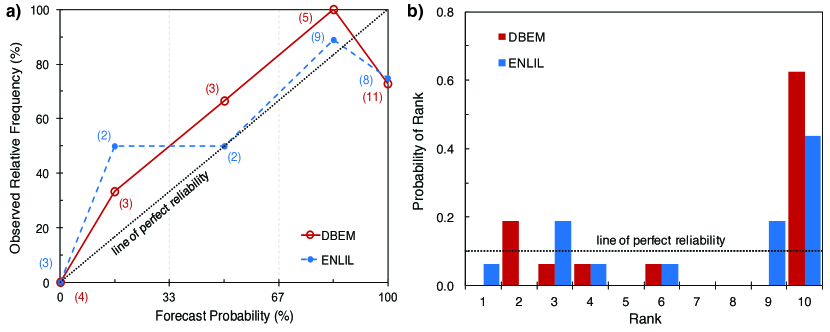
Figure 5: a) Reliability diagram of the forecast probability of CME arrival for the whole sample of 25 events; b) Rank histogram for the 16 hits.

In Figure 5b a rank diagram (also known as the “Talagrand” diagram) is shown, which reflects how well the ensemble spread of the forecast represents the true variability of the observations, i.e. whether observations statistically belong to the forecasted distributions (see e.g.  Hamill, 2001, and references therein). The rank diagram is constructed by sorting the $n$ ensemble members and the observation for each event from earliest to latest arrival time and “counting” at which place we find the observation with respect to other ensemble members (denoted as “rank”). For a perfect forecast, where we can statistically regard the observation as another member of the ensemble the observation is equally likely to occur in each of the $n+1$ possible “ranks”. Due to the fact that not all events have same ensemble sizes and moreover, that ensemble sizes for DBEM are drastically increased by introducing the $w$ and $\gamma$ synthetic values, we follow the same procedure as Mays et al. (2015) and normalise the rank number to $n=9$ (in total 10 possible ranks). The “perfect reliability” line in Figure 5b represents an ideally flat distribution where each rank has the same probability (i.e. 1.6 events per rank).

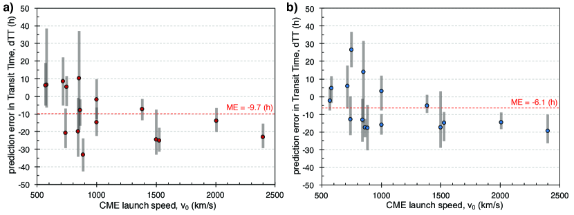
Figure 6: CME arrival time prediction error plotted against the CME input speed for a) DBEM and b) ENLIL. Error bars represent the spread in the ensemble forecasts.

It can be seen, that the rank diagram for both ENLIL and DBEM deviates from the perfect reliability. For both models the rank diagram shows an U-shape which indicates under-variability of the ensemble and an asymmetrical shape, which indicates a bias. For both DBEM and ENLIL the possible bias is towards under-forecasting, i.e. predicting smaller transit times than observed (also visible from the negative mean error presented in Table 2b). This is also supported by the fact that in only 38% of events the observed $TT$ can be found within the DBEM prediction spread, whereas for ENLIL this percentage is somewhat higher (50%). The possible reason for this bias could be related to fast CMEs. Mays et al. (2015) found that in their (extended) sample ENLIL generally predicted fast CMEs to arrive earlier than they were observed. To confirm this assumption, CME arrival time prediction errors are plotted against the CME input speed in Figure 6. An almost consistent negative prediction error can be seen for both DBEM and ENLIL for fast CMEs above $\sim$1000 $\mathrm{km~{}s}^{-1}$, cf. Figure 8a by Mays et al. (2015). This indicates that fast CMEs are indeed predicted to arrive earlier than observed for both ENLIL and DBEM, and results in a negative mean error and a bias towards under-forecasting. This might be related to model limitations, since they do not take into account all relevant physical processes. Liu et al. (2013, 2016) found that fast CMEs (with speed above 1000 $\mathrm{km~{}s}^{-1}$) differ from slower CMEs by a rapid deceleration process, which is not taken into account by DBEM and ENLIL. This would result in earlier predictions and overestimated arrival speed. Indeed, as seen in Table 2d and Figure 8a, DBEM has a tendency to overforecast the arrival speed for fast CMEs. It should also be noted that the role of CME-driven shocks is not considered in the drag based model (Reiner et al., 2003; Liu et al., 2013, 2016). DBM considers the physics of the magnetic structure of CMEs, not their related shocks, and it only estimates the shock arrival time using empirically obtained proxy value of $\gamma$ (Vršnak et al., 2014). Another possible reason could be an overestimation of the CME initial speed for fast CMEs, as suggested by Mays et al. (2015). Although DBEM and ENLIL use a range of CME initial speed as input, a large systematic overestimation of CME speed in the ensemble (e.g. due to limited number of measurement points in fast events) could lead to the observed underforecast of transit times and overforecast of arrival speed.

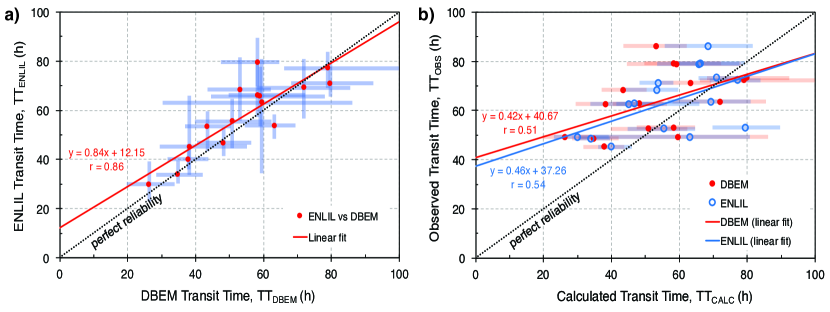
Figure 7: a) ENLIL-calculated vs. DBEM-calculated transit time; b) Observed vs. calculated transit time for ENLIL (blue) and DBEM (red). Solid lines represent the linear best fits, with corresponding equations and correlation coefficients $r$. The dotted line represents the identity line (perfect match). Error bars represent the spread in the ensemble forecasts.

Finally, we examine the correlation between observed and calculated transit times. In Figure 7a ENLIL-calculated transit time is plotted as a function of DBEM-calculated transit time. It can be seen that there is some scatter and the linear best fit somewhat deviates from the identity line, but in general there is a good agreement between ENLIL-calculated and DBEM-calculated transit times, similar to the results obtained for non-probabilistic ENLIL and DBM by Vršnak et al. (2014). In Figure 7b, the observed transit time is plotted as a function of calculated transit time for ENLIL (blue) and DBEM (red). It can be seen that both for ENLIL and DBEM the linear best fit substantially deviates from the identity line. This is seen in the linear best fit coefficients, where the slope is much smaller than 1 and the intercept much larger than 0. Furthermore it can be seen that for higher calculated transit times the scatter is around the identity (perfect) line, whereas for smaller calculated transit times the scatter is above the identity line, which is related to the fact that fast CMEs are predicted to arrive earlier than observed. In Figure 8b, the observed arrival speed is plotted as a function of calculated arrival speed for DBEM. Similar to transit times, it can be seen that the linear best fit substantially deviates from the identity line, related to the overforecast of the arrival speed (for smaller values of calculated arrival speeds the scatter is around the identity line, whereas for larger values of calculated arrival speeds the scatter is below the identity line). We note that there seems to be an outlier with calculated $v=1019$ $\mathrm{km~{}s}^{-1}$. When the outlier is removed the slope of the best linear fit obtains a value of 0.36 and thus improves towards the identity line, and the correlation coefficient increases to $r=0.42$. We note that the outlier seems not to appear in the transit time calculation (Figure 7b), but only in the calculation of arrival speed (Figure 8b).

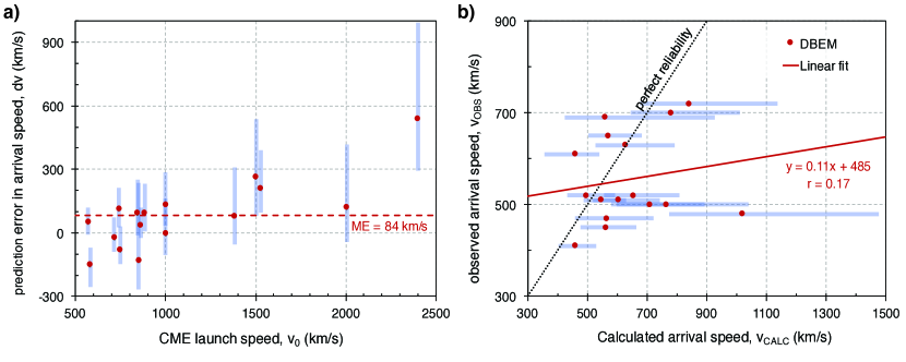
Figure 8: a) CME arrival speed prediction error for DBEM plotted against the CME input speed; b) Observed vs. calculated arrival speed for DBEM. Solid line represents the linear best fit, with corresponding equation and correlation coefficient $r$. The dotted line represents the identity line (perfect match). Error bars represent the spread in the ensemble forecasts.

4 Summary and Conclusion

We present a probabilistic approach in the drag-based CME propagation modelling, the drag-based ensemble model (DBEM), which is available as an online tool at Hvar Observatory website, and as one of the European Space Agency (ESA) space situational awareness (SSA) products. An ensemble of $n$ members is used as a CME input, where the variation in model parameters is also taken into account by constructing the synthetic values of solar wind speed, $w$, and drag parameter, $\gamma$. $m$ synthetic values of $w$ and $\gamma$ are constructed under the assumption that the measurements are behaving as random variables and follow a normal distribution. The model input thus consists of $n\cdot m^{2}$ ensemble members, where $n$ is restricted by the observations and optimal $m$ was found as a compromise between the convergence of the output distribution and the computing time. The outputs are probability of arrival and distributions of CME transit times and arrival speeds, where the median is taken as the most likely value and the range is defined with $95\%$ confidence interval. Therefore, DBEM is able to provide probabilities of CME arrival at a specific target together with uncertainties in the arrival time and speed.

We evaluated the performance of the new DBEM model on a refined sample taken from the study by Mays et al. (2015), where it can also be compared to the performance of ENLIL. Depending on the number of CPUs and their speed, DBEM can perform thousand (on a single CPU) or more runs per second and is several orders of magnitude faster than ENLIL, which is its main advantage. Comparison between DBEM and ENLIL revealed that ENLIL performs slightly better than DBEM, most probably owing to the more realistic background solar wind conditions and a more suitable CME input (3D velocity). Despite small differences, the performance of the two models is similar and comparable to a “standard” CME prediction error in transit time of $\sim 10$ hours. We find that for this particular sample in both models fast CMEs are predicted to arrive earlier than observed, related to model limitations and possibly also to the overestimation of the CME initial speed for fast CMEs. Since both models show similarly good, as well as bad results, additional actions should probably be taken in order to improve the overall CME arrival forecast. A possible improvement might be to use different propagation models for different solar activity conditions. This approach, as well as the ensemble forecasting, would be analogous to the methods used in meteorology, where different models are used for different conditions since there is not a single model that is capable of forecasting the weather for all types of regions. In line with this view, the “CME Scoreboard” website can serve as the platform to compare different models simulating/forecasting a variety of CME events occurring in real-time. Anyone is invited to submit their estimate of the arrival time of a recently observed CME in real-time to the CME Scoreboard. Therefore, it is suitable for model validation under real-time conditions and in addition provides an ensemble mean CME arrival time forecast from a variety of models and methods. The possible benefits from this type of approach are yet to be evaluated in future studies.

References

- Cargill et al. [1996] P. J. Cargill, J. Chen, D. S. Spicer, and S. T. Zalesak. Magnetohydrodynamic simulations of the motion of magnetic flux tubes through a magnetized plasma. J. Geophys. Res., 101:4855–4870, March 1996. 10.1029/95JA03769.
- Crosby et al. [2012] N. B. Crosby, A. Veronig, E. Robbrecht, B. Vršnak, S. Vennerstrom, O. Malandraki, S. Dalla, L. Rodriguez, N. Srivastava, M. Hesse, D. Odstrcil, and COMESEP Consortium. Forecasting the space weather impact: The COMESEP project. In Space weather: The space radiation environment: 11th annual international astrophysics conference, volume 1500 of Amer. Inst. Phys. CP, pages 159–164, 2012. http://dx.doi.org/10.1063/1.4768760.
- Dryer et al. [2001] M. Dryer, C. D. Fry, W. Sun, C. Deehr, Z. Smith, S.-I. Akasofu, and M. D. Andrews. Prediction in Real Time of the 2000 July 14 Heliospheric Shock Wave and its Companions During the ‘Bastille’ Epoch∗. Sol. Phys., 204:265–284, December 2001. 10.1023/A:1014200719867.
- Dumbović et al. [2017] M. Dumbović, N. Srivastava, Y. K. Rao, B. Vršnak, A. Devos, and L. Rodriguez. Validation of the CME Geomagnetic Forecast Alerts Under the COMESEP Alert System. Sol. Phys., 292:96, August 2017. 10.1007/s11207-017-1120-5.
- Gopalswamy et al. [2000] N. Gopalswamy, A. Lara, R. P. Lepping, M. L. Kaiser, D. Berdichevsky, and O. C. St. Cyr. Interplanetary acceleration of coronal mass ejections. Geophys. Res. Lett., 27:145–148, January 2000. 10.1029/1999GL003639.
- Gopalswamy et al. [2001] N. Gopalswamy, A. Lara, S. Yashiro, M. L. Kaiser, and R. A. Howard. Predicting the 1-AU arrival times of coronal mass ejections. J. Geophys. Res., 106:29207–29218, December 2001. 10.1029/2001JA000177.
- Hamill [2001] T. M. Hamill. Interpretation of Rank Histograms for Verifying Ensemble Forecasts. Monthly Weather Review, 129(3):550–560, 2001. 10.1175/1520-0493(2001)129¡0550:IORHFV¿2.0.CO;2.
- Hess and Zhang [2014] P. Hess and J. Zhang. Stereoscopic Study of the Kinematic Evolution of a Coronal Mass Ejection and Its Driven Shock from the Sun to the Earth and the Prediction of Their Arrival Times. Astrophys. J., 792:49, September 2014. 10.1088/0004-637X/792/1/49.
- Jolliffe and Stephenson [2003] I. T. Jolliffe and D. B. Stephenson. Forecast Verification: A Practioner’s Guide in Atmospheric Science. John Wiley & Sons Ltd, The Atrium, Southern Gate, Chichester, West Sussex PO19 8SQ, England, 2003.
- Li et al. [2008] H. J. Li, F. S. Wei, X. S. Feng, and Y. Q. Xie. On improvement to the Shock Propagation Model (SPM) applied to interplanetary shock transit time forecasting. J. Geophys. Res., 113:A09101, September 2008. 10.1029/2008JA013167.
- Liu et al. [2013] Y. D. Liu, J. G. Luhmann, N. Lugaz, C. Möstl, J. A. Davies, S. D. Bale, and R. P. Lin. On Sun-to-Earth Propagation of Coronal Mass Ejections. apj, 769:45, May 2013. 10.1088/0004-637X/769/1/45.
- Liu et al. [2014] Y. D. Liu, J. G. Luhmann, P. Kajdič, E. K. J. Kilpua, N. Lugaz, N. V. Nitta, C. Möstl, B. Lavraud, S. D. Bale, C. J. Farrugia, and A. B. Galvin. Observations of an extreme storm in interplanetary space caused by successive coronal mass ejections. Nature Communications, 5:3481, March 2014. 10.1038/ncomms4481.
- Liu et al. [2016] Y. D. Liu, H. Hu, C. Wang, J. G. Luhmann, J. D. Richardson, Z. Yang, and R. Wang. On Sun-to-Earth Propagation of Coronal Mass Ejections: II. Slow Events and Comparison with Others. Astrophys. J. Suppl., 222:23, February 2016. 10.3847/0067-0049/222/2/23.
- Mays et al. [2015] M. L. Mays, A. Taktakishvili, A. Pulkkinen, P. J. MacNeice, L. Rastätter, D. Odstrcil, L. K. Jian, I. G. Richardson, J. A. LaSota, Y. Zheng, and M. M. Kuznetsova. Ensemble Modeling of CMEs Using the WSA-ENLIL+Cone Model. Sol. Phys., 290:1775–1814, June 2015. 10.1007/s11207-015-0692-1.
- McComas et al. [2013] D. J. McComas, N. Angold, H. A. Elliott, G. Livadiotis, N. A. Schwadron, R. M. Skoug, and C. W. Smith. Weakest Solar Wind of the Space Age and the Current “Mini” Solar Maximum. Astrophys. J., 779:2, December 2013. 10.1088/0004-637X/779/1/2.
- Odstrcil et al. [2004] D. Odstrcil, P. Riley, and X. P. Zhao. Numerical simulation of the 12 May 1997 interplanetary CME event. J. Geophys. Res., 109:A02116, February 2004. 10.1029/2003JA010135.
- Reiner et al. [2003] M. J. Reiner, M. L. Kaiser, and J.-L. Bougeret. On the Deceleration of CMEs in the Corona and Interplanetary Medium deduced from Radio and White-Light Observations. In M. Velli, R. Bruno, F. Malara, and B. Bucci, editors, Solar Wind Ten, volume 679 of American Institute of Physics Conference Series, pages 152–155, September 2003. 10.1063/1.1618564.
- Rollett et al. [2016] T. Rollett, C. Möstl, A. Isavnin, J. A. Davies, M. Kubicka, U. V. Amerstorfer, and R. A. Harrison. ElEvoHI: A Novel CME Prediction Tool for Heliospheric Imaging Combining an Elliptical Front with Drag-based Model Fitting. Astrophys. J., 824:131, June 2016. 10.3847/0004-637X/824/2/131.
- Sachdeva et al. [2015] N. Sachdeva, P. Subramanian, R. Colaninno, and A. Vourlidas. CME Propagation: Where does Aerodynamic Drag ’Take Over’? Astrophys. J., 809:158, August 2015. 10.1088/0004-637X/809/2/158.
- Sachdeva et al. [2017] N. Sachdeva, P. Subramanian, A. Vourlidas, and V. Bothmer. CME Dynamics Using STEREO and LASCO Observations: The Relative Importance of Lorentz Forces and Solar Wind Drag. Sol. Phys., 292:118, September 2017. 10.1007/s11207-017-1137-9.
- Sheeley et al. [1999] N. R. Sheeley, J. H. Walters, Y.-M. Wang, and R. A. Howard. Continuous tracking of coronal outflows: Two kinds of coronal mass ejections. J. Geophys. Res., 104:24739–24768, November 1999. 10.1029/1999JA900308.
- Sudar et al. [2016] D. Sudar, B. Vršnak, and M. Dumbović. Predicting coronal mass ejections transit times to Earth with neural network. Mon. Not. R. Astron. Soc., 456:1542–1548, February 2016. 10.1093/mnras/stv2782.
- Takahashi and Shibata [2017] T. Takahashi and K. Shibata. Sheath-accumulating Propagation of Interplanetary Coronal Mass Ejection. Astrophys. J. Lett., 837:L17, March 2017. 10.3847/2041-8213/aa624c.
- Temmer and Nitta [2015] M. Temmer and N. V. Nitta. Interplanetary Propagation Behavior of the Fast Coronal Mass Ejection on 23 July 2012. Sol. Phys., 290:919–932, March 2015. 10.1007/s11207-014-0642-3.
- Temmer et al. [2011] M. Temmer, T. Rollett, C. Möstl, A. M. Veronig, B. Vršnak, and D. Odstrčil. Influence of the Ambient Solar Wind Flow on the Propagation Behavior of Interplanetary Coronal Mass Ejections. Astrophys. J., 743:101, December 2011. 10.1088/0004-637X/743/2/101.
- Temmer et al. [2012] M. Temmer, B. Vršnak, T. Rollett, B. Bein, C. A. de Koning, Y. Liu, E. Bosman, J. A. Davies, C. Möstl, T. Žic, A. M. Veronig, V. Bothmer, R. Harrison, N. Nitta, M. Bisi, O. Flor, J. Eastwood, D. Odstrcil, and R. Forsyth. Characteristics of Kinematics of a Coronal Mass Ejection during the 2010 August 1 CME-CME Interaction Event. Astrophys. J., 749:57, April 2012. 10.1088/0004-637X/749/1/57.
- Vršnak and Žic [2007] B. Vršnak and T. Žic. Transit times of interplanetary coronal mass ejections and the solar wind speed. Astron. Astrophys., 472:937–943, September 2007. 10.1051/0004-6361:20077499.
- Vršnak et al. [2013] B. Vršnak, T. Žic, D. Vrbanec, M. Temmer, T. Rollett, C. Möstl, A. Veronig, J. Čalogović, M. Dumbović, S. Lulić, Y.-J. Moon, and A. Shanmugaraju. Propagation of Interplanetary Coronal Mass Ejections: The Drag-Based Model. Sol. Phys., 285:295–315, July 2013. 10.1007/s11207-012-0035-4.
- Vršnak et al. [2014] B. Vršnak, M. Temmer, T. Žic, A. Taktakishvili, M. Dumbović, C. Möstl, A. M. Veronig, M. L. Mays, and D. Odstrčil. Heliospheric Propagation of Coronal Mass Ejections: Comparison of Numerical WSA-ENLIL+Cone Model and Analytical Drag-based Model. Astrophys. J. Suppl., 213:21, August 2014. 10.1088/0067-0049/213/2/21.
- Wold et al. [2017] A. M. Wold, M. L. Mays, A. Taktakishvili, L. K. Jian, D. Odstrcil, and P. MacNeice. Verification of real-time WSA-ENLIL+Cone simulations of CME arrival-time at the CCMC from 2010-2016. J. Space Weather Space Clim., page under revision, 2017.
- Wu et al. [2011] C.-C. Wu, M. Dryer, S. T. Wu, B. E. Wood, C. D. Fry, K. Liou, and S. Plunkett. Global three-dimensional simulation of the interplanetary evolution of the observed geoeffective coronal mass ejection during the epoch 1-4 August 2010. Journal of Geophysical Research (Space Physics), 116(A15):A12103, December 2011. 10.1029/2011JA016947.
- Zhao et al. [2016] X. Zhao, Y. D. Liu, B. Inhester, X. Feng, T. Wiegelmann, and L. Lu. Comparison of CME/Shock Propagation Models with Heliospheric Imaging and In Situ Observations. Astrophys. J., 830:48, October 2016. 10.3847/0004-637X/830/1/48.
- Zhao and Dryer [2014] Xinhua Zhao and Murray Dryer. Current status of cme/shock arrival time prediction. Space Weather, 12(7):448–469, 2014. ISSN 1542-7390. 10.1002/2014SW001060. URL http://dx.doi.org/10.1002/2014SW001060. 2014SW001060.
- Žic et al. [2015] T. Žic, B. Vršnak, and M. Temmer. Heliospheric Propagation of Coronal Mass Ejections: Drag-based Model Fitting. Astrophys. J. Suppl., 218:32, June 2015. 10.1088/0067-0049/218/2/32.