A cut finite element method with boundary value correction for the incompressible Stokes’ equations

Abstract

We design a cut finite element method for the incompressible Stokes equations on curved domains. The cut finite element method allows for the domain boundary to cut through the elements of the computational mesh in a very general fashion. To further facilitate the implementation we propose to use a piecewise affine discrete domain even if the physical domain has curved boundary. Dirichlet boundary conditions are imposed using Nitsche’s method on the discrete boundary and the effect of the curved physical boundary is accounted for using the boundary value correction technique introduced for cut finite element methods in Burman, Hansbo, Larson, A cut finite element method with boundary value correction, Math. Comp. 87(310):633–657, 2018.

1 Introduction

Let $\Omega$ be a domain in $\mathbb{R}^{d}$ with smooth boundary $\partial\Omega$ and exterior unit normal $n$. We will consider a cut finite element method (CutFEM) for Stokes’ problem on $\Omega$ with Dirichlet conditions. See [3] and the references therein for an introduction to CutFEM. The Stokes problem takes the form: find $u:\Omega\rightarrow\mathbb{R}^{d}$ and $p:\Omega\rightarrow\mathbb{R}$ such that

$$-\Delta u+\nabla p =f\qquad \Omega$$ in (1)

$$\nabla\cdot u =0\qquad \Omega$$ in (2)

$$u =g\qquad \partial\Omega$$ on (3)

where $f\in[H^{-1}(\Omega)]^{d}$ and $g\in[H^{1/2}(\partial\Omega)]^{d}$ are given data. It follows from the Lax-Milgram Lemma that there exists a unique solution $u\in[H^{1}(\Omega)]^{d}$ and from Brezzi’s Theorem that there exists a unique solution $p\in L^{2}_{0}(\Omega)$. We also have the elliptic regularity estimate

$$\|u\|_{H^{s+2}(\Omega)}+\|p\|_{H^{s+1}(\Omega)}\lesssim\|f\|_{H^{s}(\Omega)},\qquad s\geq-1$$ (4)

Here and below we use the notation $\lesssim$ to denote less or equal up to a constant. The objective of the present paper is to propose a cut finite element method for the problem (1)-(3). Unfitted finite element methods for incompressible elasticity was first discussed in [1], for the coupling over an internal (unfitted) interface. The fictitious domain problem for the Stokes’ equations was then considered in [5, 10, 4] and more recently the inf-sup stability for several different well-known elements on unfitted meshes was proved [7] and further work on the Stokes’ interface problem was presented in [8]. The upshot in the present contribution is that we, following [6], use a piecewise affine representation of the physical boundary and introduce a correction in the Nitsche formulation to correct for the low order geometry error. This allows us to use for instance a piecewise affine levelset for the geometry representation used in the integration over the cut elements, while retaining the accuracy of a (known) higher order representation of the boundary. This provides an alternative to representing curved boundaries using isoparametric mappings, see [9] for an application of this technique to the Stokes’ equations. We will focus herein on the derivation of the CutFEM boundary value correction method for the Stokes’ system, this is the topic of Section 2. We then state some fundamental results (without proof) in Section 3 and finally we report some numerical examples in Section 4.

2 The cutFEM for Stokes’ equations - derivation

Here we will give the elements of the numerical modelling that leads to the cut boundary value correction method for Stokes’ equations.

2.1 The domain

We let $\varrho$ be the signed distance function to $\partial\Omega$, negative on the inside and positive on the outside, and we let $U_{\delta}(\partial\Omega)$ be the tubular neighborhood $\{x\in\mathbb{R}^{d}:|\varrho(x)|<\delta\}$ of $\partial\Omega$. Then there is a constant $\delta_{0}>0$ such that the closest point mapping ${\mathfrak{p}}(x):U_{\delta_{0}}(\partial\Omega)\rightarrow\partial\Omega$ is well defined and we have the identity ${\mathfrak{p}}(x)=x-\varrho(x)n({\mathfrak{p}}(x))$. We assume that $\delta_{0}$ is chosen small enough that ${\mathfrak{p}}(x)$ is well defined.

2.2 The mesh, discrete domains, and finite element spaces

• Let $\Omega_{0}\subset\mathbb{R}^{d}$ be a convex polygonal domain such that $U_{\delta_{0}}(\Omega)\subset\Omega_{0}$, where $U_{\delta}(\Omega):=U_{\delta}(\partial\Omega)\cup\Omega$. Let $\mathcal{K}_{0,h},h\in(0,h_{0}]$, be a family of quasiuniform partitions, with mesh parameter $h$, of $\Omega_{0}$ into shape regular triangles or tetrahedra $K$. We refer to $\mathcal{K}_{0,h}$ as the background mesh.

• Given a subset $\omega$ of $\Omega_{0}$, let $\mathcal{K}_{h}(\omega)$ be the submesh defined by

  $$\mathcal{K}_{h}(\omega)=\{K\in\mathcal{K}_{0,h}:\overline{K}\cap\overline{\omega}\neq\emptyset\}$$ (5)

  i.e., the submesh consisting of elements that intersect $\overline{\omega}$, and let

  $$\mathcal{N}_{h}(\omega)=\cup_{K\in\mathcal{K}_{h}(\omega)}K$$ (6)

  be the union of all elements in $\mathcal{K}_{h}(\omega)$. Below the $L^{2}$-norm of discrete functions frequently should be interpreted as the broken norm. For example for norms over $\mathcal{N}_{h}$ we have

  $$\|v\|_{\mathcal{N}_{h}(\omega)}^{2}:=\sum_{K\in\mathcal{K}_{h}(\omega)}\|v\|_{K}^{2}$$ (7)

• Let $\Omega_{h}$, $h\in(0,h_{0}]$, be a family of polygonal domains approximating $\Omega$, possibly independent of the computational mesh. We assume neither $\Omega_{h}\subset\Omega$ nor $\Omega\subset\Omega_{h}$, instead the accuracy with which $\Omega_{h}$ approximates $\Omega$ will be important.

• Let the active mesh $\mathcal{K}_{h}$ be defined by

  $$\mathcal{K}_{h}:=\mathcal{K}_{h}(\Omega\cup\Omega_{h})$$ (8)

  i.e., the submesh consisting of elements that intersect $\Omega_{h}\cup\Omega$, and let

  $$\mathcal{N}_{h}:=\mathcal{N}_{h}(\Omega\cup\Omega_{h})$$ (9)

  be the union of all elements in $\mathcal{K}_{h}$.

• Let $V^{k}_{0,h}$ be the space of piecewise continuous polynomials of order $k$ defined on $\mathcal{K}_{0,h}$ and let the finite element space $V^{k}_{h}$ be defined by

  $$V^{k}_{h}:=\{v_{h}:v_{h}:=\tilde{v}_{h}|_{\mathcal{N}_{h}}\mbox{ for }\tilde{v}_{h}\in V^{k}_{0,h}\}$$ (10)

• To each $\Omega_{h}$ we associate the normal $\nu_{h}:\partial\Omega_{h}\rightarrow\mathbb{R}^{d}$, $|\nu_{h}|=1$, and the distance from $\partial\Omega_{h}$ to $\partial\Omega$, $\varrho_{h}:\partial\Omega_{h}\rightarrow\mathbb{R}$, such that if ${\mathfrak{p}}_{h}(x,\varsigma):=x+\varsigma\nu_{h}(x)$ then ${\mathfrak{p}}_{h}(x,\varrho_{h}(x))\in\partial\Omega$ for all $x\in\partial\Omega_{h}$. We will also assume that ${\mathfrak{p}}_{h}(x,\varsigma)\in U_{\delta_{0}}(\Omega)$ for all $x\in\partial\Omega_{h}$ and all $\varsigma$ between $0$ and $\varrho_{h}(x)$. For conciseness we will drop the second argument of ${\mathfrak{p}}_{h}$ below whenever it takes the value $\varrho_{h}(x)$. We assume that the following assumptions are satisfied

  $$\delta_{h}:=\|\varrho_{h}\|_{L^{\infty}(\partial\Omega_{h})}=o(h^{\zeta}),\qquad h\in(0,h_{0}]$$ (11)

  and

  $$\|\nu_{h}-n\circ{\mathfrak{p}}\|_{L^{\infty}(\partial\Omega_{h})}=o(h^{\zeta-1}),\qquad h\in(0,h_{0}]$$ (12)

  where $o(\cdot)$ denotes the little ordo and $\zeta\in\{1,2\}$. We also assume that $h_{0}$ is small enough for some additional geometric conditions to be satisfied, for details see [6, Section 2.3].

2.3 Numerical modelling

We now proceed to show how to obtain a boundary value correction formulation for the Stokes’ system.

Derivation.

Let $f=Ef$ and $u=Eu$ be the extensions of $f$ and $u$ from $\Omega$ to $U_{\delta_{0}}(\Omega)$. For $v\in V_{h}$ we have using Green’s formula

$$(f,v)_{\Omega_{h}} =(f+\Delta u-\nabla p,v)_{\Omega_{h}}-(\Delta u-\nabla p,v)_{\Omega_{h}}$$ (13)

$$=(f+\Delta u-\nabla p,v)_{\Omega_{h}\setminus\Omega}+(\nabla u,\nabla v)_{\Omega_{h}}-(p,\nabla v)_{\Omega_{h}}$$ (14)

$$\qquad-(\nu_{h}\cdot\nabla u+\nu_{h}p,v)_{\partial\Omega_{h}}$$

where we used the fact $f+\Delta u-\nabla p=Ef-\Delta Eu-\nabla Ep$, which is not in general equal to zero outside $\Omega$. Now the boundary condition $u=g$ on $\partial\Omega$ may be enforced weakly as follows

$$(f,v)_{\Omega_{h}} =(f+\Delta u-\nabla p,v)_{\Omega_{h}\setminus\Omega}+(\nabla u,\nabla v)_{\Omega_{h}}-(p,\nabla v)_{\Omega_{h}}$$ (15)

$$\qquad-(\nu_{h}\cdot\nabla u+\nu_{h}p,v)_{\partial\Omega_{h}}-(u\circ{\mathfrak{p}}_{h}-g\circ{\mathfrak{p}}_{h},\nu_{h}\cdot\nabla v)_{\partial\Omega_{h}}$$

$$\qquad+\beta h^{-1}(u\circ{\mathfrak{p}}_{h}-g\circ{\mathfrak{p}}_{h},v)_{\partial\Omega_{h}}$$

Since we do not have access to $u\circ{\mathfrak{p}}_{h}$ we use a Taylor approximation in the direction $\nu_{h}$

$$u\circ{\mathfrak{p}}_{h}(x)\approx T_{k}(u)(x):=\sum_{j=0}^{k}\frac{D_{\nu_{h}}^{j}u(x)}{j!}\varrho_{h}^{j}(x)$$ (16)

where $D_{\nu_{h}}^{j}$ is the $j$:th partial derivative in the direction $\nu_{h}$. Thus it follows that the solution to (1)-(3) satisfies

$$(f,v)_{\Omega_{h}}=(f+\Delta u-\nabla p,v)_{\Omega_{h}\setminus\Omega}+(\nabla u,\nabla v)_{\Omega_{h}}-(p,\nabla v)_{\Omega_{h}}$$ (17)

$$\qquad-(\nu_{h}\cdot\nabla u+\nu_{h}p,v)_{\partial\Omega_{h}}$$

$$\qquad-(T_{k}(u)-g\circ{\mathfrak{p}}_{h},\nu_{h}\cdot\nabla v)_{\partial\Omega_{h}}+\beta h^{-1}(T_{k}(u)-g\circ{\mathfrak{p}}_{h},v)_{\partial\Omega_{h}}$$

$$\qquad-(u\circ{\mathfrak{p}}_{h}-T_{k}(u),\nu_{h}\cdot\nabla v)_{\partial\Omega_{h}}+\beta h^{-1}(u\circ{\mathfrak{p}}_{h}-T_{k}(u),v)_{\partial\Omega_{h}}$$

for all $v\in V_{h}$. Rearranging the terms we arrive at

$$(\nabla u,\nabla v)_{\Omega_{h}}-(p,\nabla v)_{\Omega_{h}}-(\nu_{h}\cdot\nabla u+p\nu_{h},v)_{\partial\Omega_{h}}$$

$$\qquad\qquad-(T_{k}(u),\nu_{h}\cdot\nabla v)_{\partial\Omega_{h}}+\beta h^{-1}(T_{k}(u),v)_{\partial\Omega_{h}}$$

$$\qquad\qquad+(f+\Delta u-\nabla p,v)_{\Omega_{h}\setminus\Omega}$$

$$\qquad\qquad-(u\circ{\mathfrak{p}}_{h}-T_{k}(u),\nu_{h}\cdot\nabla v)_{\partial\Omega_{h}}+\beta h^{-1}(u\circ{\mathfrak{p}}_{h}-T_{k}(u),v)_{\partial\Omega_{h}}$$

$$\qquad=(f,v)_{\Omega_{h}}-(g\circ{\mathfrak{p}}_{h},\nu_{h}\cdot\nabla v)_{\partial\Omega_{h}}+\beta h^{-1}(g\circ{\mathfrak{p}}_{h},v)_{\partial\Omega_{h}}$$ (18)

for all $v\in V^{k}_{h}$. The discrete method is obtained from this formulation by dropping the consistency terms of highest order, i.e. those on lines three and four of (18).

Bilinear Forms.

We define the forms

$$a_{0}(v,w) :=(\nabla v,\nabla w)_{\Omega_{h}}$$ (19)

$$\qquad-(\nu_{h}\cdot\nabla v,w)_{\partial\Omega_{h}}-(T_{k}(v),\nu_{h}\cdot\nabla w)_{\partial\Omega_{h}}$$

$$\qquad+\beta h^{-1}(T_{k}(v),w)_{\partial\Omega_{h}}$$

$$a_{h}(v,w) :=a_{0}(v,w)+j^{k}_{-}(v,w)$$ (20)

$$b_{\sigma}(q,w) :=(q,\nabla\cdot v)_{\Omega_{h}}-\sigma(q,v\cdot\nu_{h})_{\partial\Omega_{h}}$$ (21)

$$s(y,q) :=j^{m}_{+}(y,q)+\gamma_{p}\sum_{F\in\mathcal{F}_{h}}h^{3}([n_{F}\cdot\nabla y],[n_{F}\cdot\nabla q])_{F}$$ (22)

$$j^{k}_{\pm}(v,w) :=\gamma_{j}\sum_{F\in\mathcal{F}_{h}}\sum_{l=1}^{k}h^{2l\pm 1}([D_{n_{F}}^{l}v],[D_{n_{F}}^{l}w])_{F}$$ (23)

$$l_{h}(w) :=(f,w)_{\Omega_{h}}-(g\circ{\mathfrak{p}}_{h},\nu_{h}\cdot\nabla w)_{\partial\Omega_{h}}+\beta h^{-1}(g\circ{\mathfrak{p}}_{h},w)_{\partial\Omega_{h}}$$ (24)

where $\gamma_{j}$, $\gamma_{p}$ and $\beta$ are positive constants. Here we used the notation:

• $\mathcal{F}_{h}$ is the set of all internal faces to elements $K\in\mathcal{K}_{h}$, i.e. faces that are not included in the boundary of the active mesh $\mathcal{K}_{h}$, that intersect the set $\Omega\setminus\Omega_{h}\cup\partial\Omega_{h}$, and $n_{F}$ is a fixed unit normal to $F\in\mathcal{F}_{h}$.

• $D_{n_{F}}^{l}$ is the partial derivative of order $l$ in the direction of the normal $n_{F}$ to the face $F\in\mathcal{F}_{h}$.

• $[v]|_{F}=v^{+}_{F}-v^{-}_{F}$, with $v_{F}^{\pm}=\lim_{s\rightarrow 0^{+}}v(x\mp sn_{F})$, is the jump of a discontinuous function $v$ across a face $F\in\mathcal{F}_{h}$.

• The stabilizing term $j_{h}(v,w)$ is introduced to extend the coercivity of $a_{0}(\cdot,\cdot)$ to all of $\mathcal{N}_{h}$ as we shall see below and similary for the pressure. Thanks to this property one may prove that the condition number is uniformly bounded independent of how $\Omega_{h}$ is oriented compared to the mesh following the ideas of [2, 10].

• Observe the presence of the penalty coefficient $\beta$ in (19) and (24). In order to guarantee coercivity $\beta$ has to be chosen large enough and due to the Taylor expansions we also have to require that $h\in(0,h_{0}]$ with $h_{0}$ sufficiently small.

The Method.

Find: $(u_{h},p_{h})\in W_{h}:=[V^{k}_{h}]^{d}\times V^{m}_{h}$ such that

$$a_{h}(u_{h},v)-b_{1}(p_{h},v_{h})+b_{0}(q_{h},u_{h})+s_{p}(p_{h},q_{h})=l_{h}(v),\qquad\forall(v,q)\in W_{h}$$ (25)

where $a_{h}$ is defined in (20), $b_{0}$ and $b_{1}$ in (21) and $l_{h}$ in (24).

For the analysis below it will be convenient to use the compact formulation: find: $(u_{h},p_{h})\in W_{h}$ such that

$$A_{h}[(u_{h},p_{h}),(v,q)]+s(p_{h},q)=l_{h}(v),\qquad\forall(v,q)\in W_{h}$$ (26)

where

$$A_{h}[(u_{h},p_{h}),(v,q)]:=a_{h}(u_{h},v)-b_{1}(p_{h},v_{h})+b_{0}(q_{h},u_{h})$$ (27)

Remark 1

Note that different forms $b_{\cdot}(\cdot,\cdot)$ are used in the moment and mass equations and that

$$-b_{1}(p_{h},u_{h})+b_{0}(p_{h},u_{h})=(p_{h},u_{h}\cdot\nu_{h})_{\partial\Omega_{h}}$$ (28)

It follows that the velocity pressure coupling term is skew-symmetric only up to a boundary term that is essential for consistency. The reason this term is omitted in the mass equation is that it is not consistent and must either be improved using a special boundary value correction, or omitted. For simplicity we here chose the latter option.

3 Theoretical results

In this section we will report on some fundamental theoretical results that hold for the formulation (25). Due to space limitations the proof will be given elsewhere.

For the discussion we will introduce the following triple norms. We will use the following norm defined for functions $(v,q)$ in $[H^{2}(\Omega)]^{d}\times H^{1}(\Omega)$,

$$|||(v,q)|||_{0}:=\|v\|_{H^{1}(\Omega_{0})}+\|h^{-\frac{1}{2}}v\|_{\partial\Omega_{h}}+\|h\nabla p\|_{\Omega_{0}}+\|p\|_{\Omega_{0}}$$ (29)

and an augmented version restricted to discrete spaces or $(v,q)$ in $[H^{2}(\Omega)]^{d}\times H^{\frac{3}{2}+\epsilon}(\Omega)$, $\epsilon>0$,

$$|||(v,q)||| :=\|v\|_{H^{1}(\Omega_{0})}+\|h^{-\frac{1}{2}}v\|_{\partial\Omega_{h}}$$

$$\qquad+\|h\nabla p\|_{\Omega_{0}}+\|p\|_{\Omega_{0}}+j_{-}(v,v)^{\frac{1}{2}}+s(q,q)^{\frac{1}{2}}$$

3.1 Inf-sup stability

Key to discrete well-posedness and to the error analysis is the following inf-sup stability result that is robust with respect to how the mesh intersects the interface. The main difficulty in the proof of this result is to handle the lack of skew symmetry between the terms $b_{1}$ and $b_{0}$. It follows however that the perturbation can be absorbed by the $L^{2}$-norm of the pressure and the boundary penalty term when $\beta$ is sufficiently large.

Propositiom 1

Let either $m=k$ and $\gamma_{p}>0$ or $k=2$ and $m=1$ and $\gamma_{p}=0$ and assume that (11)-(12) hold with $\zeta=1$. Then there exists $\alpha>0$, $h_{0}>0$ such that for all $(v,q)\in W_{h}$, when $h<h_{0}$, there holds

$$\alpha|||(v,q)|||\leq\sup_{(w,y)\in W_{h}}\frac{A_{h}[(v,q)(w,y)]+s(q,y)}{|||(w,y)|||}$$ (30)

3.2 A priori error estimates

In this section we will present an optimal error estimate in the norm $|||(\cdot,\cdot)|||$. The proof of the estimate uses the classical structure of inf-sup stability, Galerkin orthogonality, continuity of $A_{h}$, estimation of geometry errors and finally approximability.

Theorem 2

Let $(u,p)\in[H^{s}(\Omega)]^{d}\times H^{s-1}(\Omega)$, with $s\geq 2$ be the solution to (1) and assume that the hypothesis of Proposition 1 are satisfied and that in addition (11)-(12) hold with $\zeta=2$. Let $(u_{h},p_{h})\in[V^{k}_{h}]^{d}\times V^{m}_{h}$ be the solution of the finite dimensional problem (25). Then there holds

$$|||(u-u_{h},p-p_{h})|||_{0}\lesssim h^{\sigma}(|u|_{H^{\sigma+1}(\Omega)}+|p|_{H^{\sigma}(\Omega)})$$ (31)

where $\sigma=\min\{k,s-1\}$.

4 Numerical example

In our numerical example we consider a two dimensional problem discretized by the lowest order (inf–sup stable) Taylor–Hood element: piecewise quadratic, continuous, approximation of the velocity and piecewise linear, continuous, approximation of the pressure, together with a piecewise linear approximation of the domain. We shall study the convergence with and without boundary modification.

We consider a problem from [5] with exact solution (with $f=0$)

$$u_{x}=20xy^{3},\quad u_{y}=5x^{4}-5y^{4},\quad p=60x^{2}y-20y^{3}$$ (32)

Our computational domain is a disc with center at the origin. The exact velocities are used as Dirichlet data on the boundary of the domain. Note that since the exact solution is given everywhere, setting Dirichlet data on the approximate boundary is not a problem in this (special) case; to simulate the knowledge of data on the boundary only, we take the boundary data from the edge of the exact domain and use as boundary conditions on the approximate boundary, using the closest point projection. We choose the method parameters $\gamma_{1}=\gamma_{2}=10^{-3}$, $\gamma_{p}=0$ and $\beta=100$.

In Figure 1 and 2 we show elevations of the norm of velocity and the pressure, respectively. In Figure 3 we show the convergence obtained with and without boundary modification. We note that without boundary modification we lose optimal convergence in velocities but retain optimal convergence for pressure, which is expected since the approximation of the boundary is piecewise linear leading to an $O(h^{2})$ geometric consistency error. With boundary modification we recover optimal order convergence also for the velocity.

Acknowledgement

This research was supported in part by EPSRC grant EP/P01576X/1, the Swedish Foundation for Strategic Research Grant No. AM13-0029, the Swedish Research Council Grants Nos.  2013-4708, 2017-03911, and the Swedish Research Programme Essence.

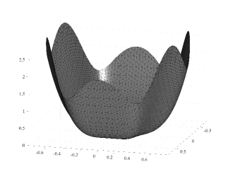
Figure 1: Elevation of the norm of velocity (cut elements are triangulated for graphics purpose only).

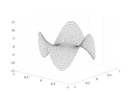
Figure 2: Elevation of the pressure.

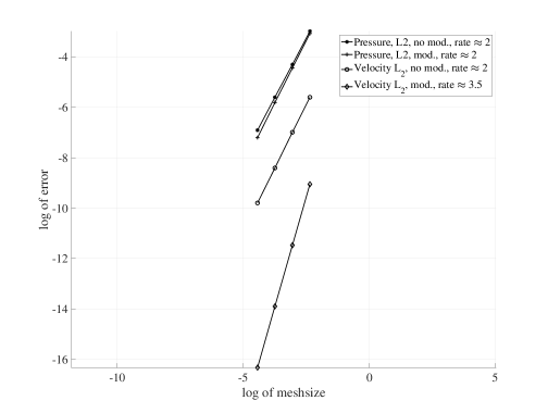
Figure 3: Convergence results.

References

• [1] R. Becker, E. Burman, and P. Hansbo. A Nitsche extended finite element method for incompressible elasticity with discontinuous modulus of elasticity. Comput. Methods Appl. Mech. Engrg., 198(41-44):3352–3360, 2009.
• [2] E. Burman. Ghost penalty. C. R. Math. Acad. Sci. Paris, 348(21-22):1217–1220, 2010.
• [3] E. Burman, S. Claus, P. Hansbo, M. G. Larson, and A. Massing. CutFEM: discretizing geometry and partial differential equations. Internat. J. Numer. Methods Engrg., 104(7):472–501, 2015.
• [4] E. Burman, S. Claus, and A. Massing. A stabilized cut finite element method for the three field Stokes problem. SIAM J. Sci. Comput., 37(4):A1705–A1726, 2015.
• [5] E. Burman and P. Hansbo. Fictitious domain methods using cut elements: III. A stabilized Nitsche method for Stokes’ problem. ESAIM Math. Model. Numer. Anal., 48(3):859–874, 2014.
• [6] E. Burman, P. Hansbo, and M. G. Larson. A cut finite element method with boundary value correction. Math. Comp., 87(310):633–657, 2018.
• [7] J. Guzmán and M. Olshanskii. Inf-sup stability of geometrically unfitted Stokes finite elements. Math. Comp., in press, http://dx.doi.org/10.1090/mcom/3288
• [8] P. Hansbo, M. G. Larson, and S. Zahedi. A cut finite element method for a Stokes interface problem. Appl. Numer. Math., 85:90–114, 2014.
• [9] P. Lederer, C.-M. Pfeiler, C. Wintersteiger, and C. Lehrenfeld. Higher order unfitted FEM for Stokes interface problems. Proc. Appl. Math. Mech., 16:7–10, 2016.
• [10] A. Massing, M. G. Larson, A. Logg, and M. E. Rognes. A stabilized Nitsche fictitious domain method for the Stokes problem. J. Sci. Comput., 61(3):604–628, 2014.
Refer to caption